The $\beta$-function for Yukawa theory at large $N_{f}$

Abstract

We compute the $\beta$-function for a massless Yukawa theory in a closed form at the order $\mathcal{O}(1/N_{f})$ in the spirit of the expansion in a large number of flavours $N_{f}$. We find an analytic expression with a finite radius of convergence, and the first singularity occurs at the coupling value $K=5$.

1 Introduction

The success of the Standard Model in describing the electroweak scale phenomena notwithstanding the apparent problems with the high-energy behaviour have lead to revival of interest in better understanding the UV properties of general gauge-Yukawa theories, see e.g. Refs Litim:2014uca ; Antipin:2017ebo ; Eichhorn:2016esv . In particular, gauge-Yukawa theories with a large number of fermion flavours, $N_{f}$, provide interesting candidates within the asymptotic-safety framework as opposed to the traditional asymptotic-freedom paradigm Gross:1973ju ; Politzer:1973fx .

The groundwork for these considerations was laid few decades ago with the computation of the leading large-$N_{f}$ behaviour of the gauge $\beta$-functions Espriu:1982pb ; PalanquesMestre:1983zy ; Gracey:1996he for $N_{f}$ fermion charged under the gauge group; see also Refs Holdom:2010qs ; Shrock:2013cca . The leading $1/N_{f}$ contribution to the $\beta$-function is obtained by resumming the gauge self-energy diagrams with ever increasing chain of fermion bubbles constituting a power series in $K=\alpha N_{f}/\pi$. It was noticed that this series has a finite radius of convergence; in the case of $\mathrm{U}(1)$ gauge group $K=15/2$. Furthermore, the leading $1/N_{f}$ contribution to the $\mathrm{U}(1)$ $\beta$-function has a negative pole at $K=15/2$, thereby suggesting that this behaviour could cure the Landau-pole behaviour of the SM $\mathrm{U}(1)$ coupling, see e.g. Refs Holdom:2010qs ; Mann:2017wzh ; Pelaggi:2017abg .

Recently, a further step towards a more complete understanding of these models was achieved by working out the leading $1/N_{f}$ contribution from the gauge sector to a Yukawa coupling Kowalska:2017pkt ; an extension to semi-simple gauge groups was discussed in Ref. Antipin:2018zdg . However, only a single fermion flavour was assumed to couple to the scalar, and the scalar self-energy remained uneffected by the $N_{f}$ fermion bubbles. Our work is the first step to bridge this remaining gap: we provide the leading $1/N_{f}$ $\beta$-function for pure Yukawa theory, where $N_{f}$ flavours of fermions couple to the scalar field via Yukawa interaction. We leave the more detailed study within a general gauge-Yukawa framework for future work. Interestingly, the pure Yukawa model is closely related to the Gross–Neveu–Yukawa model, whose critical exponents have been recently computed up to $1/N_{f}^{2}$ Gracey:2017fzu ; Manashov:2017rrx ; see also the earlier studies on the Gross–Neveu model e.g. Refs Gracey:1990wi ; Vasiliev:1992wr .

The paper is organized as follows: In Sec. 2 we introduce the framework and notations and in Sec. 3 give the expressions for the renormalization constants. In Sec. 4 we perform the resummations of the bubble chains and give closed form expressions for the renormalization constants. In Sec. 5 we collect the results, and write down the final expression for the $\beta$-function, and in Sec. 6 we conclude. Explicit formulas for the loop integrals are given in Appendix A.

2 The framework and definitions

We consider the massless Yukawa theory for a real scalar field, $\phi$, and a fermionic multiplet, $\psi$, consisting of $N_{f}$ flavours interacting through the usual Yukawa interaction:

$$\mathcal{L}_{\mathrm{Yuk}}=g\bar{\psi}\psi\phi.$$ (1)

We define the rescaled coupling,

$$K\equiv\frac{g^{2}}{4\pi^{2}}N_{f},$$ (2)

which is kept constant in the limit $N_{f}\to\infty$. The $\beta$-function of the rescaled coupling, $K$, can then be expanded in powers of $1/N_{f}$ as

$$\beta(K)\equiv\frac{\mathrm{d}K}{\mathrm{d}\ln\mu}=K^{2}\left[F_{0}+\frac{1}{N_{f}}F_{1}(K)\right]+\mathcal{O}\left(1/N_{f}^{2}\right).$$ (3)

The purpose of this paper is to compute $F_{0}$ and $F_{1}(K)$. The former is entirely fixed at the one-loop level and can be derived just by rescaling the well-known result for the $\beta$-function at that order, while the evaluation of $F_{1}(K)$ requires the resummation of diagrams in Fig. 1 involving all-order fermion-bubble chains.

$+$                                             $+$      

(a) Scalar self-energy corrections.

(b) Fermion self-energy correction.

(c) Vertex correction.

Figure 1: Scalar self-energy, fermion self-energy, and vertex corrections due to a chain of fermion bubbles.

The $\beta$-function can be obtained from

$$\beta=K^{2}\frac{\partial G_{1}(K)}{\partial K},$$ (4)

where $G_{1}$ is defined by

$$\text{ln}\,Z_{K}\equiv\text{ln}\,(Z_{S}^{-1}Z_{F}^{-2}Z_{V}^{2})=\sum_{n=1}^{\infty}\frac{G_{n}(K)}{\epsilon^{n}},$$ (5)

and $Z_{S}$, $Z_{F}$, and $Z_{V}$ are the renormalization constants for the scalar wave function, the fermion wave function, and the 1PI vertex, respectively. The scalar wave function renormalization constant is determined via

$$Z_{S}=1-\text{div}\{Z_{S}\Pi_{0}(p^{2},Z_{K}K,\epsilon)\},$$ (6)

where $\Pi_{0}(p^{2},K_{0},\epsilon)$ is the scalar self-energy divided by $p^{2}$, where $p$ is the external momentum. Here and in the following, $\text{div}{X}$ denotes the poles of $X$ in $\epsilon$. The self-energy can be written as

$$\Pi_{0}(p^{2},K_{0},\epsilon)=K_{0}\Pi^{(1)}(p^{2},\epsilon)+\frac{1}{N_{f}}\sum_{n=2}^{\infty}K_{0}^{n}\Pi^{(n)}(p^{2},\epsilon),$$ (7)

where $\Pi^{(1)}$ gives the one-loop result, and $\Pi^{(n)}$ the $n$-loop part containing $n-2$ fermion bubbles in the chain, and summing over the topologies given in Fig. 1(a). Other contributions are of higher order in $1/N_{f}$ and are thus omitted.

For the fermion self-energy and vertex renormalization constants, the lowest non-trivial contributions are already $\mathcal{O}(1/N_{f})$, and we, therefore, have

$$Z_{F}=1-\text{div}\left\{\Sigma_{0}(p^{2},Z_{K}K,\epsilon)\right\},$$ (8)

$$\Sigma_{0}(p^{2},K_{0},\epsilon)=\frac{1}{N_{f}}\sum_{n=1}^{\infty}K_{0}^{n}\Sigma^{(n)}(p^{2},\epsilon),$$ (9)

where $\Sigma^{(n)}$ is depicted in Fig. 1(b) with $n-1$ fermion bubbles. Similarly,

$$Z_{V}=1-\text{div}\left\{V_{0}(p^{2},Z_{K}K,\epsilon)\right\},$$ (10)

$$V_{0}(p^{2},K_{0},\epsilon)=\frac{1}{N_{f}}\sum_{n=1}^{\infty}K_{0}^{n}V^{(n)}(p^{2},\epsilon),$$ (11)

where $V^{(n)}$ again contains $n-1$ fermion bubbles and is shown diagrammatically in Fig 1(c).

Finally, we briefly comment on the scalar three-point and four-point functions, assuming that they are generated via fermion loops: the former exactly vanishes for massless fermions, while the latter is found to be already $\mathcal{O}(1/N_{f})$ at the lowest order. Therefore, they can be neglected for the purpose of our analysis.

3 Renormalization constants

In this section our goal is to extract the contributions to the renormalization constants that are $\mathcal{O}(1/N_{F})$ and relevant for the computation of the $\beta$-function.

Our starting point for $Z_{S}$ is Eq. (6). Using the expansion of the scalar self-energy, Eq. (7), we obtain

$$\begin{split}Z_{S}&=1-\text{div}\bigg{\{}Z_{S}Z_{K}K\Pi^{(1)}(p^{2},\epsilon)+\frac{1}{N_{f}}\sum_{n=2}^{\infty}Z_{S}(Z_{K}K)^{n}\Pi^{(n)}(p^{2},\epsilon)\bigg{\}}.\end{split}$$ (12)

Recalling that $Z_{K}\equiv Z_{S}^{-1}Z_{F}^{-2}Z_{V}^{2}$ and substituting Eqs (8) and (10), the first term between brackets can be written as

$$\text{div}\left\{Z_{S}Z_{K}\Pi^{(1)}(p^{2},\epsilon)K\right\}\\ =K\text{div}\left\{\Pi^{(1)}\right\}+\frac{1}{N_{f}}\text{div}\left\{2K\,\text{div}\left\{\Sigma_{0}(p^{2},Z_{K}K,\epsilon)-V_{0}(p^{2},Z_{K}K,\epsilon)\right\}\Pi^{(1)}(p^{2},\epsilon)\right\}.$$ (13)

The $\Pi^{(1)}$ part corresponds to the one-loop diagram and is given by

$$\begin{split}\Pi^{(1)}(p^{2},\epsilon)\equiv&\text{div}\left\{\Pi^{(1)}\right\}+\Pi^{(1)}_{\mathrm{F}}(p^{2},\epsilon)=\frac{1}{(4\pi)^{d/2-2}}\frac{G(1,1)}{2}(-p^{2})^{d/2-2}\\ =&\frac{1}{\epsilon}+\Pi^{(1)}_{\mathrm{F}}(p^{2},\epsilon),\end{split}$$ (14)

where $d=4-\epsilon$, the loop function, $G(1,1)$, is defined in Eq. (62) in Appendix A.1, and we have introduced the notation $\Pi^{(1)}_{\mathrm{F}}$ to indicate the finite part of $\Pi^{(1)}$. Then,

$$\begin{split}\text{div}&\left\{Z_{S}Z_{K}\Pi^{(1)}(p^{2},\epsilon)K\right\}\\ &=\frac{K}{\epsilon}+\frac{1}{N_{f}}\text{div}\bigg{\{}2K\,\text{div}\left\{\Sigma_{0}(p^{2},Z_{K}K,\epsilon)-V_{0}(p^{2},Z_{K}K,\epsilon)\right\}\\ &\qquad\qquad\qquad\quad\times\left(\text{div}\left\{\Pi^{(1)}\right\}+\Pi^{(1)}_{\mathrm{F}}(p^{2},\epsilon)\right)\bigg{\}}\\ &=\frac{K}{\epsilon}+\frac{1}{N_{f}}\text{div}\left\{2K\Pi^{(1)}_{\mathrm{F}}(p^{2},\epsilon)\left[\Sigma_{0}(p^{2},Z_{K}K,\epsilon)-V_{0}(p^{2},Z_{K}K,\epsilon)\right]\right\}\\ &\quad+\frac{1}{N_{f}}\times\ \text{higher poles},\end{split}$$ (15)

where the higher poles, i.e., higher than $1/\epsilon$, arise from the product of two divergent parts and will be omitted because they play no role in what follows. Then, at the lowest order in $1/N_{f}$,

$$Z_{S}=1-\frac{K}{\epsilon}+\mathcal{O}\left(1/N_{f}\right).$$ (16)

Therefore, every time $Z_{K}K$ appears in the argument of $\Sigma_{0}$ and $V_{0}$, it can be replaced by $K\left(1-\frac{K}{\epsilon}\right)^{-1}$; the additional contributions are higher order in $1/N_{f}$. For Eq. (15), we arrive at

$$\text{div}\left\{Z_{S}Z_{K}\Pi^{(1)}(p^{2},\epsilon)K\right\}\\ =\frac{K}{\epsilon}+\sum_{n=1}^{\infty}K^{n+1}\text{div}\left\{2\Pi^{(1)}_{\mathrm{F}}(p^{2},\epsilon)\left(1-\frac{K}{\epsilon}\right)^{-n}\left[\Sigma^{(n)}(p^{2},\epsilon)-V^{(n)}(p^{2},\epsilon)\right]\right\}.$$ (17)

Similarly, the second term of Eq. (12) reads

$$\frac{1}{N_{f}}\text{div}\left\{\sum_{n=2}^{\infty}Z_{S}(Z_{S}^{-1}K)^{n}\Pi^{(n)}(p^{2},\epsilon)\right\}=\frac{1}{N_{f}}\sum_{n=2}^{\infty}K^{n}\text{div}\left\{\left(1-\frac{K}{\epsilon}\right)^{1-n}\Pi^{(n)}(p^{2},\epsilon)\right\}.$$ (18)

Altogether, we can write $Z_{S}$ as

$$Z_{S}=1-\frac{K}{\epsilon}-\frac{1}{N_{f}}\sum_{n=2}^{\infty}K^{n}\left\{\left(1-\frac{K}{\epsilon}\right)^{1-n}\left(2\Pi^{(1)}_{\mathrm{F}}\left[\Sigma^{(n-1)}-V^{(n-1)}\right]+\Pi^{(n)}\right)\right\},$$ (19)

where the explicit functional dependence on $(p^{2},\epsilon)$ has been omitted to lighten the notation. Using the binomial expansion,

$$\left(1-\frac{K}{\epsilon}\right)^{1-n}=\sum_{i=0}^{\infty}\left(\begin{array}[]{c}n+i-2\\ i\end{array}\right)\frac{K^{i}}{\epsilon^{i}}$$ (20)

and performing a shift in the summation, $n\rightarrow n-i$, we find our final expression for $Z_{S}$:

$$Z_{S}=1-\frac{K}{\epsilon}-\frac{1}{N_{f}}\sum_{n=2}^{\infty}K^{n}\text{div}\left\{\sum_{i=0}^{n-2}\left(\begin{array}[]{c}n-2\\ i\end{array}\right)\frac{1}{\epsilon^{i}}\left(2\Pi^{(1)}_{\mathrm{F}}\left(\Sigma^{(n-i-1)}-V^{(n-i-1)}\right)+\Pi^{(n-i)}\right)\right\}.$$ (21)

We notice that Eq. (21) differs essentially from its counterpart in the QED PalanquesMestre:1983zy because of the contribution from the fermion self-energy and the vertex, which exactly cancel in QED because of the Ward identity.

The expression for $Z_{F}$ can be derived from Eq. (8) in a similar manner:

$$\begin{split}Z_{F}&=1-\frac{1}{N_{f}}\sum_{n=1}^{\infty}\text{div}\left\{\left(Z_{K}K\right)^{n}\Sigma^{(n)}(p^{2},\epsilon)\right\}\\ &=1-\frac{1}{N_{f}}\sum_{n=1}^{\infty}K^{n}\text{div}\left\{\left(1-\frac{K}{\epsilon}\right)^{-n}\Sigma^{(n)}(p^{2},\epsilon)\right\}\\ &=1-\frac{1}{N_{f}}\sum_{n=1}^{\infty}K^{n}\text{div}\left\{\sum_{i=0}^{n-1}\left(\begin{array}[]{c}n-1\\ i\end{array}\right)\frac{1}{\epsilon^{i}}\Sigma^{(n-i)}(p^{2},\epsilon)\right\},\end{split}$$ (22)

where we have again performed the same shift $n\rightarrow n-i$ in the last line. The derivation of $Z_{V}$ is completely analogous, and we can readily write the expression for $Z_{V}$:

$$Z_{V}=1-\frac{1}{N_{f}}\sum_{n=1}^{\infty}K^{n}\text{div}\left\{\sum_{i=0}^{n-1}\left(\begin{array}[]{c}n-1\\ i\end{array}\right)\frac{1}{\epsilon^{i}}V^{(n-i)}(p^{2},\epsilon)\right\}.$$ (23)

4 Resummation

In this section we provide closed formulas for Eqs (21), (22), and (23).

4.1 The vertex

By explicit computation, the $n$-loop contribution to $V_{0}$ is

$$\begin{split}V^{(n)}(p^{2},\epsilon)=&\frac{(-1)^{n}}{4}\left(\frac{1}{(4\pi)^{d/2-2}}\right)^{n}\left(\frac{G(1,1)}{2}\right)^{n-1}(-p^{2})^{n(d/2-2)}\\ &\times G\left(1,1-(n-1)(d/2-2)\right),\end{split}$$ (24)

where $G(n_{1},n_{2})$ is defined in Eq. (62). We notice that, as in Ref. PalanquesMestre:1983zy , Eq. (24) allows for the following expansion:

$$V^{(n)}(p^{2},\epsilon)=(-1)^{n}\frac{1}{n\epsilon^{n}}\frac{v(p^{2},\epsilon,n)}{2},$$ (25)

where

$$v(p^{2},\epsilon,n)=\sum_{j=0}^{\infty}v_{j}(p^{2},\epsilon)(n\epsilon)^{j},$$ (26)

and $v_{j}(p^{2},\epsilon)$ are regular in the limit $\epsilon\rightarrow 0$ for all $j$. In particular, $v_{0}(\epsilon)$ is independent of $p^{2}$ and is explicitly given by

$$v_{0}(\epsilon)=\frac{2\Gamma(2-\epsilon)}{\Gamma\left(1-\frac{\epsilon}{2}\right)^{2}\Gamma\left(2-\frac{\epsilon}{2}\right)\Gamma\left(\frac{\epsilon}{2}\right)\,\epsilon}.$$ (27)

Substituting Eqs (24) and (25) in Eq. (23), we find:

$$Z_{V}=1-\frac{1}{N_{f}}\sum_{n=1}^{\infty}(-K)^{n}\text{div}\left\{\sum_{j=0}^{n-1}\frac{1}{\epsilon^{n-j}}\sum_{i=0}^{n-1}\left(\begin{array}[]{c}n-1\\ i\end{array}\right)(-1)^{i}(n-i)^{j-1}\frac{v_{j}(p^{2},\epsilon)}{2}\right\}.$$ (28)

Then, by using the result of Ref. PalanquesMestre:1983zy ,

$$\sum_{i=0}^{n-1}\left(\begin{array}[]{c}n-1\\ i\end{array}\right)(-1)^{i}(n-i)^{j-1}=-\delta_{j,0}\frac{(-1)^{n}}{n},\ j=0,\dots,n-1,$$ (29)

Eq. (28) gets simplified to

$$Z_{V}=1+\frac{1}{2N_{f}}\sum_{n=1}^{\infty}\frac{K^{n}}{\epsilon^{n}}\frac{v_{0}(\epsilon)}{n}.$$ (30)

Expanding $v_{0}(\epsilon)$ as

$$v_{0}(\epsilon)=\sum_{j=0}^{\infty}v_{0}^{(j)}\epsilon^{j}$$ (31)

and keeping only the $1/\epsilon$ pole of Eq. (30), we find the closed formula for $Z_{V}$:

$$Z_{V}=1+\frac{1}{2\epsilon N_{f}}\sum_{n=1}^{\infty}\frac{K^{n}}{n}v_{0}^{(n-1)}=1+\frac{1}{2\epsilon N_{f}}\int_{0}^{K}v_{0}(t)\mathrm{d}t.$$ (32)

4.2 The fermion self-energy

The $n$-loop contribution to $\Sigma_{0}$ is found to be

$$\begin{split}\Sigma^{(n)}(p^{2},\epsilon)=&-\frac{(-1)^{n}}{8}\left(\frac{1}{(4\pi)^{d/2-2}}\right)^{n}\left(\frac{G(1,1)}{2}\right)^{n-1}(-p^{2})^{n(d/2-2)}\\ &\times\left[G(1,1-(n-1)(d/2-2))-G(1,-(n-1)(d/2-2))\right].\end{split}$$ (33)

Similarly to Eq. (24), Eq. (33) can be expanded as

$$\Sigma^{(n)}(p^{2},\epsilon)=-(-1)^{n}\frac{1}{n\epsilon^{n}}\frac{\sigma(p^{2},\epsilon,n)}{4},$$ (34)

where

$$\sigma(n,\epsilon,p^{2})=\sum_{j=0}^{\infty}\sigma_{j}(p^{2},\epsilon)(n\epsilon)^{j},$$ (35)

and $\sigma_{j}(p^{2},\epsilon)$ are regular for $\epsilon\rightarrow 0$. Again, $\sigma_{0}(\epsilon)$ is independent of $p^{2}$, and it is given by

$$\sigma_{0}(\epsilon)=-\frac{2^{5-\epsilon}\Gamma\left(\frac{3}{2}-\frac{\epsilon}{2}\right)}{\sqrt{\pi}(4-\epsilon)\Gamma\left(-\frac{\epsilon}{2}\right)\epsilon}\frac{\text{sin}\left(\frac{\pi\epsilon}{2}\right)}{\pi\epsilon}.$$ (36)

Using the same procedure as in the previous section, we find that only $\sigma_{0}(\epsilon)$ contributes to $Z_{F}$. Keeping only the $1/\epsilon$ pole, the closed formula for $Z_{F}$ is

$$Z_{F}=1-\frac{1}{4\epsilon N_{f}}\int_{0}^{K}\sigma_{0}(t)\mathrm{d}t.$$ (37)

4.3 The scalar self-energy

The evaluation of the bubble diagrams in Fig. 1(a) is quite cumbersome and is discussed in Appendix A.2. Here, we notice that the expression for $\Pi^{(n)}(p^{2},\epsilon)$, $n\geq 2$, allows for the following expansion:

$$\Pi^{(n)}=-\frac{3}{2}\frac{(-1)^{n}}{n(n-1)\epsilon^{n}}\pi(p^{2},\epsilon,n),$$ (38)

where

$$\pi(p^{2},\epsilon,n)=\sum_{j=0}^{\infty}\pi_{j}(p^{2},\epsilon)(n\epsilon)^{j},$$ (39)

and $\pi_{j}(p^{2},\epsilon)$ are regular for $\epsilon\rightarrow 0$. Similarly to the previous cases, $\pi_{0}(\epsilon)$ is independent of $p^{2}$.

In view of Eq. (21), we define

$$2\Pi^{(1)}_{\mathrm{F}}(p^{2},\epsilon)\left(\Sigma^{(n-1)}(p^{2},\epsilon)-V^{(n-1)}(p^{2},\epsilon)\right)+\Pi^{(n)}(p^{2},\epsilon)\equiv\frac{(-1)^{n}}{n(n-1)\epsilon^{n}}\xi(p^{2},\epsilon,n),$$ (40)

where

$$\xi(p^{2},\epsilon,n)\equiv n\epsilon\,\Pi^{(1)}_{\mathrm{F}}\left(\frac{\sigma(p^{2},\epsilon,n-1)}{2}+v(p^{2},\epsilon,n-1)\right)-\frac{3}{2}\pi(p^{2},\epsilon,n),$$ (41)

and

$$\xi(p^{2},\epsilon,n)=\sum_{j=0}^{\infty}\xi_{j}(p^{2},\epsilon)(n\epsilon)^{j},$$ (42)

with $\xi_{j}(\epsilon,p^{2})$ regular for $\epsilon\rightarrow 0$ for all $j$. In particular, $\xi_{0}(\epsilon)$ is independent of $p^{2}$ and is explicitly given by

$$\xi_{0}(\epsilon)=-\frac{(1-\epsilon)\Gamma(4-\epsilon)}{\Gamma\left(2-\frac{\epsilon}{2}\right)\Gamma\left(3-\frac{\epsilon}{2}\right)\pi\epsilon}\sin\left(\frac{\pi\epsilon}{2}\right)$$ (43)

Then, using the above definitions, Eq. (21) can be written as

$$\begin{split}Z_{S}&=1-\frac{K}{\epsilon}-\frac{1}{N_{f}}\sum_{n=2}^{\infty}K^{n}\text{div}\left\{\sum_{i=0}^{n-2}\left(\begin{array}[]{c}n-2\\ i\end{array}\right)\frac{1}{\epsilon^{i}}\frac{(-1)^{n-i}}{(n-i)(n-i-1)\epsilon^{n-i}}\xi(p^{2},\epsilon,n-i)\right\}\\ &=1-\frac{K}{\epsilon}-\frac{1}{N_{f}}\sum_{n=2}^{\infty}(-K)^{n}\text{div}\left\{\sum_{j=0}^{n-1}\frac{1}{\epsilon^{n-j}}\xi_{j}(p^{2},\epsilon)\sum_{i=0}^{n-2}\left(\begin{array}[]{c}n-2\\ i\end{array}\right)(-1)^{i}\frac{(n-i)^{j-1}}{(n-i-1)}\right\}.\end{split}$$ (44)

Moreover, we find that

$$\sum_{i=0}^{n-2}\left(\begin{array}[]{c}n-2\\ i\end{array}\right)(-1)^{i}\frac{(n-i)^{j-1}}{(n-i-1)}=\begin{cases}\frac{(-1)^{n}}{n}&j=0\\ \frac{(-1)^{n}}{n-1}&j=1,\dots,n-1\end{cases},$$ (45)

and therefore the expression for $Z_{S}$ can be significantly simplified:

$$\begin{split}Z_{S}&=1-\frac{K}{\epsilon}-\frac{1}{N_{f}}\sum_{n=2}^{\infty}K^{n}\,\text{div}\left\{\frac{1}{\epsilon^{n}}\left(\frac{\xi_{0}(\epsilon)}{n}+\frac{1}{n-1}\sum_{j=1}^{n-1}\xi_{j}(p^{2},\epsilon)\epsilon^{j}\right)\right\}\\ &=1-\frac{K}{\epsilon}-\frac{1}{N_{f}}\sum_{n=2}^{\infty}K^{n}\,\text{div}\left\{\frac{1}{\epsilon^{n}}\left(\frac{\xi_{0}(\epsilon)}{n}+\frac{1}{n-1}\sum_{j=1}^{\infty}\xi_{j}(p^{2},\epsilon)\epsilon^{j}\right)\right\}\\ &=1-\frac{K}{\epsilon}-\frac{1}{N_{f}}\sum_{n=2}^{\infty}K^{n}\,\text{div}\left\{\frac{1}{\epsilon^{n}}\left(\frac{\xi_{0}(\epsilon)}{n}+\frac{\xi(p^{2},\epsilon,1)-\xi_{0}(\epsilon)}{n-1}\right)\right\},\end{split}$$ (46)

where in the second line we extended the sum over $j$ up to $\infty$ without affecting the result, since all the terms for $j>n-1$ are finite. The function $\xi(p^{2},\epsilon,1)$, corresponding to

$$\xi(p^{2},\epsilon,1)\equiv\sum_{j=0}^{\infty}\xi_{j}(p^{2},\epsilon)\epsilon^{j},$$ (47)

can be evaluated by taking in Eq. (41) the limit $n\rightarrow 1$, although the latter is formally defined for $n\geq 2$. We find the following expression:

$$\xi(p^{2},\epsilon,1)=-\frac{\Gamma(4-\epsilon)}{\Gamma\left(2-\frac{\epsilon}{2}\right)\Gamma\left(3-\frac{\epsilon}{2}\right)\pi\epsilon}\sin\left(\frac{\pi\epsilon}{2}\right)\equiv\xi(\epsilon,1).$$ (48)

Few comments are in order: Eq. (48) ensures that $Z_{S}$ is independent of the external momentum $p^{2}$, as it should. This result comes from an exact cancellation among the different contributions of the scalar self-energy, the fermion self-energy, and the vertex in Eq. (41). In particular, we find that

$$\begin{split}\pi(p^{2},\epsilon,1)&=\frac{2}{3}\left(\frac{\sigma(p^{2},\epsilon,0)}{2}+v(p^{2},\epsilon,0)\right)\left[1+1\cdot\epsilon\,\Pi^{(1)}_{\mathrm{F}}(p^{2},\epsilon)\right]\\ &=\frac{2}{3}\left(\frac{\sigma_{0}(\epsilon)}{2}+v_{0}(\epsilon)\right)\left[1+\epsilon\,\Pi^{(1)}_{\mathrm{F}}(p^{2},\epsilon)\right],\end{split}$$ (49)

and therefore

$$\xi(\epsilon,1)=-\frac{\sigma_{0}(\epsilon)}{2}-v_{0}(\epsilon),$$ (50)

which is equivalent to Eq. (48). Interestingly, Eq. (49) only holds for $n=1$. All in all, the $p^{2}$ independence of Eq. (48) provides a non-trivial check for our computation. Moreover, we see that

$$\xi_{0}(\epsilon)=(1-\epsilon)\xi(\epsilon,1).$$ (51)

We are now ready to resum the series in Eq. (46). By expanding $\xi_{0}(\epsilon)$ as

$$\xi_{0}(\epsilon)=\sum_{j=0}^{\infty}\xi_{0}^{(j)}\epsilon^{j},$$ (52)

the $\frac{1}{n}$ term in Eq. (46) is given by

$$\begin{split}\sum_{n=2}^{\infty}\frac{K^{n}}{\epsilon^{n}}\frac{\xi_{0}(\epsilon)}{n}&=\frac{1}{\epsilon}\sum_{n=2}^{\infty}\frac{K^{n}}{\epsilon^{n}}\frac{\xi_{0}^{(n-1)}}{n}+\text{higher poles}\\ &=\frac{1}{\epsilon}\left(\,\sum_{n=0}^{\infty}K^{n+1}\frac{\xi_{0}^{(n)}}{n+1}-K\xi_{0}^{(0)}\right)+\text{higher poles}\\ &=\frac{1}{\epsilon}\int_{0}^{K}\left[\xi_{0}(t)-\xi_{0}(0)\right]\mathrm{d}t+\text{higher poles}.\end{split}$$ (53)

As for the $\frac{1}{n-1}$ term, using $\xi_{0}(\epsilon)=(1-\epsilon)\xi(\epsilon,1)$ and expanding $\xi(\epsilon,1)$ as

$$\xi(\epsilon,1)=\sum_{j=0}^{\infty}\tilde{\xi}^{(n)}\epsilon^{j},$$ (54)

we find

$$\begin{split}\sum_{n=2}^{\infty}\frac{K^{n}}{\epsilon^{n}}\frac{\epsilon\xi(\epsilon,1)}{n-1}&=\frac{K}{\epsilon}\sum_{n=0}^{\infty}\frac{K^{n+1}}{n+1}\tilde{\xi}^{(n)}+\text{higher poles}\\ &=\frac{K}{\epsilon}\int_{0}^{K}\xi(t,1)\mathrm{d}t+\text{higher poles}.\end{split}$$ (55)

Finally, the closed formula for $Z_{S}$ reads

$$Z_{S}=1-\frac{K}{\epsilon}-\frac{1}{\epsilon N_{f}}\int_{0}^{K}\left[\xi_{0}(t)-\xi_{0}(0)+\xi(t,1)K\right]\mathrm{d}t.$$ (56)

5 The $\beta$-function

Using the results of the previous section together with Eq. (5), we can finally proceed to evaluating the $\beta$-function. First, we find that

$$G_{1}(K)=K+\frac{1}{N_{f}}\int_{0}^{K}\left(\xi_{0}(t)-\xi_{0}(0)+\xi(t,1)K+\frac{\sigma_{0}(t)}{2}+v_{0}(t)\right)\mathrm{d}t.$$ (57)

Now, it is straightforward to compute the $\beta$-function:

$$\begin{split}\beta(K)=&K^{2}+\frac{K^{2}}{N_{f}}\left\{-\xi_{0}(0)+\xi(K,1)+\frac{\sigma_{0}(K)}{2}+v_{0}(K)+\int_{0}^{K}\xi(t,1)\mathrm{d}t\right\}.\end{split}$$ (58)

Recalling Eq. (50) and using $\xi_{0}(0)=-\frac{3}{2}$, Eq. (58) can be further simplified to

$$\frac{\beta(K)}{K^{2}}=1+\frac{1}{N_{f}}\left\{\frac{3}{2}+\int_{0}^{K}\xi(t,1)\mathrm{d}t\right\}.$$ (59)

Finally, by comparison with Eq. (3), we see that $F_{0}=1$ and

$$F_{1}(K)=\frac{3}{2}+\int_{0}^{K}\xi(t,1)\mathrm{d}t.$$ (60)

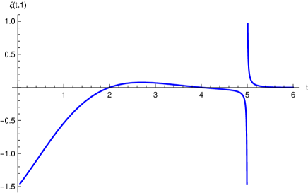
We plot the integrand, $\xi(t,1)$, in Fig. 2. We have checked that our $\beta$-function agrees at the leading order in $N_{f}$ up to four-loop level by comparing with the result of Ref. Zerf:2017zqi , and with the result extracted from the critical exponents in Gross–Neveu–Yukawa model computed using a different technique Gracey:2017fzu .

Finally, let us comment on the pole structure: the integrand, $\xi(t,1)$, has the first pole occuring at $t=5$, which results in a logarithmic singularity for $F_{1}(K)$ around $K=5$. Due to the sign of $\xi(t,1)$, we see that $F_{1}(K)$ approaches large negative values for $K\rightarrow 5^{-}$. This suggests the existence of a UV fixed point at $K_{\text{UV}}\lesssim 5$ such that $F_{1}(K_{\text{UV}})=-N_{f}$.

Figure 2: The function $\xi(t,1)$.

6 Conclusions

We have computed the leading $1/N_{f}$ contribution for the $\beta$-function in Yukawa theory with $N_{f}$ fermion flavours coupling to a real scalar. We obtained a closed form expression for the $\beta$-function up to order $\mathcal{O}(1/N_{f})$. This expression has a finite radius of convergence, and the first singularity occurs at $K=5$.

The present result adds an interesting ingredient to models with a large number of fermions, and makes a contribution to better understand the UV behaviour of gauge-Yukawa theories.

Appendix A Loop integrals

We here provide some explicit formulas. We follow closely the notations of Ref. Grozin:2003ak .

A.1 The vertex and the fermion self-energy

As shown in Eqs (24) and (33), the 1PI vertex and the fermion self-energy involve only the function $G(n_{1},n_{2})$, independently of the number of bubbles. This corresponds to the one-loop integral

$$\int\frac{d^{d}k}{(2\pi)^{d}}\frac{1}{D_{1}^{n_{1}}D_{2}^{n_{2}}}=\mathrm{i}\frac{1}{(4\pi)^{d/2}}(-p^{2})^{d/2-n_{1}-n_{2}}(-1)^{n_{1}+n_{2}}G(n_{1},n_{2}),$$ (61)

where $D_{1}=(k+p)^{2}$ and $D_{2}=k^{2}$. Explicitly,

$$G(n_{1},n_{2})=\frac{\Gamma(-d/2+n_{1}+n_{2})\Gamma(d/2-n_{1})\Gamma(d/2-n_{2})}{\Gamma(n_{1})\Gamma(n_{2})\Gamma(d-n_{1}-n_{2})}.$$ (62)

A.2 The scalar self-energy

Unlike the 1PI vertex and the fermion self-energy, the $n$-loop contribution to the scalar self-energy, $\Pi_{0}$, indicated by $\Pi^{(n)}$, cannot be written in terms of $G(n_{1},n_{2})$ functions only. In fact, $\Pi^{(n)}$ is given by ($n\geq 2$):

$$\begin{split}p^{2}\Pi^{(n)}(p^{2},\epsilon)=&-(4\pi^{2})^{2}(-1)^{n}\left(\frac{1}{(4\pi)^{d/2-2}}\frac{G(1,1)}{2}\right)^{n-2}(-1)^{\alpha}\int\frac{d^{d}k_{1}}{(2\pi)^{d}}\int\frac{d^{d}k_{2}}{(2\pi)^{d}}\\ &\bigg{\{}\frac{6}{(p+k_{1})^{2}k_{2}^{2}((k_{1}-k_{2})^{2})^{1-\alpha}}-\frac{2}{k_{1}^{2}(p+k_{1})^{2}k_{2}^{2}((k_{1}-k_{2})^{2})^{-\alpha}}\\ &-\frac{2p^{2}}{k_{1}^{2}(p+k_{1})^{2}k_{2}^{2}((k_{1}-k_{2})^{2})^{1-\alpha}}+\frac{2p^{2}}{k_{1}^{4}(p+k_{1})^{2}k_{2}^{2}((k_{1}-k_{2})^{2})^{-\alpha}}\\ &-\frac{2p^{2}}{k_{1}^{2}(k_{1}+p)^{2}(k_{2}+p)^{2}k_{2}^{2}((k_{1}-k_{2})^{2})^{-\alpha}}\bigg{\}},\end{split}$$ (63)

where $\alpha=(n-2)(d/2-2)=-(n-2)\epsilon/2$. Eq. (63) requires two-loop integrals which can be performed according to the formula in Ref. Grozin:2003ak :

$$\int\frac{d^{d}k_{1}}{(2\pi)^{d}}\int\frac{d^{d}k_{2}}{(2\pi)^{d}}\frac{1}{D_{1}^{n_{1}}D_{2}^{n_{2}}D_{3}^{n_{3}}D_{4}^{n_{4}}D_{5}^{n_{5}}}=(-1)^{1+\sum n_{i}}\frac{\pi^{d}(-p^{2})^{d-\sum n_{i}}}{(2\pi)^{2d}}G(n_{1},n_{2},n_{3},n_{4},n_{5}),$$ (64)

where $D_{1}=(k_{1}+p)^{2}$, $D_{2}=(k_{2}+p)^{2}$, $D_{3}=k_{1}^{2}$, $D_{4}=k_{2}^{2}$, $D_{5}=(k_{1}-k_{2})^{2}$. The functions $G(n_{1},n_{2},n_{3},n_{4},n_{5})$ are symmetric with respect to the following index exchanges: $(1\leftrightarrow 2,3\leftrightarrow 4)$ and $(1\leftrightarrow 3,2\leftrightarrow 4)$. Moreover, they reduce to a product of $G(n_{1},n_{2})$ if at least one of the entries is zero:

$$G(n_{1},n_{2},n_{3},n_{4},0)=G(n_{1},n_{3})G(n_{2},n_{4}),$$ (65)

$$G(0,n_{2},n_{3},n_{4},n_{5})=G(n_{3},n_{5})G(n_{2},n_{3}+n_{4}+n_{5}-d/2).$$ (66)

It turns out that the first four integrals in Eq. (63) can always be written in terms of $G(n_{1},n_{2})$ making use of Eqs (65) and (66).

However, the last integral in Eq. (63) involves $G(1,1,1,1,(n-2)\epsilon/2)$ and, for $n>2$, its expression can be obtained in terms of hypergeometric functions $\vphantom{F}{}_{3}F_{2}$ by means of the Gegenbauer technique Kotikov:1995cw . We have evaluated the function $G(1,1,1,1,(n-2)\epsilon/2)$ recursively according to Eqs (2.19) and (2.21) in Ref. Grozin:2003ak .

References

- (1) D. F. Litim and F. Sannino, Asymptotic safety guaranteed, JHEP 12 (2014) 178, [arXiv:1406.2337].
- (2) O. Antipin and F. Sannino, Conformal Window 2.0: The large safe story, Phys. Rev. D97 (2018), no. 11 116007, [arXiv:1709.02354].
- (3) A. Eichhorn, A. Held, and J. M. Pawlowski, Quantum-gravity effects on a Higgs-Yukawa model, Phys. Rev. D94 (2016), no. 10 104027, [arXiv:1604.02041].
- (4) D. J. Gross and F. Wilczek, Asymptotically Free Gauge Theories - I, Phys. Rev. D8 (1973) 3633–3652.
- (5) H. D. Politzer, Reliable Perturbative Results for Strong Interactions?, Phys. Rev. Lett. 30 (1973) 1346–1349. [,274(1973)].
- (6) D. Espriu, A. Palanques-Mestre, P. Pascual, and R. Tarrach, The Function in the 1/ Expansion, Z. Phys. C13 (1982) 153.
- (7) A. Palanques-Mestre and P. Pascual, The 1/ Expansion of the and Beta Functions in QED, Commun. Math. Phys. 95 (1984) 277.
- (8) J. A. Gracey, The QCD -function at O(1/), Phys. Lett. B373 (1996) 178–184, [hep-ph/9602214].
- (9) B. Holdom, Large N flavor beta-functions: a recap, Phys. Lett. B694 (2011) 74–79, [arXiv:1006.2119].
- (10) R. Shrock, Study of Possible Ultraviolet Zero of the Beta Function in Gauge Theories with Many Fermions, Phys. Rev. D89 (2014), no. 4 045019, [arXiv:1311.5268].
- (11) R. Mann, J. Meffe, F. Sannino, T. Steele, Z.-W. Wang, and C. Zhang, Asymptotically Safe Standard Model via Vectorlike Fermions, Phys. Rev. Lett. 119 (2017), no. 26 261802, [arXiv:1707.02942].
- (12) G. M. Pelaggi, A. D. Plascencia, A. Salvio, F. Sannino, J. Smirnov, and A. Strumia, Asymptotically Safe Standard Model Extensions?, Phys. Rev. D97 (2018), no. 9 095013, [arXiv:1708.00437].
- (13) K. Kowalska and E. M. Sessolo, Gauge contribution to the 1/NF expansion of the Yukawa coupling beta function, JHEP 04 (2018) 027, [arXiv:1712.06859].
- (14) O. Antipin, N. A. Dondi, F. Sannino, A. E. Thomsen, and Z.-W. Wang, Gauge-Yukawa theories: Beta functions at large , arXiv:1803.09770.
- (15) J. A. Gracey, Critical exponent in the Gross-Neveu-Yukawa model at , Phys. Rev. D96 (2017), no. 6 065015, [arXiv:1707.05275].
- (16) A. N. Manashov and M. Strohmaier, Correction exponents in the Gross–Neveu–Yukawa model at , Eur. Phys. J. C78 (2018), no. 6 454, [arXiv:1711.02493].
- (17) J. A. Gracey, Calculation of exponent eta to O(1/N**2) in the O(N) Gross-Neveu model, Int. J. Mod. Phys. A6 (1991) 395–408. [Erratum: Int. J. Mod. Phys.A6,2755(1991)].
- (18) A. N. Vasiliev, S. E. Derkachov, N. A. Kivel, and A. S. Stepanenko, The 1/n expansion in the Gross-Neveu model: Conformal bootstrap calculation of the index eta in order 1/n**3, Theor. Math. Phys. 94 (1993) 127–136. [Teor. Mat. Fiz.94,179(1993)].
- (19) N. Zerf, L. N. Mihaila, P. Marquard, I. F. Herbut, and M. M. Scherer, Four-loop critical exponents for the Gross-Neveu-Yukawa models, Phys. Rev. D96 (2017), no. 9 096010, [arXiv:1709.05057].
- (20) A. G. Grozin, Lectures on multiloop calculations, Int. J. Mod. Phys. A19 (2004) 473–520, [hep-ph/0307297].
- (21) A. V. Kotikov, The Gegenbauer polynomial technique: The Evaluation of a class of Feynman diagrams, Phys. Lett. B375 (1996) 240–248, [hep-ph/9512270].