Quantifying discretization errors for soft-tissue simulation in computer assisted surgery: a preliminary study

Abstract

Errors in biomechanics simulations arise from modeling and discretization. Modeling errors are due to the choice of the mathematical model whilst discretization errors measure the impact of the choice of the numerical method on the accuracy of the approximated solution to this specific mathematical model. A major source of discretization errors is mesh generation from medical images, that remains one of the major bottlenecks in the development of reliable, accurate, automatic and efficient personalized, clinically-relevant Finite Element (FE) models in biomechanics. The impact of mesh quality and density on the accuracy of the FE solution can be quantified with a posteriori error estimates. Yet, to our knowledge, the relevance of such error estimates for practical biomechanics problems has seldom been addressed, see [25]. In this contribution, we propose an implementation of some a posteriori error estimates to quantify the discretization errors and to optimize the mesh. More precisely, we focus on error estimation for a user-defined quantity of interest with the Dual Weighted Residual (DWR) technique. We test its applicability and relevance in two situations, corresponding to computations for a tongue and an artery, using a simplified setting, i.e., plane linearized elasticity with contractility of the soft-tissue modeled as a pre-stress. Our results demonstrate the feasibility of such methodology to estimate the actual solution errors and to reduce them economically through mesh refinement.

1 Introduction

Patient-specific finite element models of soft tissue and organs have received an increasing amount of interest in the last decades. Such finite element models are widely employed to investigate both, the underlying mechanisms that drive normal physiology of biological soft tissues [8, 44, 54], and the mechanical factors that contribute to the onset and development of diseases such as pressure ulcers [77, 117], atherosclerosis or aneurysms [70, 9, 111], or multilevel lumbar degenerative disc diseases [97, 113], to name a few. Finite element models are also valuable tools that contribute to the development of medical devices, see e.g. vascular stent-grafts [100], artificial facet systems for spinal fusion [51] or knee braces [101]. They have the potential to improve prevention strategies [79, 124], surgical planning [21] and pedagogical simulators for medical training [20, 32, 28, 33] .

In this context, one major issue is meshing, since the reliability of the predicted mechanical response arising from computer simulation heavily relies on the quality of the underlying finite element mesh: if some elements of the mesh are too distorted or if the mesh is too coarse in some regions, the numerical solution may deteriorate significantly [55].

Whilst generating meshes of complex shapes with tetrahedral elements is generally possible thanks to advanced meshing algorithms, e.g. [49, 108], low-order Lagrange tetrahedral elements are unsuitable for most biomechanical problems due to volumetric locking. To circumvent such issues, strain smoothing approaches were developed [94, 71], which have the drawback of leading to larger system matrix bandwidth, but the advantage of being easily parallelized on graphical processing units thanks to nodal integration. Hexahedral low-order Lagrange elements alleviate locking issues, but research on the automatic generation of hexahedral meshes is still ongoing [18, 99, 107], spurred by a recrudescent surge in research on polyhedral mesh generation [60, 83, 24, 31, 128] and approximations such as the virtual finite element method [16], hybrid high-order (HHO) methods [38], polyhedral finite elements [119, 67, 86, 43], smoothed finite elements [114], scaled finite elements [119, 87], for various applications, including large strain hyper-elasticity [104, 1] and optimization [30, 30, 89].

The patient-specific mesh has to be built from segmented medical images (CT, MRI, ultra-sound), and has to conform to anatomical details with potentially complex topologies and geometries [123, 17, 6], which led to the design of algorithms that aim to optimize the quality of the generated mesh by reducing the distortion of the elements [131, 69, 115]. These algorithms may also have to satisfy a number of additional constraints such as minimizing human intervention (automation), preservation of certain important anatomical details or robustness with respect to data [34, 7, 61, 116, 76]. In general the quality of a given mesh can be assessed through purely geometrical criteria, that allow in some way to quantify the distortion of the geometry of the elements and how far they are from their ideal shape [45, 22, 26, 47].

To circumvent or simplify the mesh generation issue, implicit/immersed boundary approaches have been proposed, where the mesh does not conform to the geometry, which is treated by implicit functions such as level sets and enriched finite element methods. This idea was proposed in [81] and later generalized in [84, 85], [58, 27], [75, 66] and [109, 126, 46], in combination with (goal-oriented) error estimates. Although promising, applications of such approaches to patient-specific geometries remain in their infancy, see a review of related methods in [19]. Yet another approach consists in directly using the image as a model which could enable simulations without any mesh generation [72]. In “image as a model”, the boundary of the domain is smeared, which significantly complicates imposition of boundary conditions, particularly contact. Finally, meshless methods [88] are possible alternatives which may simplify biomechanics simulations by relaxing the constraints posed on mesh quality and simplifying local mesh adaptation. Comparatively to Galerkin meshfree methods [73, 37, 74], point collocation methods [11], also known as generalized finite difference methods, are potentially competitive as they do not require any numerical integration. Quality control of such collocation methods remains an open problem, as well as conditioning of the system matrix, which is strongly related to the choice of the stencil [36]. On the other hand, collocation methods are easily parallelized, for instance on graphical processing units.

Beyond mesh quality, mesh density is another, related, parameter which must be controlled during biomechanics simulations. Solutions must be obtained on commodity hardware within clinical time scales: milliseconds (for surgical training); minutes (for surgical assistance); hours (for surgical planning). Therefore, and although this would lead to the most accurate solution, it is impractical to use a uniformly fine mesh over the whole domain. This remark begs the question: “given a tolerable error level, what is the coarsest possible mesh which will provide the required accuracy.” This leads to the notion of “mesh optimality,” which is achieved for an optimal balance between the accuracy in a given quantity of interest to the user and the associated computational cost. It is probably intuitively understood that this “optimality” criterion, and the resulting optimized mesh both depend on the quantity of interest and that, in general, the optimal mesh will be non-uniform, displaying local refinement around specific regions. A possible criterion for mesh adaptation can be any a priori knowledge of the problem or its solution such as geometry, material properties or boundary layers e.g. localized loads, contacts, sharp features, material interfaces. Similarly, knowledge of the quantity of interest can help guide local mesh refinement. Nevertheless, such mesh refinement guidelines are generally ad hoc and cannot guarantee the resulting mesh will be optimal.

To summarize, the, standard, piecewise linear or quadratic Lagrange-based, finite element method is still the most popular technology to solve biomechanics problems. The choice of an optimal mesh, in particular its local refinement level for given problems and quantities of interest remains an open issue. Moreover, without knowing the finite element solution itself, it is practically impossible to quantify the adequacy of a given mesh only from heuristics or other ad hoc criteria derived from a priori knowledge of the problem or its exact solution.

As a result, we aim at addressing the following two questions in this paper:

1. For a patient-specific finite element computation, can we provide some information to the user about the accuracy of the numerical solution, namely can we compute an approximate discretization error caused by the choice of the mesh? By discretization error, we mean the difference between the finite element solution and the exact solution of the same boundary value problem on the same geometry.

2. Can the numerical solution be used to optimize the mesh in the critical regions only, to achieve maximum accuracy for a given computational cost, or, conversely, to achieve a given accuracy with a minimum computational cost?

For the sake of simplicity we do not consider

1. modeling errors, which arise due to the approximation of the geometry, physical assumptions, and uncertainty on material parameters,

2. numerical errors, which arise due to linearization, iterative solvers, and machine precision.

In this paper, we investigate the capability of a posteriori error estimates [3, 127] to provide useful information about the discretization error. A posteriori error estimates are quantities computed from the numerical solution, that indicate the magnitude of the local error. These estimates are at the core of mesh adaptive techniques [92]. Many a posteriori error estimation methods have been developed in the numerical analysis community. These methods have different theoretical and practical properties. However, despite their great potential, error estimates, to the best of our knowledge, have rarely been considered for patient-specific finite element simulations in the biomechanical community. The only reference known to us which addresses discretization error estimation in biomechanics is the very recent paper [25] who consider simple but real-time error estimation approaches for needle insertion.

We limit our study to a simplified setting in order to gain preliminary insights into the behaviour of such a posteriori error estimates and to address with the first technical difficulties. We focus on two-dimensional linear elasticity (plane strain) problems, with simple boundary conditions (prescribed displacements and tractions), and we assume triangular meshes. This is somehow restrictive in comparison to current practice in soft-tissue simulation. Among the existing a posteriori error estimates, we focus on Dual Weighted Residuals (DWR), as presented in, e.g., [13, 14] (see also [96, 95, 102, 80, 50, 10]). Indeed this method allows to estimate the error for a given quantity of interest. As a matter of fact, for the majority of applications, controlling the error in the energy norm is not relevant, and the error must be controlled for a specific quantity of interest to the user (e.g., stress intensity factors, shear stress or strain intensity at specific locations). The DWR method is conveniently implemented in the standard finite element library FEniCS [78] and we make use of the implementation described in detail in the paper of Rognes and Logg [110], with minor modifications.

This paper is organized as follows. In Section 2, we present the linear elastic problem, the corresponding finite element method, the a posteriori error estimates as well as the algorithm for mesh refinement. In Section 3, we consider two simplified test-cases, inspired by patient-specific biomechanics, where the current methodology is applied. The results are discussed in Section 4.

2 Material and methods

We first present the general problem considered in this contribution, that represents a simplified setting for contractile soft-tissue simulation. We then describe in details the computation of the a posteriori error estimate: a global estimator that provides an estimation of the discretization error and a local estimator that drives the mesh refinement. We end this section with the description of a simple algorithm for mesh refinement.

We first introduce some useful notations. In what follows, bold letters such as ${\bf u},{\bf v}$, indicate vector or tensor valued quantities, while the capital ones (e.g., ${\bf V}$, ${\bf K}$) represent functional sets involving vector fields. As usual, we denote by $(H^{s}(\cdot))^{d}$, $s\in\mathbb{R}$, $d=1,2,3$, the Sobolev spaces in one, two or three space dimensions [2]. In the sequel the symbol $|\cdot|$ will either denote the Euclidean norm in $\mathbb{R}^{d}$, or the measure of a domain in $\mathbb{R}^{d}$.

2.1 Setting: a “toy” boundary value problem in linear elasticity

We consider an elastic body whose reference configuration is represented by the domain $\Omega$ in $\mathbb{R}^{2}$. We consider the plane strain formulation, and allow only small deformations. We suppose that $\partial\Omega$ consists of two disjoint parts $\Gamma_{D}$ and $\Gamma_{N}$, with meas$(\Gamma_{D})>0$. The unit outward normal vector on $\partial\Omega$ is denoted by ${\bf n}$. A displacement ${\bf u}_{D}={\bf 0}$ is applied on $\Gamma_{D}$, and the body is subjected to volume forces ${\bf f}\in(L^{2}(\Omega))^{2}$ and surface loads ${\bf F}\in(L^{2}(\Gamma_{N}))^{2}$. We introduce the bilinear form

$$a({\bf v},{\bf w}):=\int_{\Omega}\mbox{\boldmath{$\sigma$}}({\bf v}):\mbox{\boldmath{$\varepsilon$}}({\bf w})\leavevmode\nobreak\ d{\bf x},$$

which represents the (internal) virtual work associated to passive elastic properties. The notation $\mbox{\boldmath{$\varepsilon$}}({\bf v})=\frac{1}{2}(\mbox{\boldmath{$\nabla$}}{\bf v}+\mbox{\boldmath{$\nabla$}}{\bf v}^{{}^{T}})/2$ represents the linearized strain tensor field, and $\mbox{\boldmath{$\sigma$}}=(\sigma_{ij})$, $1\leq i,j\leq 2$, stands for the stress tensor field, assumed to be given by Hooke’s law. The linear form

$$l_{E}({\bf w}):=\int_{\Omega}{\bf f}\cdot{\bf w}\leavevmode\nobreak\ d{\bf x}+\int_{\Gamma_{N}}{\bf F}\cdot{\bf w}\leavevmode\nobreak\ ds$$

stands for the virtual work of external loads in the body and on its surface. Finally we represent in a very simplified manner the active properties of soft-tissue as a linear anisotropic pre-stress

$$l_{A}({\bf w}):=-\beta T\int_{\omega_{A}}\left(\mbox{\boldmath{$\varepsilon$}}({\bf w}){\bf e}_{A}\right)\cdot{\bf e}_{A}\leavevmode\nobreak\ d{\bf x},$$

where $\omega_{A}$ is the part of the body where muscle fibers are supposed to act, $T\geq 0$ is a scalar which stands for the tension of the fibers, ${\bf e}_{A}$ is a field of unitary vectors that stands for muscle fibers orientation, and $\beta\in[0,1]$ is the activation parameter. When $\beta=0$ there is no activation of the muscle fibers, and the value $\beta=1$ corresponds to the maximum activation. This modeling can be viewed as a linearization of some more sophisticated active stress models of contractile tissues (see, e.g., [35, 98]).

We want to solve the following weak problem

$$\left\{\begin{array}[]{l}\textrm{Find a displacement }{\bf u}\in{\bf V}\textrm{ such that}\\ \vskip 3.0pt plus 1.0pt minus 1.0pt\cr a({\bf u},{\bf v})=l({\bf v}),\quad\forall\,{\bf v}\in{\bf V},\end{array}\right.$$ (1)

where $l(\cdot)=l_{E}(\cdot)+l_{A}(\cdot)$, and where ${\bf u}$ and ${\bf v}$ lie in the space of admissible displacements

$${\bf V}:=\big{\{}{\bf v}\in H^{1}(\Omega)^{2}\,|\,\leavevmode\nobreak\ {\bf v}={\bf 0}\text{\leavevmode\nobreak\ on\leavevmode\nobreak\ }\Gamma_{D}\big{\}}.$$

From the displacement field, we are interested in computing a linear quantity

$$J:{\bf V}\ni{\bf u}\mapsto J({\bf u})\in\mathbb{R},$$ (2)

which can be defined according to a specific application and the interest of each practitioner. Thereby, the quantity $J$ will be aptly called quantity of interest (QoI). We will provide its expression(s) for each test case.

2.2 Finite element method

Consider a family of meshes $({\cal K}_{h})_{h>0}$ constituted of triangles and assumed to be subordinated to the decomposition of the boundary $\partial\Omega$ into $\Gamma_{D}$ and $\Gamma_{N}$. For a mesh ${\cal K}_{h}$, we denote by ${\cal E}_{h}$ the set of edges, by ${\cal E}^{int}_{h}:=\{E\in{\cal E}_{h}:E\subset\Omega\}$ the set of interior edges, and by ${\cal E}^{N}_{h}:=\{E\in{\cal E}_{h}:E\subset\Gamma_{N}\}$ the set of boundary edges that correspond to Neumann conditions (we assume that any boundary edge is either inside $\Gamma_{N}$ or inside $\Gamma_{D}$). For an element $K$ of $\mathcal{K}_{h}$, we set ${\cal E}_{K}$ the set of edges of $K$, ${\cal E}_{K}^{int}:={\cal E}_{K}\cap{\cal E}_{h}^{int}$ and ${\cal E}_{K}^{N}:={\cal E}_{K}\cap{\cal E}_{h}^{N}$. We also assume that each element $K$ is either completely inside $\omega_{A}$ or completely outside it. Let $\sigma$ be a second-order tensorial field in $\Omega$, which is assumed to be piecewise continuous. We define the jump of $\sigma$ across an interior edge $E$ of an element $K$, at a point ${\bf y}\in E$, as follows

$$[[\sigma]]_{E,K}({\bf y}):=\lim\limits_{\alpha\rightarrow 0^{+}}\left(\mbox{\boldmath{$\sigma$}}({\bf y}+\alpha{\bf n}_{E,K})-\mbox{\boldmath{$\sigma$}}({\bf y}-\alpha{\bf n}_{E,K})\right){\bf n}_{E,K},$$

where ${\bf n}_{E,K}$ is the unit normal vector to $E$, pointing out of $K$.

The finite element space ${\bf V}_{h}\subset{\bf V}$ is built upon continuous Lagrange finite elements of degree $k=1,2$ (see, e.g., [42]), i.e.

$${\bf V}_{h}:=\left\{{\bf v}_{h}\in(\mathcal{C}^{0}(\overline{\Omega}))^{d}:{\bf v}_{h|K}\in(\mathbb{P}_{k}(K))^{d},\forall K\in\mathcal{K}_{h},{\bf v}_{h}={\bf 0}\mbox{ on }\Gamma_{D}\right\}.$$

Problem (1) is approximated by

$$\left\{\begin{array}[]{l}\textrm{Find }{\bf u}_{h}\in{\bf V}_{h}\mbox{ such that }\\ \vskip 3.0pt plus 1.0pt minus 1.0pt\cr a({\bf u}_{h},{\bf v}_{h})=l({\bf v}_{h}),\qquad\forall{\bf v}_{h}\in{\bf V}_{h}.\end{array}\right.$$ (3)

2.3 Goal-oriented error estimates

We compute goal-oriented error estimates using the Dual Weighted Residual (DWR) technique [13, 14] (see also [10, 50, 80, 95, 96, 102]), which is inspired from duality arguments (see, e.g., [41]). We follow the framework described in [110], with some minor changes and adaptations.

Let us consider ${\bf u}_{h}$ the solution to Problem (3). The weak residual is defined for all ${\bf v}\in{\bf V}$ by

$$r({\bf v}):=l({\bf v})-a({\bf u}_{h},{\bf v}).$$

Let ${\bf z}$ denote the solution to the dual problem:

$$\left\{\begin{array}[]{l}\mbox{Find }{\bf z}\in{\bf V}\mbox{ such that}\\ \vskip 3.0pt plus 1.0pt minus 1.0pt\cr a({\bf v},{\bf z})=J({\bf v}),\qquad\forall\,{\bf v}\in{\bf V}.\end{array}\right.$$ (4)

The DWR method, in a linear setting, relies on the fundamental observation that

$$J({\bf u})-J({\bf u}_{h})=a({\bf u},{\bf z})-a({\bf u}_{h},{\bf z})=l({\bf z})-a({\bf u}_{h},{\bf z})=r({\bf z}).$$ (5)

From this, we design an error estimator of $J({\bf u})-J({\bf u}_{h})$ as an approximation of the residual $r({\bf z})$. We detail the different steps below.

2.3.1 Numerical approximation of the dual problem and global estimator

The exact solution ${\bf z}$ to the dual system (4) is unknown in most of the practical situations, and thus needs to be approximated. Let us consider a finite element space $\widehat{{\bf V}}_{h}\subset{\bf V}$. This space is assumed to be finer than ${\bf V}_{h}$, for instance, made of continuous piecewise polynomials of order $k+1$. The approximation $\widehat{{\bf z}}_{h}$ of the solution to the dual problem ${\bf z}$ is obtained by solving the following approximate dual problem

$$\left\{\begin{array}[]{l}\mbox{Find }\widehat{\mathbf{z}}_{h}\in\widehat{{\bf V}}_{h}\mbox{ such that}\\ \vskip 3.0pt plus 1.0pt minus 1.0pt\cr a(\widehat{{\bf v}}_{h},\widehat{\mathbf{z}}_{h})=J(\widehat{{\bf v}}_{h}),\qquad\forall\,\widehat{{\bf v}}_{h}\in\widehat{{\bf V}}_{h}.\end{array}\right.$$ (6)

We define

$$\eta_{h}:=|r(\widehat{\mathbf{z}}_{h})|$$ (7)

as the global estimator that approximates the residual $r({\bf z})$.

2.3.2 Derivation of local estimators

Following [14, 110], we provide a local estimator of the error $|J({\bf u})-J({\bf u}_{h})|$, that can be written in a general form

$$\sum\limits_{K\in{\cal K}_{h}}\eta_{K},\quad\eta_{K}:=\left|\displaystyle\int_{K}R_{K}\cdot(\widehat{\mathbf{z}}_{h}-i_{h}\widehat{\mathbf{z}}_{h})d{\bf x}\,+\sum_{E\in{\cal E}_{K}}\int_{E}R_{E,K}\cdot(\widehat{\mathbf{z}}_{h}^{i}-i_{h}\widehat{\mathbf{z}}_{h})ds\,\right|,\quad\forall K\in{\cal K}_{h},$$ (8)

where the notation $i_{h}$ stands for the Lagrange interpolant onto ${\bf V}_{h}$.

The local element-wise and edge-wise residuals are given explicitly by

$$R_{K}:={\bf f}_{K}+{\bf div}\,\mbox{\boldmath{$\sigma$}}_{A}({\bf u}_{h})$$

and

$$R_{E,K}:=\begin{cases}-\dfrac{1}{2}[[\mbox{\boldmath{$\sigma$}}_{A}({\bf u}_{h})]]_{E,K}&\text{if}\leavevmode\nobreak\ E\in{\cal E}^{int}_{K},\\ {\bf F}_{E}-\mbox{\boldmath{$\sigma$}}_{A}({\bf u}_{h}){\bf n}_{E,K}&\text{if}\leavevmode\nobreak\ E\in{\cal E}^{N}_{K},\end{cases}$$

where

$$\mbox{\boldmath{$\sigma$}}_{A}:=\mbox{\boldmath{$\sigma$}}({\bf u}^{h})+\beta T({\bf e}_{A}\otimes{\bf e}_{A}){\chi_{A}}.$$

The notation $\chi_{A}$ stands for the indicator function of $\omega_{A}$, i.e. $\chi_{A}=1$ in $\omega_{A}$ and $\chi_{A}=0$ elsewhere. The quantity $\mbox{\boldmath{$\sigma$}}_{A}$ represents the sum of passive and active contributions within the stress field. The quantity ${\bf f}_{K}$ (resp. ${\bf F}_{E}$) is a computable approximation of ${\bf f}$ (resp. ${\bf F}$).

The following bound always holds

$$\eta_{h}\leq\sum\limits_{K\in{\cal K}_{h}}\eta_{K},$$

since compensation effects (balance between positive and negative local contributions) can occur for $\eta_{h}$, see, e.g., [93]. Thus $\eta_{h}$ is expected to be sharper than $\sum\limits_{K\in{\cal K}_{h}}\eta_{K}$. In practice,$\sum\limits_{K\in{\cal K}_{h}}\eta_{K}$ aims at quantifying the local errors for mesh refinement.

Remark 2.1

Each local estimator $\eta_{K}$ is made up of two contributions. On one hand, the residuals $R_{K}$ and $R_{E,K}$ represent the local error in the natural norm. On the other hand, the contribution $(\widehat{\mathbf{z}}_{h}^{i}-i_{h}\widehat{\mathbf{z}}_{h})$ coming from the dual problem can be interpreted as a weight (or a sensitivity factor) that measures the local impact on the quantity of interest $J(\cdot)$, see, e.g., [14, Remark 3.1].

Remark 2.2

In [110] the local residuals $R_{K}$ and $R_{E,K}$ are computed implicitly through local problems, in a generic fashion. No significant difference has been observed numerically between their technique and an explicit computation.

Remark 2.3

We have chosen to compute $\widehat{\mathbf{z}}_{h}$ through the approximate dual system computed in $\widehat{{\bf V}}_{h}\subset{\bf V}$ (i.e. the space made of continuous piecewise polynomials of order $k+1$). Other strategies are possible: see, e.g., [14, Section 5.1] for a discussion. For example, the authors of [110] use extrapolation of the approximate dual system computed in ${\bf V}_{h}$. We can also mention [12], where the weight is estimated using a residual a posteriori error estimate for the dual system, approximated in ${\bf V}_{h}$. The aforementioned techniques are cheaper since the same space is used for the primal and dual solutions, but they can be less accurate.

2.4 Algorithm for goal-oriented mesh refinement

In the last sections, we have described the different steps to construct the global and local error estimators. Using the Dörfler marking strategy [39], we now describe, in Algorithm 1, a simple algorithm to refine the mesh by taking into account these quantities. In this algorithm, there are two independent numerical parameters: first a parameter $0<\alpha\leq 1$ that controls the level of refinement in Dörfler marking, and then a tolerance threshold $\varepsilon>0$ for the global estimator, that serves as a stopping criterion.

Initialization  :

       Select an initial triangulation $\mathcal{K}_{h}$ of the domain $\Omega$.

       Build the finite elements spaces ${\bf V}_{h}$ and $\widehat{{\bf V}}_{h}$.

While $\eta_{h}>\epsilon$ do

      

1. Compute ${\bf u}_{h}\in{\bf V}_{h}$ : $a({\bf u}_{h},{\bf v}_{h})={l}({\bf v}_{h}),\quad\forall{\bf v}_{h}\in{\bf V}_{h}$.

2. Compute $\widehat{{\bf z}}_{h}\in\widehat{{\bf V}}_{h}$ : $a(\widehat{{\bf v}}_{h},\widehat{{\bf z}}_{h})=J(\widehat{{\bf v}_{h}}),\quad\forall\widehat{{\bf v}}_{h}\in\widehat{{\bf V}}_{h}$.

3. Evaluate the global error estimator $\eta_{h}=|r(\widehat{\mathbf{z}}_{h})|$.

4. If $\eta_{h}\leq\varepsilon$, then stop.

5. Evaluate the local estimators

   $$\eta_{K}:=\left|\displaystyle\int_{K}R_{K}{\cdot}(\widehat{\mathbf{z}}_{h}-i_{h}\widehat{\mathbf{z}}_{h})d{\bf x}\,+\sum_{E\in{\cal E}_{K}}\int_{E}R_{E,K}{\cdot}(\widehat{\mathbf{z}}_{h}^{i}-i_{h}\widehat{\mathbf{z}}_{h})ds\,\right|,\quad\forall K\in{\cal K}_{h}.$$

6. Sort the cells $\{K_{1},...,K_{N}\}$ by decreasing order of $\eta_{K}$.

7. Dörfler marking: mark the first $M^{*}$ cells for refinement where

   $$M^{*}:=\min\left\{M\in\mathbb{N}\>\middle|\>\sum\limits_{i=1}^{M}\eta_{K_{i}}\geq\alpha\sum_{K\in\mathcal{K}_{h}}\eta_{K}\right\}.$$

8. Refine all cells marked for refinement

   (and propagate refinement to avoid hanging nodes).

9. Update correspondingly the finite element spaces ${\bf V}_{h}$ and $\widehat{{\bf V}}_{h}$.

Algorithm 1 Refinement algorithm

3 Results

We present numerical results for two different test cases: the biomechanical response of both a human tongue and an artery predicted using finite element analysis, inspired from studies [17] and [70], respectively. We propose to assess the discretization error for the two quantities of interest

$$J_{1}({\bf u}):=\displaystyle\int_{\omega}(u_{x}+u_{y})\,d{\bf x}\leavevmode\nobreak\ \leavevmode\nobreak\ \leavevmode\nobreak\ \mbox{ and }\leavevmode\nobreak\ \leavevmode\nobreak\ \leavevmode\nobreak\ J_{2}({\bf u}):=\displaystyle\int_{\omega}\mbox{div}\>{\bf u}\,\,d{\bf x},$$ (9)

where $u_{x}$ and $u_{y}$ are the two components of ${\bf u}$ in a Cartesian basis. The first quantity $J_{1}({\bf u})$ is physically related to the displacement in the region of interest $\omega\subset\Omega$. This corresponds to a quantity that can easily be measured experimentally and that is therefore of practical interest. The second quantity $J_{2}({\bf u})$ physically corresponds to the internal strain $I_{1}=\mbox{tr}(\mbox{\boldmath{$\varepsilon$}}({\bf u}))$. This is also of practical interest because many of the mechanisms driving the onset of pathologies are related to shear strains or principal strains. The region of interest $\omega$ will be specified in both situations. All the simulations of this section are performed with Lagrange finite elements of degree $k=2$, and the space $\widehat{{\bf V}}_{h}$ in which $\widehat{{\bf z}}_{h}$ is computed is built from Lagrange finite elements of degree $k=3$. In Algorithm 1, the parameter $\alpha$ for Dörfler marking is fixed at $0.8$, and the stopping criterion $\varepsilon$ will be specified for each application. In the following, the exact value of $J({\bf u})$ is unknown but is estimated using computations on a very fine uniform mesh.

3.1 Human tongue with fiber activation

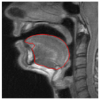
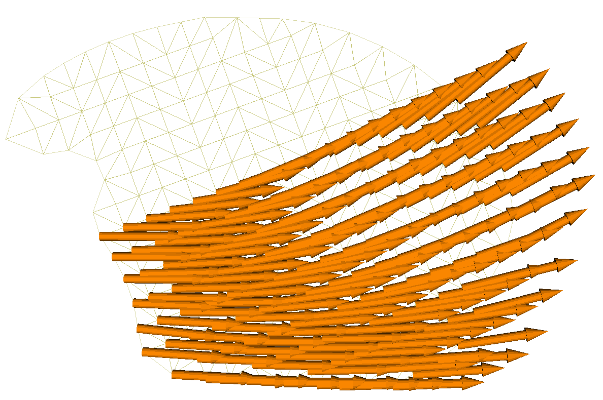
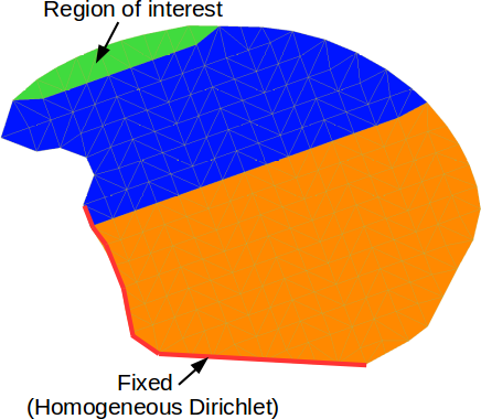
In the first example, we focus on the case study for the activation of the posterior genio-glossus (GGp), that is a lingual muscle located at the root of the tongue and inserted in the front to the mandible. The activation of this muscle compresses the tongue in the lower part and generates a forward and upward movement of the tongue body, because of the incompressibility of tongue tissues, for example during the production of the phonemes /i/ or /s/. The 2D mesh used in this example has been derived from the generic 3D mesh presented in [17] where the authors developed a process to generate subject-specific meshes. More precisely an automatic atlas-based method was proposed that generates subject-specific meshes via a registration guided by Magnetic Resonance Imaging. The domain $\Omega$ is depicted in Figure 1 (left). The width and height of the tongue are respectively equal to $73.8$ mm and $53.7$ mm. For the passive tissue material properties, we use the values reported in [48] based on indentation experiments on a cadaver’s tongue. The authors initially proposed an incompressible two parameter Yeoh hyperelastic material model and fitted the material constants to the data. In this work, a linear elastic material model is assumed. According to [125], linearisation of the model proposed in [48] yields $E$ $\simeq$ $6c10$ $=0.6$ MPa. For the sake of simplicity Poisson ratio is assumed to be $\nu=0.4$. No volumic force field is applied: ${\bf f}={\bf 0}$. The direction of the fibers ${\bf e}_{A}$ is depicted in Figure 1 (center) and corresponds approximately to the posterior genioglossus muscle [17]. Other parameters for fiber activation have been chosen as $T$ = 2e-5 MPa and $\beta=1$. The tongue is attached to the hyoid bone and to the mandible, which are supposed to be fixed. This leads to a homogeneous Dirichlet boundary condition such as depicted in Figure 1 (right). On the remaining part of the boundary a homogeneous Neumann condition (${\bf F}={\bf 0}$) is applied. The orange part depicts the region $\omega_{A}$ where fibers are supposed to be located. The green part depicts the region of interest $\omega$ for the computation of $J_{1}$ and $J_{2}$.

Figure 1: Tongue model: initial geometry (left), fiber orientation (center) and region of interest (right).

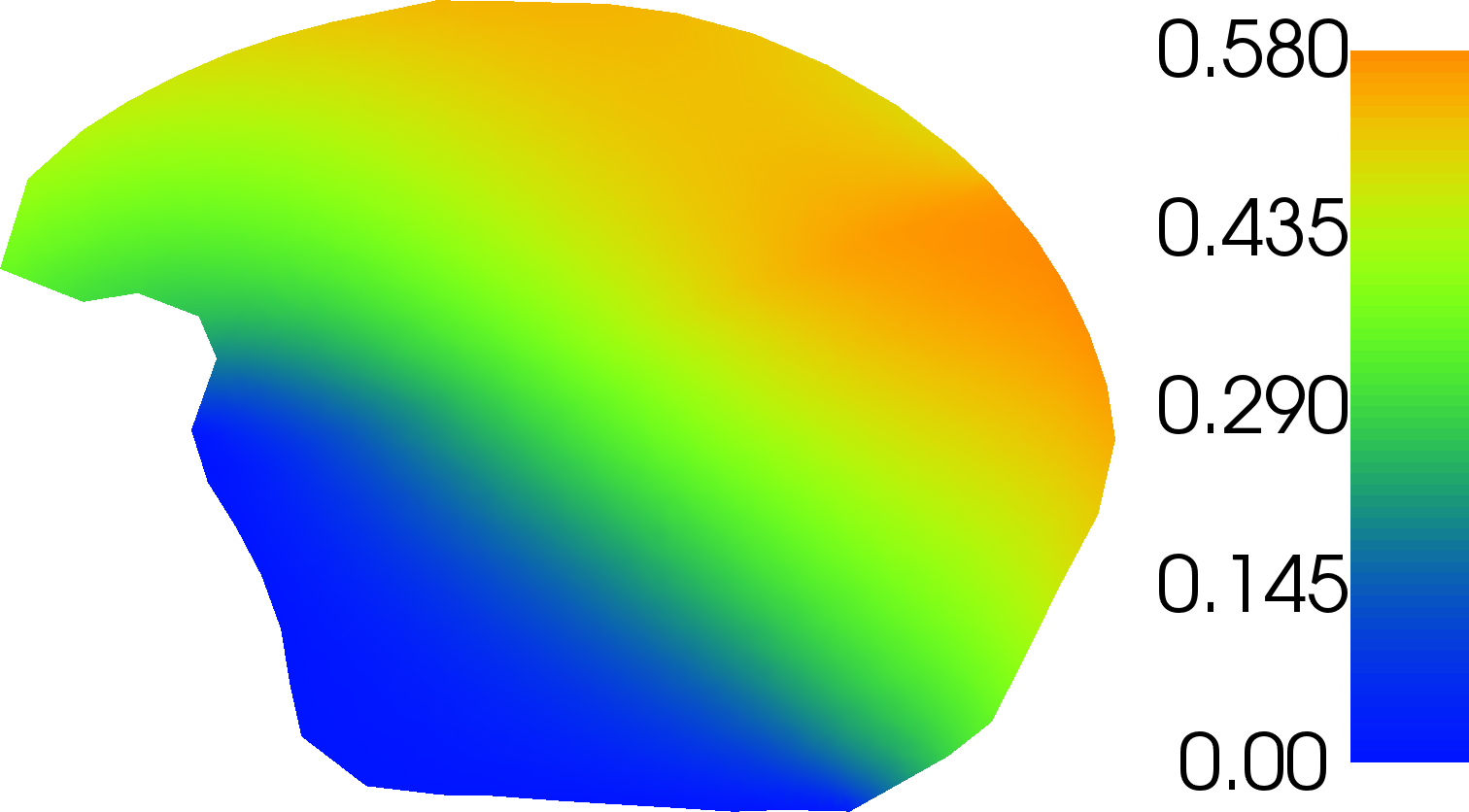
The resulting displacement is depicted in Figure 2 (left). We computed the relative displacement and the strain intensity, which maximal values are of 5.7 $\%$ and 4.8 $\%$, respectively: thus the small displacement and small strain assumptions are both verified in this case. The parameter $T$ has been chosen accordingly in order to respect these assumptions. In Figure 2, the dual solutions for the quantities of interest $J_{1}$ (center) and $J_{2}$ (right) are represented. As mentioned in Remark 2.1, the dual solution $z$ is used as a weight in the computation of the estimators, and influences the local refinement.

Figure 2: Tongue model: displacement (left), dual solutions for $J_{1}$ (center) and for $J_{2}$ (right).

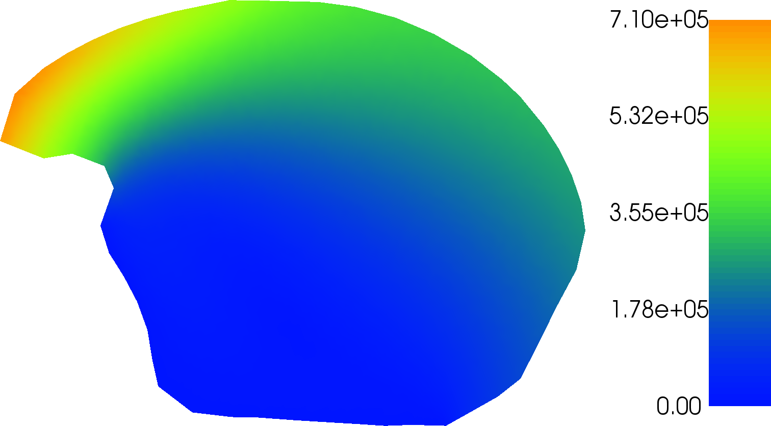
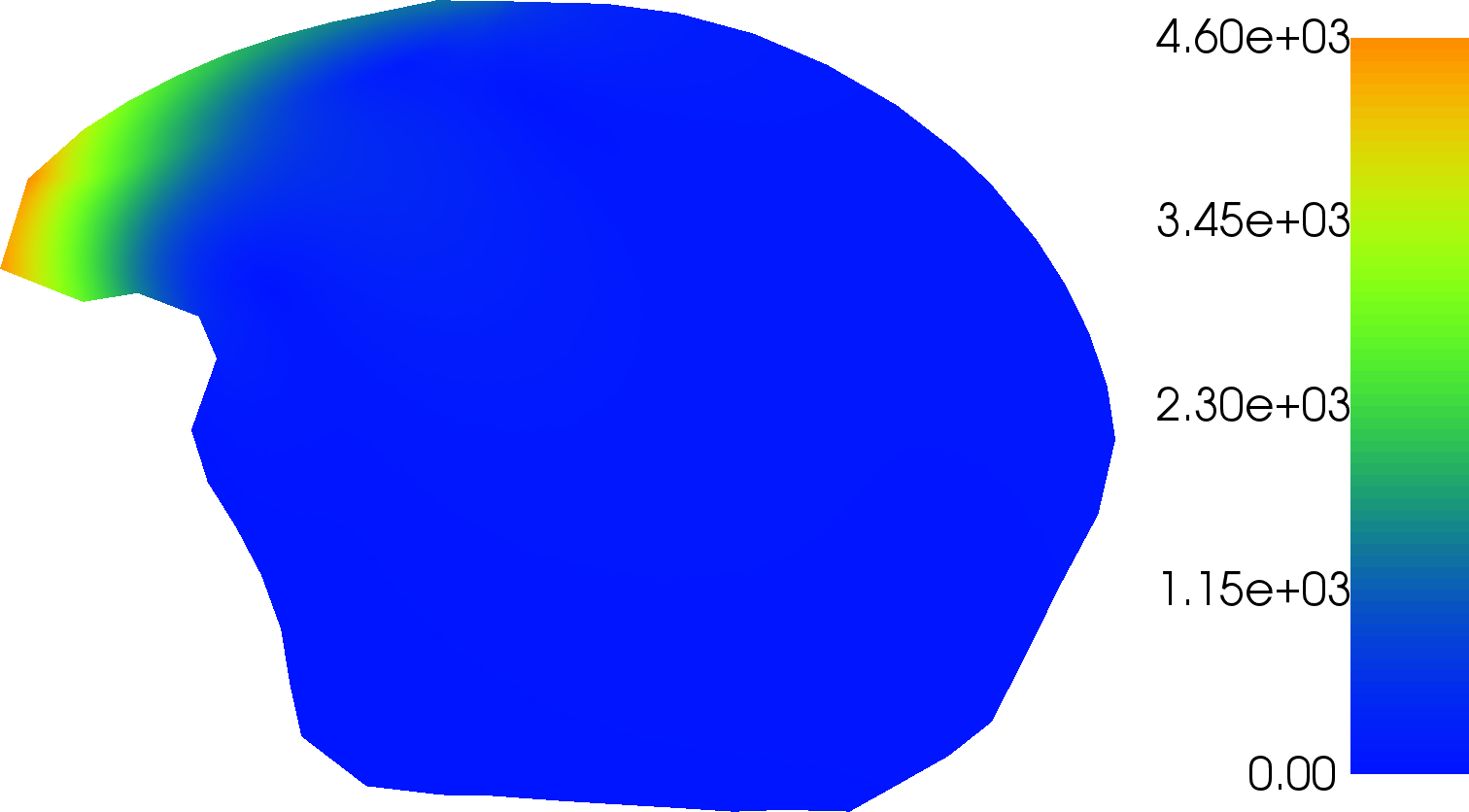
We present the final mesh after 2 and 8 iterations of Algorithm 1 for both quantities of interest $J_{1}$ and $J_{2}$, in Figure 3 and Figure 4, respectively. We first remark that the refinement occurs in some specific regions such as those near Dirichlet-Neumann transitions and concavities on the boundary. Note as well that the refinement is stronger for $J_{2}$ at the boundary of the region of interest $\omega$,.

Figure 3: Tongue mesh: refinement driven by the QoI $J_{1}$. Initial mesh (left) with 426 cells and a relative error of 1.07e-2, adapted meshes after 2 iterations (center) with 523 cells and a relative error of 2.82e-3 and after 8 iterations (right) with 5143 cells and a relative error of 3.82e-05.

Figure 4: Tongue mesh: refinement driven by the QoI $J_{2}$. Initial mesh (left) with 426 cells and a relative error of 2.51e-2, adapted meshes after 2 iterations (center) with 766 cells and a relative error of 2.21e-3 and after 8 iterations (right) with 13513 cells and a relative error of 2.44e-5.

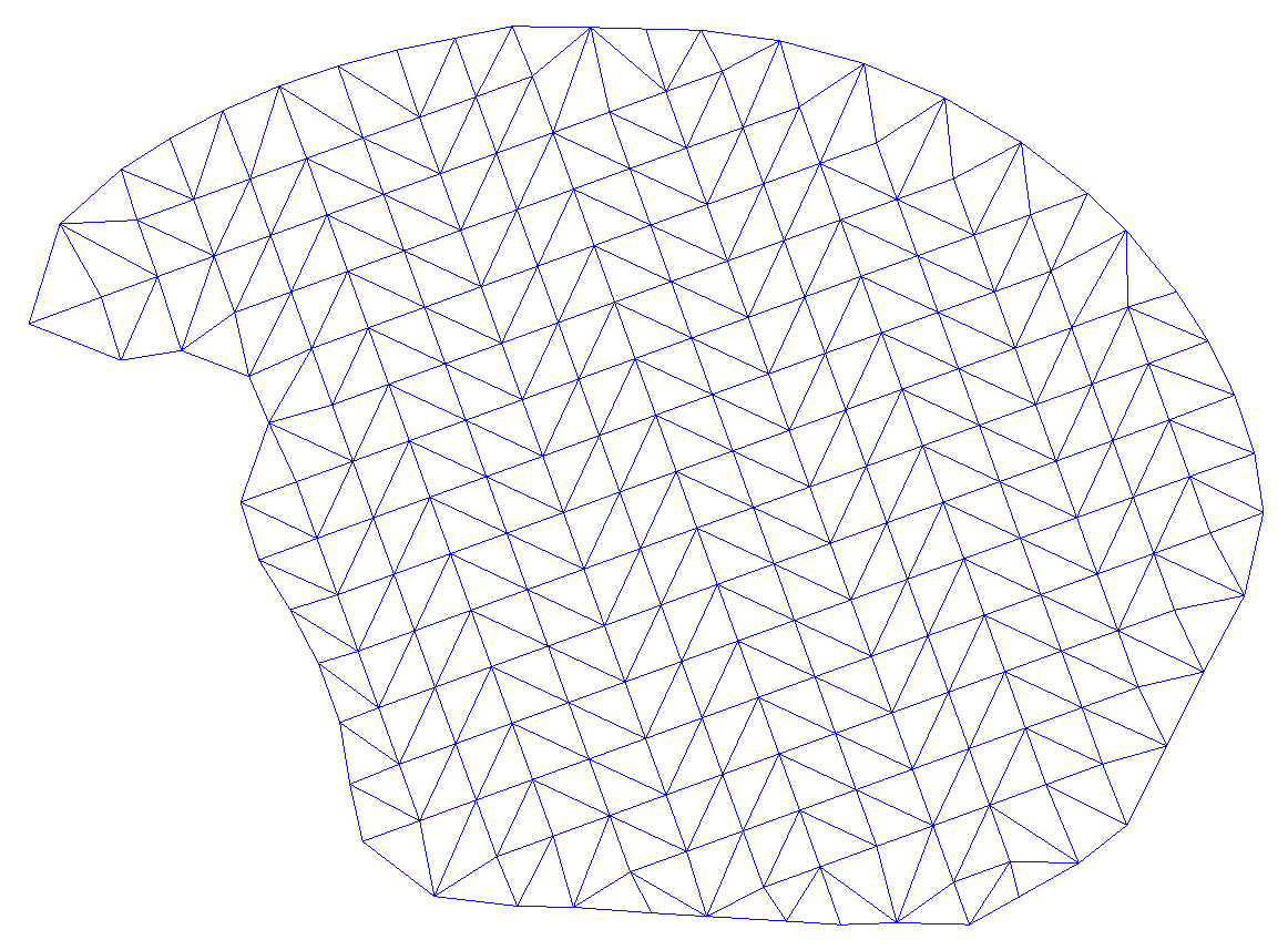
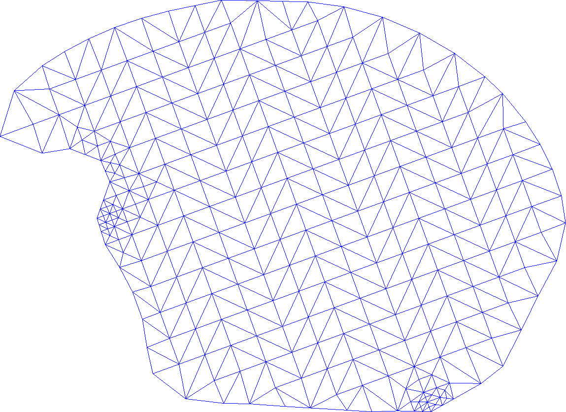
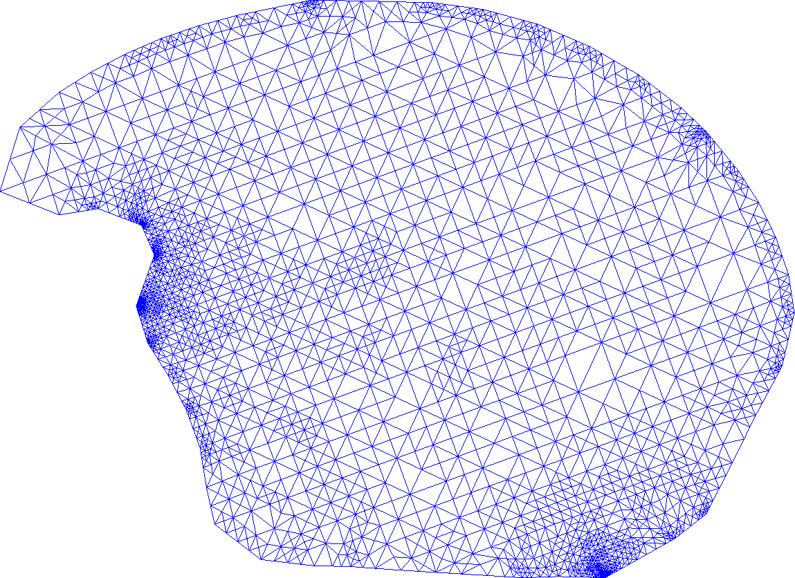
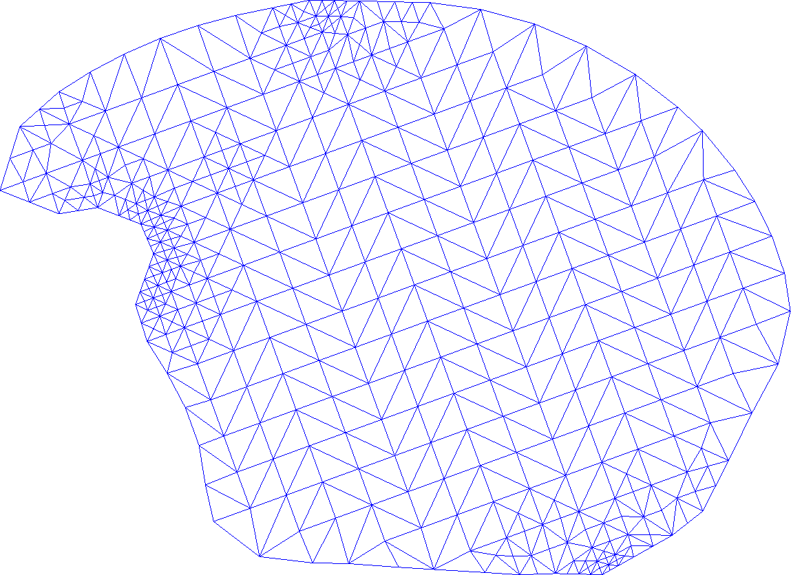
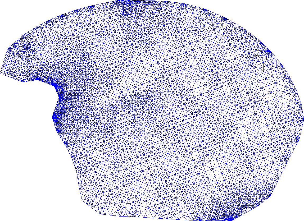
Figure 5 depicts the relative goal-oriented errors $|J_{1}({\bf u})-J_{1}({\bf u}_{h})|/|J_{1}({\bf u})|$ (left) and $|J_{2}({\bf u})-J_{2}({\bf u}_{h})|/|J_{2}({\bf u})|$ (right) versus $N$, the number of cells of the mesh, both for uniform refinement (blue) and adaptive refinement (red). The stopping criterion $\varepsilon$ has been fixed to 2e-4 and 1e-6, respectively. In each situation, we observe that, as expected, adaptive refinement performs better: not only it leads to a lower error but it also converges much faster when the number of cells $N$ is increased.

Figure 5: Tongue model: relative error for the QoI $J_{1}$ (left) and $J_{2}$ (right) vs. the number $N$ of cells in the case of uniform (blue) and adaptive (red) refinement.

Finally in Figure 6 we depict the efficiency indices for the global estimator $\eta_{h}$ and the sum of local estimators $\sum_{K}\eta_{K}$. For both quantities $J_{1}$ and $J_{2}$, the two estimators provide an estimation of the discretization error with an efficiency index around 1. In the case of $J_{2}$, we observe a slight overestimation for $\sum_{K}\eta_{K}$ and a slight underestimation for $\eta_{h}$.

Figure 6: Tongue model: efficiency indexes for $\eta_{h}$ (blue) and $\sum_{K}\eta_{K}$ vs. the number $N$ of cells for the QoI $J_{1}$ (left) and $J_{2}$ (right).

3.2 Human artery with fiber activation

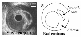
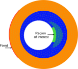
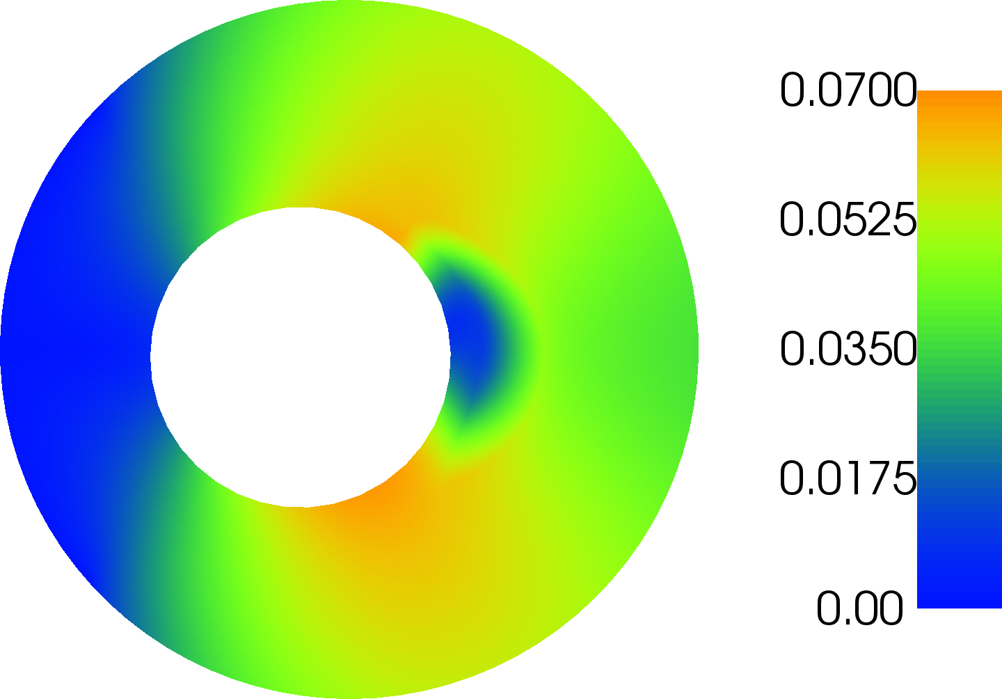
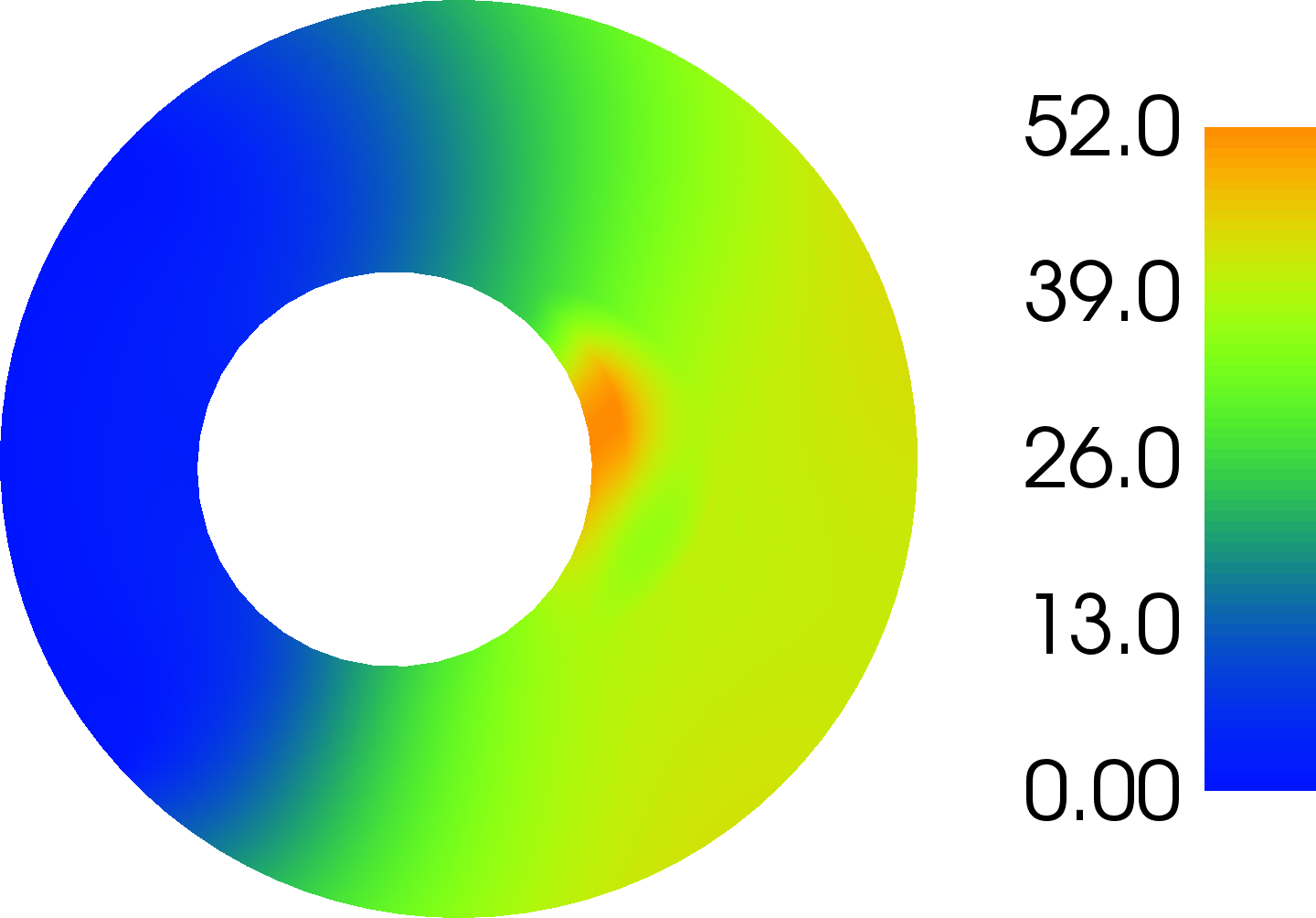
As a second example we showcase the performance of the proposed algorithm for the analysis of the mechanical response of an artery with vulnerable coronary plaque to internal loading. Rupture of the cap induces the formation of a thrombus which may obstruct the coronary artery, cause an acute syndrome and the patient death. The geometry (see Figure 7 (left)) comes from [70] where the authors develop a methodology to reconstruct the thickness of the necrotic core area and the calcium area as well as the Young’s moduli of the calcium, the necrotic core and the fibrosis. Their objective is the prediction of the vulnerable coronary plaque rupture. As represented in Figure 7 (left), the diameter of the Fibrosis is equal to 5 mm. Following [70], we set different elastic parameters in each region: $E=0.011$ MPa, $\nu=0.4$ in the necrotic core and $E=0.6$ MPa, $\nu=0.4$ in the surrounding tissue. No volumetric force field is applied: ${\bf f}={\bf 0}$. We consider muscle fibers only in the media layer, where smooth muscle cells are supposed to be perfectly oriented in the circumferential direction ${\bf e}_{A}={\bf e}_{\theta}$, where $({\bf e}_{r},{\bf e}_{\theta})$ is the basis for polar coordinates, see Figure 7 (center). Other parameters for fiber activation have been chosen as $T=0.01$ MPa and $\beta=1$. As depicted in Figure 7 (right), the artery is fixed on the red portion of external boundary $\Gamma_{D}$. Elsewhere, on the remaining part of the boundary, a homogeneous Neumann condition is applied: ${\bf F}={\bf 0}$. In the same figure, the green part represents the region of interest $\omega$. This choice is relevant in the study of vulnerable coronary plaque rupture. As in the previous example, we computed the relative displacement and the strain intensity, which maximal values are of 6.15 $\%$ and 0.3 $\%$, respectively. This ensures that small displacement and small strain assumptions are verified. Figure 8 depicts the magnitude of the solution in terms of displacements (left) and the dual solutions associated to $J_{1}$ (center) and $J_{2}$ (right).

Figure 7: Artery model: geometry (left), fiber orientation (center) and region of interest (right).

Figure 8: Artery model: displacement (left), dual solution for $J_{1}$ (center) and for $J_{2}$ (right).

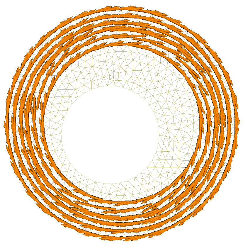
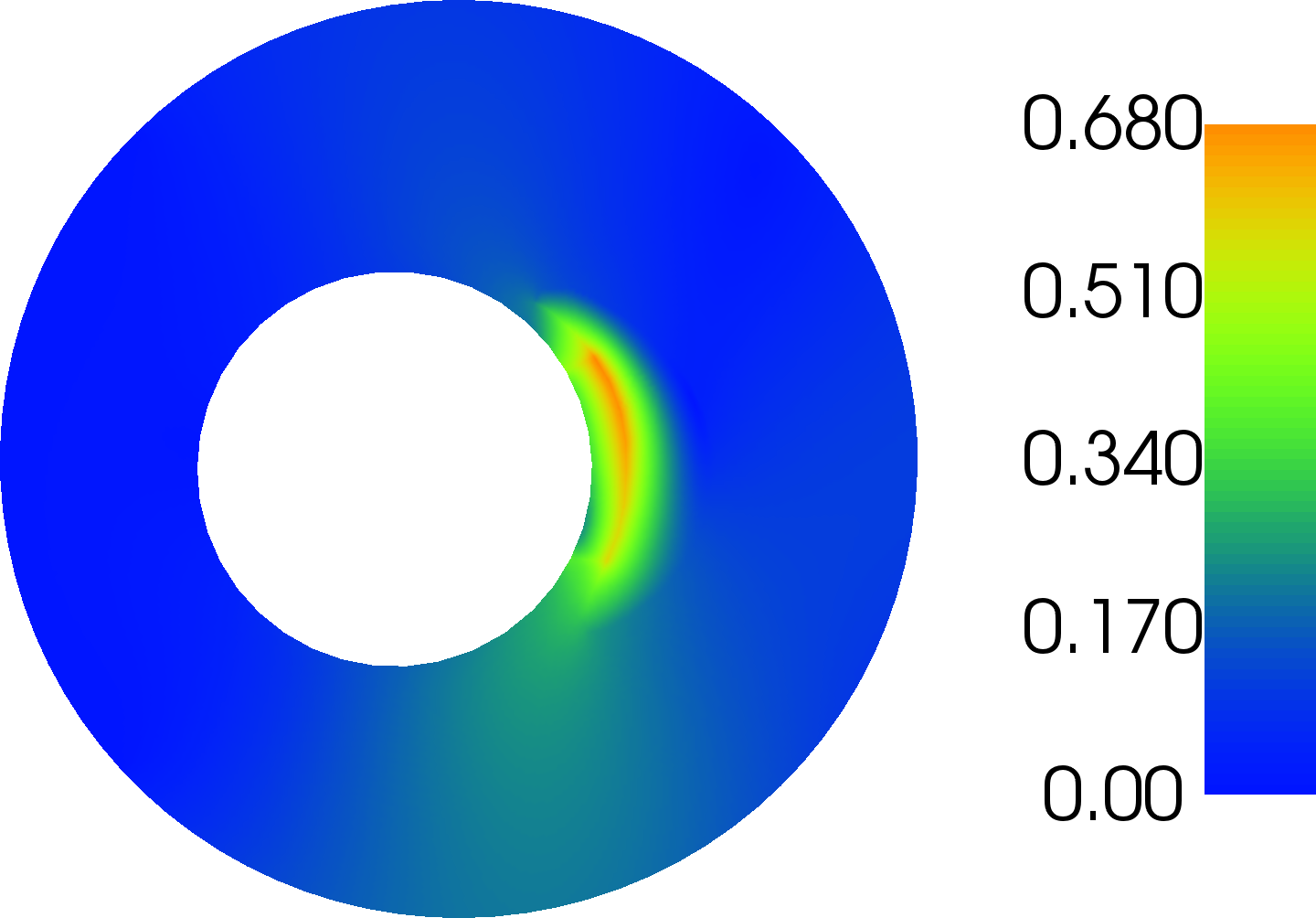
In Figure 9, we present the final mesh after 2 and 6 iterations of Algorithm 1 for the quantity of interest $J_{1}$. As in the previous example, the refinement occurs in some specific regions, such as those near Dirichlet-Neumann transitions and concavities on the boundary. Our results also show that the proposed method leads to the strong refinement near the interface between the necrotic core and the fibrosis, where stresses are localized because of the material heterogeneity. Conversely to the previous example, the refined meshes obtained for $J_{2}$ (not depicted) are very similar to those obtained for $J_{1}$.

Figure 9: Artery mesh: refinement driven by the QoI $J_{1}$. Initial mesh (left) with 1242 cells and a relative error of 3.83e-1, adapted meshes after 2 iterations (center) with 2079 cells and a relative error of 5.25e-2 and after 6 iterations (right) with 15028 cells and a relative error of 3.37e-3.

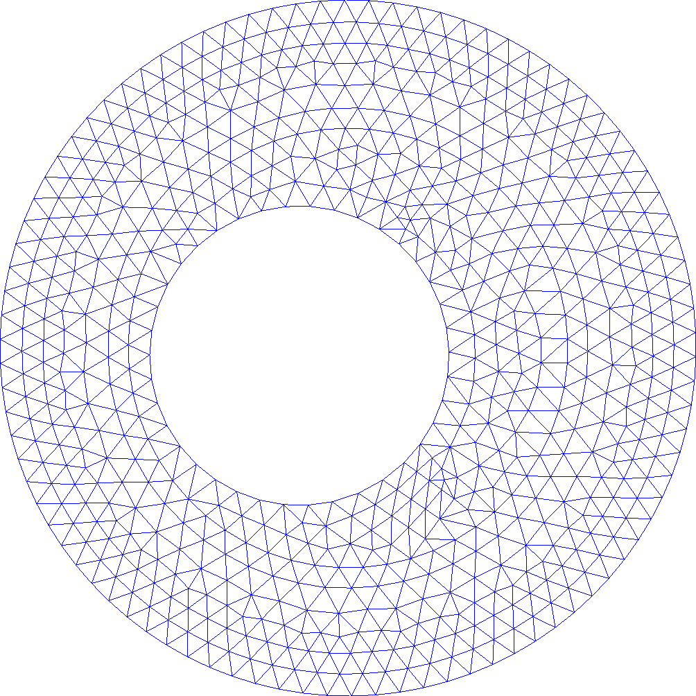
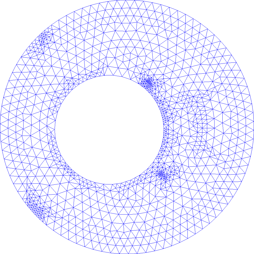
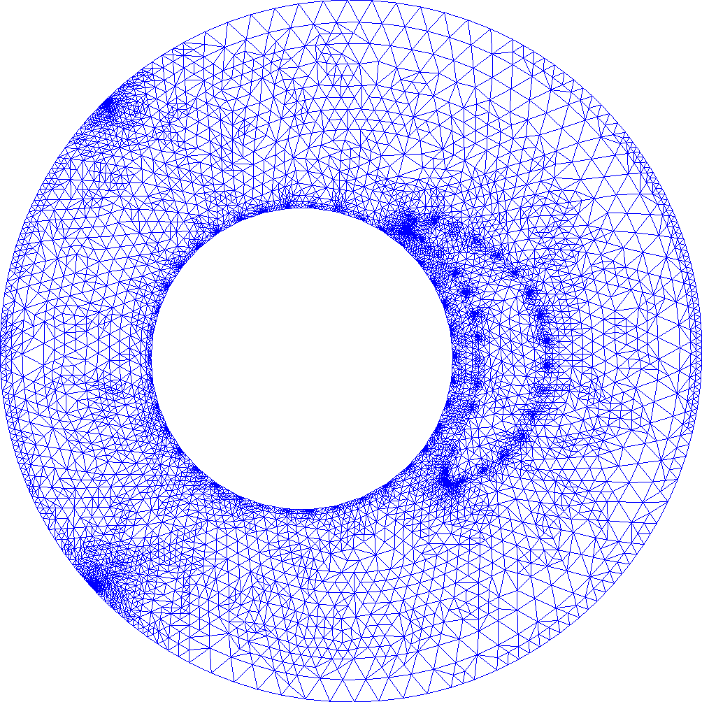
Figure 10 (left) depicts the relative goal-oriented error $|J_{1}({\bf u})-J_{1}({\bf u}_{h})|/|J_{1}({\bf u})|$ versus the number $N$ of cells in the mesh, both for uniform refinement (blue) and adaptive refinement (red). The stopping criterion $\varepsilon$ has been fixed at 5e-6. In Figure 10 (right), we depict the efficiency indices for the global estimator $\eta_{h}$ and the sum of local estimators $\sum_{K}\eta_{K}$. The same observations as in the previous example can be stated, and the estimators provide acceptable value of the discretization error. Moreover $\eta_{h}$ performs better though it still underestimates slightly the error. Results we obtained for the quantity $J_{2}$ are very similar.

Figure 10: Artery model. Left: relative error for the QoI $J_{1}$ vs. the number $N$ of cells in the case of uniform (blue) and adaptive (red) refinement. Right: efficiency indexes of $\eta_{h}$ (blue) and $\sum_{K}\eta_{K}$ vs. the number of cells $N$ for the QoI $J_{1}$.

4 Discussion

In the first part, we discuss about the ability of the proposed methodology to assess and reduce the discretization error. In a second part, we comment on some further issues to improve and guarantee the accuracy of the error estimator, and to optimize the mesh refinement algorithm. Finally we address the issue of tackling more complex problems that arise in current practice for clinical biomechanics, and point out the main limitations of the current study as well as some perspectives.

4.1 Towards quantification of the discretization error: first achievements

The numerical results obtained in the last section show the ability of the proposed framework to provide relevant information about the discretization error: though the global estimator $\eta_{h}$ provides only an approximation of the error in the quantity of interest $|J({\bf u})-J({\bf u}_{h})|$, this is often sufficient in practice. Moreover, the local estimators $\eta_{K}$ provide a means to evaluate “relative” errors and thereby drive mesh refinement (Algorithm 1). Both the local and global errors can be significantly reduced without much computational effort. For instance, in the first test-case 3.1, and for $J_{1}$, the error is reduced by a factor of almost 4, after two successive refinements, and with only 20 $\%$ of extra cells. In order to quantify more precisely the computational gains provided by the adaptive procedure, the computational time required to compute the error estimator and to regenerate or adapt the mesh should be thoroughly computed and analyzed, as was done for three-dimensional fracture problems treated by enriched finite element methods [62].

Let us emphasize the well-known fact that sources of discretization errors are local, and concentrated mostly in regions where the solution is not smooth, e.g. subjected to strong variations, discontinuities or singularities. As a consequence, uniform refinement is highly suboptimal, while adaptive refinement performs much better by optimizing the number of elements, their size and location within the domain. Moreover, the proposed adaptive procedure is fully automatic, and no a priori knowledge of the critical regions is needed. For goal-oriented error estimation, the refined mesh obtained by the algorithm can in fact be counter-intuitive, because it is driven by the sensitivity of the quantity of interest with respect to the local error. This sensitivity is obtained by solving the dual problem (see for instance Figure 2 in Section 3.1) whose solution is, indeed, often not intuitive and difficult to interpret from a physical viewpoint.

In comparison to widespread error techniques implemented in most of commercial finite element software, the DWR technique allows to estimate and to improve the error for an arbitrary quantity of interest $J$. Each practitioner can choose the relevant quantity of interest $J$ and obtain an approximation of the error on this quantity of interest $|J({\bf u})-J({\bf u}_{h})|$, as well as a map of the local error. The authors emphasize that the results obtained in the current study also demonstrate that the optimal refinement strategy depends significantly on the choice of the quantity of interest $J$. In general, such a goal-oriented refinement strategy leads to meshes which may differ significantly from those obtained by minimizing the error in energy. Remark that such goal-oriented approaches were also developed for the Zienkiewicz-Zhu error estimators [132] in [52, 53] and for explicit residual based estimates in [112] and [130].

4.2 Some further mathematical / computational issues

It is desired that the global estimator $\eta_{h}$ provide reliable information on the error in the quantity of interest $|J({\bf u})-J({\bf u}_{h})|$, providing quality measures to the user. In theory, this error is a guaranteed upper bound, with an explicit constant equal to $1$. Yet, the theory assumes that the dual solution $z$ is exactly known. This is never the case in practice as the dual problem is also solved using finite elements. Our numerical experiments show, however, that $|J({\bf u})-J({\bf u}_{h})|$ is estimated with reasonable accuracy and that the effectivity indices are close to 1, meaning that the approximate error on the quantity of interest is close to the (unknown) exact error on this quantity.

The numerical experiments provided in this paper confirm those of the literature on DWR technique, e.g., [14, 50, 110] showing that the DWR is, in most situations, a reliable approach to compute goal-oriented error estimates. However, in certain situations, the DWR estimator is not as reliable as desired, since the effect of approximating the dual solution is difficult to control. This issue has been already pointed in the literature: see e.g. [29, 93, 4] and earlier considerations in, e.g., [50, 10]. Especially, in [93] a simple situation where $\eta_{h}$ provides a poor estimation on a coarse mesh is detailed. There is up to now no simple, cheap and general technique to address this issue, but first solutions have been suggested in [29, 93, 4]. They consist in modifying the DWR estimator so as to take into account the approximation of $z$. This is a stimulating perspective for further research. Moreover, the issue of computing a cheaper approximation of $z$, without compromising the reliability and efficiency of the estimator still needs to be addressed in depth.

Concerning mesh refinement, though the local estimator $\eta_{K}$ combined with Algorithm 1 provides acceptable results, no effort has been spent on finding the value of parameter $\alpha$ in the Dörfler marking that yields improved refined meshes. On this topic, our global strategy for error estimation and mesh refinement is only a first attempt, and can be improved. For instance, in [12], an adaptive method based on specific weighting of the residuals of the primal and dual problems has been designed, and leads to quasi-optimal adapted meshes. Such a method could be tested and compared to the current one.

4.3 Applicability for patient-specific biomechanics?

Though the preliminary results presented in this paper demonstrate the relevance and practicability of a posteriori error estimators for providing quality control in quantities of interest to the biomechanics practitioner, and to drive mesh adaptation, much effort is still needed for the approaches developed here to address practical, personalized, clinically-relevant Finite Element (FE) simulations for biomechanical applications.

First, the compressible linear framework considered here is inadequate in practice and must be replaced by a fully non-linear, incompressible, time and history dependent model [98]. Non-linearities also occur due to boundary conditions, when, for instance, contact is present [33]. Moreover, most of the quantities of interest in biomechanics are non-linear (norm of the displacements, local shear stress, maximum admissible stress and strain, etc). It is important to point out here that the DWR method for goal-oriented error estimation is already capable of tackling non-linearities: see, e.g., [14] for the general framework, and, e.g., [68, 129] for first applications in non-linear elasticity and [112] for fracture mechanics. Nevertheless, this non-linear framework needs to be adapted and tested in the specific case of hyperelastic soft-tissue.

The major limitation of our work is that it assumes that the mathematical model used to describe the biomechanics problem is able to reproduce the physical reality. Unfortunately, in general, selecting the proper mathematical model for a given biomechanics problem is probably the most challenging part of the simulation process. The large, and increasing, number of papers dealing with the choice of constitutive model, for example, testifies for this difficulty. For a wide range of problems, indeed, modeling errors are the most significant. Estimating rigorously and systematically the impact of these errors is extremely challenging, in particular when dealing with patient-specific simulations. Dealing with this issue is the focus of ongoing research in our teams but is far beyond the scope of this paper.

We would nonetheless like to make the following remarks. The first problem which must be addressed is the choice of a model (hyperelastic, viscous, porous, single/multi-scale…). The chosen model has parameters which must be estimated through inverse analysis. Once estimates, or probability distributions for these parameters are available, their importance on quantities of interest must be evaluated, through sensitivity analysis and uncertainty quantification. The major difficulty is, therefore, to select the proper model, and its parameters for a given patient. As in vivo experiments are in general not possible, data must be extracted as the patient is being treated, e.g. during an operation. This can be done using Bayesian methods, which provide a reconciliation between expert knowledge on patient cohorts (prior) and actual properties of a given patient [106, 105]. Real-time machine-learning-like methods such as Kalman filters demonstrated as well promising results [82, 57]. To evaluate the effects of uncertainties on such material parameters, accelerated Monte-Carlo methods are possible avenues of investigation [59]. An exciting question is the comparative usefulness and combination of physical models (potentially learnt during medical treatment) and machine-learning algorithms, mostly based on data acquired during the intervention. Last but not least, note that the DWR method is based on optimal control principles, that makes it suitable for extensions to parameter calibration (viewed as an optimal control problem). In such a setting, it allows to combine sensitivity analysis with goal-oriented a posteriori error estimation, see [15]. In the same spirit, the interplay between a posteriori error estimation and uncertainty quantification has been object of recent research interests [40, 56].

We also note that if users can obtain some estimate, even rough, of modeling errors, they will also be able to compare discretization and model errors. This enables the coarsening of the mesh if the discretization error is unnecessarily small in comparison to the modeling error as is done, e.g. in [5] and [120, 23, 121, 118, 122] for adaptive scale selection. Conversely, for specific applications where modeling errors are small or moderate, the mesh can be refined efficiently to increase the precision.

With our methodology, practitioners spending a large amount of time and effort in patient-specific mesh generation can obtain useful information on the impact of the quality of the mesh on quantities of interest to them. This information goes well beyond purely geometrical criteria for the regularity of the elements which are typically provided in commercial software.

This information can be used directly to optimize the choice of the discretization/mesh in view of minimizing the error on a specific quantity of interest. Fast/real-time numerical methods which provide real-time predictions have been intensively researched since the beginning of the 1990’s. Those approaches are critical to build surgical planning and guidance tools, for example. Reliable error estimation is critical in these situations to guarantee the accuracy, but has been extremely scarcely addressed in the literature. As a first step in this direction, the recent work of [25] provides a real-time mesh refinement algorithm for needle insertion. Mesh refinement is driven by a ZZ error estimate, for the global norm. It would be interesting to extend such a method for goal-oriented error estimation, e.g. on the motion of a target, or reaction/friction force along the needle shaft.

We should also mention alternative approaches to (implicit, standard) finite elements for fast nonlinear finite element analysis: for instance the solution of total lagrangian formulation of the equilibrium equations on graphics processing unit for neurosurgical simulation [64, 63, 65], or model order reduction techniques for the real-time, interactive simulation of tissue tearing during laparoscopic surgery [90, 91, 103]. A perspective consists in extending the current framework to such numerical methods where error control is particularly challenging. For explicit approaches, the interplay between the choice of the time-step and that of the mesh size is a difficult topic, especially for domains with significant stiffness differences where adaptive and multi-time-step schemes should be investigated.

References

-
Abbas et al. [2017]
Abbas, M., Ern, A., Pignet, N., 2017. Hybrid High-Order methods for finite
deformations of hyperelastic materials, preprint (hal-01575370).
URL https://hal.archives-ouvertes.fr/hal-01575370 - Adams [1975] Adams, R. A., 1975. Sobolev spaces. Academic Press, New York-London, pure and Applied Mathematics, Vol. 65.
Ainsworth and Oden [2000]
Ainsworth, M., Oden, J. T., 2000. A posteriori error estimation in finite
element analysis. Pure and Applied Mathematics. Wiley-Interscience, New York.
URL http://dx.doi.org/10.1002/9781118032824 -
Ainsworth and Rankin [2012]
Ainsworth, M., Rankin, R., 2012. Guaranteed computable bounds on quantities of
interest in finite element computations. International Journal for Numerical
Methods in Engineering 89 (13), 1605–1634.
URL http://dx.doi.org/10.1002/nme.3276 - Akbari Rahimabadi et al. [2015] Akbari Rahimabadi, A., Kerfriden, P., Bordas, S., 2015. Scale selection in nonlinear fracture mechanics of heterogeneous materials. Philosophical Magazine 95 (28-30), 3328–3347.
Al-Dirini et al. [2016]
Al-Dirini, R. M. A., Reed, M. P., Hu, J., Thewlis, D., Sep. 2016. Development
and Validation of a High Anatomical Fidelity FE Model for the
Buttock and Thigh of a Seated Individual. Annals of Biomedical
Engineering 44 (9), 2805–2816.
URL https://link.springer.com/article/10.1007/s10439-016-1560-3 - Alliez et al. [2005] Alliez, P., Cohen-Steiner, D., Yvinec, M., Desbrun, M., 2005. Variational tetrahedral meshing. ACM Transactions on Graphics 24, 617–625, sIGGRAPH ’2005 Conference Proceedings.
Avril et al. [2010]
Avril, S., Badel, P., Duprey, A., 2010. Anisotropic and hyperelastic
identification of in vitro human arteries from full-field optical
measurements. Journal of Biomechanics 43 (15), 2978 – 2985.
URL http://www.sciencedirect.com/science/article/pii/S0021929010003738 -
Badel et al. [2013]
Badel, P., Rohan, C. P.-Y., Avril, S., Oct. 2013. Finite Element simulation
of buckling-induced vein tortuosity and influence of the wall constitutive
properties. Journal of the Mechanical Behavior of Biomedical Materials
26 (Supplement C), 119–126.
URL http://www.sciencedirect.com/science/article/pii/S175161611300163X -
Bangerth and Rannacher [2003]
Bangerth, W., Rannacher, R., 2003. Adaptive finite element methods for
differential equations. Lectures in Mathematics ETH Zürich. Birkhäuser
Verlag, Basel.
URL http://dx.doi.org/10.1007/978-3-0348-7605-6 - BaniHani and De [2009] BaniHani, S. M., De, S., 2009. A comparison of some model order reduction methods for fast simulation of soft tissue response using the point collocation-based method of finite spheres. Engineering with Computers 25 (1), 37–47.
Becker et al. [2011]
Becker, R., Estecahandy, E., Trujillo, D., 2011. Weighted marking for
goal-oriented adaptive finite element methods. SIAM Journal on Numerical
Analysis 49 (6), 2451–2469.
URL http://dx.doi.org/10.1137/100794298 - Becker and Rannacher [1996] Becker, R., Rannacher, R., 1996. A feed-back approach to error control in finite element methods: basic analysis and examples. East-West Journal of Numerical Mathematics 4 (4), 237–264.
Becker and Rannacher [2001]
Becker, R., Rannacher, R., 2001. An optimal control approach to a posteriori
error estimation in finite element methods. Acta Numerica 10, 1–102.
URL http://dx.doi.org/10.1017/S0962492901000010 -
Becker and Vexler [2005]
Becker, R., Vexler, B., 2005. Mesh refinement and numerical sensitivity
analysis for parameter calibration of partial differential equations. Journal
of Computational Physics 206 (1), 95–110.
URL http://dx.doi.org/10.1016/j.jcp.2004.12.018 - Beirão da Veiga et al. [2016] Beirão da Veiga, L., Brezzi, F., Marini, L., Russo, A., 2016. Virtual element method for general second-order elliptic problems on polygonal meshes. Mathematical Models and Methods in Applied Sciences 26 (04), 729–750.
- Bijar et al. [2016] Bijar, A., Rohan, P.-Y., Perrier, P., Payan, Y., 2016. Atlas-based automatic generation of subject-specific finite element tongue meshes. Annals of Biomedical Engineering 44 (1), 16–34.
- Bommes et al. [2013] Bommes, D., Lévy, B., Pietroni, N., Puppo, E., Silva, C., Tarini, M., Zorin, D., 2013. Quad-mesh generation and processing: A survey. In: Computer Graphics Forum. Vol. 32. Wiley Online Library, pp. 51–76.
- Bordas et al. [2010] Bordas, S. P. A., Rabczuk, T., Rodenas, J., Kerfriden, P., Moumnassi, M., Belouettar, S., 2010. Recent advances towards reducing the meshing and re-meshing burden in computational sciences. In: Topping, B. H. V., Adam, J. M. and Pallares, F. J. eds. Computational technology reviews, Vol. 2. Saxe-Coburg Publications, pp. 51-82.
Bro-Nielsen and Cotin [1996]
Bro-Nielsen, M., Cotin, S., Aug. 1996. Real-time Volumetric Deformable
Models for Surgery Simulation using Finite Elements and
Condensation. Computer Graphics Forum 15 (3), 57–66.
URL http://onlinelibrary.wiley.com/doi/10.1111/1467-8659.1530057/abstract -
Buchaillard et al. [2007]
Buchaillard, S., Brix, M., Perrier, P., Payan, Y., Sep. 2007. Simulations of
the consequences of tongue surgery on tongue mobility: implications for
speech production in post-surgery conditions. The International Journal of
Medical Robotics and Computer Assisted Surgery 3 (3), 252–261.
URL http://onlinelibrary.wiley.com/doi/10.1002/rcs.142/abstract - Bucki et al. [2011] Bucki, M., Lobos, C., Payan, Y., Hitschfeld, N., 2011. Jacobian-based repair method for finite element meshes after registration. Engineering with Computers 27 (3), 285–297.
- Budarapu et al. [2014] Budarapu, P. R., Gracie, R., Yang, S.-W., Zhuang, X., Rabczuk, T., 2014. Efficient coarse graining in multiscale modeling of fracture. Theoretical and Applied Fracture Mechanics 69, 126–143.
- Budninskiy et al. [2016] Budninskiy, M., Liu, B., De Goes, F., Tong, Y., Alliez, P., Desbrun, M., 2016. Optimal voronoi tessellations with hessian-based anisotropy. ACM Transactions on Graphics (TOG) 35 (6), 242.
- Bui et al. [2018] Bui, H. P., Tomar, S., Courtecuisse, H., Cotin, S., Bordas, S. P. A., March 2018. Real-time error control for surgical simulation. IEEE Transactions on Biomedical Engineering 65 (3), 596–607.
Burkhart et al. [2013]
Burkhart, T. A., Andrews, D. M., Dunning, C. E., May 2013. Finite element
modeling mesh quality, energy balance and validation methods: A review with
recommendations associated with the modeling of bone tissue. Journal of
Biomechanics 46 (9), 1477–1488.
URL http://www.sciencedirect.com/science/article/pii/S0021929013001383 -
Burman et al. [2015]
Burman, E., Claus, S., Hansbo, P., Larson, M. G., Massing, A., 2015. CutFEM:
discretizing geometry and partial differential equations. International
Journal for Numerical Methods in Engineering 104 (7), 472–501.
URL http://dx.doi.org/10.1002/nme.4823 -
Buttin et al. [2013]
Buttin, R., Zara, F., Shariat, B., Redarce, T., Grangé, G., Aug. 2013.
Biomechanical simulation of the fetal descent without imposed theoretical
trajectory. Computer Methods and Programs in Biomedicine 111 (2), 389–401.
URL http://www.sciencedirect.com/science/article/pii/S0169260713001132 -
Carstensen [2005]
Carstensen, C., 2005. Estimation of higher Sobolev norm from lower order
approximation. SIAM Journal on Numerical Analysis 42 (5), 2136–2147.
URL http://dx.doi.org/10.1137/S0036142902413615 - Chau et al. [2017] Chau, K. N., Chau, K. N., Ngo, T., Hackl, K., Nguyen-Xuan, H., 2017. A polytree-based adaptive polygonal finite element method for multi-material topology optimization. Computer Methods in Applied Mechanics and Engineering.
- Chen et al. [2017] Chen, L., Wei, H., Wen, M., 2017. An interface-fitted mesh generator and virtual element methods for elliptic interface problems. Journal of Computational Physics 334, 327–348.
- Cotin et al. [1999] Cotin, S., Delingette, H., Ayache, N., Jan. 1999. Real-time elastic deformations of soft tissues for surgery simulation. IEEE Transactions on Visualization and Computer Graphics 5 (1), 62–73.
- Courtecuisse et al. [2014] Courtecuisse, H., Allard, J., Kerfriden, P., Bordas, S. P., Cotin, S., Duriez, C., 2014. Real-time simulation of contact and cutting of heterogeneous soft-tissues. Medical Image Analysis 18 (2), 394–410.
- Couteau et al. [2000] Couteau, B., Payan, Y., Lavallée, S., 2000. The Mesh-Matching algorithm: an automatic 3D mesh generator for finite element structures. Journal of Biomechanics 33, 1005–1009.
- Cowin and Humphrey [2001] Cowin, S. C., Humphrey, J. D., 2001. Cardiovascular soft tissue mechanics. Springer.
- Davydov and Schaback [2016] Davydov, O., Schaback, R., 2016. Optimal stencils in Sobolev spaces. arXiv preprint arXiv:1611.04750.
- De et al. [2005] De, S., Kim, J., Lim, Y.-J., Srinivasan, M. A., 2005. The point collocation-based method of finite spheres (PCMFS) for real time surgery simulation. Computers & Structures 83 (17), 1515–1525.
Di Pietro and Ern [2015]
Di Pietro, D. A., Ern, A., 2015. A hybrid high-order locking-free method for
linear elasticity on general meshes. Computer Methods in Applied Mechanics
and Engineering 283, 1–21.
URL http://dx.doi.org/10.1016/j.cma.2014.09.009 -
Dörfler [1996]
Dörfler, W., 1996. A convergent adaptive algorithm for Poisson’s
equation. SIAM Journal on Numerical Analysis 33 (3), 1106–1124.
URL http://dx.doi.org/10.1137/0733054 -
Eigel et al. [2016]
Eigel, M., Merdon, C., Neumann, J., 2016. An adaptive multilevel Monte
Carlo method with stochastic bounds for quantities of interest with
uncertain data. SIAM/ASA Journal on Uncertainty Quantification 4 (1),
1219–1245.
URL http://dx.doi.org/10.1137/15M1016448 -
Eriksson et al. [1995]
Eriksson, K., Estep, D., Hansbo, P., Johnson, C., 1995. Introduction to
adaptive methods for differential equations. In: Acta numerica, 1995. Acta
Numer. Cambridge Univ. Press, Cambridge, pp. 105–158.
URL http://dx.doi.org/10.1017/S0962492900002531 -
Ern and Guermond [2004]
Ern, A., Guermond, J.-L., 2004. Theory and practice of finite elements. Vol.
159 of Applied Mathematical Sciences. Springer-Verlag, New York.
URL http://dx.doi.org/10.1007/978-1-4757-4355-5 - Francis et al. [2017] Francis, A., Ortiz-Bernardin, A., Bordas, S., Natarajan, S., 2017. Linear smoothed polygonal and polyhedral finite elements. International Journal for Numerical Methods in Engineering 109 (9), 1263–1288.
Franquet et al. [2013]
Franquet, A., Avril, S., Le Riche, R., Badel, P., Schneider, F. C., Boissier,
C., Favre, J.-P., Nov. 2013. Identification of the in vivo elastic properties
of common carotid arteries from MRI: A study on subjects with and without
atherosclerosis. Journal of the Mechanical Behavior of Biomedical Materials
27 (Supplement C), 184–203.
URL http://www.sciencedirect.com/science/article/pii/S1751616113001045 -
Frey and George [2008]
Frey, P. J., George, P.-L., 2008. Mesh generation, 2nd Edition. ISTE, London;
John Wiley & Sons, Inc., Hoboken, NJ, application to finite elements.
URL http://dx.doi.org/10.1002/9780470611166 - Fries et al. [2017] Fries, T., Omerović, S., Schöllhammer, D., Steidl, J., 2017. Higher-order meshing of implicit geometries. Part I: Integration and interpolation in cut elements. Computer Methods in Applied Mechanics and Engineering 313, 759–784.
George et al. [2016]
George, P. L., Borouchaki, H., Barral, N., 2016. Geometric validity (positive
jacobian) of high-order lagrange finite elements, theory and practical
guidance. Engineering with Computers 32 (3), 405–424.
URL http://dx.doi.org/10.1007/s00366-015-0422-1 -
Gerard et al. [2005]
Gerard, J. M., Ohayon, J., Luboz, V., Perrier, P., Payan, Y., Dec. 2005.
Non-linear elastic properties of the lingual and facial tissues assessed by
indentation technique: Application to the biomechanics of speech
production. Medical Engineering & Physics 27 (10), 884–892.
URL http://www.sciencedirect.com/science/article/pii/S1350453305001888 - Geuzaine and Remacle [2009] Geuzaine, C., Remacle, J.-F., 2009. Gmsh: A 3-D finite element mesh generator with built-in pre-and post-processing facilities. International Journal for Numerical Methods in Engineering 79 (11), 1309–1331.
Giles and Süli [2002]
Giles, M. B., Süli, E., 2002. Adjoint methods for PDEs: a posteriori error
analysis and postprocessing by duality. Acta Numerica 11, 145–236.
URL http://dx.doi.org/10.1017/S096249290200003X -
Goel et al. [2007]
Goel, V. K., Mehta, A., Jangra, J., Faizan, A., Kiapour, A., Hoy, R. W., Fauth,
A. R., Feb. 2007. Anatomic Facet Replacement System (AFRS)
Restoration of Lumbar Segment Mechanics to Intact: A Finite
Element Study and In Vitro Cadaver Investigation. SAS Journal
1 (1), 46–54.
URL http://www.ncbi.nlm.nih.gov/pmc/articles/PMC4365566/ - González-Estrada et al. [2014] González-Estrada, O. A., Nadal, E., Ródenas, J., Kerfriden, P., Bordas, S. P.-A., Fuenmayor, F., 2014. Mesh adaptivity driven by goal-oriented locally equilibrated superconvergent patch recovery. Computational Mechanics 53 (5), 957–976.
- González-Estrada et al. [2015] González-Estrada, O. A., Ródenas, J. J., Bordas, S. P., Nadal, E., Kerfriden, P., Fuenmayor, F. J., 2015. Locally equilibrated stress recovery for goal oriented error estimation in the extended finite element method. Computers & Structures 152, 1–10.
Gras et al. [2012]
Gras, L.-L., Mitton, D., Viot, P., Laporte, S., Nov. 2012. Hyper-elastic
properties of the human sternocleidomastoideus muscle in tension. Journal of
the Mechanical Behavior of Biomedical Materials 15 (Supplement C), 131–140.
URL http://www.sciencedirect.com/science/article/pii/S1751616112001804 -
Grätsch and Bathe [2005]
Grätsch, T., Bathe, K.-J., Jan. 2005. A posteriori error estimation
techniques in practical finite element analysis. Computers & Structures
83 (4), 235–265.
URL http://www.sciencedirect.com/science/article/pii/S0045794904003165 -
Guignard et al. [2016]
Guignard, D., Nobile, F., Picasso, M., 2016. A posteriori error estimation for
elliptic partial differential equations with small uncertainties. Numerical
Methods for Partial Differential Equations. An International Journal 32 (1),
175–212.
URL http://dx.doi.org/10.1002/num.21991 - Haouchine et al. [2013] Haouchine, N., Dequidt, J., Peterlik, I., Kerrien, E., Berger, M.-O., Cotin, S., 2013. Image-guided simulation of heterogeneous tissue deformation for augmented reality during hepatic surgery. In: Mixed and Augmented Reality (ISMAR), 2013 IEEE International Symposium on. IEEE, pp. 199–208.
Haslinger and Renard [2009]
Haslinger, J., Renard, Y., 2009. A new fictitious domain approach inspired by
the extended finite element method. SIAM Journal on Numerical Analysis
47 (2), 1474–1499.
URL http://dx.doi.org/10.1137/070704435 - Hauseux et al. [2017] Hauseux, P., Hale, J. S., Bordas, S. P., 2017. Accelerating monte carlo estimation with derivatives of high-level finite element models. Computer Methods in Applied Mechanics and Engineering 318, 917–936.
- Hu and Zhang [2016] Hu, K., Zhang, Y. J., 2016. Centroidal voronoi tessellation based polycube construction for adaptive all-hexahedral mesh generation. Computer Methods in Applied Mechanics and Engineering 305, 405–421.
- Ito et al. [2009] Ito, Y., Shih, A., Soni, B., 2009. Octree-based reasonable-quality hexahedral mesh generation using a new set of refinement templates. International Journal for Numerical Methods in Engineering 77 (13), 1809–1833.
- Jin et al. [2017] Jin, Y., González-Estrada, O., Pierard, O., Bordas, S., 2017. Error-controlled adaptive extended finite element method for 3d linear elastic crack propagation. Computer Methods in Applied Mechanics and Engineering 318, 319–348.
Joldes et al. [2009a]
Joldes, G. R., Wittek, A., Miller, K., 2009a. Non-locking
tetrahedral finite element for surgical simulation. Communications in
Numerical Methods in Engineering 25 (7), 827–836.
URL http://onlinelibrary.wiley.com/doi/10.1002/cnm.1185/abstract -
Joldes et al. [2009b]
Joldes, G. R., Wittek, A., Miller, K., 2009b. Suite of finite
element algorithms for accurate computation of soft tissue deformation for
surgical simulation. Medical Image Analysis 13 (6), 912–919.
URL http://www.sciencedirect.com/science/article/pii/S1361841508001424 -
Joldes et al. [2010]
Joldes, G. R., Wittek, A., Miller, K., 2010. Real-time nonlinear finite element
computations on GPU – Application to neurosurgical simulation. Computer
Methods in Applied Mechanics and Engineering 199 (49–52), 3305–3314.
URL http://www.sciencedirect.com/science/article/pii/S0045782510002045 - Kalameh et al. [2016] Kalameh, H. A., Pierard, O., Friebel, C., Béchet, E., 2016. Semi-implicit representation of sharp features with level sets. Finite Elements in Analysis and Design 117, 31–45.
- Kraus and Steinmann [2017] Kraus, M., Steinmann, P., 2017. Finite element formulations for 3d convex polyhedra in nonlinear continuum mechanics. Computer Assisted Methods in Engineering and Science 19 (2), 121–134.
Larsson et al. [2002]
Larsson, F., Hansbo, P., Runesson, K., 2002. Strategies for computing
goal-oriented a posteriori error measures in non-linear elasticity.
International Journal for Numerical Methods in Engineering 55 (8), 879–894.
URL http://dx.doi.org/10.1002/nme.513 -
Laville et al. [2009]
Laville, A., Laporte, S., Skalli, W., Jul. 2009. Parametric and
subject-specific finite element modelling of the lower cervical spine.
Influence of geometrical parameters on the motion patterns. Journal of
Biomechanics 42 (10), 1409–1415.
URL http://www.jbiomech.com/article/S0021929009002073/abstract - Le Floc’h et al. [2009] Le Floc’h, S., Ohayon, J., Tracqui, P., Finet, G., Gharib, A. M., Maurice, R. L., Cloutier, G., Pettigrew, R. I., Jul. 2009. Vulnerable Atherosclerotic Plaque Elasticity Reconstruction Based on a Segmentation-Driven Optimization Procedure Using Strain Measurements: Theoretical Framework. IEEE Transactions on Medical Imaging 28 (7), 1126–1137.
- Lee et al. [2017] Lee, C.-K., Mihai, L. A., Hale, J. S., Kerfriden, P., Bordas, S. P., 2017. Strain smoothing for compressible and nearly-incompressible finite elasticity. Computers & Structures 182, 540–555.
- Li et al. [2016] Li, M., Miller, K., Joldes, G. R., Kikinis, R., Wittek, A., 2016. Biomechanical model for computing deformations for whole-body image registration: A meshless approach. International Journal for Numerical Methods in Biomedical Engineering 32 (12).
- Lim and De [2004] Lim, Y.-J., De, S., 2004. On the use of meshfree methods and a geometry based surgical cutting algorithm in multimodal medical simulations. In: Haptic Interfaces for Virtual Environment and Teleoperator Systems, 2004. HAPTICS’04. Proceedings. 12th International Symposium on. IEEE, pp. 295–301.
- Lim and De [2007] Lim, Y.-J., De, S., 2007. Real time simulation of nonlinear tissue response in virtual surgery using the point collocation-based method of finite spheres. Computer Methods in Applied Mechanics and Engineering 196 (31), 3011–3024.
- Liu et al. [2016] Liu, Y., Saputra, A., Song, C., 2016. Stress analysis of stl models by octree mesh and scaled boundary finite element method. In: Mechanics of Structures and Materials XXIV: Proceedings of the 24th Australian Conference on the Mechanics of Structures and Materials (ACMSM24, Perth, Australia, 6-9 December 2016). CRC Press, p. 351.
- Lobos et al. [2010] Lobos, C., Payan, Y., Hitschfeld, N., 2010. Techniques for the generation of 3D Finite Element Meshes of human organs. Informatics in Oral Medicine: Advanced Techniques in Clinical and Diagnostic Technologies. Hershey, PA: Medical Information Science Reference, 126–158.
- Loerakker et al. [2011] Loerakker, S., Manders, E., Strijkers, G. J., Nicolay, K., Baaijens, F. P., Bader, D. L., Oomens, C. W., 2011. The effects of deformation, ischemia, and reperfusion on the development of muscle damage during prolonged loading. Journal of Applied Physiology 111 (4), 1168–1177.
- Logg et al. [2012] Logg, A., Mardal, K.-A., Wells, G. N., et al., 2012. Automated Solution of Differential Equations by the Finite Element Method. Springer.
Luboz et al. [2017]
Luboz, V., Bailet, M., Boichon Grivot, C., Rochette, M., Diot, B., Bucki, M.,
Payan, Y., Jun. 2017. Personalized modeling for real-time pressure ulcer
prevention in sitting posture. Journal of Tissue Viability.
URL http://www.sciencedirect.com/science/article/pii/S0965206X17300918 -
Maday and Patera [2000]
Maday, Y., Patera, A. T., 2000. Numerical analysis of a posteriori finite
element bounds for linear functional outputs. Mathematical Models and Methods
in Applied Sciences 10 (5), 785–799.
URL http://dx.doi.org/10.1142/S0218202500000409 - Moës et al. [2003] Moës, N., Cloirec, M., Cartraud, P., Remacle, J.-F., 2003. A computational approach to handle complex microstructure geometries. Computer Methods in Applied Mechanics and Engineering 192 (28), 3163–3177.
Moireau et al. [2009]
Moireau, P., Chapelle, D., Le Tallec, P., 2009. Filtering for distributed
mechanical systems using position measurements: perspectives in medical
imaging. Inverse Problems 25 (3), 035010, 25.
URL http://dx.doi.org/10.1088/0266-5611/25/3/035010 - Mouly et al. [2017] Mouly, Q., Evrard, F., van Wachem, B., Denner, F., 2017. Minimizing finite-volume discretization errors on polyhedral meshes. Bulletin of the American Physical Society.
- Moumnassi et al. [2011] Moumnassi, M., Belouettar, S., Béchet, É., Bordas, S. P., Quoirin, D., Potier-Ferry, M., 2011. Finite element analysis on implicitly defined domains: An accurate representation based on arbitrary parametric surfaces. Computer Methods in Applied Mechanics and Engineering 200 (5), 774–796.
- Moumnassi et al. [2014] Moumnassi, M., Bordas, S. P. A., Figueredo, R., Sansen, P., 2014. Analysis using higher-order xfem: implicit representation of geometrical features from a given parametric representation. Mechanics & Industry 15 (5), 443–448.
- Natarajan et al. [2017a] Natarajan, S., Francis, A., Atroshchenko, E., Bordas, S., 2017a. A new one point quadrature rule over arbitrary star convex polygon/polyhedron. arXiv preprint arXiv:1707.00399.
- Natarajan et al. [2017b] Natarajan, S., Ooi, E. T., Saputra, A., Song, C., 2017b. A scaled boundary finite element formulation over arbitrary faceted star convex polyhedra. Engineering Analysis with Boundary Elements 80, 218–229.
- Nguyen et al. [2008] Nguyen, V. P., Rabczuk, T., Bordas, S., Duflot, M., 2008. Meshless methods: a review and computer implementation aspects. Mathematics and Computers in Simulation 79 (3), 763–813.
- Nguyen-Hoang et al. [2017] Nguyen-Hoang, S., Sohn, D., Kim, H.-G., 2017. A new polyhedral element for the analysis of hexahedral-dominant finite element models and its application to nonlinear solid mechanics problems. Computer Methods in Applied Mechanics and Engineering 324, 248–277.
Niroomandi et al. [2012]
Niroomandi, S., Alfaro, I., González, D., Cueto, E., Chinesta, F., 2012.
Real-time simulation of surgery by reduced-order modeling and X-FEM
techniques. International Journal for Numerical Methods in Biomedical
Engineering 28 (5), 574–588.
URL http://onlinelibrary.wiley.com/doi/10.1002/cnm.1491/abstract -
Niroomandi et al. [2013]
Niroomandi, S., González, D., Alfaro, I., Bordeu, F., Leygue, A., Cueto, E.,
Chinesta, F., 2013. Real-time simulation of biological soft tissues: a PGD
approach. International Journal for Numerical Methods in Biomedical
Engineering 29 (5), 586–600.
URL http://onlinelibrary.wiley.com/doi/10.1002/cnm.2544/abstract -
Nochetto et al. [2009a]
Nochetto, R. H., Siebert, K. G., Veeser, A., 2009a. Theory of
adaptive finite element methods: an introduction. In: Multiscale, nonlinear
and adaptive approximation. Springer, Berlin, pp. 409–542.
URL {}{}}{http://dx.doi.org/10.1007/978-3-642-03413-8_12}{cmtt} -
Nochetto et~al. [2009b]
Nochetto, R.~H., Veeser, A., Verani, M., 2009b. A safeguarded dual
weighted residual method. IMA Journal of Numerical Analysis 29~(1), 126--140.
URL http://dx.doi.org/10.1093/imanum/drm026 - Ong et~al. [2015] Ong, T.~H., Heaney, C.~E., Lee, C.-K., Liu, G., Nguyen-Xuan, H., 2015. On stability, convergence and accuracy of bes-fem and bfs-fem for nearly incompressible elasticity. Computer Methods in Applied Mechanics and Engineering 285, 315--345.
Paraschivoiu and Patera [1998]
Paraschivoiu, M., Patera, A.~T., 1998. A hierarchical duality approach to
bounds for the outputs of partial differential equations. Computer Methods in
Applied Mechanics and Engineering 158~(3-4), 389--407.
URL http://dx.doi.org/10.1016/S0045-7825(99)00270-4 -
Paraschivoiu et~al. [1997]
Paraschivoiu, M., Peraire, J., Patera, A.~T., 1997. A posteriori finite element
bounds for linear-functional outputs of elliptic partial differential
equations. Computer Methods in Applied Mechanics and Engineering 150~(1-4),
289--312, symposium on Advances in Computational Mechanics, Vol. 2 (Austin,
TX, 1997).
URL http://dx.doi.org/10.1016/S0045-7825(97)00086-8 -
Park et~al. [2013]
Park, W.~M., Kim, K., Kim, Y.~H., Sep. 2013. Effects of degenerated
intervertebral discs on intersegmental rotations, intradiscal pressures, and
facet joint forces of the whole lumbar spine. Computers in Biology and
Medicine 43~(9), 1234--1240.
URL http://www.sciencedirect.com/science/article/pii/S0010482513001613 - Payan and Ohayon [2017] Payan, Y., Ohayon, J., 2017. Biomechanics of living organs : hyperelastic constitutive laws for finite element modeling. Academic press series in biomedical engineering.
- Pellerin et~al. [2017] Pellerin, J., Johnen, A., Remacle, J.-F., 2017. Combining tetrahedra into hexahedra: a vertex based strategy. arXiv preprint arXiv:1705.02451.
Perrin et~al. [2015]
Perrin, D., Badel, P., Orgéas, L., Geindreau, C., Dumenil, A., Albertini,
J.-N., Avril, S., Jul. 2015. Patient-specific numerical simulation of
stent-graft deployment: Validation on three clinical cases. Journal of
Biomechanics 48~(10), 1868--1875.
URL http://www.sciencedirect.com/science/article/pii/S0021929015002511 -
Pierrat et~al. [2014]
Pierrat, B., Molimard, J., Navarro, L., Avril, S., Calmels, P., Jun. 2014.
Evaluation of the mechanical efficiency of knee orthoses: A combined
experimental–numerical approach. Proceedings of the Institution of
Mechanical Engineers, Part H: Journal of Engineering in Medicine 228~(6),
533--546.
URL https://doi.org/10.1177/0954411914533944 -
Prudhomme and Oden [1999]
Prudhomme, S., Oden, J.~T., 1999. On goal-oriented error estimation for
elliptic problems: application to the control of pointwise errors. Computer
Methods in Applied Mechanics and Engineering 176~(1-4), 313--331, new
advances in computational methods (Cachan, 1997).
URL http://dx.doi.org/10.1016/S0045-7825(98)00343-0 -
Quesada et~al. [????]
Quesada, C., Alfaro, I., González, D., Chinesta, F., Cueto, E., ???? Haptic
simulation of tissue tearing during surgery. International Journal for
Numerical Methods in Biomedical EngineeringIn press.
URL http://onlinelibrary.wiley.com/doi/10.1002/cnm.2926/abstract - Rajagopal et~al. [????] Rajagopal, A., Kraus, M., Steinmann, P., ???? Hyperelastic analysis based on a polygonal finite element method. Mechanics of Advanced Materials and Structures~(just-accepted), in press.
- Rappel et~al. [2017] Rappel, H., Beex, L.~A., Bordas, S.~P., 2017. Bayesian inference to identify parameters in viscoelasticity. Mechanics of Time-Dependent Materials, 1--38.
- Rappel et~al. [2016] Rappel, H., Beex, L.~A., Hale, J.~S., Bordas, S., 2016. Bayesian inference for the stochastic identification of elastoplastic material parameters: Introduction, misconceptions and insights. arXiv preprint arXiv:1606.02422.
- Ray et~al. [2017] Ray, N., Sokolov, D., Reberol, M., Ledoux, F., Lévy, B., 2017. Hexahedral meshing: Mind the gap!Preprint (hal-01551603).
- Remacle [2017] Remacle, J.-F., 2017. A two-level multithreaded delaunay kernel. Computer-Aided Design 85, 2--9.
- Ródenas et~al. [2013] Ródenas, J., Giovannelli, L., Nadal, E., Navarro, J., Tur, M., 2013. Creation of patient specific finite element models of bone-prosthesis—simulation of the effect of future implants. Computational Vision and Medical Image Processing IV: VIPIMAGE 2013, 161.
Rognes and Logg [2013]
Rognes, M.~E., Logg, A., 2013. Automated goal-oriented error control I:
Stationary variational problems. SIAM Journal on Scientific Computing
35~(3), C173--C193.
URL http://dx.doi.org/10.1137/10081962X -
Romo et~al. [2014]
Romo, A., Badel, P., Duprey, A., Favre, J.-P., Avril, S., Feb. 2014. In vitro
analysis of localized aneurysm rupture. Journal of Biomechanics 47~(3),
607--616.
URL http://www.sciencedirect.com/science/article/pii/S0021929013006398 - Rüter et~al. [2013] Rüter, M., Gerasimov, T., Stein, E., 2013. Goal-oriented explicit residual-type error estimates in xfem. Computational Mechanics 52~(2), 361--376.
Schmidt et~al. [2012]
Schmidt, H., Galbusera, F., Rohlmann, A., Zander, T., Wilke, H.-J., 2012.
Effect of multilevel lumbar disc arthroplasty on spine kinematics and facet
joint loads in flexion and extension: a finite element analysis. European
Spine Journal 21~(5), 663--674.
URL https://link.springer.com/article/10.1007/s00586-010-1382-1 - Sellam et~al. [2017] Sellam, M., Natarajan, S., Kannan, K., 2017. Smoothed polygonal finite element method for generalized elastic solids subjected to torsion. Computers & Structures 188, 32--44.
Shang et~al. [2017]
Shang, F., Gan, Y., Guo, Y., May 2017. Hexahedral mesh generation via
constrained quadrilateralization. PLoS ONE 12~(5).
URL http://www.ncbi.nlm.nih.gov/pmc/articles/PMC5436764/ - Shepherd and Johnson [2009] Shepherd, J., Johnson, C., 2009. Hexahedral mesh generation for biomedical models in scirun. Engineering with Computers 25, 97--114.
Shilo and Gefen [2012]
Shilo, M., Gefen, A., Jan. 2012. Identification of capillary blood pressure
levels at which capillary collapse is likely in a tissue subjected to large
compressive and shear deformations. Computer Methods in Biomechanics and
Biomedical Engineering 15~(1), 59--71.
URL http://dx.doi.org/10.1080/10255842.2010.539208 - Silani et~al. [2014] Silani, M., Ziaei-Rad, S., Talebi, H., Rabczuk, T., 2014. A semi-concurrent multiscale approach for modeling damage in nanocomposites. Theoretical and Applied Fracture Mechanics 74, 30--38.
- Talebi et~al. [2016] Talebi, H., Saputra, A., Song, C., 2016. Stress analysis of 3d complex geometries using the scaled boundary polyhedral finite elements. Computational Mechanics 58~(4), 697--715.
- Talebi et~al. [2013] Talebi, H., Silani, M., Bordas, S.~P., Kerfriden, P., Rabczuk, T., 2013. Molecular dynamics/xfem coupling by a three-dimensional extended bridging domain with applications to dynamic brittle fracture. International Journal for Multiscale Computational Engineering 11~(6).
- Talebi et~al. [2014] Talebi, H., Silani, M., Bordas, S.~P., Kerfriden, P., Rabczuk, T., 2014. A computational library for multiscale modeling of material failure. Computational Mechanics 53~(5), 1047--1071.
- Talebi et~al. [2015] Talebi, H., Silani, M., Rabczuk, T., 2015. Concurrent multiscale modeling of three dimensional crack and dislocation propagation. Advances in Engineering Software 80, 82--92.
Telfer et~al. [2016]
Telfer, S., Erdemir, A., Woodburn, J., Cavanagh, P.~R., Jan. 2016. Simplified
versus geometrically accurate models of forefoot anatomy to predict plantar
pressures: A finite element study. Journal of Biomechanics 49~(2),
289--294.
URL http://www.sciencedirect.com/science/article/pii/S0021929015007022 - Trabelsi et~al. [2015] Trabelsi, O., Davis, F.~M., Rodriguez-Matas, J.~F., Duprey, A., Avril, S., 2015. Patient specific stress and rupture analysis of ascending thoracic aneurysms. Journal of Biomechanics 48~(10), 1836--1843.
- Tracqui and Ohayon [2004] Tracqui, P., Ohayon, J., 2004. Transmission of mechanical stresses within the cytoskeleton of adherent cells: a theoretical analysis based on a multi-component cell model. Acta Biotheoretica 52~(4), 323--341.
- Tur et~al. [2015] Tur, M., Albelda, J., Marco, O., Ródenas, J.~J., 2015. Stabilized method of imposing dirichlet boundary conditions using a recovered stress field. Computer Methods in Applied Mechanics and Engineering 296, 352--375.
Verfürth [2013]
Verfürth, R., 2013. A posteriori error estimation techniques for finite
element methods. Numerical Mathematics and Scientific Computation. Oxford
University Press, Oxford.
URL http://dx.doi.org/10.1093/acprof:oso/9780199679423.001.0001 - Walton et~al. [2017] Walton, S., Hassan, O., Morgan, K., 2017. Advances in co-volume mesh generation and mesh optimisation techniques. Computers & Structures 181, 70--88.
Whiteley and Tavener [2014]
Whiteley, J.~P., Tavener, S.~J., 2014. Error estimation and adaptivity for
incompressible hyperelasticity. International Journal for Numerical Methods
in Engineering 99~(5), 313--332.
URL http://dx.doi.org/10.1002/nme.4677 - Wick [2016] Wick, T., 2016. Goal functional evaluations for phase-field fracture using PU-based DWR mesh adaptivity. Computational Mechanics 57~(6), 1017--1035.
Zhang et~al. [2007]
Zhang, Y., Bazilevs, Y., Goswami, S., Bajaj, C.~L., Hughes, T., May 2007.
Patient-Specific Vascular NURBS Modeling for Isogeometric
Analysis of Blood Flow. Computer Methods in Applied Mechanics and
Engineering 196~(29-30), 2943--2959.
URL http://www.ncbi.nlm.nih.gov/pmc/articles/PMC2839408/ -
Zienkiewicz and Zhu [1987]
Zienkiewicz, O.~C., Zhu, J.~Z., 1987. A simple error estimator and adaptive
procedure for practical engineering analysis. International Journal for
Numerical Methods in Engineering 24~(2), 337--357.
URL http://dx.doi.org/10.1002/nme.1620240206