Forward asteroseismic modeling of stars with a convective core from gravity-mode oscillations: parameter estimation and stellar model selection
Abstract
We propose a methodological framework to perform forward asteroseismic modeling of stars with a convective core, based on gravity-mode oscillations. These probe the near-core region in the deep stellar interior. The modeling relies on a set of observed high-precision oscillation frequencies of low-degree coherent gravity modes with long lifetimes and their observational uncertainties. Identification of the mode degree and azimuthal order is assumed to be achieved from rotational splitting and/or from period spacing patterns. This paper has two major outcomes. The first is a comprehensive list and discussion of the major uncertainties of theoretically predicted gravity-mode oscillation frequencies based on linear pulsation theory, caused by fixing choices of the input physics for evolutionary models. Guided by a hierarchy among these uncertainties of theoretical frequencies, we subsequently provide a global methodological scheme to achieve forward asteroseismic modeling. We properly take into account correlations amongst the free parameters included in stellar models. Aside from the stellar mass, metalicity and age, the major parameters to be estimated are the near-core rotation rate, the amount of convective core overshooting, and the level of chemical mixing in the radiative zones. This modeling scheme allows for maximum likelihood estimation of the stellar parameters for fixed input physics of the equilibrium models, followed by stellar model selection considering various choices of the input physics. Our approach uses the Mahalanobis distance instead of the often used statistic and includes heteroscedasticity. It provides estimation of the unknown variance of the theoretically predicted oscillation frequencies.
1 Introduction
Asteroseismology of low-mass stars with stochastically-excited pressure-mode oscillations often relies on simple scaling of solar oscillation frequencies. The so-called scaling relations are easy to apply and provide estimates of the stellar mass, radius, and age, assuming that the stars under consideration behave similarly to the Sun (e.g., Chaplin & Miglio, 2013; Hekker & Christensen-Dalsgaard, 2017, for reviews). If the aim is to improve the input physics of stellar models, however, one must go beyond application of scaling relations. This requires testing various assumptions and choices for the input physics that enters the computation of the stellar equilibrium models upon which one relies for the estimation of theoretical oscillation frequencies. In practice, estimation of various parameters that are left free in the computation of equilibrium models is required, along with proper error assessment. Subsequently, statistical model selection must be applied after the parameter estimation has been achieved, in order to evaluate the capacity of the input physics in explaining the asteroseismic data.
Approaches to achieve parameter estimation followed by evaluation of the input physics from stellar model selection in asteroseismology have been developed and improved, particularly since space photometry became available. An enlightening astrostatistics tutorial of various statistical methods for asteroseismology is available in Appourchaux (2014). Usually, parameter estimation is done from forward modeling by adopting a grid-based approach and considering millions of stellar structure models of different evolutionary stage. Early applications to low-mass stars with solar-like oscillations were made by, e.g., Miglio & Montalbán (2005); Quirion et al. (2010) and to subdwarfs by Brassard et al. (2001). In those studies, a comparison between observed and theoretically predicted frequencies was adopted to achieve the parameter estimation, while selection of the best model input physics among various choices was limited so far. Our focus is upon this latter aspect. Applications in the space asteroseismology era have so far also been focused on low-mass stars with solar-like oscillations (e.g., Gruberbauer et al., 2013; Appourchaux et al., 2014; Deheuvels et al., 2016; Bellinger et al., 2016; Silva Aguirre et al., 2017, to list a few) and on white dwarfs (e.g. Giammichele et al., 2017). Gruberbauer et al. (2012) developed a Bayesian framework that includes systematic uncertainties due to surface-effects that occur for solar-like oscillations (e.g., Ball & Gizon, 2017; Trampedach et al., 2017). The cause of this effect is unknown, yet it is dominant over other choices of the input physics when fitting oscillation frequencies and must therefore be treated properly. These unknown surface effects can be avoided by fitting frequency separations and ratios thereof, rather than the frequency values themselves. This has been done in most applications of solar-like oscillations so far.
The potential of the detected oscillations in terms of probing power is totally different for gravity modes than for pressure modes. The latter mainly probe envelope physics, while gravity modes dominantly probe near-core physics, and mixed modes in evolved stars have combined capacity. The exploitation of gravity-mode oscillations in stars born with a convective core and a radiative envelope (i.e., spectral type from early F to O) faces different challenges but offers new opportunities compared to solar-like oscillations. Gravity modes are strongly affected, and thus optimally suited to probe three phenomena in the deep stellar interior: convective core overshooting, near-core rotation and chemical mixing. The aim of the current paper is twofold: (i) to assess the major uncertainties in predicted theoretical frequencies for the case of gravity modes with long lifetime, leading to the requirement of heteroscedasticity in the statistical treatment; (ii) to provide a methodological framework for forward modeling, taking into account that gravity-mode oscillations depend non-linearly on the free parameters of stellar equilibrium models (e.g., Townsend & Teitler, 2013) and that these parameters are correlated (e.g., Fig. 11 in Pápics et al., 2014).
While thousands of low-mass stars were observed with mag level precision by Kepler (see, e.g., Chaplin & Miglio, 2013; Hekker & Christensen-Dalsgaard, 2017, for reviews), the satellite observed far fewer intermediate- and high-mass stars with gravity-mode oscillations, because the exoplanet hunting from planetary transits required observing a large sample of cool low-mass stars as potential hosts. For this reason, few stars with mass above 2 M⊙ in the Field-of-View of the nominal mission were monitored. Moreover, despite notable new detections of non-radial oscillations in tens of such stars made with the MOST (e.g., Walker et al., 2005; Saio et al., 2006; Aerts et al., 2006; Cameron et al., 2008; Zwintz et al., 2013) and CoRoT (e.g., Poretti et al., 2009; Neiner et al., 2009; Degroote et al., 2010; Briquet et al., 2011; Pápics et al., 2012; Zwintz et al., 2014) satellites, the time-series photometry assembled by these two missions was limited from weeks to a few months. While this is sufficient to detect gravity modes, it is often insufficient to identify them in terms of their spherical harmonic mode wavenumbers . Such mode identification is a necessary pre-requisite to model the interior physical properties of stars and to improve the input physics of theoretical models.
The bias towards asteroseismology of low-mass stars is also related to the time scales of the oscillations. Solar-like oscillations of low-mass stars are excited stochastically in their outer convective envelope and have periodicities ranging from minutes for the core-hydrogen burning phase to hours for red giants. This stands in sharp contrast to the coherent gravity modes with periods up to several days, leading to complex beating patterns among the modes that may cover several years (e.g., Kurtz et al., 2014; Saio et al., 2015; Van Reeth et al., 2015; Bowman et al., 2016; Pápics et al., 2017). Such modes are self-driven by a heat- or flux-blocking mechanism (e.g. Aerts et al., 2010, Chapters 2 and 3) and have lifetimes of tens to millions of years, i.e., long compared with the duration of the data sets (cf. Fig. 3 discussed below). Such gravity modes occur in stars with masses from roughly 1.4 to 40 . Our long-term aim to improve the evolutionary models of such intermediate- and high-mass stars using asteroseismology is motivated by the fact that they are the dominant suppliers of the chemicals in galaxies, while their evolution models are far more uncertain than those of low-mass stars.
The evolution of stars born with a well-developed convective core is appreciably affected by the size and properties of their convective core region, the interior rotation, and the transport of chemicals and angular momentum in the radiative envelope. Asteroseismic (hereafter referred to as seismic) modeling of such stars had to await proper and unique mode identification for a sufficient number of detected non-radial oscillations. Early achievements were focused on the identification of a few low-order pressure modes detected in extensive ground-based data of a few bright A and B-type stars (e.g., Breger et al., 1999; Aerts et al., 2003; De Ridder et al., 2004; Handler et al., 2006; Handler, 2009, to list a few examples). At best, these studies provided a rough estimate of the core overshooting and core-to-envelope rotation because the pressure modes have limited probing power near the stellar core (e.g., Dupret et al., 2004; Dziembowski & Pamyatnykh, 2008; Handler et al., 2009; Briquet et al., 2012). Since the 4-year nominal Kepler mission, seismic modeling based on numerous identified gravity-mode oscillations can be achieved with sufficiently high precision to improve the input physics of stellar evolution models of stars with M⊙. Meanwhile, several stars have been modeled (Kurtz et al., 2014; Saio et al., 2015; Moravveji et al., 2015, 2016; Schmid & Aerts, 2016; Van Reeth et al., 2016; Sowicka et al., 2017; Kallinger et al., 2017; Szewczuk & Daszyńska-Daszkiewicz, 2018), but at a very different level of depth, relying on a variety of fixed choices for the input physics, and making diverse assumptions on the importance of the free parameters of the stellar models. Now that suitable data for such inference studies are available, we need an appropriate statistical methodology to perform seismic modeling, which goes beyond the methods currently used. This is the topic of the current paper. We focus on core-hydrogen burning stars for which the Kepler mission provided suitable data, but our methods are readily applicable to stars with a convective core in more advanced stages of stellar evolution.
2 The physical ingredients for stellar oscillation computations
2.1 Preliminaries
The seismic modeling presented here involves comparing the values of observed gravity-mode oscillation frequencies with those predicted from theoretical stellar structure models based on chosen input physics for a given set of stellar parameters. We opt to focus the application on gravity modes because they have the highest mode energy in the near-core regions that we wish to probe (e.g., Fig. 2 in Triana et al., 2015; Van Reeth et al., 2016, for typical examples). These modes are far less sensitive to poor descriptions of the physical conditions in the outer envelope of a star, so we are not in need of corrections for surface effects as in the case of high-order pressure modes (e.g., Ball & Gizon, 2017; Trampedach et al., 2017).
We take an observationally-driven approach in the sense that we use all detected oscillation frequencies, irrespective of the excitation mechanism, as long as the mode frequency has unambiguous mode identification in terms of its spherical harmonic wavenumbers and . Together with the mode frequency and the radial and horizontal amplitude, wavenumbers define the displacement vector due to the mode (see Eq. (3.132) in Aerts et al. (2010), and Section 3.3 in that monograph for a general description of linear stellar oscillations). Although we have a measurement of the surface-integrated amplitude of the modes in the line-of-sight, theories to predict the intrinsic amplitudes for coherent modes remain challenging. While amplitude predictions for radial pulsators based on first principles are available to some extent (e.g. Smolec & Moskalik, 2007; Geroux & Deupree, 2013), amplitude-saturation mechanisms based on non-linear mode coupling of non-radial modes have only been developed for pressure modes in main-sequence A-type stars (e.g., Dziembowski & Krolikowska, 1985; Buchler et al., 1997; Nowakowski, 2005) and not for gravity modes in rotating stars. The predictive power of these available non-linear mode-coupling computations is insufficient to rely on them in forward modeling. Moreover, although generally successful, details of the excitation mechanisms are insufficiently understood to rely on them for seismic modeling because modes predicted to be excited are often not observed or vice versa. Hence, a secure way to proceed in evaluating the input physics of stellar structure models from detected oscillations is to rely solely on their measured frequency values and visit the mode excitation problem after the forward modeling has delivered the most likely models. The current paper focuses only on the modeling of detected frequencies and parameter estimation; for extensive excitation computations of intermediate-mass and high-mass pulsators, we refer to the recent paper by Szewczuk & Daszyńska-Daszkiewicz (2017).
As further discussed below, coherent gravity modes have long lifetimes compared to the duration of the data sets. It is hence fully justified to assume they cause a delta-function convolved with the spectral window function in a Fourier transform and the observational frequency uncertainties are inversely proportional to the total time base of the data. Here, we adopt the notation that is the observed cyclic oscillation frequency of mode , which has known error , for .
The typical uncertainty of measured oscillation frequencies derived from data with high duty cycle that does not suffer from aliasing, as is the case for contemporary high-cadence uninterrupted space photometry, is well below the resolving power of the data set. This resolving power is about 2.5 times the Rayleigh limit of the data set (Loumos & Deeming, 1978), the latter being equal to the inverse of the total time base of the data. The Rayleigh limit is 0.00068 d-1 (0.0079Hz) for the 4-year nominal Kepler data (e.g., Bowman, 2017) and 0.0066 d-1 (0.077Hz) for a CoRoT 150-d long run (e.g., Degroote et al., 2009). Recent BRITE photometry has time spans between roughly 100 to 180 d and leads to frequency resolutions similar to CoRoT long runs for the brightest stars in the sky (Pablo et al., 2016).
Each oscillation frequency has its own measurement error , because it is dependent on the measured mode amplitude and on the noise properties of the data in that particular frequency regime, aside from the total time base (see, e.g., Eq. (5.52) in Aerts et al., 2010). For all significant frequencies detected from well sampled uncorrelated data that do not suffer from systematic uncertainty caused by aliasing, the frequency error is at least a factor of ten below the Rayleigh limit. An even larger factor applies to oversampled space photometry, but one has to correct for the correlated nature of the data (Degroote et al., 2009). Methods of frequency analysis and prewhitening applied to heat-driven pulsators are often based on the assumptions of uncorrelated, homoscedastic white Gaussian noise. Degroote et al. (2009) showed that these assumptions are not strictly true for the CoRoT asteroseismology data (32 s sampling), but that the deviations thereof are often suffciently small to still apply the methods, provided that a correction for correlated data is used. However, the prewhitening process inherently implies introduction of uncertainties connected with the limited resolving power of the data set, even for the 4-year long Kepler data, and may result in dependencies among the frequencies and their errors. For these reasons, a good approach is to allow for heteroscedasticity in the measurement errors whenever frequencies deduced from a prewhitening procedure are used in forward modeling.
For CoRoT/BRITE and Kepler data of core-hydrogen burning gravity-mode pulsators, the uncertainties of the measured frequencies that satifsy the commonly used significance criterion of having an amplitude above four times the noise level (Breger et al., 1993) are below 0.001 and 0.0001 d-1, respectively. Any comparison with theoretically predicted frequencies based on stellar models hence requires the frequencies to be computed at such levels. For all the above reasons, we consider 0.001 d-1 to be a typical frequency error derived from a quasi-uninterrupted half- to one-year light curve and we allow for heteroscedasticity in the statistical methodology.
2.2 Stellar structure models
In order to compute theoretical cyclic frequencies of oscillations, denoted here as , we rely on stellar structure models in hydrostatic equilibrium and perturb them in a linear approach. In this work, we use spherically symmetric 1D stellar models for single stars, computed with the publicly available MESA code; we refer to the extensive papers by Paxton et al. (2011, 2013, 2015, 2018) for a full description of the suite of routines, the available choices of the input physics and the list of the numerous free parameters that one can use, as well as the code-of-conduct adopted by the MESA development team. Of course, our methodology can also be applied to any other stellar evolution code than the one we use here to illustrate it. As a word of caution, we stress that any user must check carefully that the stellar structure models computed numerically comply to a high level of precision with the equations of stellar structure upon which they are based in the first place. Performing checks (e.g., on choosing mesh points and tolerances for convergence) to make sure that the models are astrophysically appropriate and that the oscillations are computed with sufficient numerical accuracy is the responsibility of the user (not of the code developers!). This is particularly relevant for applications to gravity modes, whose mode cavities are highly sensitive to discontinuities in the interior profiles of the physical quantities. Typically, gravity mode predictions require some 5,000 to 10,000 meshpoints within the star to meet the observational frequency errors, not necessarily equidistantly distributed. Hence, gravity-mode computations need to be done with a refined mesh compared to computations that only require smooth evolutionary tracks in the Hertzsprung-Russell diagram or predictions of surface abundances (for which 1,000 mesh points is usually sufficient). An appropriate mesh is particularly important in the transition regions between convective and radiative zones, to ensure that the Bruntt-Väisälä (BV) frequency and gradients are well computed as these determine the propagation cavity of the gravity modes. A typical MESA inlist based on 5,000 meshpoints is provided through the links in Appendix A.
Less than 10% of all early-F to O-type stars have a surface magnetic field at the current observational threshold of spectropolarimetry (typically a few Gauss, Wade et al., 2016). Moreover, it is currently unknown whether magnetic fields occur at the interface of the convective core and radiative envelope, let alone what their shape and strength is. Theoretical predictions, e.g., as in Braithwaite (2009), are too uncertain to be used as input physics. Rather they can be evaluated with asteroseismology. In this way, it was recently found that the effect of the Lorentz force on oscillation frequencies is far below that of the Coriolis force in a magnetic gravity-mode pulsator (Buysschaert et al., 2018).
Ignoring rotational effects in equilibrium models is less justified than magnetism, because a large fraction of early-F to O stars are fast rotators (Zorec & Royer, 2012). Interior rotation or magnetism of stars introduce a multitude of instabilities and accompanying transport of elements and of angular momentum (Heger et al., 2000, for a comprehensive description). Each of these phenomena has been implemented in MESA, with its own diffusive mixing and angular momentum transport coefficient as a free parameter. However, these ingredients are subject to considerable uncertainties because they remain essentially uncalibrated. The theoretical descriptions of these instabilities give rise to steep and discontinuous local fluctuations in the chemical mixing profile throughout the radiative envelope. While the consequences of these fluctuations remain invisible in evolutionary tracks, they affect the gravity modes appreciably. Because their nature may be numerical rather than physical (e.g., Figs 28 and 29 in Paxton et al., 2013), we performed numerous tests on the effect of each of these instabilities separately, as well as jointly, on gravity-mode predictions (Truyaert, 2016). From these tests, we deduce that the current prescriptions of the instabilities induced by rotation or magnetism are not of practical use for forward seismic modeling of gravity modes. Either the discontinuities induced by the instabilities are physical and we conclude from the gravity-mode computations that real stars with such detected oscillations do not behave according to the theoretical predictions, or they are numerical in nature and thus the MESA models that include them are not applicable. It is therefore better not to rely on the theoretical uncalibrated descriptions for these instabilities, but rather to estimate the global level of macroscopic chemical mixing in the radiative envelope, as of now denoted as , from forward seismic modeling. We therefore assume that the magnetic and centrifugal forces are negligible for the computation of the equilibrium models along the evolutionary track.
Deviations from spherical symmetry due to magnetism or rotation are thus only treated at the level of the non-radial oscillations. This common approach allows us to evaluate the quality of the physical ingredients of the stellar models by exploiting the differences between and , keeping in mind . This approach is suitable as long as the departure from spherical symmetry of the equilibrium models is modest and linear pulsation theory is applicable (e.g. Ledoux, 1951; Saio, 1981; Dziembowski & Goode, 1996; Townsend, 2003a). Current pulsation computations taking full account of the deformation due to rotation are at best 2D and limited in the model assumptions (see Ballot et al., 2012; Rieutord et al., 2016, for pioneering work). One of our aims is to provide guidance to future 2D models from application of our asteroseismic methodology. At present, such applications should be restricted to stars rotating at less than about half of their critical velocity.
Equilibrium models of stellar structure for the core-hydrogen burning phase require as basic input parameters the birth mass and the mass fractions representing the initial chemical composition: or , where represents hydrogen, helium, and the ensemble of all other chemical elements. Here, we work with . For these three parameters, evolutionary models are computed as of the zero-age main sequence (ZAMS), for which with the hydrogen mass fraction in the convective core. The latter is a proxy for the stellar age during the core-hydrogen burning stage, which is the application we focus upon here.
3 Theoretical frequency uncertainties stemming from pulsation theory
We assume that a “sparse” grid of equilibrium models for has been computed, with typical grid steps for intermediate-mass stars as in Table 1 of Van Reeth et al. (2016). We stress that the application of forward modeling requires pulsation computations to be done along the full evolutionary track from ZAMS to TAMS, with a relatively small step in (typically 0.001). Moreover, it is essential to keep in mind that there is a large difference in mode density as a function of when performing modeling. Indeed, as discussed in detail by Buysschaert et al. (2018, see Figs 2 and 3 and the discussion in Sect. 3.2), unconstrained forward modeling based on frequency fitting without knowing the identification of the modes artificially gives preference to near-TAMS models because there are many more modes for a fixed frequency range at evolved stages () than at earlier stages. For evolutionary stages beyond hydrogen burning, it is even more critical to have sufficiently small time steps given the much shorter timescales. Here, we only treat the case from ZAMS to TAMS.
For chosen time steps along the evolutionary track, or equivalently values, the equilibrium models are perturbed in a linear framework to compute the 3D eigenvectors of the oscillation modes and their accompanying eigenfrequencies. In this way, one obtains the spectrum of linear non-radial oscillations at a particular value. Aside from these four basic parameters , a multitude of choices for the input physics occurs. In Sect. 4, we offer a hierarchy among choices in the specific case of stars with a convective core on the main sequence, from the viewpoint of the uncertainties for the theoretical eigenfrequencies of gravity modes.
3.1 The traditional approximation
In practice, once we have an equilibrium 1D stellar structure model, its non-radial oscillation mode frequencies are computed with the publicly available code GYRE (Townsend & Teitler, 2013; Townsend et al., 2018). We adopt an adiabatic framework, the Cowling approximation (Cowling, 1941), a static atmosphere model and the standard inner and outer boundary conditions as outlined in Appendix A of Townsend & Teitler (2013). A typical GYRE input list is given in Appendix A. Furthermore, we use the traditional approximation (e.g., Eckart, 1960; Chapman & Lindzen, 1970; Unno et al., 1989; Bildsten et al., 1996; Townsend, 2003a, hereafter denoted as TA) for the computation of the gravity modes. Mathematically, the TA is only valid for high-order gravity modes, because it requires the mode frequency to remain far below the BV frequency and the tangential eigenvector component to be much larger than the radial component. Only in that case can the radial component of the Coriolis force be neglected with respect to the buoyancy force in the linearized momentum equation. However, the TA also provides a good approximation for low-order gravity modes (e.g., Sect. 4.2 in Lai, 1997).
The TA allows oscillation modes to be computed from the Laplace tidal equations using an analytical approach (see, e.g., Townsend, 2003b; Mathis, 2013, for comprehensive descriptions) and offers an excellent framework for the computation of gravity-mode oscillations of slowly to moderately rotating stars that are not too deformed from spherical symmetry by rotation. From polytropic models, Ballot et al. (2010, 2012) compared 1D and 2D treatments to predict gravity-mode frequencies and showed the TA to be acceptable in the super-inertial regime: , with the cyclic rotation frequency of the star (, often called the rotation rate). This remains valid even when the rotation rate is a significant fraction of the critical rotation rate (recall that the centrifugal distortion is proportional to ).
The limits of the TA were recently re-evaluated for Kepler gravity-mode pulsators of spectral type F by Ouazzani et al. (2017). Formally, these authors found the TA to be appropriate for retrograde gravity modes with frequencies up to at least a quarter of the critical rotation rate; for prograde and zonal modes the TA can be used up to about half the critical rate. However, the TA was even applied to the Be star HD 163868 rotating near-critically (Dziembowski et al., 2007) and compared with a second-order perturbative treatment developed by Lee & Baraffe (1995) for several Be stars based on MOST photometry (Cameron et al., 2008) and for the F-type star KIC 5608334 from Kepler photometry (Saio et al., 2018a). Despite a different behavior in the mode trapping (Fig. 6 in Saio et al., 2018a), both treatments were found to be similarly appropriate when compared with the observational uncertainties of the detected frequencies in the 4-year Kepler photometry of the Dor star KIC 5608334. Hence, it is very sensible to perform forward seismic modelling in the TA, given its computational convenience.
The TA is not needed for stars that rotate well below their critical rate (Reese et al., 2006, and Fig. 2 below). For those, first-order rotational splitting in the Ledoux approximation (Ledoux, 1951) is sufficient to predict the theoretical frequencies. Such low rotation rates occur for a minority of intermediate-mass and high-mass stars. Nevertheless, pulsators with ultra-slow rotation and high amplitudes have been found (e.g., Aerts et al., 2003; Kurtz et al., 2014; Triana et al., 2015). Schmid & Aerts (2016) made a comparison between the theoretical frequency values for a Kepler binary with two F-type hybrid pulsators and found the Ledoux splitting to be inadequate for pulsation frequency matching of gravity modes when d-1. Here, we conduct a more systematic test by providing an overview of the differences between oscillation frequencies computed with and without the Coriolis force, for a range of stellar masses.
We computed theoretical frequencies for zonal dipole modes for a set of 12 baseline models with parameters listed in Table 1. While any forward seismic modeling application to a real star needs to consider the full evolutionary stage from the ZAMS to the TAMS, we illustrate the differences between the mode frequencies/periods of these benchmark models versus those of models of the same but with different input physics or different pulsational computations for only three snapshots: close to ZAMS (), close to TAMS () and about halfway through the core-hydrogen burning (). We provide a few example period spacing patterns in Fig. 1 below, and histograms of the frequency differences for all comparisons we made. The masses of the benchmark models were chosen so as to encapsulate roughly the mass range for which high-order gravity modes have been detected so far. The lowest mass models have 1.4 with a growing convective core and a thin convective outer envelope throughout the main sequence, while the three other masses of 2.8, 14, and 28 have a shrinking core and only develop a convective envelope past the TAMS. The two highest-mass models are subject to a considerable radiation-driven wind throughout their evolution.
| Mass (M⊙) | (rad d-1) | M⊙/yr) | |
|---|---|---|---|
| 1.4 | 0.7 | 22.8 | 0.0 |
| 1.4 | 0.4 | 16.6 | 0.0 |
| 1.4 | 0.1 | 12.1 | 0.0 |
| 2.8 | 0.7 | 19.5 | 0.00099 |
| 2.8 | 0.4 | 11.1 | 0.00135 |
| 2.8 | 0.1 | 5.4 | 0.00066 |
| 14 | 0.7 | 11.0 | 7.0 |
| 14 | 0.4 | 6.3 | 13.4 |
| 14 | 0.1 | 2.8 | 250.4 |
| 28 | 0.7 | 8.7 | 303.0 |
| 28 | 0.4 | 4.8 | 539.0 |
| 28 | 0.1 | 1.6 | 417.0 |
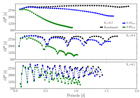
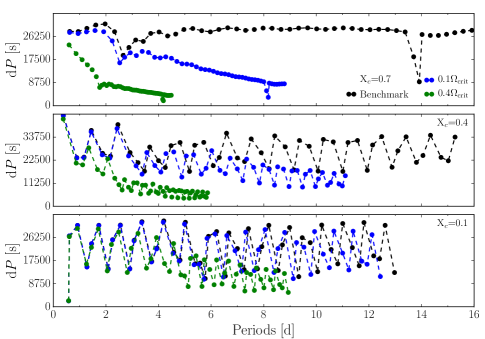
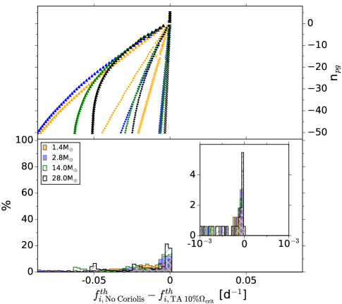
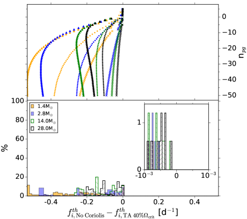
Figure 1 shows the period spacing patterns for the dipole zonal modes of the models with 1.4 M⊙ and 28 M⊙, for the three considered evolutionary stages and for the indicated rotation rate. It can be seen that rotation causes a downward tilted period spacing pattern, a property well known from theory (e.g., Bouabid et al., 2013) and also observed in Kepler data of pulsating F and B stars (e.g., Van Reeth et al., 2015; Pápics et al., 2017; Ouazzani et al., 2017). In Fig. 2 we compare the dipole zonal frequencies of modes with the same radial order , computed without the Coriolis force versus in the TA. It can be seen in Fig. 2 that the inclusion of the Coriolis force increases the gravity-mode frequencies for the entire mass range. The frequency differences increase for increasing radial order. Almost all frequency differences are larger than the typical frequency error expected for a light curve spanning about a half to one year (see Table 2). We conclude that the Coriolis force cannot be neglected in forward seismic modeling of gravity modes and that rotational effects must be included to compute theoretical gravity-mode frequencies, even for stars rotating as slowly as 10% of their critical rotation rate.
Schmid & Aerts (2016) treated two F-type super-inertial gravity-mode pulsators in a non-synchronized close binary, with near-core rotation rates of 0.09 and 0.14 d-1 and spin parameters in the near-core region () ranging from 0.14 to 0.26. They assessed that the impact of ignoring the Coriolis force on the seismically modeled isochrone age is about 5%; the radii are affected by about 3%, while the masses remain unaffected for these rotation rates. These two pulsators can hence be considered as limiting cases for the validity of ignoring the Coriolis force.
Computations of frequencies in the inertial frame of reference based on the TA require estimation of the rotation frequency, , in addition to identification of the mode degree and azimuthal order for each frequency (Van Reeth et al., 2016; Ouazzani et al., 2017). This implies that forward seismic modeling of gravity-mode frequencies is at least a 5D optimization problem, since must be estimated, along with . It was shown by Van Reeth et al. (2016) and by Ouazzani et al. (2017) that the slope of period spacing series of gravity modes of consecutive radial order in F-type pulsators allows for the simultaneous identification of the mode wavenumbers and the derivation of . This method also works for B-type pulsators (Pápics et al., 2017) and is adopted here as an essential step in our seismic modeling scheme (cf. Sect. 6).
| Comparison | 1.4 M⊙ | 2.8 M⊙ | 14 M⊙ | 28 M⊙ |
|---|---|---|---|---|
| No Coriolis TA@10% | 10% (11,9,9) | 12% (16,11,9) | 13% (22,9,9) | 17% (33,9,9) |
| No Coriolis TA@40% | 1% (2,2,0) | 3% (2,7,0) | 5% (4,7,4) | 6% (7,7,4) |
| Adiabatic Non-adiabatic | 100% (100,100,100) | 96% (93,96,100) | 83% (100,77,63) | 96% (100,91,89) |
| Ledoux Schwarzschild | 86% (67,91,100) | 80% (80,71,89) | 100% (100,100,100) | 99% (96,100,100) |
| 10% (8,6,15) | 7% (2,6,13) | 73% (55,73,91) | 81% (59,82,100) | |
| Gray Paczynski | 59% (44,42,91) | 90% (89,82,100) | 93% (89,91,100) | 97% (91,100,100) |
| Gray FASTWIND | – | – | 94% (93,94,94) | 95% (95,94,96) |
| Precomputed ZAMS From Hayashi | 7% (0,0,22) | 27% (0,2,80) | 33% (6,8,82) | 45% (20,27,82) |
| Standard network Fe, Ni added | 98% (98,96,100) | 90% (82,87,100) | 93% (89,91,100) | 100% (100,100,100) |
| OPAL OP | 41% (6,51,67) | 0% (0,0,0) | 37% (20,41,51) | 53% (26,56,74) |
| Przybilla Asplund | 2% (7,0,0) | 0% (0,0,0) | 33% (42,51,7) | 49% (56,69,22) |
| No Atomic Diffusion Settling & Levitation | – | 18% | 19% | 43% |
3.2 The adiabatic approximation
Moravveji et al. (2015) performed the first forward seismic modeling of a slowly pulsating B star. It was based on 19 detected dipole zonal modes with radial order ranging from -14 to -32 for the B8.3V star KIC 10526294 (see also Triana et al., 2015). Moravveji et al. (2015) found that the adiabatic and non-adiabatic approximations to compute the mode frequencies are equivalent for the frequency precision yielded by a nominal Kepler light curve for these gravity modes in that mass regime.
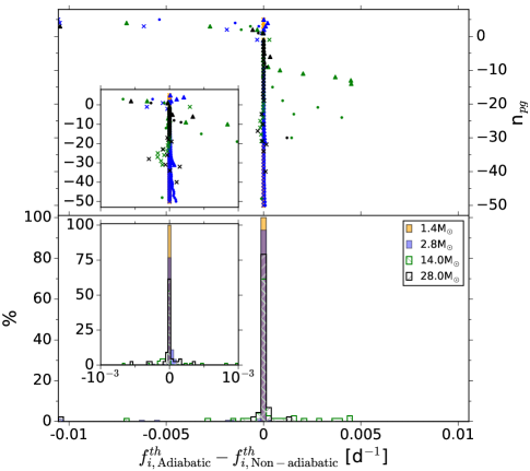
Figure 3 shows the frequency differences for the zonal dipole modes of the 12 benchmark models described in Table 1. Comparison of the range of the abscissa axes of Figs 2 and 3 reveals that the difference between adiabatic and non-adiabatic frequencies is almost always smaller than a typical frequency error for a half- to one-year uninterrupted light curve and is much smaller than the effect of rotation. Moreover, various theoretical uncertainties caused by the choice of the input physics, as discussed in the next section, give rise to much larger frequency differences.
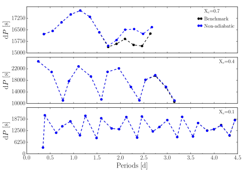
The behaviour of some modes in Fig. 3 attracts attention. It mainly concerns modes of the 14 M⊙ models and some of the 2.8 M⊙ models. We show the period spacing patterns of the converged gravity modes of the model with 14 M⊙ in Fig. 4. It can be seen that the modes at with periods above some 1.7 d have deviating non-adiabatic behaviour. These deviations between the adiabatic and non-adiabatic approximation disappear at later evolutionary stages. Similar results occur, although more sporadically, for the pressure modes of the 2.8 M⊙ model, but the deviations in frequency always remain below 0.012 d-1. Our results are in agreement with those obtained earlier by J. Daszyńska-Daszkiewicz in the framework of the HELAS project.111http://helas.astro.uni.wroc.pl/deliverables.php?active=opalmodel&lang=en Her computations revealed that the difference between adiabatic and non-adiabatic frequencies of pressure modes increases as the radial order increases and can be as large as 0.05 d-1 for or 7. Indeed, high-order pressure modes are much more sensitive to the very outer envelope of the stars, where non-adiabatic effects occur, while the gravity modes are dominantly determined by the physics of the deep stellar interior, where the adiabatic approximation is appropriate.
Our non-adiabatic computations for the excited gravity modes reveal mode lifetimes ranging from about a million years for the 1.4 M⊙ models near the ZAMS to a minimum of only 3,000 years near the TAMS. We do point out, however, that MESA does not offer a time-dependent convection treatment, so the mode excitation predictions are not optimal for this mass. We refer to Dupret et al. (2005) for more appropriate computations. The 2.8 M⊙ models reveal only a few excited modes close to the ZAMS (the case), with a relatively short liftetime of some 2,500 years. On the other hand, the 14 and 28 M⊙ models have only a few gravity modes excited near the TAMS (), with lifetimes of only some 10 years and 45 000 years, respectively. These mode excitation results are in excellent agreement with those by Szewczuk & Daszyńska-Daszkiewicz (2017), who considered models with masses between 2.5 and 19 M⊙ (these authors did not list the mode lifetimes).
The required CPU time for the computation of non-adiabatic frequencies is much larger than for adiabatic computations. Moreover, uncertain physics is involved in the non-adiabatic outer envelope of the star, while the frequencies of detected gravity modes are dominantly determined by the physical properties of the deep interior. For these reasons, we adopt the TA in the adiabatic approach in the forward modeling, because such modeling has the purpose to deduce the global physical properties of the star. However, once the forward modeling results are known, instability computations should be performed for the best models, in order to test the mode excitation and the non-adiabatic frequencies of the detected modes, as a way to improve our knowledge of opacities and assess the properties of possible missing input physics.
4 Theoretical frequency uncertainties stemming from the equilibrium models
As discussed in Sect. 3 and illustrated in Moravveji et al. (2015, 2016), the four basic parameters to be estimated from forward seismic modeling of stars born with a convective core are insufficient. Equilibrium models contain numerous additional parameters, some of which have a significant impact on the oscillation frequencies while others do not. This allows to estimate the parameters that have the largest effect on gravity-mode frequencies, after careful choice of the input physics that leaves the gravity-mode frequencies unchanged.
In order to make appropriate choices for which parameters to estimate and which to keep fixed when describing the macro- and microphysics, we need to know which processes affect the frequency values less than the resolving power of the data set. Here, we provide a hierarchy in the multitude of choices to be made among, e.g., the EOS, opacities, nuclear reaction rates, chemical mixtures, the atmosphere model as a boundary condition, the starting model at the ZAMS, etc. Whenever a different yet “fixed choice” of input physics is made without parameters to be estimated, we adopt the terminology that we are dealing with a different stellar model with free parameters and fixed physics . For each stellar model, estimation of the optimal value of its free parameters and the accompanying uncertainties of those parameters is achieved by minimizing the discrepancy between predicted from and the observations . Subsequently, stellar model selection is done by comparing the best correspondence between observed and predicted frequencies according to a well-defined criterion, for various choices of the input physics , using the optimally estimated parameters within each stellar model. This stellar model selection takes into account the number of free parameters in each stellar model and applies a penalty accordingly.
In practical applications, the difference between parameter estimation for a fixed type of stellar model , versus selection of the most appropriate input physics represented by , depends on the type of star. It is therefore essential that modelers have knowledge of the hierarchy among the parameters to be estimated versus the physical properties that can be fixed. For example, forward seismic modeling of pulsating subdwarfs or white dwarfs requires the mass of the thin outer hydrogen layer as a free parameter to be estimated along with the overall stellar mass, because it is vital to evaluate the mode trapping (e.g., Charpinet et al., 2011; Córsico et al., 2012), while rotation can be treated at the level of Ledoux splitting for such stars and does not require use of the TA (e.g. Hermes et al., 2017; Giammichele et al., 2017). Similarly, mass loss is considered not to be of importance for intermediate-mass stars during core hydrogen burning. For high-mass stars burning hydrogen in the core, modelers should make sure that ignoring mass loss or fixing it to a specified value is appropriate by considering a second stellar model, without adding the complexity of having as an extra parameter to estimate (cf. Fig. 6 below). Hence, two models , one with and one without mass loss, could be considered to check its effect on the seismic parameter estimation, relative to the measurement error of the frequencies of the detected modes. For stars beyond core-hydrogen burning, however, could be included as parameter to estimate in .
Many additional cases to those above can be discussed in the context of considering different stellar models, the choices depending on the type of star to be modeled. Below we focus on the most important ingredients to consider as different models for the specific case of core-hydrogen burning stars with a convective core, whose most important parameters for the macrophysics to be estimated will be discussed first.
4.1 Frequency errors due to choices of macrophysics
Aside from the four basic parameters needed to compute the equilibrium models during the main-sequence life of a star, , and an estimate of the near-core rotation frequency as input for the TA oscillation frequency computations, a multitude of parameters due to macrophysical phenomena are included in state-of-the-art evolution codes. We evaluate the most important ones, from the viewpoint of the uncertainty they cause in the computation of theoretical gravity-mode oscillation frequencies.
4.1.1 Convection and mixing parameters
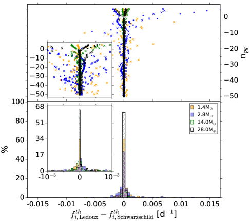
In this work, we consider stars with M⊙ at birth. The central nuclear burning for such stars is dominated by the CNO cycle, which is highly temperature sensitive. Such stars have a convective core and its mass is of major importance for the evolution of the star. For this reason, the core mass is also a dominant parameter to estimate along with . The time scale of the convection in the core is much shorter than the nuclear time scale, so we can assume full and instantaneous mixing there. Hence, the core has uniform chemical composition as long as hydrogen burning is active. We adopt the Ledoux criterion and use MESA’s predictive mixing scheme to locate the boundary of the convective core for the equilibrium models in Table 1. We show in the left panel of Fig. 5 the difference in the oscillation frequencies if we instead adopt the Schwarzschild criterion. It can be seen that igoring the -gradient in the stability criterion somewhat impacts the gravity modes for the 1.4 and 2.8 M⊙ models, and more so at evolved rather than at early evolutionary stages. The frequency differences always remain below 0.017 d-1. Paxton et al. (2018) provide a thorough discussion on the subtle differences that may occur in the inhomogeneous region beyond the core boundary due to the choice of the convection criterion, depending on the stellar mass and evolutionary stage. However, as becomes clear from Table 2, the implications for the modes due to these small differences are inferior to those of several other effects connected with choices for the input physics.
The observations of gravity-mode period spacings in a sample of F stars (e.g., Van Reeth et al., 2015) and B stars (e.g., Pápics et al., 2017) reveal detailed structure. Indeed, the period-spacing morphology appreciably deviates from a constant value, even for stars that hardly rotate (Degroote et al., 2010; Pápics et al., 2014). Estimation of the core mass from forward seismic modeling of core-hydrogen burning stars based on gravity modes was so far only done for a few stars and all of them demanded the inclusion of convective core overshooting and chemical mixing in the radiative envelope (Moravveji et al., 2015, 2016; Schmid & Aerts, 2016). Each of these two necessary ingredients are described by at least one parameter. The overall mass in the core is dependent on the treatment of the overshooting, while the chemical profiles throughout the star are determined by the element transport in the radiative envelope. We describe the physical meaning of these two required ingredients here.
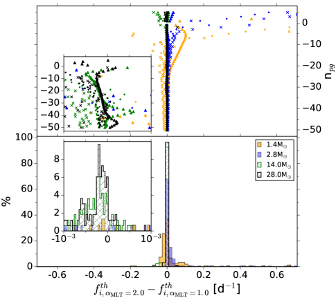
As in many stellar evolution codes, convective energy transport in MESA relies on the time-independent mixing-length theory, while time-dependent convection (turbulent pressure) is ignored. Mixing-length theory is characterized by one free parameter, , representing the characteristic length scale over which convective fluid elements travel before they dissipate; it is expressed in local pressure scale heights and takes typical values between 1 and 2. For low-mass stars, determines the convective motions in the outer convective envelope and one often fixes it to the solar value. However, the intermediate-mass stars we consider here have very thin and shallow convective envelopes. Moreover, along with the high-mass stars, they have a fully mixed convective core, where physical circumstances are very different than in Sun-like stars. For this reason, is a free parameter. We show in the right panel of Fig. 5 the effect of changing from 2.0 to 1.0. It can be seen from Fig. 5 and deduced from Table 2 that this change has major impact for the two lowest masses considered here, particularly at evolved stages. This is in line with observational results for Sct stars (Bowman & Kurtz, 2018). The choice for is less important for the two high-mass stars, particularly close to the ZAMS. The results in Fig. 5 are as expected since the two lower-mass models have shallow outer convection zones whose extent is determined by , while the high-mass stars have radiative envelopes in their early life but develop convective envelopes near the TAMS. Given the results in Table 2, one should either estimate , particularly for intermediate-mass stars, or consider at least two different fixed values to assess the impact on the forward modeling.
Complications to the above picture arise in the determination of the core boundary because convective fluid elements “overshoot” the boundary between the convective core and radiative envelope due to their inertia. The extent and properties of this overshoot region, including the level of mixing of the chemical elements inside it and its thermal structure, are of major importance for the future evolution of the star (Kippenhahn et al., 2012, Section 30.4, for a thorough discussion). Gravity modes allow us to seismically probe the detailed properties of this near-core overshoot region. The parameters describing the aspects of convective core overshooting are among the most important ones for modeling of the stars in the mass range we consider (see Sect. 3 in Paxton et al., 2018, for a thorough discussion).
In MESA, convection is implemented as a diffusive process with an associated mixing coefficient. In such a framework, the convective core has a large diffusive mixing coefficient , typically between and cm2 s-1 during core-hydrogen burning for the mass regime we consider here. As such, it is natural to describe the mixing due to core overshooting as a diffusive process as well, with coefficient containing at least one dimensionless parameter (Eq. (9) in Paxton et al., 2013). Several options are available to define the level and shape of overshoot mixing, each characterized by a set of free parameters – Paxton et al. (2013, Appendix B.7) and Pedersen et al. (2018). Among them is the option to consider an exponentially decaying prescription described by the parameter , and the simpler step function overshoot for which the core is extended into a fully mixed overshoot region from its boundary by an amount .
The temperature gradient in the overshoot region is unknown (see Salaris & Cassisi, 2017, for a thorough discussion on chemical mixing and temperature gradients). In the standard version of MESA, it is the radiative gradient but the code is sufficiently flexible to change this into the adiabatic one (so-called convective penetration) or any transition between these two. These choices each constitute a different stellar model . In regions where the temperature gradient takes a value between the adiabatic one and the adiabatic one increased with a positive gradient, semiconvective mixing occurs. This phenomenon describes the growing oscillatory motion of a convective fluid element in that region, which implies partial chemical mixing in that zone. The effect of semiconvection on the temperature gradient is unknown. In MESA, semiconvective mixing in the vibrationally unstable region is again implemented as a diffusive process, characterized by the dimensionless coefficient . The larger the coefficient, the faster the matter mixes in the semiconvective zone.222In this work, we ignore thermohaline mixing (“fingering convection”) due to a negative -gradient value in the models. This phenomenon of slow mixing typically occurs in evolved low-mass stars with shell burning. It can also occur during the hydrogen core burning but the mixing profile it would cause is not well known (Deal et al., 2017). Should a profile become available, this phenomenon could be included separately with yet another diffusive coefficient , and could easily be included in our statistical formalism.
As already discussed above, “extra” macroscopic mixing occurs in the zone above the core overshoot zone in the radiative envelope of intermediate-mass and high-mass stars. Indeed, such extra mixing was required to bring theoretical frequencies in agreement with observational data (Moravveji et al., 2015, 2016). Coherent oscillation modes (Aerts et al., 2014) and damped modes (Rogers & McElwaine, 2017) may also induce mixing but these options have so far hardly been taken into account in stellar evolution theory. In order not to introduce bias on the importance of the various phenomena giving rise to element transport, we take a pragmatic approach and make use of one diffusive mixing coefficient as free parameter in the forward seismic modeling. This parameter represents the average overall effect of (rotationally and/or magnetically and/or pulsationally induced) mixing in the radiative zones of a star as probed by the gravity modes. Only if this free parameter can be estimated with good precision from seismic data for a considerable sample of stars can we start to unravel the role of the various individual causes of mixing at play in the stellar envelope. As said, the first steps in this direction were taken for a few stars (Moravveji et al., 2015, 2016; Schmid & Aerts, 2016), which showed the need to include just adjacent to the core overshoot region in the radiative envelope to explain the structure in the observed period spacings. Meanwhile, Pedersen et al. (2018) assessed if gravity modes can distinguish between a constant versus an actual profile stemming from 2D simulations of internal gravity waves. These authors found that a distinction can only be made on the basis of combined observational restrictions from gravity modes and surface abundances. In first instance, it is therefore justified to consider to be a single parameter, describing the mixing adjacent to the core overshoot zone to be estimated.
As a side remark, we point out that extra turbulent mixing in the surface layers of intermediate-mass stars is sometimes also considered in the context of asteroseismology or galactic archeology. Such extra turbulent mixing in the near-surface layers is usually assumed to have a density dependence. Aside from this, envelope undershooting may also occur. While both these phenomena are important for chemical tagging at advanced evolutionary stages of low-mass stars (e.g., Dotter et al., 2017), they hardly affect the gravity mode period spacings (Pedersen et al., 2018). Indeed, mixing in the zone adjacent to the core-overshoot zone is much more important for the fitting of detected gravity-mode frequencies, because these modes mainly probe the near-core regions. At first instance, such surface mixing can therefore be ignored in forward seismic modeling of gravity modes but can be evaluated from high-precision surface abundances if available.
The transport of angular momentum during a star’s evolution is also not calibrated by observations, just as the element transport. Moreover, the level of its inhibition by -gradients is not known. Even for the simple case of low-mass stars born with a radiative core, where the macroscopic mixing is thought to be absent, current theory of angular momentum transport fails (e.g., Eggenberger et al., 2017). The importance of a convective core and near-core properties during core hydrogen burning for appropriate understanding and interpretation of angular momentum of red giants was recently highlighted (Tayar & Pinsonneault, 2013; Eggenberger et al., 2017). Seismic modeling of intermediate-mass stars from gravity modes during the core hydrogen burning is highly relevant to understand the angular momentum of secondary clump red giants as well as more massive blue supergiants.
Given the major uncertainties in the transport of chemicals and angular momentum in current stellar evolution theory, an appropriate approach in terms of forward seismic modeling is to estimate the chemical mixing by seismic inference from gravity modes, assuming rigid rotation near the core as first step (cf. Van Reeth et al., 2016; Aerts et al., 2017; Ouazzani et al., 2017). Subsequently, the rotation profile and the accompanying angular momentum transport can be evaluated by considering instead of constant for the best seismic models, once their mixing properties have been derived seismically. This approach has been applied to the above mentioned 3.25 M⊙ star KIC 10526294 by Moravveji et al. (2015) and Triana et al. (2015), pointing to the need of angular momentum transport. The required transport could meanwhile be explained by internal gravity waves (Rogers, 2015). Such type of analyses needs to be done for stars with various levels of near-core rotation to deduce a broad range of covering the entire hydrogen-burning phase, in order to be able to predict angular momentum transport for the more evolved phases (Aerts et al., 2017; Ouazzani et al., 2018).
In summary, near-core rotation, convective core overshooting and mixing in the radiative envelope adjacent to the core overshoot zone must all be included in the forward seismic modeling of gravity-mode pulsators with M⊙, implying that the optimization problem is at least 7-dimensional (+7D), with . For intermediate-mass stars, one should additionally test the impact of a different mixing length value.
4.1.2 Choice of a static atmosphere as boundary condition
All stars experience mass loss during their life. The occurrence and duration of the episodes of mass loss are vastly different for stars with different masses. Low- and intermediate-mass stars born with M⊙ experience substantial mass loss due to a dust-driven wind on the asymptotic giant branch, while more massive stars experience a radiation-driven wind during and/or beyond core hydrogen burning until they explode as supernovae. Two important parameters characterizing the wind are the mass-loss rate and the wind velocity profile (Kudritzki & Puls, 2000).
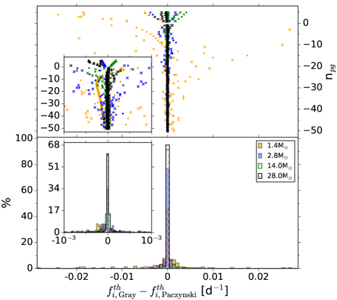
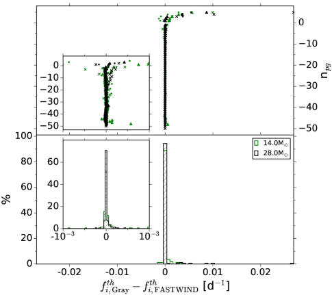
Stellar evolution computations treat the stellar wind in a simplistic way in the sense that a mass-loss rate from a recipe is adopted and the appropriate mass is peeled off the outer layers of a star at each time step in the evolution, taking into account the accompanying angular momentum loss and assuming that hydrostatic equilibrium holds at every time step. This is a crude approximation, because the driving force of the wind is ignored in the equation of motion and a static rather than dynamical atmosphere is considered as boundary condition to solve the equations of stellar structure. MESA and GYRE offer various static atmosphere models from precomputed tables as choices for these boundary conditions. The effect of different choices of the atmosphere model on the frequency values of gravity mode is illustrated in the left panel of Fig. 6, where we show the frequency differences obtained for a gray versus Paczynski atmosphere model. It can be seen that frequencies are only modestly affected and that the majority of frequency differences are within the resolving power of a typical data set, except for the lowest considered mass M⊙ at evolved stages. The latter models have a thin convective outer envelope and the interplay amongst convection, pulsation, and atmospheric properties becomes important for the modes. For stars without a (thin) convective outer envelope, the range of the frequency differences is always below 0.01 d-1 (Fig. 6), which justifies that we neglect this effect compared to other more important ones.
4.1.3 Effect of mass loss due to a radiation-driven wind
So far, the mass-loss rate was not considered as a parameter to estimate in forward seismic modeling for core-hydrogen burning stars, given that one is already dealing with a +7D optimization problem. Cluster ensemble asteroseismology from Kepler low-mass red giants did allow a rough evaluation of the upper limit of mass-loss rate due to a dust-driven wind on the red giant branch (Miglio et al., 2012). However, the potential to estimate seismically and take into account angular momentum loss during stellar evolution is appealing in view of the core rotation rates found for intermediate-mass stars (Aerts et al., 2017).
We test here how the parameter affects the gravity-mode frequency predictions. As shown in the left panel of Fig. 6, forward seismic modeling of gravity modes is not affected by the choice of the atmosphere in the case of static models to compute the boundary conditions, because such modes are determined by the properties of the deep stellar interior. Nevertheless, the mode cavities are affected by the interplay between the stellar wind and for a dynamical atmosphere, energy wave leakage and angular momentum loss are predicted to occur (Townsend, 2000a, b). We considered a simplified test by comparing the difference in adiabatic gravity-mode frequencies for a static gray atmosphere versus a dynamical atmosphere for particular values of the mass-loss rate as indicated in Table 1. For each of the parameters of those benchmark models in Table 1, we took the outcome of the MESA model for the luminosity, radius, and effective temperature in the case of a gray atmosphere. Along with the mass and mass-loss rate, these values were then used for the calculation of a radiation-driven stellar wind structure with the NLTE radiative transfer code FASTWIND (Puls et al., 2005). In this code the wind structure is derived from the mass continuity equation and a pre-described velocity field derived from standard radiation line-driven wind theory, , with the stellar radius and the terminal wind speed as given by MESA. NLTE Hopf functions are used for the temperature stratification using an exact relation from a converged plane-parallel NLTE model (with the Rosseland optical depth) and taking into account sphericity effects (see Santolaya-Rey et al., 1997, for an extensive description). This atmosphere and wind structure was then stitched to the interior structure from MESA. The point of connection was chosen as the one where the opacities of both models match best at . A smooth and continuous connection was enforced by linear interpolation of the various quantities in log space around the point of connection.
The comparison between the frequencies of the modes for a static gray atmosphere versus a dynamical FASTWIND atmosphere is shown in the right panel of Fig. 6 for the highest two considered masses (for the lower masses, computations with FASTWIND are not meaningful). We find it justified to ignore the wind for gravity modes, but not for pressure modes. However, we note that our simple test here only accounts for the wind outflow indirectly through a modified atmospheric structure, i.e., we do not explicitly account for potential wave leakage when solving the pulsation equations within GYRE. As such, the effects seen in Fig. 6 quite likely constitute lower limits.
Any radiation-driven wind effect was so far ignored in seismic modeling of Cep stars based on ground-based data. Given that stars born with a mass above some 24 experience strong mass loss throughout their entire life and stars with as of the blue supergiant phase, should be considered as an additional parameter to estimate from forward seismic modeling of such stars. Unfortunately, seismic data sets to achieve this are currently not yet available for stars with mass above some 24 M⊙. Major progress on this front is within reach of the TESS Continuous Viewing Zones (Ricker et al., 2016) and the long pointings of the PLATO mission (Rauer et al., 2014).
4.1.4 Treatment of the pre-main sequence evolution
Solving the stellar structure equations not only requires boundary conditions at the centre and the surface of the star, but also initial conditions. In essence, an initial “birth model” is required to “start” the evolution from core-hydrogen burning in full equilibrium and the age of the star is determined as of that so-called Zero Age Main-Sequence (ZAMS) model. However, partial nuclear burning already occurs during the contraction phase of the protostar, so there is no one-to-one equivalence between the stellar age and at the ZAMS. Moreover, the physical processes during star formation, including rotation, magnetism, and accretion during contraction from the Hayashi track towards the start of core hydrogen burning in equilibrium at the ZAMS, remain largely unknown. In view of this, one tends to circumvent pre-main-sequence evolutionary computations. MESA comes with a library of pre-computed ZAMS models for and with masses between 0.08 and 100 M⊙ (Paxton et al., 2011). An option to start the evolutionary computations offered to users is to interpolate between these pre-computed ZAMS models, in order to achieve a ZAMS model for the chosen mass. We have tested this procedure against the more time-consuming computation of contraction models for the chosen from the Hayashi track to the ZAMS to end up with a self-consistent ZAMS model according to the chosen and frozen input physics as initial conditions.
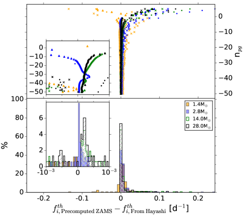
Comparing the frequencies between those two cases is non-trivial as one in fact evolves two slightly different stars as of the ZAMS. For this comparison, Fig. 7 shows the difference in the oscillation frequencies of models at equal values of to within 0.001. This figure demonstrates that taking an interpolated ZAMS model from MESA’s pre-computed libraries versus a ZAMS model resulting from contraction starting on the Hayashi track with consistent input physics for the chosen changes the frequencies more than the typical frequency error derived from a half- to one-year light curve for the majority of modes. It is therefore essential to compute models from the Hayashi track to end up with proper initial conditions in forward seismic modeling.
Unlike the interior rotation, core overshooting and envelope mixing, we cannot treat the “global characteristics” of the ZAMS model as a simple free parameter to estimate during the seismic modeling. This aspect is rather a typical case where various choices for the input physics during the pre-main-sequence phase each constitute a different stellar model . The dependence of the frequency values on the pre-main-sequence structure is good news for future forward seismic modeling of pre-main-sequence pulsators. While applications of seismic modeling to this early phase of stellar evolution must await suitable photometry from space, the same methodology than described here can be used for these early evolutionary stages once sufficiently identified modes can be measured (e.g., Zwintz et al., 2014, 2017).
4.2 Errors due to choices of microphysics
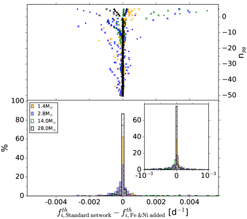
Aside from the aspects of the macrophysics discussed above, a myriad of choices for the microphysics can also be made to compute the stellar models. It concerns, e.g., the Equation-of-State (EOS), thermonuclear and weak reactions, nuclear reaction networks, opacities, etc. Here, we focus on the core-hydrogen burning phase for stars that do not undergo electron degeneracy. Such cases are the best understood ones in terms of the EOS (an ideal gas with radiation is appropriate). Moreover, the choices of the nuclear reactions and of the nuclear reaction networks among a variety of sets affect the seismic properties least during this simplest evolutionary phase, but may appreciably alter the more advanced phases of stellar evolution. For this work, we used the standard MESA EOS, the NACRE rates (Angulo et al., 1999) and the MESA basic rate network based on eight isotopes: 1H, 3He, 4He, 12C, 14N, 16O, 20Ne, and 24Mg (Paxton et al., 2011). As an illustration of the effect of such a choice, we also computed the oscillation frequencies in the case where the 56Fe and 58Ni isotopes were added to the network and provide the comparison in Table 2 and Fig. 8. It can be seen that, as expected, this only has a minor effect compared to other aspects of changing the input physics.
We now turn our attention to some of the more critical aspects of the microphysics that affect the oscillation frequencies appreciably.
4.2.1 Opacities and chemical mixtures
It is well known that the choice of opacities affects the oscillation properties of B-type pulsators appreciably (e.g. Daszyńska-Daszkiewicz & Walczak, 2010). In their extensive study of KIC 10526294, Moravveji et al. (2015) quantified the effect of choosing different opacity tables and mixtures for the equilibrium models on the resulting frequency predictions for gravity modes (see their Fig. 3). Two different sets of opacities – OPAL and OP – were combined with three different chemical mixtures to end up with six different models , adopting the MESA EOS. The six corresponding dipole zonal frequencies for the mode with radial order differ up to d-1, while the frequency differences for the mode with radial order amount to d-1. This already demonstrated that the theoretical frequency uncertainty due to different choices of opacity tables cannot be ignored.
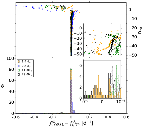
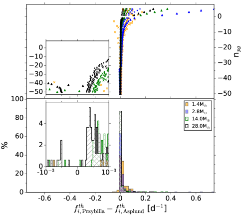
Figure 9 shows the deviations between the theoretical frequencies for the benchmark models in Table 1 due to a different choice of opacities (left) and chemical mixture (right). Both these choices have a major effect on the frequency values in the sense that the differences are larger than the frequency error of a typical half- to one-year light curve. Both the pressure-mode and gravity-mode frequencies get shifted with a systematic effect that cannot be ignored. We conclude that, with the current poor knowledge of opacities, asteroseismology in the mass regime considered here should be based on various stellar models relying on different opacity tables and chemical mixtures.
4.2.2 Microscopic atomic diffusion
In addition to the aforementioned parameter to be estimated in the radiative envelope, composition changes may also occur due to transport processes following microscopic atomic diffusion in the radiative layers of the star. The computation of such microscopic processes requires detailed evaluation of frequency-dependent absorption coefficients and re-evaluation of opacities from all the relevant ions involved in the various layers of the star, for each time step along the evolution. This obviously constitutes an immense challenge for the evolutionary computations (CPU-wise) and is usually omitted for massive stars as these evolve on a timescale of millions of years. For cool stars with an extensive convective envelope, it is necessary to consider models with gravitational settling for evolutionary computations (e.g., Michaud et al., 2004) and for proper chemical tagging for galactic archeology (Dotter et al., 2017). Here, we investigate the effect of atomic diffusion for intermediate- and high-mass stars, which also requires the inclusion of radiative levitation (e.g. Deal et al., 2016, 2017).
Within MESA, four components of atomic diffusion can be included, each for various chemical elements: gravitational settling, concentration diffusion, thermal diffusion, and radiative levitation (Hu et al., 2011; Paxton et al., 2015). Including atomic diffusion in MESA requires any of these phenomena to be turned “on” or “off”, i.e., the activation of any of these particular microscopic effects can be included or not. Moreover, each of the phenomena can be included with or without a parameter to be estimated. In our methodological set up, including atomic diffusion for each different chemical element would imply for each a different stellar model . For low-mass stars (e.g., Verma et al., 2017) and for white dwarfs (e.g., Romero et al., 2017), gravitational settling is an important ingredient for asteroseismic modeling. On the other hand, radiative levitation acting upon Fe and Ni is critical to take into account when estimating oscillation frequencies for hot subdwarfs in core helium burning (e.g., Charpinet et al., 2011; Bloemen et al., 2014).
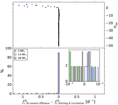
For the stars under study here, we show in Fig. 10 the comparison between the frequencies due to models without and with atomic diffusion. For this comparison, we used the treatment by Hu et al. (2011), as implemented in MESA, taking into account gravitational settling, concentration diffusion, thermal diffusion, and radiative levitation for the elements H, He, C, N, O, Ne, Mg, Fe and Ni. For this comparison we limited to the models from the ZAMS until for CPU reasons, where we adopted the most recent MESA implementation (Paxton et al., 2018). In this comparison, we omit the models with M⊙, because settling is the dominant effect for those and this requires some level of turbulent mixing (combined or not with envelope undershooting) to be included in the model computations, in order to end up with appropriate surface abundances of metals (see, e.g., Turcotte et al., 1998, for pioneering work). One usually takes such ad-hoc turbulent mixing to be a function of density (e.g., Richer et al., 2000; Deal et al., 2016; Dotter et al., 2017). Since our baseline models do not have such density-dependent turbulence, nor undershooting, the comparison with the baseline models indicated in Table 2 is not meaningful for this mass.
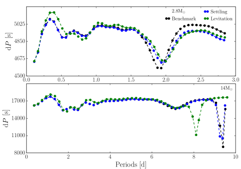
Figure 10 and Table 2 reveal that atomic diffusion has a large effect on the frequencies for all the modes. We find that this is mainly due to the radiative levitation for the three masses we considered here. This is illustrated for the period spacing patterns of the 2.8 and 14 M⊙ models in Fig. 11, where it is seen that the mode trapping changes when radiative levitation is taken into account, because it modifies the -gradients and hence the convection zones. The importance of radiative levitation was already stressed by Deal et al. (2017) in their study of the solar-like oscillations of the F-type exoplanet host star 94 Ceti. Radiative levitation has so far hardly been included in forward seismic modeling of gravity modes, mainly because it is too demanding in computation time. Our results show it to be worthwhile to undertake future studies on how to include the combined effect of settling and levitation in the forward modeling of intermediate-mass and high-mass stars.
As a side remark in this section, we stress that atomic diffusion may be of importance locally in and near the driving layer in the envelope for mode excitation of opacity-driven modes during the main sequence, since more modes are detected than predicted to be excited in massive stars (e.g., Moravveji et al., 2016; Daszyńska-Daszkiewicz et al., 2017). For this reason, mode excitation is not part of our forward seismic modeling scheme but is treated as a posteriori evaluation of how good the best seismic models are in terms of explaining overall stellar properties, along with other observables such as a spectroscopic and , surface abundances, and luminosities deduced from Gaia astrometry.
In general, our statistical framework outlined in the following sections is only based on gravity-mode frequencies and does not rely on surface properties from spectroscopy, nor on astrometry or interferometry. The reason is that the gravity modes provide direct observational information on the deep stellar interior, at the level of , while the relative precisions for , and abundances from spectroscopy of stars in the mass range considered here are far worse, often above 10% (e.g. Morel et al., 2008; Martins et al., 2012b, a; Van Reeth et al., 2015). Moreover, our aim is to tune the near-core interior properties of the stars. After deducing the best seismic models, we will confront their predictions with measured surface properties, to assess the physical conditions in the outer envelopes of the stars. In this respect, our set-up and application is quite different than the case of low-mass stars with pressure modes. Of course, whenever additional spectroscopic, interferometric or astrometric data would become available at precise enough level for our scientific aims, it can also be used as input in the forward modeling, together with the oscillation modes. Currently, this is not yet the case for the mass regime we treat here.
5 Statistical model formulation and parameter estimation
We now place the principles outlined in the previous Sections 2, 3, and 4 into a formal and appropriate statistical framework. We assume that we have various stellar model grids based on different stellar models , along with their pulsational frequencies, at our disposal. We want to reach two major goals:
-
1.
to fit as closely as possible the observed and identified gravity-mode oscillation frequencies () by model (theoretical) values . As outlined above, we are in the situation that some of the uncertainties on the theoretical frequencies are smaller than the errors of the observed frequencies, while others are larger or of the same order of magnitude. The overall theoretical errors (for ) are unknown, because additional factors than those shown in Figs 2 – 10 are at play, such as the limitation to 1D stellar structure models, the absence of certain forces, missing input physics, etc. Hence, heteroscedasticity must be included in the statistical model formulation.
-
2.
to select the most likely physical model for a single star or for an ensemble of stars, without introducing a priori bias about the unknown input physics, and in particular keeping in mind that we are dealing with a different physical regime compared to Sun-like stars with a radiative core: here, the Coriolis force, core overshooting and transport of elements in the radiative envelope are dominant phenomena that cannot be ignored.
This setting is different from many statistical problems of parameter estimation, where a single parameter vector is estimated from a set of repetitions. Here, we are not dealing with replicates of one and the same mode frequency but rather with a single measurement for a set of observed frequencies () belonging to modes that each have their own mode cavity and probing power for the interior physics. Each of the measurements, , is accompanied by its own single error measurement for which we assume .
We now introduce convenient vectorial notations to outline the above aims into suitable statistical frameworks. An observation takes the form of a vector , consisting of the observed frequency values, with , where the length of the vector, , is star specific (the number of identified gravity modes). Let us denote the measured frequency precisions as , a diagonal matrix with elements . Given a physical model , a vector of stellar parameters, and a vector of fixed properties that is assumed known, the model predicts the observation: , where is a vector of predicted frequencies from model for the identified frequencies corresponding with . Denote by the length of vector . For convenience, will sometimes be dropped from notation: . The inclusion of a parameter in the statistical model allows to separate key parameters to be optimized (grouped in ) from the ones that are considered fixed for the fit. This is necessary when the overall parameter vector (grouping and ) is high-dimensional as in our problem of forward seismic modeling.
In our application, the number of detected gravity modes with well-determined frequency, , is typically between 10 and 40 when dealing with nominal Kepler data but smaller for other data sets, while is at least seven: aside from the four standard input parameters for the computation of stellar evolution, , we need to estimate as well the near-core rotation with period , at least one parameter connected with the core overshooting, , and one parameter describing the mixing in the radiative envelope responsible for the mode trapping. Ideally, however, is larger, as one also wants to estimate the profiles of the core overshoot, envelope mixing, and interior rotation. As a concrete example of this approach in the literature, was taken to be (hence ), while stood for fixed values of , , , along with the fixed choices of the MESA EOS, the chemical mixture by Przybilla et al. (2013), and OPAL opacities, in “Model 4” of the study of the ultra-slow rotator KIC 10526294 by Moravveji et al. (2015). The latter authors tested the performance of this Model 4 with respect to a simpler stellar model having no extra diffusive mixing in the envelope, i.e., a stellar model with () and defined by , , , with the same fixed choices of the MESA EOS, chemical mixture, and opacities (“Model 1” in Moravveji et al., 2015). The result was that Model 4 gave a better representation of the detected zonal dipole gravity mode frequencies than Model 1, hence the conclusion that this star undergoes envelope mixing in addition to core overshooting. In such an experiment, Models 1 and 4 are called nested models, because Model 4 has one more parameter to estimate than Model 1 but is otherwise the same.
Commonly, the estimation of is evaluated in all points of a grid. This grid can result from a cartesian product in the components of , but this is not a necessary requirement. Also, in practical applications, the grid will be finer in one component than in another. Let us index the grid points by a single index . This leads to a collection of theoretically-generated vectors in each grid point , denoted as . These vectors each have length . They result from the theoretical model that lies at the basis of the grid. We consider and distinguish between the following four problems to solve:
- Problem 1
-
Given one set of observed identified frequencies and a theoretical model used to compute a grid with grid points, find the most plausible value for from the grid, i.e., select for which comes closest to . By extension, a small set of candidate can be selected. Assess the errors of the selected .
- Problem 2
-
We wish to compare the capacity of various theoretical models to describe the data. In order to tackle this, it is convenient to compare the estimates among two theoretical models, and . The problem is thus for a given value of the vector from a benchmark model of grid , to find candidates from grid that provide the best match.
- Problem 3
-
Search for a statistical model to replace theoretical model , delivering an outcome vector sufficiently close to but much faster to evaluate and lending itself for error estimation of and for statistical model selection.
- Problem 4
-
Find the most adequate theory , among a collection of competing theories, using a set of stars with (where .
We provide methodology to treat each of these four problems in the following subsections, adopting vectorial notation as is common in statistics.
5.1 Problem 1: A Mahalanobis distance based solution to match the identified gravity modes of one star
The problem is to find the value for that best predicts the stellar observation , say, with corresponding value . We need to select such that the distance between and is smallest, keeping in mind the measured frequency precisions . One should accommodate two features. The first is that the variability in one component of may be larger than in another; in addition, the units may vary from component to component. This implies that standardization is necessary. The second feature is that correlations occur between the components of (cf. Fig. 5 in Moravveji et al., 2015; Pedersen et al., 2018). The stronger a component correlates with the other components, the less independent information it contributes. An appropriate solution to this problem is offered by the Mahalanobis distance (Johnson & Wichern, 2002):
| (1) |
where , the variance-covariance matrix of the vector . The Mahalanobis distance naturally takes into account correlations among the components of and reduces to the Euclidean distance in absence of any such correlations, i.e., when is a diagonal matrix.
To evaluate Eq. (1), we need an expression for . This matrix can be seen as the intrinsic variability in across a relevant range of . The grid based on , especially when sufficiently fine, will provide an approximation of this quantity when computed over a reasonable range of . This implies that it can be estimated from the grid. Considering all grid points gives:
| (2) |
where the average is
In practice, we will typically evaluate Eq. (1) using all grid points:
| (3) |
Taking the measurement errors of the frequencies into account in the computation of the Mahalanobis distance is done by replacing by in Eq. (3). Note that the inverse may need to be replaced with the Moore-Penrose inverse (Penrose, 1955) for models that are not of full rank (see the statistical models treated in Problem 3). Expression (3) provides a more appropriate measure than the often used based on an Euclidian distance, which does not take into account the correlated nature of the components of the vector .
As for a first estimate of the error of , we consider the Mahalanobis distance to comply with a normal distribution. In that case, it follows a distribution. Let the critical point be , i.e., . We then consider the empirical prediction ellipsoid across a relevant part of the grid:
| (4) |
The theoretical ellipsoid would range over all in continuous space, which is impractical, of course. As a consequence, the prediction ellipsoid depends on the coarseness of the grid, so it is essential to have it sufficiently fine yet covering an approriately broad range for . We can circumvent this below when treating Problem 3, where is determined from a statistical model rather than a theoretical model. In the case that this can be done successfully, we improve the error estimation from Eq. (4) by relying on the errors of the parameters of the statistical model to determine the errors of .
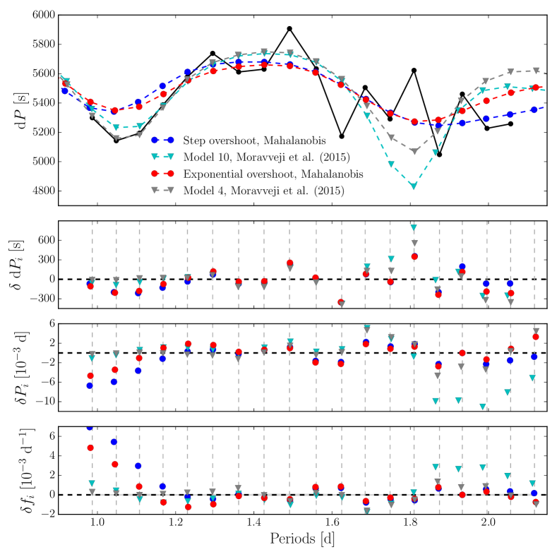
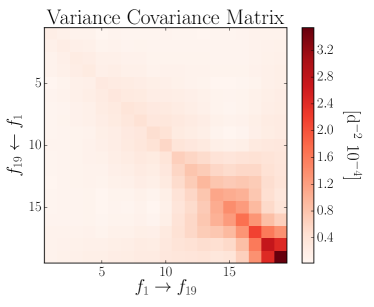
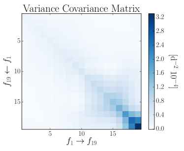
| Statistic | (cm2 s-1) | ||||
|---|---|---|---|---|---|
| 3.25 | 0.014 | 0.627 | 56.2 | ||
| 3.24 | 0.017 | 0.644 | 177.8 | ||
| 3.19 | 0.019 | 0.628 | 56.2 | ||
| 3.23 | 0.017 | 0.640 | 177.8 |
As an illustration of the benefit of with respect to a statistic, we rely on two very dense seismic model grids computed to explain the 19 identified dipole zonal modes of the slowly pulsating B star KIC 10526294 by Moravveji et al. (see Table 1 in 2015, for the frequencies and Table 3 for the grids and selection of the best models 4 and 10 from a statistic). Both these grids have and their input physics only differs in the treatment of the core overshooting, with one grid using exponential overshoot described by the parameter and the other grid relying on a step overshoot with parameter (both have the radiative temperature gradient in the overshoot zone). This star rotates at less than 1% and it revealed zonal modes with unambiguous identification from rotational splitting, so rotation can be ignored for the matching of the mode frequencies.
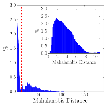
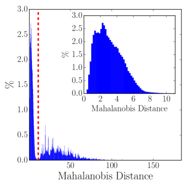
With our description based on the Mahalanobis distance in Eq. (3), we improve the modeling compared to (Moravveji et al., 2015) by taking into account the correlations among the parameters , as well as allow non-linear dependence of the observed frequencies on those five parameters. The parameter estimation from the two grids based on and are listed in Table 3. The period spacing patterns of the best solutions are compared with the observed ones in Fig. 12, while the two variance-covariance matrices for the two grids, (hence taking into account the measured frequency errors) are shown in Fig. 13. The observational errors decrease from 0.000057 d-1 for d-1 to 0.000036 d-1 for d-1. Hence, almost all the variance represented in Fig. 13 comes from the variability in the model grid predictions of the frequencies.
It is found that the estimated parameter values for are not exactly the same, yet very similar in value. The selection by Moravveji et al. (2015) focused on the best agreement for the lowest-order modes, while the Mahalanobis distance selects models that give the overall best agreement. From the middle two panels of the figure, we deduce that the largest discrepancies between observed and theoretically predicted modes for the prediction occur for the highest-order modes and reach to about 900 s, while the Mahalanobis prediction has the poorest agreement for the lowest-order modes at a level of about 600 s. All differences between the frequencies of the four considered models and KIC 10526294 translate into . Moreover, the discrepancy between the model and observed frequencies in the bottom panel of Fig. 12 are smaller than most of the theoretical uncertainties found in Sections 3 and 4 (see upper left insets of Figs 2 – 10). Hence, with the current knowledge of stellar interiors, this is an excellent overall agreement (we have stretched the ordinate axes in Fig. 12 for optimal visibility of the small discrepancies).
Given that these two dense grids resulted from a zoom-in based on an initial screening of a much sparser one, optimally tuned to comply with the data, we expect the error estimation according to Eq. (4) to encapsulate these entire dense grids. Their ranges are given in Table 2 of Moravveji et al. (2015, Mixing Grid & Step Overshoot Grid) and the distribution of the Mahalanobis distances is shown in Fig. 14. The dashed vertical line is the cutoff value. About half of the models in the two grids have a lower distance and as expected, the two prediction ellipsoids for span the entire grids in both cases. As a final note, we point out that the best models selected by the Mahalanobis distance do not change the inversion results for the rotation profile of the star determined in Triana et al. (2015). Indeed, it was already shown in that paper that this profile was hardly dependent on the best forward model selection as long as it provided a reasonable match to the zonal mode frequencies.
5.2 Problem 2: A Mahalanobis distance based solution to compare two stellar models
A pertinent question in seismic modeling of stars with a convective core is whether the core overshooting is better described either by a step function or by an exponentially decaying one. Pedersen et al. (2018) assessed the capacity of the nominal Kepler data to achieve such a comparison based on gravity modes. Another case of comparing the capacity of two stellar models was already mentioned above, namely with and without chemical transport in the radiative envelope (Moravveji et al., 2015; Pedersen et al., 2018). Such assessments require comparison between two theoretical models, and . We assume, of course, that both models produce observation vectors and , respectively, of the same length and having the same meaning for all of their components. That said, the length of the vector and the meaning of the components of and may be different.
A Mahalanobis-based solution, similar to that of Problem 1, is considered. It should be clear that there is some asymmetry to the problem, as each of the two grids has its own metric. Denote the grids by:
-
•
For , we have resulting grid points , with ;
-
•
For , we have resulting grid points , with .
Let the variance-covariance matrix , like in Eq. (2) correspond to the first grid, with the equivalent quantity corresponding to the second grid. Suppose that a benchmark model computed from the first theory with parameters results in frequencies , then we need to find
| (5) |
In the other direction, we pick a benchmark model computed from the second theory with parameters resulting in frequencies , and we need to we solve:
| (6) |
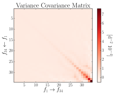
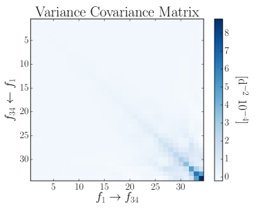
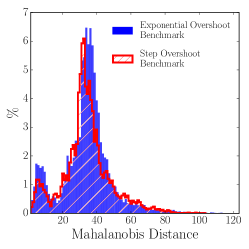
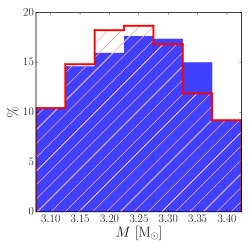
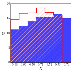
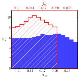
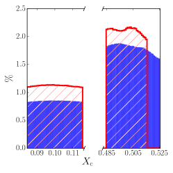
As an illustration of this Problem 2, we rely on the 4D grids of stellar models computed by Pedersen et al. (2018, Table 2) and their high-order dipole modes with periods ranging from 0.8 to 3 d. For computational reasons, these grids were centered around two evolutionary stages ( near 0.5 and 0.1). We consider the frequencies of the dipole prograde gravity modes as to be those of the benchmark model from the step overshoot grid with = and we search for the best model in the grid computed for exponential overshooting with instead of to ascertain which of the exponential overshoot models explains the one with the step overshooting of the benchmark model best. We refer to Pedersen et al. (2018) for the details on the fixed input physics , which is the same for both grids except for the mixing efficiency in the overshoot region.
We show the variance-covariance matrix in the left panel of Fig. 15, revealing once again that the dominant variability among the models in the grid occurs for modes in the high-frequency domain. The Mahalanobis distance leads to the parameters estimation given by == from Eq. (5). The distribution of the best solutions for the parameters are shown, along with the Mahalanobis distance distribution, in Fig. 16 (red). The parameter distributions were constructed by giving every grid point a weight according to the minimum Mahalanobis distance of the entire grid divided by the Mahalanobis distance at this grid point .
Conversely, we select the dipole prograde gravity-mode frequencies from a benchmark model with exponential overshoot == and we search for the best model in the grid computed for step overshooting with parameter to find == from Eq. (6) as represented in Fig. 16 (blue), with the variance-covariance matrix given in the right panel of Fig. 15. It is visually clear that this problem set is asymmetric, as demonstrated by the asymmetry of the distributions of the parameters (red) and (blue). This reflects the fact that the parameters and correlate differently with . Such a different correlation structure was also hinted at from modeling of close binary companions with a convective core (Claret & Torres, 2017) but was not yet taken up coherently in treating determinations of core masses in such objects from isochrone fitting. The bottom right panel of Fig. 16 shows the power of the Mahalanobis distance to perform stellar aging from gravity modes as there is no confusion between young and old models. Finally, the mass and initial hydrogen distributions in Fig. 16 show the opportunity to determine stellar masses with high precision from gravity modes, typically better than 5%, while the chemical composition is harder to derive as it suffers more from the degeneracies among the parameters.
5.3 Problem 3: Fitting a statistical model to frequencies generated from a physical model
Given that evaluating theoretical models and their frequencies is computationally expensive, one might aim to replace the derived from a theoretical model in the grid points with a statistical model, sufficiently close in outcome but easier to evaluate. Such a situation typically occurs when grids of stellar evolution and pulsation computations turn out to be insufficiently fine for forward seismic modeling and one wants to avoid having to re-compute models with a too extensive number of extra grid points (cf., Moravveji et al., 2016). Therefore, we write such a statistical model as:
| (7) |
In other words, we treat the vectors with frequencies resulting from a theoretical model as outcome variables and we want to describe these outcome variables by a function . The latter can be linear or non-linear. The statistical model will typically contain unknown parameters to be estimated, grouped in a vector . Because a perfect match between the frequencies resulting from the theoretical stellar model and from the statistical approximate model never occurs, we introduce an error term for each grid point, , with variance-covariance matrix . Hence, we rewrite the statistical model (7) as:
| (8) |
where is the error of the estimated frequency vector in the grid point resulting from the statistical model. At the level of the individual frequencies labeled with , Eq. (8) can be written as:
| (9) |
with , the th diagonal element of . Also, , the covariance, and the off-diagonal element of .333 Note that we use the notation for the generic element of a variance-covariance matrix , as is commonly done in the statistical literature. The elements correspond to variances if and to covariances if (Johnson & Wichern, 2000). The corresponding standard deviations are then . So, in general, each regression component is allowed its own variance for , implying heteroscedasticity, as required following Sections 3 and 4.
With this setup, we assume that the normal distribution offers a sensible statistical working model to represent the theoretical models . These theoretical models lead to uncertainties for the theoretically predicted frequencies as illustrated in Figs 2 – 10. Several of these have symmetric distributions, while others have skewed distributions due to systematic uncertainties. Nevertheless, there are several arguments supporting the choice of a normal statistical theory for in Eq. (8). First, apart from computational convenience, this rests upon the fact that, for inferences to be valid, first- and second-order moment assumptions suffice, even if normality is not satisfied (Johnson & Wichern, 2002). This also explains why normal regression and linear regression lead to the same results. Second, White (1982) provides a theory for misspecified statistical models, indicating that fitting misspecified models with a normal distribution still leads to the best possible description given a class of statistical models considered. Third, transformations can be applied, if deemed appropriate, to improve the quality of the normal approximation. Fourth, the fact that is allowed to be highly non-linear brings appropriate flexibility to the model formulation. For all these reasons, the normal distribution is a very defensible model hypothesis to make (see also Gruberbauer et al., 2013; Appourchaux, 2014, for similar arguments in the case of solar-like oscillations).
5.3.1 Maximum likelihood estimation
One convenient way to estimate parameters is via maximum likelihood (MLE, Welsh, 1996). When each component of has its own regression parameters, the overall parameter vector partitions as , and we can separately solve each of the problems. In this case, we can write , where the length of the entire vector then partitions as , with the length of the sub-vector pertaining to the regression for the th frequency component. The normal likelihood for component is then written as:
| (10) |
where is used for shorthand. One proceeds by writing the corresponding log-likelihood:
where stands for the realized value of the random variable . In practice, it is sufficient to work with the kernel of the log-likelihood:
Its first derivative w.r.t. , the so-called score function for , is:
| (11) |
The score equation to solve hence is:
For non-linear models for , this first derivative will typically not allow for an explicit expression and may well be cumbersome (Seber & Wild, 2003). Note that if and only if
| (12) |
Evidently, the log-likelihood function also depends on the argument . The score equation for this parameter is
| (13) |
Once (12) has been solved, the solution to (13) follows as:
| (14) |
where is the solution to (12), the maximum likelihood estimator (MLE) for .
Because of small-sample bias in the MLE for , one often uses the least squares version:
| (15) |
Clearly, when the number of grid points is large relative to the number of parameters considered for optimization, , as is the case in any practical application of forward statistical modeling, the bias becomes negligible.
To estimate the standard errors of and , we proceed by calculating the second derivates of the log-likelihood function, the so-called Hessian matrix, denoted by . The argument is left unspecified because we can calculate it for both and . The negative of the Hessian is the information matrix, denoted . The inverse of this produces the variance-covariance matrix of the parameter estimators, denoted by . We often work with the expected values of both and , for ease of computation and because they are asymptotically equivalent. We will denote these expected values by and . At this point, it is useful to note that, in fact, the entire variance-covariance matrix can be estimated, by vectorizing (14) or (15):
| (16) |
and
| (17) |
The Hessian for is:
Hence,
because . Further, the variance-covariance matrix of takes the form:
Turning to :
From the variance-covariance matrices (note that for it is a scalar), we derive the standard errors. For , we take the square root of the diagonal of . For , we find . Strictly speaking, we should also consider the covariance between the estimated and . However, this is asymptotically zero. Indeed:
Hence,
Special Case: Linear Statistical Models
In linear models, all of
the above estimators and precision estimators have closed forms. Write the
linear model as , where is a vector
of predictors, consisting of the components of and functions
thereof, and create a convenient design matrix and outcome vector:
This leads to the classical ordinary least squares (OLS) solution for linear regression (Neter & Kutner, 1990):
| (18) |
The expected Hessian becomes:
and hence
| (19) |
For , all remains the same. Note that the space spanned by is at most of dimension length , even when .
5.3.2 Including a measurement error component
In the above, Model (8) is heteroscedastic in the sense that it allows for a different variance for each of the components of the vector . In concrete applications, one would like to assess how the difference between the vector derived from the statistical model and derived from the “true” physical model compares to the measured frequency precision that applies to . Indeed, in practise, the various grids will have been computed for a particular star, whose gravity-mode oscillations and their errors have been measured for its frequencies.
We recall that the measured frequency precisions are denoted as and that its diagonal matrix elements are . Taking measurement errors into account is done by replacing the variance-covariance matric by . The regression equation then becomes:
| (20) |
with , , and known. Note that, for generality, we allow the measurement error to depend on the component within the vector as well as the actual grid point . Alternatively, could refer to a star when the dataset is made up of a collection of stars (cf. Problem 4). The likelihood then becomes:
| (21) |
The kernel of the log-likelihood becomes:
The corresponding score equations:
| (22) | |||||
| (23) |
Expressions for Hessians, expected Hessians, and variance-covariance matrices are:
Also here, the asymptotic covariance between and is equal to zero.
In this case, the score equations corresponding to
Eqs (22)–(23) cannot be solved separately. One can
therefore iterate between the two, i.e., first solve
with fixed and then
with fixed. These two steps are then iterated
until convergence. To achieve this, one can use the iterated profile likelihood
method, in which case can be considered just another component of
the parameter vector: .
Special Case: Linear Model
Also here, simplification is possible for linear models.
We assume the same linear mean structure
as in Section 5.3.1, with the same design matrices and , and
we additionally create a diagonal weight matrix , with elements
along the diagonal.
The score equation for takes the form:
Here, depends on through the weights . This means that the above expression produces the maximum likelihood estimator only after the MLE for is found. Both optimizations can be coupled in the following iterative scheme:
-
•
Update the variance: .
-
•
With this new , the weights can be recomputed.
-
•
These weights are then used to update using .
The above triplet of steps is repeated until convergence, at which time the variance can be estimated from:
In the case where linear statistical models do not offer a proper fit to mimic the theoretical models , Appendix B offers a practical guide to try non-linear models by means of fractional polynomials.
5.3.3 Statistical model selection
For the overall set of frequencies per star, we may want to choose between various candidate statistical models, where each is of dimension for . Let us assume we have two nested statistical models and we want to compare them: a “null” model, , where each of the estimated parameters has dimension and a more complex alternative model described by , each with dimension . Hence the parameters constitue a sub-space of that of the more complex model described by . In the case of such nested models, the comparison of their appropriateness can be done using the classical likelihood-based test statistics: likelihood ratio, score, and Wald test statistics with expressions given by, respectively:
| (24) | |||||
| (25) | |||||
| (26) |
Classical likelihood theory implies that, under , , , and are asymptotically equivalent and distributed, with the overall difference in the total number of degrees of freedom of the model and the alternative more complex model (Cox & Hinkley, 1990). To reduce complexity, the second derivate matrix occurring in (25) and (26) can be replaced by .
A model selection procedure such as that based on the likelihood ratio test statistic suffers from two limitations. First, it can be used only with nested models (i.e., when one model is a sub-model of the other). Second, there is the known tendency to favor the more complex models more than should be the case. Various information criteria, such as Akaike’s and Bayesian information criteria (AIC and BIC, respectively, but there are several others) have been formulated to this effect. Several such criteria are in themselves functions of the likelihood ratio test statistic, often being equal to it, but augmented with a term that depends on the difference in the number of model parameters between both models being compared. The AIC is defined as:
| (27) |
(Akaike, 1987) and the BIC:
| (28) |
(Schwarz, 1978). The latter is a particular type of approximation to Bayesian posterior probabilities for statistical model selection, which penalizes stronger for complexity than the AIC (Claeskens & Hjort, 2008). Both the AIC and BIC are only relevant for relative comparisons, where a lower value implies a better statistical model. The AIC and BIC offer an alternative to the likelihood ratio, score, and Wald test statistics discussed above, whether the statistical models are nested or not.
A drawback for the use of AIC and BIC is that there is no formal (distribution) theory that can be used to select a model. Therefore, one often resorts to rules of thumb, such as that based on the difference between the AIC or BIC values of two models A and B. A guide for values of AICAIC(A)-AIC(B) or BICBIC(A)-BIC(B) is as follows: for weak, for positive, for strong, and for very strong evidence in favor of model B (Molenberghs & Verbeke, 2005, Sect. 4). A related method, Bayes factors, was described by Kass & Raftery (1995).
5.3.4 Error estimation based on statistical models
Once the optimal statistical model has been found to replace the “true” model , we need to assess the error of the corresponding prediction based on the Mahalanobis distance as in Problem 1. In this case, the uncertainty of needs to be taken into account. Assume that and its variance-covariance matrix have been estimated from MLE, , say. It is easiest to proceed in a Monte Carlo way. First, sample values , . Then, apply (4) for the statistical model with parameter separately, leading to . Finally, consider
Generating a copy can easily be done in the following way:
-
•
Generate , where is a column vector of zeros of length and is the identity matrix.
-
•
Decompose , where is the (lower triangular) Cholesky decomposition of (Nash, 1990).
-
•
Define .
5.3.5 Application
As an illustration of Problem 3, we once more rely on the 4D grids of stellar models by Pedersen et al. (2018, Table 2), already used in the previous section (see Fig. 16). We consider the frequencies of the dipole prograde gravity-mode frequencies of the benchmark model with parameters = as an “observed” star with and we search for the best model in the grid computed for step overshoot described by that minimizes the difference between and , where we now search for statistical models to replace the values of the 34 frequencies (omitting this time the grid models with ). For this illustration, we constructed two linear nested models according to Eq. (9) for with:
-
•
Statistical model 1:
); -
•
Statistical model 2:
,
where we perform OLS to estimate via Eqs (18) and (19). For each of the 34 frequencies, this leads to a -vector of dimension 5 in the case of Statistical model 1 (an intercept estimate and four regression coefficients for each of the four components of ) and of dimension 11 for Statistical model 2. The choice for Statistical model 2 was taken on the basis of correlations between the parameters of the vector in previous seismic modeling applications (e.g., Moravveji et al., 2015, Fig. 5). The results from the step overshoot grid itself and from the two linear statistical models are shown in Figs 17 and 18. The accompanying parameter estimates obtained from the two statistical models are as follows:
-
•
Statistical model 1: ;
-
•
Statistical model 2: ,
where the super- and subscripts denote the ranges of the parameters by performing the error determination using the Monte Carlo method discussed in Sect. 5.3.4. It can be seen that both statistical models represent the 34 “observed” frequencies from the benchmark model very well and in both cases better than the corresponding best set of 34 frequencies retrieved from the grid points of the step overshoot grid. The standard deviations of the 34 frequencies estimated from Eq. (14) are in the range d-1 for model 1 and d-1 for model 2. This application shows the benefit of replacing a model grid by statistical models based on such a grid and application of MLE, because it allows a refined parameter estimation without having to compute an infinitely fine grid.
Even though our formalism is suitable for treating non-linear statistical models, applications to gravity-mode oscillations of main-sequence stars will most of the time work well for linear statistical models whenever the dimensions of the physical quantities in the vector are appropriately chosen. In practice, one works best with expressed in solar masses, , and in percentages, or in local pressure scale height, with expressed in cm2 s-1 and the frequencies of rotation and of the oscillations in d-1. In that case, it is well known that deviations from linearity of the dependence of the frequencies on the stellar parameters remain modest, except for the more rapid phases near the TAMS. Early illustrations of these dependencies can be found in Fig. 2 of Ausseloos et al. (2004) for pressure modes and in Fig. 5 of Moravveji et al. (2015) for gravity modes of B-type pulsators.
As for the statistical model selection, we compare the two nested linear models by means of the various test described above. For the likelihood ratio test, we get . Comparing this with the 5% cutoff of a (given that ) points out that Statistical model 2 is better than Statistical model 1, in line with Fig. 17. This is not suprising as the 2nd model has many more degrees of freedom. Given that fact, it is better to make the model comparison by means of the AIC and BIC, according to Eqs (27) and (28), because these penalize for the complexity of the model. We obtain the following values: AIC(model 1)=-6.29 and BIC(model 1)=253.20, while AIC(model 2)=401.47 and BIC(model 2)=972.33. Hence AIC=407.73 and BIC=719.13. We thus conclude to have found very strong evidence that model 1 outperforms model 2 according to both the AIC and BIC, i.e., the improvement for the estimation of the frequencies in the grid points achieved by the 2nd model is insufficient to justify the more complex model with the extra degrees of freedom.
The astrophysical conclusion of this application (see Fig. 18) is that the mass and age of a star can be well estimated from MLE based on model grids at the level of variance considered in this example, even if the shape of the core overshooting is unknown. The resulting uncertainty of the overshoot parameter is relatively large due to its correlated nature with the global stellar mass and age and with other aspects of the input physics. Note that the latter correlation structure is not properly taken into account when estimating overshooting from binary or cluster modeling in the literature so far.
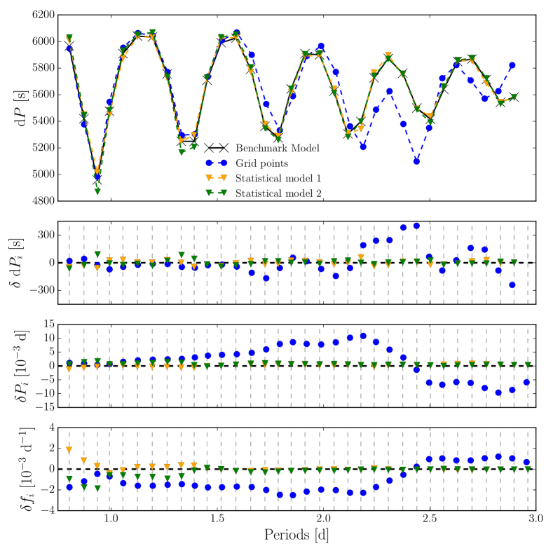
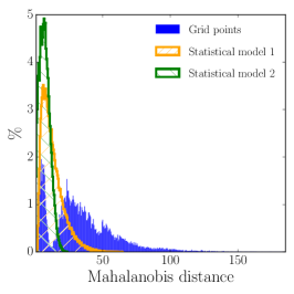
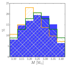
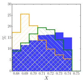
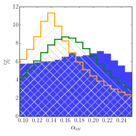
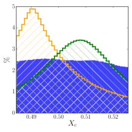
5.4 Problem 4: Stellar model selection from an ensemble of pulsators
Suppose that we have not one star as assumed so far, but rather an ensemble of stars, as well as a collection of candidate theories:
-
•
Observations , ;
-
•
Theories , .
The goal is, using all stars simultaneously, to select the most appropriate theory among the candidate theories. Using the solution to Problem 1, i.e., applying (3) to every star for every grid , we find the pair , with the fitted stellar properties for star from theory , and the predicted observation for star from theory .
The discrepancy between observed values and values predicted from theory is:
with the dispersion matrix, calculated as in (2), for the th theory. Here, the stellar models can take the form of an astrophysical model, as well as that of a statistical model built according to the principles laid out in Problem 3.
As argued above, it is again sensible to take the working view that . Let be the length of vector . Then follows a distribution, and hence as a whole follows a distribution. Using these distributions, the tail probability can be calculated. The theory with the largest fits the observed data of the ensemble of stars best.
We are not yet able to include an example of such an application, since we first must apply the above set of Problems 1, 2, 3 to a sufficient number of observed gravity-mode pulsators. This will be the subject of subsequent papers with applications of the current methodological framework.
5.5 Bayesian approach for parameter estimation
Statistical inference in asteroseismology is nowadays often done with a Bayesian approach, where the likelihood function based on data is combined with prior knowledge to update the information on the parameters and to revise the probability associated with the parameters (posterior probability). In that sense, an MLE is related to Bayesian analysis with a so-called non-informative (or flat) prior. We refer to Gruberbauer et al. (2012); Appourchaux (2014) for thorough discussions in the case of solar-like oscillations in low-mass stars, where the input physics of the model is usually taken to be very similar to the one of solar models calibrated from helioseismology. Indeed, for the “easy” case of low-mass stars with solar-like oscillations, one can make the reasonable assumption that such stars have input physics very similar to the Sun, because they are slow rotators and have a convective envelope.
In the context of gravity modes and the results obtained in Sections 2, 3, and 4, it is essential to start any Bayesian analysis with a non-informative prior about the input physics and parameters to be estimated. Given the results on theoretical uncertainties of gravity-mode frequencies of rotating stars with a convective core, as summarized in Table 2, knowledge of the choice of to be estimated and of the input physics in the model to be fixed for the stellar models has yet to be assembled for large samples of stars with a variety in mass, rotation, metalicity, and binary properties. As long as we do not know the level and shape of the interior profiles for core overshooting, rotation and chemical mixing, one should not impose insecure assumptions about these quantities, because they have a large effect on the gravity modes. For this reason, a Bayesian approach is not obvious yet for gravity-mode pulsators with a convective core, because we essentially do not have any objective prior knowledge on the choice and properties of . In this case, one should not introduce biases about the ingredients of the stellar models (cf. Table 2) but rather complete Problem 4 for samples of tens to hundreds of stars first.
However, using prior knowledge in the forward seismic modeling of gravity-mode pulsators may be applied at the level of identification of the degree and/or the azimuthal order of the gravity modes. In all of the above, we have assumed that each observed frequency has known . The occurrence of rotational splitting indeed implies unambiguous labeling of the mode wavenumbers (e.g., Kurtz et al., 2014; Saio et al., 2015; Moravveji et al., 2015), but this may not necessarily be the case when only period spacing patterns are available for mode identification (e.g., Van Reeth et al., 2016; Pápics et al., 2017; Ouazzani et al., 2017; Saio et al., 2018b). In case of ambiguity (e.g. Degroote et al., 2010; Pápics et al., 2012; Buysschaert et al., 2018), several options for should be kept open, just as for the case of solar-like oscillations with doubtful identifications (see Appourchaux, 2014, for an enlightening discussion). In this sense, model selection is ubiquitous in asteroseismology, even for the “well-known” case of solar-like oscillations, not only due to lack of secure mode identification (cf. the F-type pulsator HD 49333 as in Benomar et al., 2009; Gruberbauer et al., 2009) but also given problems in mode detection (e.g., Deheuvels et al., 2010; Corsaro & De Ridder, 2014; Davies et al., 2016). For heat-driven coherent modes, identification of and/or can sometimes be achieved from time-resolved long-term multicolour photometry and/or line-profile variations (see Aerts et al., 2010, Chapter 6, for an extensive discussion and methodology to achieve this). In case of successful empirical identification of , this information can be used as an informative prior. Lack of identification may also occur at the level of a unique value for the radial orders of each . Indeed, this labeling may be ambiguous for the regime of high-order gravity modes, given the density of the mode spectrum at low frequencies. One may then want to consider a Bayesian approach instead of MLE, so as to incorporate prior probabilities for the considering different priors of for each of the modes. The ensuing estimation methods is known as maximum a posteriori estimation.
Given that the posterior involves the likelihood function as well, its evaluation is commonly approached in a simulation-based fashion, using Monte Carlo Markov Chain (MCMC) methods (Louis & Carlin, 2009). Care has to be taken in order not to miss the best solution of the score equations (22) and (23). An optimal approach is to compare MLE and Bayesian treatments. Such comparisons in asteroseismology have been done quite extensively before (e.g. Appourchaux et al., 2012a, b), but only in the case of solar-like oscillations, where is far better known and the effect of rotation can be ignored or treated in the Ledoux approximation (e.g., Appourchaux et al., 2008; Benomar et al., 2009; Deheuvels et al., 2012; Gruberbauer et al., 2013; Appourchaux et al., 2014; Lagarde et al., 2016; Rodrigues et al., 2017; Bossini et al., 2017; Handberg et al., 2017).
Investigating MLE versus Bayesian MCMC has not been done in the context of forward seismic modeling of gravity modes. For applications to intermediate-mass or high-mass stars as treated here, interior rotation and convective core overshooting are crucial and cannot be ignored in the parameter estimation because the gravity-mode frequency values depend heavily on it. The same is true, although to a lesser extent, for chemical mixing in the gradient zone near the receding core, as this determines the mode trapping in that region. This fortunate circumstance in principle allows the properties of the core overshooting and of the near-core physics from gravity modes to be estimated, in a similar way that mode trapping properties allow the chemical profiles of white dwarf stars to be deduced (Giammichele et al., 2018). However, it does imply that we must first model an ensemble of stars without biasing prior knowledge on these uncalibrated physical phenomena.
An extensive grid-based MLE and stellar model selection procedure based on a type analysis for gravity modes and with estimation of the core overshooting parameter, was applied to the B-type gravity-mode oscillator KIC 10526294 by Moravveji et al. (2015). This MLE and model selection approach was then followed by rotation profile estimation from inversion by Triana et al. (2015), who used the AIC to deduce the most likely rotation profile. This combination of MLE for forward seismic modeling and stellar model selection from a grid-based approach, followed by statistical model selection to deduce the optimal rotation profile is the only application of its kind so far, given that Kurtz et al. (2014); Saio et al. (2015); Kallinger et al. (2017) and Szewczuk & Daszyńska-Daszkiewicz (2018) performed the modeling with simplistic parameter estimation, if at all, without considering convective overshooting as a free parameter.
6 Overall forward modeling scheme for gravity modes in rotating stars
Forward seismic modeling requires observed and identified pulsation mode frequencies and fits them with theoretically predicted frequencies deduced from stellar models. As shown in Fig. 2, it is essential to take into account the Coriolis force in the computations of the theoretical gravity-mode frequencies when performing forward seismic modeling of intermediate- and high-mass stars, even for moderate rotators. We summarize here our overall modeling scheme, including the Coriolis force that was so far ignored in the modeling, with the exception of the studies in Moravveji et al. (2016) and Schmid & Aerts (2016).
While mode frequencies are derived from space photometry, the patterns that lead to the mode identification of gravity modes as start of the modeling in absence of rotational splitting rather concern the period spacings of the modes, (cf., Fig. 12). Once mode identification has been achieved, we perform parameter estimation from the observed frequencies, because these are the measured quantities from the data. Moreover, this has the major advantage that we can easily deal with hybrid pulsators, which reveal both pressure and gravity modes, and can involve the task of searching for regularities in frequency when identifying pressure modes in addition to gravity-mode period spacing patterns (e.g., Bowman & Kurtz, 2018).
As shown by Van Reeth et al. (2016), the shape of the observed period spacings of gravito-inertial modes allows us to break down the +7D estimation problem in a multi-step approach, where the rotation frequency in the near-core region, , is estimated first by marginalizing over the other six parameters. Indeed, the near-core rotation of the star sets the “slope” of the period spacing pattern and the value of this slope turns out to be sufficiently independent of to apply a two-stage approach. Any “dips” in the tilted period spacing pattern are caused by mode trapping in the near-core region due to the value and shape of and and these can be estimated after has been derived.
Van Reeth et al. (2016) and Ouazzani et al. (2017) developed methods to estimate from the measured slope of the period spacings of gravity modes for intermediate-mass stars; the method by Van Reeth et al. (2016) was meanwhile also successfully applied to B-type pulsators (Pápics et al., 2017). With estimated, the modeling process can be continued with exploitation of the value and morphology of the observed period spacing patterns, including the structure of the dips due to mode trapping in the near-core region. In summary, we propose the following forward modeling scheme:
-
1.
Deduce the frequencies of pressure and gravity modes, and their measurement error, in both the super-inertial and sub-inertial regime, from space photometry. Select the modes revealing rotational splitting and the of that constitute period spacing patterns.
-
2.
Identify the degree and azimutal order of rotationally-split modes, whenever detected. Use the slope of the observed period spacing patterns to identify the degree and azimutal order of the gravity modes , by estimating the near-core rotation frequency , e.g., with the methods in Van Reeth et al. (2016) or Ouazzani et al. (2017). If pressure modes are identified from measured rotational splitting, deduce the rotation frequency in the stellar envelope, , from the computation of the Ledoux constant (Eqs (3.354) and (3.361) in Aerts et al., 2010). The estimation of and/or requires a sparse grid of stellar models for an appropriate range in mass, core overshoot, and metalicity and the computation of their pressure- and gravity-mode frequencies in an inertial frame of reference. This step will deliver a rough range for the mass and metalicity, as well as a narrow range for (and of if rotational splitting of pressure modes is detected).
-
3.
Compute several dedicated +7D fine grids of stellar models with free parameters mass, age, initial chemical composition, for the range of the estimated near-core rotation and its error, and for a wide range of core overshooting and envelope mixing . For the latter three quantities, assume particular shapes for their profiles: , , and also for the temperature gradient in the overshoot zone – radiative or adiabatic or a gradual transition between these two – along with fixed choices of the input physics according to Table 2 and treat those as different stellar models . For all the model grids, compute their gravity-mode frequencies and identify the radial orders of the detected modes . For each model grid , predict and estimate the parameters in +7D space, and compute the uncertainties of from MLE, following the methodology developed for Problem 1 and possibly Problem 3 in Sect. 5. The user can get a feel for the effect of different input physics on the mode frequencies and on the forward modeling in the context of correlated parameters from attacking Problem 2 for various model grids .
-
4.
Select the most likely equilibrium models following Problem 4 for each star separately (), and iterate over the scheme for an ensemble of gravity-mode pulsators. Select the overall best input physics and interpret its shortcomings vis-a-vis the ensemble of pulsators from the estimated values of the variance-covariance matrices . The latter offer a guide to improve the input physics of stellar models.
7 Conclusions
In this work, we provided a proper methodological framework to perform forward seismic modeling based on detected gravity-mode oscillation frequencies that constitue a period-spacing pattern. We allow for correlations among the parameters of the stellar models, in order to properly take into account parameter degeneracies. The method relies on the computation of the Mahalanobis distance in a grid-based approach. We focused on stars rotating up to about half their critical rotation, such that the traditional approximation provides a valid approach to compute the theoretical oscillation frequencies. The method requires gravity-mode oscillation frequencies that have been measured with a precision better than 0.001 d-1 and that can be identified in terms of their spherical degree and azimuthal order . The parameter estimation is done in a +7D parameter space for each of the fixed choices of the input physics. As a minimum, it delivers estimation of the seven parameters and their uncertainties, as well as an estimate of the variance of each of the theoretical models and its uncertainty, as a guide to improve the input physics of future stellar structure and evolution models. A major aim of our future work is to achieve an accurate mass of the helium core near the TAMS for a representative sample of gravity-mode pulsators covering a large mass range.
The methodology presented here also offers a way to replace physical model predictions of theoretical frequencies by statistical model estimations, such that cumbersome computations of ultra-fine stellar model grids can be avoided and that proper error estimation can be achieved from the paradigm of maximum likelihood estimation. A hierarchy in the importance of the physical ingredients of the stellar structure models in terms of gravity-mode frequency uncertainty was offered as guide of the modeling (Table 2).
We stress that the choice of the model parameters to estimate depends on the type of star, its rotational properties, and on the type of mode frequencies detected in the data. Before the CPU-intensive procedure of forward seismic modeling is started, the user must assemble a good understanding of the key physical ingredients of stellar structure and evolution models and their computations for the star under study. Only after proper understanding of stellar structure theory can one make a sensible choice of the free parameters to estimate from forward modeling. Our Figs 2 – 10 along with Table 2 offer a practical guideline for this choice.
In this work, we did not cover the case of close binary stars whose equilibrium models and oscillation modes are subject to tidal forces. Tides introduce deformations and/or instabilities in the interior structure of the binary components, which may be accompanied by transport of elements and of angular momentum. Moreover, tidal forces affect the solutions to the pulsation equations. This is mainly the case for gravity modes, where (near-)resonances between the frequencies of free oscillations and (multiples of) the orbit may occur. Just as for rotation and magnetism, the equilibrium models of close binaries due to tides are subject to major uncertainties. Also in this case, it is best to start forward modeling under the assumption that the tides can be treated as a secondary effect. An iterative scheme, in which a light curve and time-resolved high-precision spectroscopy covering the orbit is simultaneously solved for binarity and oscillations, will allow the oscillation frequencies to be derived. Once this has been achieved, one can perform the forward modeling as outlined here, where strong(er) (model-independent) constraints on the star can be included compared to the case of single stars. In this way, deviations between the observed oscillation frequencies and those of the optimal model by means of can be used as a guideline on how to improve the evolutionary models in terms of the missing tidal input physics.
Our formalism presented here will be applied in the near future to numerous gravity-mode pulsators found in the Kepler data, such as those in Van Reeth et al. (2016), Bowman & Kurtz (2018), and Pápics et al. (2017). Such future applications to tens of individual stars will undoubtedly improve our knowledge of the input physics of stellar evolution models, as well as pave the way to more automated applications to gravito-inertial asteroseismology. The TESS mission will offer suitable data for hundreds of gravity-mode pulsators in the mass range 1.4 – 40 M⊙ from its Continuous Viewing Zone (Ricker et al., 2016), coupled to spectroscopy (e.g., to be assembled with SDSS-V, Kollmeier et al., 2017). On the longer term, the PLATO mission will provide thousands of suitable targets for gravity-mode asteroseismology (Rauer et al., 2014).
References
- Aerts et al. (2010) Aerts, C., Christensen-Dalsgaard, J., & Kurtz, D. W. 2010, Asteroseismology, Astronomy and Astrophysics Library, Springer Berlin Heidelberg
- Aerts et al. (2014) Aerts, C., Molenberghs, G., Kenward, M. G., & Neiner, C. 2014, ApJ, 781, 88
- Aerts et al. (2003) Aerts, C., Thoul, A., Daszyńska, J., et al. 2003, Science, 300, 1926
- Aerts et al. (2017) Aerts, C., Van Reeth, T., & Tkachenko, A. 2017, ApJ, 847, L7
- Aerts et al. (2006) Aerts, C., De Cat, P., Kuschnig, R., et al. 2006, ApJ, 642, L165
- Akaike (1987) Akaike, H. 1987, Psychometrika, 52, 317. http://dx.doi.org/10.1007/BF02294359
- Angulo et al. (1999) Angulo, C., Arnould, M., Rayet, M., et al. 1999, Nuclear Physics A, 656, 3
- Appourchaux (2014) Appourchaux, T. 2014, A crash course on data analysis in asteroseismology, ed. P. L. Pallé & C. Esteban, 123
- Appourchaux et al. (2008) Appourchaux, T., Michel, E., Auvergne, M., et al. 2008, A&A, 488, 705
- Appourchaux et al. (2012a) Appourchaux, T., Benomar, O., Gruberbauer, M., et al. 2012a, A&A, 537, A134
- Appourchaux et al. (2012b) Appourchaux, T., Chaplin, W. J., García, R. A., et al. 2012b, A&A, 543, A54
- Appourchaux et al. (2014) Appourchaux, T., Antia, H. M., Benomar, O., et al. 2014, A&A, 566, A20
- Asplund et al. (2009) Asplund, M., Grevesse, N., Sauval, A. J., & Scott, P. 2009, ARA&A, 47, 481
- Ausseloos et al. (2004) Ausseloos, M., Scuflaire, R., Thoul, A., & Aerts, C. 2004, MNRAS, 355, 352
- Ball & Gizon (2017) Ball, W. H., & Gizon, L. 2017, A&A, 600, A128
- Ballot et al. (2012) Ballot, J., Lignières, F., Prat, V., Reese, D. R., & Rieutord, M. 2012, in Astronomical Society of the Pacific Conference Series, Vol. 462, Progress in Solar/Stellar Physics with Helio- and Asteroseismology, ed. H. Shibahashi, M. Takata, & A. E. Lynas-Gray, 389
- Ballot et al. (2010) Ballot, J., Lignières, F., Reese, D. R., & Rieutord, M. 2010, A&A, 518, A30
- Bellinger et al. (2016) Bellinger, E. P., Angelou, G. C., Hekker, S., et al. 2016, ApJ, 830, 31
- Benomar et al. (2009) Benomar, O., Appourchaux, T., & Baudin, F. 2009, A&A, 506, 15
- Bildsten et al. (1996) Bildsten, L., Ushomirsky, G., & Cutler, C. 1996, ApJ, 460, 827
- Bloemen et al. (2014) Bloemen, S., Hu, H., Aerts, C., et al. 2014, A&A, 569, A123
- Bossini et al. (2017) Bossini, D., Miglio, A., Salaris, M., et al. 2017, MNRAS, 469, 4718
- Bouabid et al. (2013) Bouabid, M.-P., Dupret, M.-A., Salmon, S., et al. 2013, MNRAS, 429, 2500
- Bowman (2017) Bowman, D. M. 2017, Amplitude Modulation of Pulsation Modes in Delta Scuti Stars, Jeremiah Horrocks Institute, University of Central Lancashire, Preston, UK. PhD Thesis published in Springer Theses series, doi:10.1007/978-3-319-66649-5
- Bowman & Kurtz (2018) Bowman, D. M., & Kurtz, D. W. 2018, MNRAS, 476, 3169
- Bowman et al. (2016) Bowman, D. M., Kurtz, D. W., Breger, M., Murphy, S. J., & Holdsworth, D. L. 2016, MNRAS, 460, 1970
- Braithwaite (2009) Braithwaite, J. 2009, MNRAS, 397, 763
- Brassard et al. (2001) Brassard, P., Fontaine, G., Billères, M., et al. 2001, ApJ, 563, 1013
- Breger et al. (1999) Breger, M., Pamyatnykh, A. A., Pikall, H., & Garrido, R. 1999, A&A, 341, 151
- Breger et al. (1993) Breger, M., Stich, J., Garrido, R., et al. 1993, A&A, 271, 482
- Briquet et al. (2011) Briquet, M., Aerts, C., Baglin, A., et al. 2011, A&A, 527, A112
- Briquet et al. (2012) Briquet, M., Neiner, C., Aerts, C., et al. 2012, MNRAS, 427, 483
- Buchler et al. (1997) Buchler, J. R., Goupil, M.-J., & Hansen, C. J. 1997, A&A, 321, 159
- Buysschaert et al. (2018) Buysschaert, B., Aerts, C., Bowman, D. M., et al. 2018, A&A, in press, arXiv:1805.00802
- Cameron et al. (2008) Cameron, C., Saio, H., Kuschnig, R., et al. 2008, ApJ, 685, 489
- Chaplin & Miglio (2013) Chaplin, W. J., & Miglio, A. 2013, ARA&A, 51, 353
- Chapman & Lindzen (1970) Chapman, S., & Lindzen, R. 1970, Atmospheric tides. Thermal and gravitational
- Charpinet et al. (2011) Charpinet, S., Van Grootel, V., Fontaine, G., et al. 2011, A&A, 530, A3
- Claeskens & Hjort (2008) Claeskens, G., & Hjort, N. L. 2008, Model Selection and Model Averaging, Cambridge Series in Statistical and Probabilistic Mathematics
- Claret & Torres (2017) Claret, A., & Torres, G. 2017, ApJ, 849, 18
- Corsaro & De Ridder (2014) Corsaro, E., & De Ridder, J. 2014, A&A, 571, A71
- Córsico et al. (2012) Córsico, A. H., Romero, A. D., Althaus, L. G., & Hermes, J. J. 2012, A&A, 547, A96
- Cowling (1941) Cowling, T. G. 1941, MNRAS, 101, 367
- Cox & Hinkley (1990) Cox, D., & Hinkley, D. 1990, Theoretical Statistics, London: CRC/Chapman & Hall
- Daszyńska-Daszkiewicz et al. (2017) Daszyńska-Daszkiewicz, J., Pamyatnykh, A. A., Walczak, P., et al. 2017, MNRAS, 466, 2284
- Daszyńska-Daszkiewicz & Walczak (2010) Daszyńska-Daszkiewicz, J., & Walczak, P. 2010, MNRAS, 403, 496
- Davies et al. (2016) Davies, G. R., Silva Aguirre, V., Bedding, T. R., et al. 2016, MNRAS, 456, 2183
- De Ridder et al. (2004) De Ridder, J., Telting, J. H., Balona, L. A., et al. 2004, MNRAS, 351, 324
- Deal et al. (2017) Deal, M., Escobar, M. E., Vauclair, S., et al. 2017, A&A, 601, A127
- Deal et al. (2016) Deal, M., Richard, O., & Vauclair, S. 2016, A&A, 589, A140
- Degroote et al. (2009) Degroote, P., Briquet, M., Catala, C., et al. 2009, A&A, 506, 111
- Degroote et al. (2010) Degroote, P., Aerts, C., Baglin, A., et al. 2010, Nature, 464, 259
- Deheuvels et al. (2016) Deheuvels, S., Brandão, I., Silva Aguirre, V., et al. 2016, A&A, 589, A93
- Deheuvels et al. (2010) Deheuvels, S., Bruntt, H., Michel, E., et al. 2010, A&A, 515, A87
- Deheuvels et al. (2012) Deheuvels, S., García, R. A., Chaplin, W. J., et al. 2012, ApJ, 756, 19
- Dotter et al. (2017) Dotter, A., Conroy, C., Cargile, P., & Asplund, M. 2017, ApJ, 840, 99
- Dupret et al. (2005) Dupret, M.-A., Grigahcène, A., Garrido, R., Gabriel, M., & Scuflaire, R. 2005, A&A, 435, 927
- Dupret et al. (2004) Dupret, M.-A., Thoul, A., Scuflaire, R., et al. 2004, A&A, 415, 251
- Dziembowski & Krolikowska (1985) Dziembowski, W., & Krolikowska, M. 1985, Acta Astron., 35, 5
- Dziembowski et al. (2007) Dziembowski, W. A., Daszyńska-Daszkiewicz, J., & Pamyatnykh, A. A. 2007, MNRAS, 374, 248
- Dziembowski & Goode (1996) Dziembowski, W. A., & Goode, P. R. 1996, ApJ, 458, 338
- Dziembowski & Pamyatnykh (2008) Dziembowski, W. A., & Pamyatnykh, A. A. 2008, MNRAS, 385, 2061
- Eckart (1960) Eckart, C. 1960, Physics of Fluids, 3, 421
- Eggenberger et al. (2017) Eggenberger, P., Lagarde, N., Miglio, A., et al. 2017, A&A, 599, A18
- Geroux & Deupree (2013) Geroux, C. M., & Deupree, R. G. 2013, ApJ, 771, 113
- Giammichele et al. (2017) Giammichele, N., Charpinet, S., Brassard, P., & Fontaine, G. 2017, A&A, 598, A109
- Giammichele et al. (2018) Giammichele, N., Charpinet, S., Fontaine, G., et al. 2018, Nature, 554, 73
- Gruberbauer et al. (2012) Gruberbauer, M., Guenther, D. B., & Kallinger, T. 2012, ApJ, 749, 109
- Gruberbauer et al. (2013) Gruberbauer, M., Guenther, D. B., MacLeod, K., & Kallinger, T. 2013, MNRAS, 435, 242
- Gruberbauer et al. (2009) Gruberbauer, M., Kallinger, T., Weiss, W. W., & Guenther, D. B. 2009, A&A, 506, 1043
- Handberg et al. (2017) Handberg, R., Brogaard, K., Miglio, A., et al. 2017, MNRAS, 472, 979
- Handler (2009) Handler, G. 2009, MNRAS, 398, 1339
- Handler et al. (2006) Handler, G., Jerzykiewicz, M., Rodríguez, E., et al. 2006, MNRAS, 365, 327
- Handler et al. (2009) Handler, G., Matthews, J. M., Eaton, J. A., et al. 2009, ApJ, 698, L56 (3)
- Heger et al. (2000) Heger, A., Langer, N., & Woosley, S. E. 2000, ApJ, 528, 368
- Hekker & Christensen-Dalsgaard (2017) Hekker, S., & Christensen-Dalsgaard, J. 2017, A&A Rev., 25, 1
- Hermes et al. (2017) Hermes, J. J., Kawaler, S. D., Romero, A. D., et al. 2017, ApJ, 841, L2
- Hu et al. (2011) Hu, H., Tout, C. A., Glebbeek, E., & Dupret, M.-A. 2011, MNRAS, 418, 195
- Johnson & Wichern (2002) Johnson, R., & Wichern, D. 2002, Applied Multivariate Statistical Analyis (Upper Saddle River, NJ: Prentice-Hall)
- Johnson & Wichern (2000) Johnson, R. A., & Wichern, D. W. 2000, Applied Multivariate Statistical Analysis, 4th Edition, Englewood Cliffs, Prentice-Hall
- Kallinger et al. (2017) Kallinger, T., Weiss, W. W., Beck, P. G., et al. 2017, A&A, 603, A13
- Kass & Raftery (1995) Kass, R., & Raftery, A. 1995, Journal of the American Statistical Association, 90, 773
- Kippenhahn et al. (2012) Kippenhahn, R., Weigert, A., & Weiss, A. 2012, Stellar Structure and Evolution, doi:10.1007/978-3-642-30304-3
- Kollmeier et al. (2017) Kollmeier, J. A., Zasowski, G., Rix, H.-W., et al. 2017, SDSS-V Instrument Paper, arXiv:1711.03234
- Kudritzki & Puls (2000) Kudritzki, R.-P., & Puls, J. 2000, ARA&A, 38, 613
- Kurtz et al. (2014) Kurtz, D. W., Saio, H., Takata, M., et al. 2014, MNRAS, 444, 102
- Lagarde et al. (2016) Lagarde, N., Bossini, D., Miglio, A., Vrard, M., & Mosser, B. 2016, MNRAS, 457, L59
- Lai (1997) Lai, D. 1997, ApJ, 490, 847
- Ledoux (1951) Ledoux, P. 1951, ApJ, 114, 373
- Lee & Baraffe (1995) Lee, U., & Baraffe, I. 1995, A&A, 301, 419
- Louis & Carlin (2009) Louis, T. L., & Carlin, B. P. 2009, Bayesian Methods for Data Analysis, Boca Raton, FL: Chapman & Hall/CRC
- Loumos & Deeming (1978) Loumos, G. L., & Deeming, T. J. 1978, Ap&SS, 56, 285
- Martins et al. (2012a) Martins, F., Escolano, C., Wade, G. A., et al. 2012a, A&A, 538, A29
- Martins et al. (2012b) Martins, F., Mahy, L., Hillier, D. J., & Rauw, G. 2012b, A&A, 538, A39
- Mathis (2013) Mathis, S. 2013, in Lecture Notes in Physics, Berlin Springer Verlag, Vol. 865, Lecture Notes in Physics, Berlin Springer Verlag, ed. M. Goupil, K. Belkacem, C. Neiner, F. Lignières, & J. J. Green, 23
- Michaud et al. (2004) Michaud, G., Richard, O., Richer, J., & VandenBerg, D. A. 2004, ApJ, 606, 452
- Miglio & Montalbán (2005) Miglio, A., & Montalbán, J. 2005, A&A, 441, 615
- Miglio et al. (2012) Miglio, A., Brogaard, K., Stello, D., et al. 2012, MNRAS, 419, 2077
- Molenberghs & Verbeke (2005) Molenberghs, G., & Verbeke, G. 2005, Models for Discrete Longitudinal Data, New York: Springer
- Moravveji et al. (2015) Moravveji, E., Aerts, C., Pápics, P. I., Triana, S. A., & Vandoren, B. 2015, A&A, 580, A27
- Moravveji et al. (2016) Moravveji, E., Townsend, R. H. D., Aerts, C., & Mathis, S. 2016, ApJ, 823, 130
- Morel et al. (2008) Morel, T., Hubrig, S., & Briquet, M. 2008, A&A, 481, 453
- Nash (1990) Nash, J. C. 1990, The Choleski Decomposition, in: Compact Numerical Methods for Computers: Linear Algebra and Function Minimisation, 2nd ed. Bristol, England: Adam Hilger
- Neiner et al. (2009) Neiner, C., Gutiérrez-Soto, J., Baudin, F., et al. 2009, A&A, 506, 143
- Neter & Kutner (1990) Neter, J. Wasserman, W., & Kutner, M. 1990, Applied Linear Statistical Models. Regression, Analysis of Variance and Experimental Designs, 3rd ed., Homewood, IL: Richard D. Irwin, Inc.
- Nowakowski (2005) Nowakowski, R. M. 2005, Acta Astron., 55, 1
- Ouazzani et al. (2018) Ouazzani, R.-M., Marques, J. P., Goupil, M.-J., et al. 2018, A&A, submitted
- Ouazzani et al. (2017) Ouazzani, R.-M., Salmon, S. J. A. J., Antoci, V., et al. 2017, MNRAS, 465, 2294
- Pablo et al. (2016) Pablo, H., Whittaker, G. N., Popowicz, A., et al. 2016, PASP, 128, 125001
- Pápics et al. (2014) Pápics, P. I., Moravveji, E., Aerts, C., et al. 2014, A&A, 570, A8
- Pápics et al. (2012) Pápics, P. I., Briquet, M., Baglin, A., et al. 2012, A&A, 542, A55
- Pápics et al. (2017) Pápics, P. I., Tkachenko, A., Van Reeth, T., et al. 2017, A&A, 598, A74
- Paxton et al. (2011) Paxton, B., Bildsten, L., Dotter, A., et al. 2011, ApJS, 192, 3
- Paxton et al. (2013) Paxton, B., Cantiello, M., Arras, P., et al. 2013, ApJS, 208, 4
- Paxton et al. (2015) Paxton, B., Marchant, P., Schwab, J., et al. 2015, ApJS, 220, 15
- Paxton et al. (2018) Paxton, B., Schwab, J., Bauer, E. B., et al. 2018, ApJS, 234, 34
- Pedersen et al. (2018) Pedersen, M. G., Aerts, C., Pápics, P. I., & Rogers, T. M. 2018, A&A, in press, arXiv:1802.02051
- Penrose (1955) Penrose, R. 1955, Proceedings of the Cambridge Philosophical Society, 51, 406
- Poretti et al. (2009) Poretti, E., Michel, E., Garrido, R., et al. 2009, A&A, 506, 85
- Przybilla et al. (2013) Przybilla, N., Nieva, M. F., Irrgang, A., & Butler, K. 2013, in EAS Publications Series, Vol. 63, EAS Publications Series, ed. G. Alecian, Y. Lebreton, O. Richard, & G. Vauclair, 13–23
- Puls et al. (2005) Puls, J., Urbaneja, M. A., Venero, R., et al. 2005, A&A, 435, 669
- Quirion et al. (2010) Quirion, P.-O., Christensen-Dalsgaard, J., & Arentoft, T. 2010, ApJ, 725, 2176
- Rauer et al. (2014) Rauer, H., Catala, C., Aerts, C., et al. 2014, Experimental Astronomy, 38, 249
- Reese et al. (2006) Reese, D., Lignières, F., & Rieutord, M. 2006, A&A, 455, 621
- Richer et al. (2000) Richer, J., Michaud, G., & Turcotte, S. 2000, ApJ, 529, 338
- Ricker et al. (2016) Ricker, G. R., Vanderspek, R., Winn, J., et al. 2016, in Proc. SPIE, Vol. 9904, Space Telescopes and Instrumentation 2016: Optical, Infrared, and Millimeter Wave, 99042B
- Rieutord et al. (2016) Rieutord, M., Espinosa Lara, F., & Putigny, B. 2016, Journal of Computational Physics, 318, 277
- Rodrigues et al. (2017) Rodrigues, T. S., Bossini, D., Miglio, A., et al. 2017, MNRAS, 467, 1433
- Rogers (2015) Rogers, T. M. 2015, ApJ, 815, L30
- Rogers & McElwaine (2017) Rogers, T. M., & McElwaine, J. N. 2017, ApJ, 848, L1
- Romero et al. (2017) Romero, A. D., Córsico, A. H., Castanheira, B. G., et al. 2017, ApJ, 851, 60
- Royston & Altman (1994) Royston, P., & Altman, D. 1994, Applied Statistics, 43, 429
- Royston & Sauerbrei (2008) Royston, P., & Sauerbrei, W. 2008, Multivariable Model Building: A pragmatic approach to regression analysis based on fractional polynomials for modelling continuous variables. John Wiley & Sons, Chichester
- Saio (1981) Saio, H. 1981, ApJ, 244, 299
- Saio et al. (2018a) Saio, H., Bedding, T. R., Kurtz, D. W., et al. 2018a, MNRAS, 477, 2183
- Saio et al. (2018b) Saio, H., Kurtz, D. W., Murphy, S. J., Antoci, V. L., & Lee, U. 2018b, MNRAS, 474, 2774
- Saio et al. (2015) Saio, H., Kurtz, D. W., Takata, M., et al. 2015, MNRAS, 447, 3264
- Saio et al. (2006) Saio, H., Kuschnig, R., Gautschy, A., et al. 2006, ApJ, 650, 1111
- Salaris & Cassisi (2017) Salaris, M., & Cassisi, S. 2017, Royal Society Open Science, 4, 170192
- Santolaya-Rey et al. (1997) Santolaya-Rey, A. E., Puls, J., & Herrero, A. 1997, A&A, 323, 488
- Sauerbrei & Royston (1999) Sauerbrei, W., & Royston, P. 1999, Journal of the Royal Statistical Society, Series A, 162, 71
- Schmid & Aerts (2016) Schmid, V. S., & Aerts, C. 2016, A&A, 592, A116
- Schwarz (1978) Schwarz, G. 1978, Annals of Statistics, 6, 461
- Seber & Wild (2003) Seber, G., & Wild, C. 2003, Nonlinear Regression, New York: John Wiley & Sons
- Silva Aguirre et al. (2017) Silva Aguirre, V., Lund, M. N., Antia, H. M., et al. 2017, ApJ, 835, 173
- Smolec & Moskalik (2007) Smolec, R., & Moskalik, P. 2007, MNRAS, 377, 645
- Sowicka et al. (2017) Sowicka, P., Handler, G., Dȩbski, B., et al. 2017, MNRAS, 467, 4663
- Szewczuk & Daszyńska-Daszkiewicz (2017) Szewczuk, W., & Daszyńska-Daszkiewicz, J. 2017, MNRAS, 469, 13
- Szewczuk & Daszyńska-Daszkiewicz (2018) —. 2018, MNRAS, in press, arXiv:1805.07100
- Tayar & Pinsonneault (2013) Tayar, J., & Pinsonneault, M. H. 2013, ApJ, 775, L1
- Townsend (2000a) Townsend, R. H. D. 2000a, MNRAS, 318, 1
- Townsend (2000b) —. 2000b, MNRAS, 319, 289
- Townsend (2003a) —. 2003a, MNRAS, 340, 1020
- Townsend (2003b) —. 2003b, MNRAS, 343, 125
- Townsend et al. (2018) Townsend, R. H. D., Goldstein, J., & Zweibel, E. G. 2018, MNRAS, 475, 879
- Townsend & Teitler (2013) Townsend, R. H. D., & Teitler, S. A. 2013, MNRAS, 435, 3406
- Trampedach et al. (2017) Trampedach, R., Aarslev, M. J., Houdek, G., et al. 2017, MNRAS, 466, L43
- Triana et al. (2015) Triana, S. A., Moravveji, E., Pápics, P. I., et al. 2015, ApJ, 810, 16
- Truyaert (2016) Truyaert, K. 2016, Master Thesis, KU Leuven, Belgium
- Turcotte et al. (1998) Turcotte, S., Richer, J., & Michaud, G. 1998, ApJ, 504, 559
- Unno et al. (1989) Unno, W., Osaki, Y., Ando, H., Saio, H., & Shibahashi, H. 1989, Nonradial oscillations of stars
- Van Reeth et al. (2016) Van Reeth, T., Tkachenko, A., & Aerts, C. 2016, A&A, 593, A120
- Van Reeth et al. (2015) Van Reeth, T., Tkachenko, A., Aerts, C., et al. 2015, ApJS, 218, 27
- Verbeke & Molenberghs (2000) Verbeke, G., & Molenberghs, G. 2000, Linear Mixed Models for Longitudinal Data. New York: Springer
- Verma et al. (2017) Verma, K., Raodeo, K., Antia, H. M., et al. 2017, ApJ, 837, 47
- Wade et al. (2016) Wade, G. A., Neiner, C., Alecian, E., et al. 2016, MNRAS, 456, 2
- Walker et al. (2005) Walker, G. A. H., Kuschnig, R., Matthews, J. M., et al. 2005, ApJ, 635, L77
- Welsh (1996) Welsh, A. 1996, Aspects of Statistical Inference, New York: John Wiley & Sons
- White (1982) White, H. 1982, Econometrica, 50, 1
- Zorec & Royer (2012) Zorec, J., & Royer, F. 2012, A&A, 537, A120
- Zwintz et al. (2013) Zwintz, K., Fossati, L., Guenther, D. B., et al. 2013, A&A, 552, A68
- Zwintz et al. (2014) Zwintz, K., Fossati, L., Ryabchikova, T., et al. 2014, Science, 345, 550
- Zwintz et al. (2017) Zwintz, K., Moravveji, E., Pápics, P. I., et al. 2017, A&A, 601, A101
Appendix A MESA and GYRE inlists
Example MESA and GYRE inlists used for this work are available from the MESA Inlists section of the MESA Marketplace: cococubed.asu.edu/mesa-market/inlists.html
In addition, a MESA/GYRE
tutorial on gravity-mode asteroseismology can be retrieved from the Education
section, MESA summer school year 2016:
cococubed.asu.edu/mesa-market/education.html
Appendix B Solving the score equations in the case of non-linear statistical models with fractional polynomials
The aim in Problem 3 is to solve the score equations and derive optimal values for . The general case of non-linear statistical models to do so may be quite challenging, although necessary in the case that linear models do not offer a proper fit. Although classical polynomial predictors are still very customary and relatively easy to use, they are often inadequate because quickly very high-degree polynomials are needed, resulting in poor predictive properties. This can in principle be overcome by using predictor functions that are non-linear in the parameters. However, such models, in turn, are often ridden with computational challenges. Therefore, we would like to point to a model family that shares with polynomial methods the ease of fitting because it still is part of the generalized linear models family, on the one hand, and that shares with non-linear models the flexibility of describing a wide array of functions. This family is called “fractional polynomials” and was advocated by Royston & Altman (1994).
A broad overview of the use and applications of this method in a variety of statistical areas can be found in Royston & Sauerbrei (2008). Several uses in hierarchical data structures are described in Verbeke & Molenberghs (2000) and Molenberghs & Verbeke (2005).
For a given degree and a univariate argument , fractional polynomials are defined as
where the are regression parameters, if and . The powers are either positive or negative integers, or fractions. Royston & Altman (1994) argue that polynomials with degree higher than 2 are rarely required in practice and further restrict the powers of to a small pre-defined set of noninteger values:
The full definition includes possible “repeated powers” which involve multiplication with . For example, a fractional polynomial of degree with powers (,,2) is of the form (Royston & Altman, 1994; Sauerbrei & Royston, 1999). Setting , for example, will generate:
-
(1)
“quadratics” in powers of , represented by
-
–
,
-
–
,
-
–
, and
-
–
;
-
–
-
(2)
a quadratic in : ; and
-
(3)
several other curves with shapes different from those of low degree polynomials.
For given , we consider as the best set of transformations, the one producing the highest log-likelihood. For example, the best first degree fractional polynomial is the one with the highest log-likelihood among the eight models with one regressor (). As with conventional polynomials, the degree is selected either informally on a priori grounds or by increasing until no worthwhile improvement in the fit of the best fitting fractional polynomial occurs. In the above discussion, it is assumed that is strictly positive. If can take zero values, a preliminary transformation of is needed to ensure positivity (e.g., ).
Evidently, the in our case would be a component of . Given that there are typically several components in , the ideas above can be applied to all components simultaneously. This may give rise to a large set of possible predictors.