Quantile Regression of Latent Longitudinal

Trajectory Features

Huijuan Ma¹, Limin Peng¹ and Haoda Fu²

¹Department of Biostatistics and Bioinformatics, Emory University

²Eli Lilly and Company

Abstract: Quantile regression has demonstrated promising utility in longitudinal data analysis. Existing work is primarily focused on modeling cross-sectional outcomes, while outcome trajectories often carry more substantive information in practice. In this work, we develop a trajectory quantile regression framework that is designed to robustly and flexibly investigate how latent individual trajectory features are related to observed subject characteristics. The proposed models are built under multilevel modeling with usual parametric assumptions lifted or relaxed. We derive our estimation procedure by novelly transforming the problem at hand to quantile regression with perturbed responses and adapting the bias correction technique for handling covariate measurement errors. We establish desirable asymptotic properties of the proposed estimator, including uniform consistency and weak convergence. Extensive simulation studies confirm the validity of the proposed method as well as its robustness. An application to the DURABLE trial uncovers sensible scientific findings and illustrates the practical value of our proposals.

Keywords: Corrected loss function; Latent longitudinal trajectory; Longitudinal quantile regression; Multilevel modeling.

1 Introduction

Longitudinal data, characterized by repeated measurements from the same subject, provide the essential platform for exploiting the temporal patterns of scientific outcomes. Such data frequently arise in biomedical research. A general account of methods for analyzing longitudinal data can be found in various texts (Jones, 1993; Hand and Crowder, 1996; Verbeke and Molenberghs, 2000; Diggle et al., 2002; Fitzmaurice et al., 2004, among others).

Quantile regression (Koenker and Bassett, 1978), given its robustness in handling skewed responses and flexibility in characterizing covariate effects, has demonstrated promising utility in longitudinal data analysis. A common way to formulate longitudinal quantile regression is to specify the outcome quantile at a given time point as a function of covariates, sharing a similar spirit with the generalized estimating equation (GEE) approach (Liang and Zeger, 1986). A number of authors have studied such a marginal quantile regression model, including the GEE-type estimating equations and empirical-likelihood approaches (Jung, 1996; He et al., 2003; Chen et al., 2004; Fu and Wang, 2012; Leng and Zhang, 2014; Lu and Fan, 2015, among others). Extensions have also been proposed to address data complications such as dropouts and censoring (Lipsitz et al., 1997; Wang and Fygenson, 2009; Lee and Kong, 2013; Sun et al., 2016, for example). A more flexible modeling strategy for longitudinal quantile regression is to model outcome quantiles conditioning on covariates as well as fixed or random individual parameters that capture unobserved heterogeneity. Such conditional quantile regression models provide individual-specific interpretations and can be estimated through distribution-free or likelihood-based approaches (Koenker, 2004; Harding and Lamarche, 2009; Galvao and Montes-Rojas, 2010; Galvao, 2011, among others). It is worth noting that all these existing models are oriented to infer about the quantiles of the longitudinal outcome at given time points (i.e. cross-sectional quantiles).

In practice, there are many practical scenarios where the scientific interest pertains to the within-subject trajectory of an outcome. To address such an interest, the current modeling of cross-sectional quantiles may not suffice because the changing pattern of cross-sectional quantiles over time often do not reflect the outcome changing pattern at the subject level. For example, in the DURABLE trial (Buse et al., 2009) that evaluated two starter insulin regimens in type 2 diabetes patients, how quickly HbA1c decreases over time within a patient may be a more substantive efficacy measure than the patient’s HbA1c level at each follow-up visit. This is because the trajectory of HbA1c would better inform us the patient’s early response of treatment which is an effective indicator of the likely need for change in (or intensification of) therapy (Fu et al., 2015). As shown by Fig. 1, the 25th, 50th, and 75th cross-sectional quartiles of HbA1c are all decreasing with time (see black solid lines), while examining the within-subject data suggests that some subjects may have underlying HbA1c trajectories roughly unchanged or even increasing over time (see red dotted lines). These subjects correspond to weak responders to the assigned insulin treatment, which is of critical clinical importance but cannot be captured by evaluating the temporal trend of the cross-sectional quantiles.

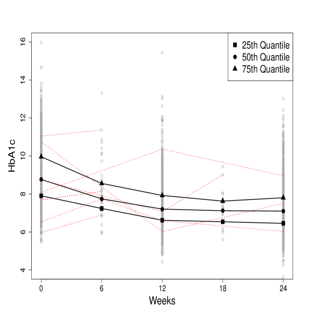
Figure 1: DURABLE trial: HbA1c values over time. The solid black lines depict the 25th, 50th, and 75th quantiles of HbA1c at different time points; the red dotted lines examplify the HbA1c trajectories of 5 subjects.

It is remarkable that the trajectory-related measures, such as the decreasing rate of within-subject HbA1c values, unlike the cross-sectional measurements, are not directly observable but may be accessible through trajectory modeling of HbA1c at the individual level. To investigate whether and how a certain insulin treatment or individual characteristics lead to more rapid reductions of HbA1c, a natural approach is to consider multilevel modeling (MLM) (Raudenbush and Bryk, 2002). That is, one may assume a level-1 trajectory model for the repeated HbA1c measurements within each subject, and then use a level-2 model to link covariates with the latent individual-specific features that capture the HbA1c reduction pattern based on the level-1 model. Traditional MLM for longitudinal data (or repeated measures) generally adopts i.i.d. normal random errors at every level of the model (Snijders and Bosker, 2002; Hedeker, 2006, for example). While this assumption helps ensure the model identifiability and facilitates likelihood-based inferences, it can induce potentially stringent data constraints. Integrating quantile regression into repeated measures MLM, for example in the level-2 model described above, can avoid some of unverifiable distributional assumptions. It can also offer the same flexibility to explore meaningful heterogeneous covariate effects as in the standard quantile regression.

In this paper, we propose a new longitudinal quantile regression framework that serves to investigate individual trajectory features of longitudinal data under MLM. We shall refer the new framework to as longitudinal trajectory quantile regression. Our new model is easy to interpret, and complements the current marginal or conditional quantile regression models that are focused on the cross-sectional quantiles. As a proof of concept, we illustrate in Section 2 the proposed framework assuming a polynomial trajectory model and taking the outcome changing rate as the targeted trajectory feature. The main thrust of our method is to deal with unobserved latent responses (e.g. decreasing rate of HbA1c) in the quantile regression context without fully parametric modeling. Our key strategy is to map the latent quantile regression model to a quantile regression problem with observed but perturbed responses. As delineated in Section 3, we show that the bias caused by the response perturbance can be corrected through adapting the technique for handling covariate measurement errors (Stefanski and Carroll, 1990; Wang et al., 2012). Our estimation method permits a less restrictive trajectory model for the correlated within-subject measurements, for example, by allowing the error term to be non-normal. We carefully examine the developed inference procedures including the associated asymptotic properties and computational features; see Section 4. Our simulations reported in Section 5 confirm the validity of the proposed longitudinal trajectory quantile regression procedures and demonstrate their satisfactory performance with finite sample sizes. The data application presented in Section 6 represents a novel secondary analysis of the DURABLE study, which reveals more robust and detailed heterogeneity patterns in longitudinal HbA1c outcomes.

2 The Proposed Longitudinal Trajectory Quantile Regression Framework

Consider a longitudinal study that consists of $n$ subjects. For subject $i$, let $Y_{i}(t)$ denote the outcome variable of interest. We adopt a polynomial trajectory model for $Y_{i}(t)$ that takes the general form,

$$Y_{i}(t)=f(t;\boldsymbol{\alpha}_{i})+\epsilon_{i}(t)\doteq\sum_{j=0}^{k}\alpha_{ij}t^{j}+\epsilon_{i}(t),$$ (2.1)

where $f(t;\boldsymbol{\alpha}_{i})$ is a $k$-th order polynomial function of time $t$, $\boldsymbol{\alpha}_{i}=(\alpha_{i0},\alpha_{i1},\ldots,\alpha_{ik})^{\!\top\!}$ is an unknown random parameter vector, and $\epsilon_{i}(t)$ is a mean zero process independent of $\boldsymbol{\alpha}_{i}$. Here the random parameters in $\boldsymbol{\alpha}_{i}$ are not subject to the mean zero constraint and so they are general enough to capture both the fixed and random effects (of covariates) on $Y_{i}(t)$. Under model (2.1), $f(t;\boldsymbol{\alpha}_{i})$ represents the underlying outcome trajectory of interest for subject $i$ determined by $\boldsymbol{\alpha}_{i}$, and $\epsilon_{i}(t)$ may play a role like a random noise or measurement error.

Remark 1: It is important to point out that the main interest under model (2.1) is the underlying trajectory for subject $i$, $f(t;\boldsymbol{\alpha}_{i})$, and is not the conditional mean of $Y_{i}(t)$ given a covariate vector, say $\boldsymbol{X}_{i}$, i.e. $E(Y_{i}(t)|\boldsymbol{X}_{i})\equiv E(f(t;\boldsymbol{\alpha}_{i})|\boldsymbol{X}_{i})$. This distinguishes model (2.1) from the traditional conditional mean modeling of longitudinal data.

The polynomial specification of $f(\cdot)$ can flexibly characterize various types of outcome temporal patterns. At the same time it provides the technical convenience that allows a meaningful trajectory-related feature of interest, denoted by $B_{i}$, be represented as a known parametric function of $\boldsymbol{\alpha}_{i}$, $\phi(\boldsymbol{\alpha}_{i})$. With real data, the polynomial order $k$ may be determined by examining the observed within-subject longitudinal measurements. As motivated by the application to the DURABLE trial, we consider the special case where $\phi(\boldsymbol{\alpha}_{i})$ corresponds to the changing rate of the within-subject outcome trajectory at a given time point $t_{*}$, which, under model (2.1), takes the form

$$B_{i}\doteq\phi(\boldsymbol{\alpha}_{i})=\frac{\partial f(t;\boldsymbol{\alpha}_{i})}{\partial t}\bigg{|}_{t=t_{*}}=\sum_{j=1}^{k}j\alpha_{ij}t_{*}^{j-1}.$$ (2.2)

When $k=1$, $B_{i}$ is simply $\alpha_{i1}$, the random slope of the assumed linear trajectory. In practice, $t_{*}$ is often pre-specified per study protocol. Studying other forms of $\phi(\cdot)$, such as the area under curve of $Y_{i}(t)$ in a given time interval, can be carried out based on the same strategy presented in this work.

The focus of the proposed framework is to use quantile regression to permit a robust and comprehensive examination of the relationship between a latent outcome trajectory feature and the observed covariates. Let $\tilde{\boldsymbol{X}}$ denote a $(p-1)\times 1$ vector of covariates, $\boldsymbol{X}=(1,\tilde{\boldsymbol{X}}^{\!\top\!})^{\!\top\!}$, and let $B$ stand for the population analogue of $B_{i}$. The $\tau$th conditional quantile of $B$ given $\boldsymbol{X}$ is defined as $Q_{B}(\tau|\boldsymbol{X})\doteq\inf\{b:\ \Pr(B\leq b|\boldsymbol{X})\geq\tau\}$. We assume the following quantile regression model:

$$Q_{B}(\tau|\boldsymbol{X})=\boldsymbol{X}^{\!\top\!}\boldsymbol{\beta}_{0}(\tau),$$ (2.3)

where $\tau\in(0,1)$ and $\boldsymbol{\beta}_{0}(\tau)\in\mathcal{R}^{p}$ is an unknown coefficient vector. The coefficients in $\boldsymbol{\beta}_{0}(\tau)$, as interpreted in the standard quantile regression (Koenker, 2005), reveal the change in the $\tau$-th quantile of $B$ per one unit covariate change. When all non-intercept coefficients in $\boldsymbol{\beta}_{0}(\tau)$ are constant, model (2.3) reduces to a linear model where the regression coefficients represent the location shift to the distribution of $B$ resulted from one unit covariate change.

Models (2.1) and (2.3) together can be viewed as a multilevel model with level-1 units consisting of the repeated measurements for each subject and level-2 units corresponding to subjects. The multilevel model perspective enables us to employ quantile regression to investigate the determinants of a latent trajectory feature of interest. The resulting multilevel model encompasses common repeated measures models such as linear mixed model with random intercept or slope. The quantile regression specification of the level-2 model avoids some of usual normality assumptions involved in the linear mixed models and hence leads to improved robustness.

3 The Proposed Estimation

In longitudinal studies, the outcome process $Y_{i}(t)$ is usually not continuously observed; rather $Y_{i}(t)$ is measured only at multiple discrete time points, say $t_{i1}<t_{i2}<\cdots<t_{im_{i}}$, where $m_{i}$ is the total number of observations for subject $i$. Let $Y_{ij}$ denote the $Y(t)$ measured for subject $i$ at time point $t_{ij}$. The observed data consist of $\{Y_{ij},t_{ij},\boldsymbol{X}_{i}:j=1,\ldots,m_{i};~{}i=1,\ldots,n\}$. Our data scenario accommodates both regular and irregular time points for longitudinal measurements.

Model (2.1) implies that $Y_{ij}=\alpha_{i0}+\alpha_{i1}t_{ij}+\alpha_{i2}t_{ij}^{2}+\ldots+\alpha_{ik}t_{ij}^{k}+\epsilon_{ij}$ with $\epsilon_{ij}=\boldsymbol{\epsilon}_{i}(t_{ij})$ for $j=1,\ldots,m_{i}$ and $i=1,\ldots,n$. This can further be expressed in a matrix form,

$${\bf Y}_{i}=\boldsymbol{Z}_{i}\boldsymbol{\alpha}_{i}+\boldsymbol{\epsilon}_{i},$$ (3.4)

where ${\bf Y}_{i}=(Y_{i1},\ldots,Y_{im_{i}})^{\!\top\!}$, $\boldsymbol{Z}_{i}=(z_{p,q})$ is a $m_{i}\times(k+1)$ matrix with $z_{p,q}=t_{ip}^{q-1}$, and $\boldsymbol{\epsilon}_{i}=(\epsilon_{i1},\ldots,\epsilon_{im_{i}})^{\!\top\!}$, and $\boldsymbol{\alpha}_{i}=(\alpha_{i0},\ldots,\alpha_{ik})^{\!\top\!}$. Accordingly, we can write the latent response in model (2.3) as $B_{i}=\boldsymbol{\gamma}^{\!\top\!}\boldsymbol{\alpha}_{i}$, where $\boldsymbol{\gamma}=(0,1,2t_{*},\ldots,kt_{*}^{k-1})^{\!\top\!}$.

Estimating $\boldsymbol{\beta}_{0}(\tau)$ would be a trivial quantile regression problem if $B_{i}$ ($i=1,\ldots,n$) were known. In that case, a well-studied estimator is given by

$$\mbox{argmin}_{\boldsymbol{\beta}\in\mathcal{R}^{p}}\sum_{i=1}^{n}\rho_{\tau}(B_{i}-\boldsymbol{X}_{i}^{\!\top\!}\boldsymbol{\beta}),$$ (3.5)

where $\rho_{\tau}(v)\doteq v\{\tau-I(v<0)\}$ is the quantile loss function (Koenker, 2005) and $I(\cdot)$ is the indicator function. However, $B_{i}$ is a function of the latent parameter $\boldsymbol{\alpha}_{i}$ in model (2.1), which is not observable. Therefore, the standard quantile regression method is not applicable to estimating $\boldsymbol{\beta}_{0}(\tau)$.

Since $B_{i}$’s are not observable, a natural thought to handle this problem is to replace the $B_{i}$ in (3.5) by its proxy that is obtainable from the observed data. For example, an intuitive proxy of $B_{i}$ is given by $\hat{B}_{i}=\boldsymbol{\gamma}^{\!\top\!}\hat{\boldsymbol{\alpha}}_{i}$, where $\hat{\boldsymbol{\alpha}}_{i}\doteq(\boldsymbol{Z}_{i}^{\!\top\!}\boldsymbol{Z}_{i})^{-1}\boldsymbol{Z}_{i}^{\!\top\!}{\bf Y}_{i}$. However, simply substituting $B_{i}$ with $\hat{B}_{i}$ in (3.5) to estimate $\boldsymbol{\beta}_{0}(\tau)$ can lead to biased estimation. This is clearly shown by the simulation studies presented in Section 4 and can be explained as follows.

First, by simple algebra, we show that under model (2.1),

$$\hat{B}_{i}=B_{i}+\eta_{i},$$ (3.6)

where $\eta_{i}=\boldsymbol{\gamma}^{\!\top\!}(\boldsymbol{Z}_{i}^{\!\top\!}\boldsymbol{Z}_{i})^{-1}\boldsymbol{Z}_{i}^{\!\top\!}\boldsymbol{\epsilon}_{i}$. We can see from (3.6) that $\hat{B}_{i}$ is an unbiased estimator of $B_{i}$, but its difference from $B_{i}$ may not be negligible because $m_{i}$, the number of longitudinal measurements within subject $i$ used to construct $\hat{B}_{i}$, is usually bounded. The error term $\eta_{i}$ in (3.6) has a similar flavor to covariate measurement errors concerned in literature (Carroll et al., 2006, See a summary); both are mean zero but not negligible. Treating the observable $\hat{B}_{i}$’s as the true responses in model (2.3) constitutes a quantile regression problem with perturbed responses. While several papers (He and Liang, 2000; Wei and Carroll, 2009; Wang et al., 2012; Wu et al., 2015, for example) investigated quantile regression with covariate measurement errors, how to deal with response perturbance hasn’t been studied. The response perturbance $\eta_{i}$ bears a notable distinction from a typical covariate measurement error; that is, the latter is usually assumed to be independent of covariates while $\eta_{i}$ is clearly covariate dependent and thus cannot be simply ignored in the regression setting.

In this work, we derive an appropriate bias-correction method to eliminate the bias caused by $\eta_{i}$. Specifically, denote the data with observed responses as $\mathcal{O}_{i}=\{\hat{B}_{i},\boldsymbol{Z}_{i},\boldsymbol{X}_{i}\}$ and the data with unobserved responses as $\mathcal{U}_{i}=\{B_{i},\boldsymbol{Z}_{i},\boldsymbol{X}_{i}\}$. Following the corrected score argument in Stefanski (1989) and Nakamura (1990), we may obtain a consistent estimator of $\boldsymbol{\beta}_{0}$ by minimizing $\sum_{i=1}^{n}\rho_{\tau}^{*}(\mathcal{O}_{i},\boldsymbol{\beta})$, where $\rho_{\tau}^{*}(\cdot)$ satisfies $E[\rho_{\tau}^{*}(\mathcal{O}_{i},\boldsymbol{\beta})|B_{i},\boldsymbol{Z}_{i},\boldsymbol{X}_{i}]=\rho_{\tau}(B_{i}-\boldsymbol{X}_{i}^{\!\top\!}\boldsymbol{\beta}).$ However finding such a $\rho_{\tau}^{*}(\cdot)$ is difficult because $\rho_{\tau}(v)$ involves an indicator function and thus is not differentiable at $v=0$. To overcome this difficulty, we propose to approximate $\rho_{\tau}(v)$ by a smooth function $\rho_{\tau,h}(v)$, where $h$ is a positive smoothing parameter. The strategy of smoothing $\rho_{\tau}(\cdot)$ was used and justified in various quantile regression settings (Wang et al., 2012; Wu et al., 2015, for example). Specifically, we shall adopt the smoothing scheme used in Horowitz (1998). Define $\rho_{\tau,h}(v)=v\{\tau-1+K(v/h)\}$, where $K(\cdot)$ is a smooth function satisfying $\lim_{v\rightarrow-\infty}K(v)=0$ and $\lim_{v\rightarrow\infty}K(v)=1$. It is clear that $1-K(v/h)$ converges to $I(v<0)$ as $h\rightarrow 0$ and hence $\rho_{\tau,h}(v)=v\{\tau-1+K(v/h)\}$ approaches $\rho_{\tau}(v)$ as $h\rightarrow 0$.

Now our goal becomes finding a corrected quantile loss function $\rho_{\tau,h}^{*}(\mathcal{O}_{i},\boldsymbol{\beta})$ such that

$$E[\rho_{\tau,h}^{*}(\mathcal{O}_{i},\boldsymbol{\beta})|B_{i},\boldsymbol{Z}_{i},\boldsymbol{X}_{i}] = \rho_{\tau,h}(B_{i}-\boldsymbol{X}_{i}^{\!\top\!}\boldsymbol{\beta}).$$ (3.7)

Given $\rho_{\tau,h}(B_{i}-\boldsymbol{X}_{i}^{\!\top\!}\boldsymbol{\beta})\rightarrow\rho_{\tau}(B_{i}-\boldsymbol{X}_{i}^{\!\top\!}\boldsymbol{\beta})$ as $h\rightarrow 0$, an estimator of $\boldsymbol{\beta}_{0}(\tau)$ may be given by

$$\tilde{\boldsymbol{\beta}}_{n,h_{n}}(\tau)=\mbox{argmin}_{\boldsymbol{\beta}\in\mathcal{R}^{p}}\sum_{i=1}^{n}\rho_{\tau,h_{n}}^{*}(\mathcal{O}_{i},\boldsymbol{\beta}),$$ (3.8)

with $h_{n}\rightarrow 0$ as $n\rightarrow\infty$.

Since the distribution of $\mathcal{O}_{i}$ given $(B_{i},\boldsymbol{Z}_{i},\boldsymbol{X}_{i})$ is determined by the distribution of $\boldsymbol{\epsilon}_{i}$, (3.7) suggests that the form of $\rho_{\tau,h}^{*}(\cdot)$ depends on the distribution of $\boldsymbol{\epsilon}_{i}$. In the following two subsections, we shall construct $\rho_{\tau,h}^{*}(\cdot)$ for the cases where $\epsilon_{ij}$ follows the normal and the Laplace distributions respectively. The proposed methods then permit either normally distributed or heavy-tailed errors in the adopted trajectory model (2.1). We also evaluate the robustness of our method to misspecification of the distribution of $\boldsymbol{\epsilon}_{i}$ via simulations.

3.1 Normal trajectory random error

Assume that $\{\epsilon_{ij},j=1,\ldots,m_{i}\}$ are independent, and $\epsilon_{ij}|(\boldsymbol{X}_{i},\boldsymbol{Z}_{i})\sim N(0,\delta(\boldsymbol{X}_{i},\boldsymbol{Z}_{i})\sigma^{2})$, where $\delta(\cdot)$ is a known positive scalar function and $\sigma^{2}>0$. In this case, the within-subject correlations in $Y_{ij}$’s are captured by the subject-specific latent random parameter $\boldsymbol{\alpha}_{i}$. Then $(\boldsymbol{Z}_{i}^{\!\top\!}\boldsymbol{Z}_{i})^{-1}\boldsymbol{Z}_{i}^{\!\top\!}\boldsymbol{\epsilon}_{i}\sim N(0,\delta(\boldsymbol{X}_{i},\boldsymbol{Z}_{i})\sigma^{2}\{\boldsymbol{Z}_{i}^{\!\top\!}\boldsymbol{Z}_{i}\}^{-1})$ and $\eta_{i}=\hat{B}_{i}-B_{i}\sim N(0,\sigma^{2}D_{i})$, where $D_{i}=\delta(\boldsymbol{X}_{i},\boldsymbol{Z}_{i})\boldsymbol{\gamma}^{\!\top\!}\{\boldsymbol{Z}_{i}^{\!\top\!}\boldsymbol{Z}_{i}\}^{-1}\boldsymbol{\gamma}$. This implies

$$D_{i}^{-1/2}(\hat{B}_{i}-\boldsymbol{X}_{i}^{\!\top\!}\boldsymbol{\beta})|(B_{i},\boldsymbol{Z}_{i},\boldsymbol{X}_{i})\sim N\left(D_{i}^{-1/2}(B_{i}-\boldsymbol{X}_{i}^{\!\top\!}\boldsymbol{\beta}),\sigma^{2}\right).$$ (3.9)

Based on (3.9), we can derive a corrected quantile loss function $\rho_{\tau,h}^{*}(\cdot)$ by employing the result established in Stefanski and Cook (1995). That is, given a sufficiently smooth function $g(\cdot)$, and independent random variables, $U\sim N(\mu,\sigma^{2})$ and $V\sim N(0,1)$, it holds that $E[E\{g(U+i\sigma V)|U\}]=g(\mu)$, where $i=\sqrt{-1}$. By Taylor expansion and the moment expression of standard normal distribution, $E\{g(U+i\sigma V)|U\}=\sum_{m=0}^{\infty}g^{(2m)}(U)\frac{(-\sigma^{2})^{m}}{2^{m}m!}.$ Therefore

$$E\left\{\sum_{m=0}^{\infty}g^{(2m)}(U)\frac{(-\sigma^{2})^{m}}{2^{m}m!}\right\}=g(\mu).$$ (3.10)

The fact (3.10) provides the key insight on how to find the corrected quantile loss function. Define $\hat{\xi}_{i}=D_{i}^{-1/2}(\hat{B}_{i}-\boldsymbol{X}_{i}^{\!\top\!}\boldsymbol{\beta})$ and $\xi_{i}=D_{i}^{-1/2}(B_{i}-\boldsymbol{X}_{i}^{\!\top\!}\boldsymbol{\beta})$. Viewing $\hat{\xi}_{i}$ as the $U$ in (3.10), we obtain from (3.9) and (3.10) that $E[\rho_{\tau,h}^{N*}(\mathcal{O}_{i},\boldsymbol{\beta},\sigma^{2})|B_{i},\boldsymbol{X}_{i},\boldsymbol{Z}_{i}]=\rho_{\tau,h}\left(\xi_{i}\right)$, where $\rho_{\tau,h}^{N*}(\mathcal{O}_{i},\boldsymbol{\beta},\sigma^{2})=\sum_{m=0}^{\infty}\rho_{\tau,h}^{(2m)}\left(\hat{\xi}_{i}\right)\frac{(-\sigma^{2})^{m}}{2^{m}m!}.$ Note $\rho_{\tau}(\xi_{i})=D_{i}^{-1/2}\rho_{\tau}(B_{i}-\boldsymbol{X}_{i}^{\!\top\!}\boldsymbol{\beta})$ and $D_{i}>0$ given $\boldsymbol{Z}_{i}^{\!\top\!}\boldsymbol{Z}_{i}>0$. Following the argument for (3.8), $\rho_{\tau,h}^{N*}(\mathcal{O}_{i},\boldsymbol{\beta},\sigma^{2})$ may serve as a corrected quantile loss function if $\sigma^{2}$ is known. When $\sigma^{2}$ is unknown, we propose to employ $\rho_{\tau,h}^{N*}(\mathcal{O}_{i},\boldsymbol{\beta},\hat{\sigma}^{2})$, where $\hat{\sigma}^{2}$ is a reasonable estimator of $\sigma^{2}$ discussed in Section 3.3.

To compute $\rho_{\tau,h}^{N*}(\cdot)$, it is easy to calculate that $\rho_{\tau,h}^{(0)}(v)=\rho_{\tau,h}(v)$, $\rho_{\tau,h}^{(1)}(v)=\tau-1+\{vK(v/h)\}^{(1)}$ and $\rho_{\tau,h}^{(j)}(v)=\{vK(v/h)\}^{(j)}$ for $j\geq 2$, where $\left\{vK\left(\frac{v}{h}\right)\right\}^{(j)}=\frac{j}{h^{j-1}}K^{(j-1)}\left(\frac{v}{h}\right)+\frac{v}{h^{j}}K^{(j)}\left(\frac{v}{h}\right),~{}~{}j=1,2,\ldots.$ Here we choose $K(\cdot)$ as an infinitely smooth function, such as the distribution function of $N(0,1)$, which is adopted in our simulation studies. Solving the minimization of $\sum_{i=1}^{n}\sum_{m=0}^{\infty}\rho_{\tau,h}^{(2m)}\left(\hat{\xi}_{i}\right)\frac{(-\sigma^{2})^{m}}{2^{m}m!}$ however involves an infinite series, and thus may not be feasible. Following the practical recommendation of Stefanski (1989) and Wu et al. (2015), we shall keep the first two summands in $\rho_{\tau,h}^{N*}(\cdot)$ as an approximation to $\rho_{\tau,h}^{N*}(\cdot)$, which is found to be adequate in our simulation studies.

3.2 Laplace Trajectory Random Error

In this subsection, we consider the situation where the errors $\{\epsilon_{ij},j=1,\ldots,m_{i};i=1,\ldots,n\}$ follow a univariate Laplace distribution. We adopt the classical definitions of univariate and multivariate Laplace distributions (Kotz et al., 2001, see Chapter 6), some related properties of which can be found in Lemma 1 of Wang et al. (2012).

Assume that $\{\epsilon_{ij},\ j=1,\ldots,m_{i}\}$ are independent and $\epsilon_{ij}|(\boldsymbol{X}_{i},\boldsymbol{Z}_{i})\sim{L}(0,\delta(\boldsymbol{X}_{i},\boldsymbol{Z}_{i})\sigma^{2})$. Here $\delta(\cdot)$ is a known positive scalar function and $\sigma^{2}>0$. It is easy to see that

$$D_{i}^{-1/2}(\hat{B}_{i}-\boldsymbol{X}_{i}^{\!\top\!}\boldsymbol{\beta})|(B_{i},\boldsymbol{Z}_{i},\boldsymbol{X}_{i})\sim{L}\left(D_{i}^{-1/2}(B_{i}-\boldsymbol{X}_{i}^{\!\top\!}\boldsymbol{\beta}),\sigma^{2}\right).$$ (3.11)

By Lemma 2 of Wang et al. (2012), for a random variable $U$ following the univariate Laplace distribution ${L}(\mu,\sigma^{2})$ and a twice-differentiable function $g(\cdot)$,

$$E\left\{g(U)-\frac{\sigma^{2}}{2}g^{(2)}(U)\right\}=g(\mu).$$ (3.12)

Choose $K(\cdot)$ be a twice-differentiable function, and denote $\rho_{\tau,h}^{L*}(v,\sigma^{2})=\rho_{\tau,h}(v)-\frac{\sigma^{2}}{2}\frac{\partial^{2}\rho_{\tau,h}(v)}{\partial v^{2}}=v\left\{\tau-1+K\left(\frac{v}{h}\right)\right\}-\frac{\sigma^{2}}{2}\left\{\frac{2}{h}K^{(1)}\left(\frac{v}{h}\right)+\frac{v}{h^{2}}K^{(2)}\left(\frac{v}{h}\right)\right\}.$ We then obtain from (3.11) and (3.12) that $E[\rho_{\tau,h}^{L*}(\hat{\xi}_{i},\sigma^{2})|B_{i},\boldsymbol{X}_{i},\boldsymbol{Z}_{i}]=\rho_{\tau,h}(\xi_{i}),$ where $\hat{\xi}_{i}=D_{i}^{-1/2}(\hat{B}_{i}-\boldsymbol{X}_{i}^{\!\top\!}\boldsymbol{\beta})$ and $\xi_{i}=D_{i}^{-1/2}(B_{i}-\boldsymbol{X}_{i}^{\!\top\!}\boldsymbol{\beta})$ are the same as those defined in Section 3.1. A corrected quantile loss function for the Laplace error case (with known $\sigma^{2}$) is thus given by

$$\rho_{\tau,h}^{L*}(\mathcal{O}_{i},\boldsymbol{\beta},\sigma^{2})=\rho_{\tau,h}^{L*}(\hat{\xi}_{i},\sigma^{2})\hat{\xi}_{i}\left\{\tau-1+K\left(\frac{\hat{\xi}_{i}}{h}\right)\right\}-\frac{\sigma^{2}}{2}\left\{\frac{2}{h}K^{(1)}\left(\frac{\hat{\xi}_{i}}{h}\right)+\frac{\hat{\xi}_{i}}{h^{2}}K^{(2)}\left(\frac{\hat{\xi}_{i}}{h}\right)\right\}.$$ (3.13)

It is interesting to note that the corrected quantile loss function for the Laplace error case is exactly the same as the approximate corrected loss function derived for the normal error case (that uses the first two summands in the infinite series). This fact enables a unified corrected quantile loss function for estimating $\boldsymbol{\beta}_{0}(\tau)$ in the presence of normal or Laplace trajectory errors. When $\sigma^{2}$ are unknown, we shall plug in the estimator of $\sigma^{2}$ presented in Section 3.3.

3.3 Estimation of $\sigma^{2}$

In this subsection, we discuss how to estimate $\sigma^{2}$. Define $\tilde{{\bf Y}}_{i}={{\bf Y}_{i}}/{\sqrt{\delta(\boldsymbol{X}_{i},\boldsymbol{Z}_{i})}}$, $\tilde{\boldsymbol{Z}}_{i}={\boldsymbol{Z}_{i}}/{\sqrt{\delta(\boldsymbol{X}_{i},\boldsymbol{Z}_{i})}}$, and $\tilde{\boldsymbol{\epsilon}}_{i}={\boldsymbol{\epsilon}_{i}}/{\sqrt{\delta(\boldsymbol{X}_{i},\boldsymbol{Z}_{i})}}$. Write $\tilde{\boldsymbol{\epsilon}}_{i}=(\tilde{\epsilon}_{i1},\tilde{\epsilon}_{i2},\ldots,\tilde{\epsilon}_{im_{i}})^{\!\top\!}$. By the definition, $\{\tilde{\epsilon}_{ij},j=1,\ldots,m_{i};~{}i=1,\ldots,n\}$ are independent and identically distributed (i.i.d.) with $E(\tilde{\epsilon}_{ij})=0$ and $\mbox{var}(\tilde{\epsilon}_{ij})=\sigma^{2}$.

Suppose their exists a constant $M$ such that $m_{i}<M<\infty$. Following the idea of Sun et al. (2007), we estimate $\sigma^{2}$ based on the residuals, $\hat{\boldsymbol{\epsilon}}_{i}=\tilde{{\bf Y}}_{i}-\tilde{\boldsymbol{Z}}_{i}\hat{\boldsymbol{\alpha}}_{i}=\tilde{{\bf Y}}_{i}-\tilde{\boldsymbol{Z}}_{i}(\tilde{\boldsymbol{Z}}_{i}^{\!\top\!}\tilde{\boldsymbol{Z}}_{i})^{-1}\tilde{\boldsymbol{Z}}_{i}^{\!\top\!}\tilde{{\bf Y}}_{i}=(I_{m_{i}}-{\bf P}_{i})\tilde{{\bf Y}}_{i}$, $i=1,\ldots,n$, where ${\bf P}_{i}=\tilde{\boldsymbol{Z}}_{i}(\tilde{\boldsymbol{Z}}_{i}^{\!\top\!}\tilde{\boldsymbol{Z}}_{i})^{-1}\tilde{\boldsymbol{Z}}_{i}^{\!\top\!}$. Let $\mbox{RSS}_{i}=\hat{\boldsymbol{\epsilon}}_{i}^{\!\top\!}\hat{\boldsymbol{\epsilon}}_{i}=\tilde{{\bf Y}}_{i}^{\!\top\!}(I_{m_{i}}-{\bf P}_{i})\tilde{{\bf Y}}_{i}$, and $q=k+1$, which correspond to the number of columns of $\tilde{\boldsymbol{Z}}_{i}$. Pooling all $\mbox{RSS}_{i}\ (i=1,\ldots,n)$ together naturally leads to an estimator of $\sigma^{2}$, $\hat{\sigma}^{2}=\frac{1}{N-qn}\sum_{i=1}^{n}\mbox{RSS}_{i},$ where $N=\sum_{i=1}^{n}m_{i}$. By Lemma 1 of the Appendix, $\hat{\sigma}^{2}$ is consistent and asymptotically normal.

With the consistent estimator, $\hat{\sigma}^{2}$, our proposed estimator $\hat{\boldsymbol{\beta}}(\tau)$ when $\sigma^{2}$ is unknown is given by $\hat{\boldsymbol{\beta}}_{n,h_{n}}(\tau)=\mbox{argmin}_{\boldsymbol{\beta}\in\mathcal{B}}\sum_{i=1}^{n}\rho_{\tau,h_{n}}^{*}\left(\mathcal{O}_{i},\boldsymbol{\beta},\hat{\sigma}^{2}\right).$ Here and in the sequel, the notation $\rho_{\tau,h}^{*}\left(\mathcal{O}_{i},\boldsymbol{\beta}\right)$ in (3.7) is expanded to incorporate the additional argument from $\sigma^{2}$ or $\hat{\sigma}^{2}$. The $\rho_{\tau,h_{n}}^{*}(\cdot)$ above stands for either $\rho_{\tau,h}^{N*}(\cdot)$ or $\rho_{\tau,h}^{L*}(\cdot)$.

3.4 Choose the smoothing parameter $h$

Motivated by the work of Delaigle and Hall (2008) and Wang et al. (2012), we propose a modified simulation-extrapolation-type strategy to choose the smoothing parameter $h$.

For notation simplicity and clarity, in this subsection we drop the $\tau$ in $\boldsymbol{\beta}(\tau)$ and use $\hat{\boldsymbol{\beta}}(h)$ to denote the estimator associated with smoothing parameter $h$. Define $M(h)=E[\{\hat{\boldsymbol{\beta}}(h)-\boldsymbol{\beta}_{0}\}^{\!\top\!}\Omega^{-1}\{\hat{\boldsymbol{\beta}}(h)-\boldsymbol{\beta}_{0}\}]$, where $\Omega=\mbox{cov}\{\hat{\boldsymbol{\beta}}(h)\}$. It is natural to define the optimal smoothing parameter as $h_{0}=\mbox{argmin}_{h}M(h)$. However, since $M(h)$ depends on unknown $\boldsymbol{\beta}_{0}$, the minimization of $M(h)$ cannot be carried out directly in practice. Instead, we propose to approximate $h_{0}$ through simulations.

Specifically, let $\{\eta_{c1}^{*},\ldots,\eta_{cn}^{*}\}$ and $\{\eta_{c1}^{**},\ldots,\eta_{cn}^{**}\}$ denote two sequences of i.i.d. random variables from $N(0,\sigma^{2}D_{i})$ if the normal trajectory error is assumed or from $L(0,\sigma^{2}D_{i})$ if the Laplace trajectory error is assumed, where $c=1,\ldots,n_{c}$. When $\sigma^{2}$ is unknown, we replace it by $\hat{\sigma}^{2}$. Let $\hat{B}_{ci}^{*}=\hat{B}_{i}+\eta_{ci}^{*}$ and $\hat{B}_{ci}^{**}=\hat{B}_{ci}^{*}+\eta_{ci}^{**}$. Let $\boldsymbol{\beta}_{c}^{*}(h)$ and $\boldsymbol{\beta}_{c}^{**}(h)$ be the proposed estimators obtained from samples $\{(\hat{B}_{ci}^{*},\boldsymbol{X}_{i})\}_{i=1}^{n}$ and $\{(\hat{B}_{ci}^{**},\boldsymbol{X}_{i})\}_{i=1}^{n}$, respectively. Define $M_{1}(h)=n_{c}^{-1}\sum_{c=1}^{n_{c}}\{\boldsymbol{\beta}_{c}^{*}(h)-\hat{\boldsymbol{\beta}}(h)\}^{\!\top\!}(S^{*})^{-1}\{\boldsymbol{\beta}_{c}^{*}(h)-\hat{\boldsymbol{\beta}}(h)\}$ and $M_{2}(h)=n_{c}^{-1}\sum_{c=1}^{n_{c}}\{\boldsymbol{\beta}_{c}^{**}(h)-\boldsymbol{\beta}^{*}(h)\}^{\!\top\!}(S^{**})^{-1}\{\boldsymbol{\beta}_{c}^{**}(h)-\boldsymbol{\beta}^{*}(h)\}$, where $S^{*}$ and $S^{**}$ are the sample covariance matrices of $\{\boldsymbol{\beta}_{c}^{*}(h)-\hat{\boldsymbol{\beta}}(h):c=1,\ldots,n_{c}\}$ and $\{\boldsymbol{\beta}_{c}^{**}(h)-\boldsymbol{\beta}^{*}(h):c=1,\ldots,n_{c}\}$, respectively. Let $\hat{h}_{1}=\mbox{argmin}_{h}M_{1}(h)$ and $\hat{h}_{2}=\mbox{argmin}_{h}M_{2}(h)$. Since $\hat{B}_{ci}^{**}$ measures $\hat{B}_{ci}^{*}$ in the same way that $\hat{B}_{ci}^{*}$ measures $B_{i}$, it is reasonable to expect that the relationship between $\hat{h}_{2}$ and $\hat{h}_{1}$ is similar to that between $\hat{h}_{1}$ and $h_{0}$. Therefore, back extrapolation can be used to approximate $h_{0}$. In our implementation, we use the linear extrapolation from the pair $(\log\hat{h}_{1},\log\hat{h}_{2})$ and define the second-order approximation to $h_{0}$ as $\hat{h}_{0}=\hat{h}_{1}^{2}/\hat{h}_{2}$.

3.5 Computational considerations

The proposed estimator of $\boldsymbol{\beta}_{0}(\tau)$ is obtained through minimizing $\sum_{i=1}^{n}\rho_{\tau,h_{n}}^{*}\left(\mathcal{O}_{i},\boldsymbol{\beta},{\sigma}^{2}\right)$ (if $\sigma^{2}$ is known) or $\sum_{i=1}^{n}\rho_{\tau,h_{n}}^{*}\left(\mathcal{O}_{i},\boldsymbol{\beta},\hat{\sigma}^{2}\right)$ (if $\sigma^{2}$ is unknown). In either case, the objective function (multiplied by $1/n$) is smooth and converges to $E\{D_{i}^{-1/2}\rho(B_{i}-\boldsymbol{X}_{i}^{\!\top\!}\boldsymbol{\beta})\}$, a convex function of $\boldsymbol{\beta}$, as $n\rightarrow\infty$. This means, when $n$ is large, the corrected objective function, $\sum_{i=1}^{n}\rho_{\tau,h_{n}}^{*}\left(\mathcal{O}_{i},\boldsymbol{\beta},{\sigma}^{2}\right)$, should be close to a smooth convex function, and thus usual optimization algorithms can work adequately for finding $\hat{\boldsymbol{\beta}}(\tau)$. When $n$ is not large enough, setting $h$ too small may yield a jagged corrected objective function that presents many multiple local minimizers. Similar observations were made in others’ work, for example, Stefanski and Carroll (1985, 1987), Nakamura (1990), and Wang et al. (2012). In that case, one may consider increasing $h$; doing so often leads to a less rough objective function better conforming to a convex pattern. In our implementation, we locate the minimizer of the corrected objective function by using the R function $optim()$. We set the initial value for searching the minimizer as the naive estimator obtained from qualtile regressing $\hat{B}_{i}$ on $\boldsymbol{X}_{i}$.

4 Inferences

Inferences about $\hat{\boldsymbol{\beta}}(\tau)$ are important in applications. In the Supplementary Materials, we present the large sample properties of the proposed estimator, including uniform consistency and weak convergence to a Gaussian process; see Section S1 of the Supplementary Materials. By our theory, the limiting variance of $n^{1/2}\{\hat{\boldsymbol{\beta}}(\tau)-\boldsymbol{\beta}_{0}(\tau)\}$ involves complex quantities, estimation of which may be unstable with small or moderate sample sizes. In this subsection, we propose to use a simple resampling approach to estimating the asymptotic variance. Our procedure adapts the perturbing technique proposed by Jin et al. (2001) to the estimation setting considered here.

Let $\omega_{1}$, $\omega_{2}$, $\ldots$, $\omega_{n}$ be independent variates from a nonnegative known distribution with mean 1 and variance 1, for example, $Exponential(1)$. With the data fixed at the observed values, we repeatedly generate the variates $\{\omega_{1},\omega_{2},\ldots,\omega_{n}\}$ and obtain a large number of realizations of $\sigma_{*}^{2}=\frac{(N-qn)^{-1}\sum_{i=1}^{n}\omega_{i}~{}\mbox{RSS}_{i}}{n^{-1}\sum_{i=1}^{n}\omega_{i}},$ and $\boldsymbol{\beta}^{*}(\tau)=\mbox{argmin}_{\boldsymbol{\beta}\in\mathcal{B}}\sum_{i=1}^{n}\omega_{i}~{}\rho_{\tau,h}^{*}\left(\mathcal{O}_{i},\boldsymbol{\beta},\sigma_{*}^{2}\right)$, denoted by $\{\boldsymbol{\beta}_{r}^{*}(\tau)\}_{r=1}^{n_{b}}$. In the Supplementary Materials, we show that the conditional distribution of $n^{1/2}\{\boldsymbol{\beta}^{*}(\tau)-\hat{\boldsymbol{\beta}}(\tau)\}$ given the observed data is asymptotically the same as the unconditional distribution of $n^{1/2}\{\hat{\boldsymbol{\beta}}(\tau)-\boldsymbol{\beta}_{0}(\tau)\}$. Hence, the variance of $\hat{\boldsymbol{\beta}}(\tau)$ can be estimated by the sample variance of $\{\boldsymbol{\beta}_{r}^{*}(\tau)\}_{r=1}^{n_{b}}$. The confidence intervals for $\boldsymbol{\beta}(\tau)$ can be constructed using the normal approximation or by referring to the empirical percentiles of $\boldsymbol{\beta}^{*}(\tau)$.

When $\sigma^{2}$ is known, we can skip the resampling step for $\sigma_{*}^{2}$ and simply replace the $\sigma_{*}^{2}$ in obtaining $\boldsymbol{\beta}^{*}(\tau)$ by $\sigma^{2}$. The justification of the presented resampling-based inference procedure is provided in the Supplementary Materials (see Section S2)

In addition, we may conduct second-stage inference procedures to render useful summaries of $\boldsymbol{\beta}_{0}(\tau)$ and explore the varying patterns of $\boldsymbol{\beta}_{0}(\tau)$ over $\tau$, following the lines of Peng and Fine (2009); please see the details in Section S3 of the Supplementary Materials.

5 Simulation Studies

We conduct extensive simulations to investigate the performance of the proposed method with finite samples. We generate the longitudinal data based on models (3.4) and (2.3). Specifically, we generate the longitudinal observations $Y_{ij}$ as $Y_{ij}=a_{i}+b_{i}t_{ij}+\epsilon_{ij}$, $j=1,\ldots,m_{i}$; $i=1,\ldots,n$, where $a_{i}$ is the random intercept, following the exponential distribution, $Exp(0.8)$, $b_{i}$ is the random slope generated from the following linear model with heteroscedastic errors, $b_{i}=2+X_{1i}+X_{2i}+(0.1+X_{1i}+X_{2i})e_{i}$. We generate observation time points, $\{t_{ij},j=1,\ldots,m_{i}\}$, from a Poisson process with intensity 0.8 (i.e. $t_{ij}$ is the sum of $j$ independent exponential variables $Exp(0.8)$). We specify $\{m_{i},\ \ i=1,\ldots,n\}$ as i.i.d. random variables that are defined as the integer part of $4+U_{i}$, where $U_{i}$ follows the uniform distribution, $Unif(0,6)$. We generate $X_{1i}$ from the uniform distribution, $Unif(0,0.5)$, $X_{2i}$ from the Binomial distribution, $Ber(0.5)$, and $e_{i}$ from the standard Normal distribution, $N(0,1)$. With the random slope $b_{i}$ being the trajectory feature of interest $B_{i}$, it is easy to see that $Q_{B_{i}}(\tau|\boldsymbol{X}_{i})=\beta_{0}(\tau)+\beta_{1}(\tau)X_{1i}+\beta_{2}(\tau)X_{2i}$ with $\beta_{0}(\tau)=2+0.1Q_{e}(\tau)$ and $\beta_{1}(\tau)=\beta_{2}(\tau)=1+Q_{e}(\tau)$, where $Q_{e}(\tau)$ is the $\tau$th quantile of $e_{i}$.

We consider four different configurations for the error term in the trajectory model, $\epsilon_{ij}$. We examine the cases with heavy-tailed trajectory errors and the cases where the trajectory errors depend on the covariates $\boldsymbol{X}_{i}$ . The specific configurations are listed as follows:

Case 1:   $\epsilon_{ij}\sim{L(0,1)}$, the univariate asymmetric Laplace distribution.

Case 2:   $\epsilon_{ij}\sim N(0,1)$, the standard Normal distribution.

Case 3:   $\epsilon_{ij}=\epsilon_{ij}^{*}/(1+X_{i1})$ with $\epsilon_{ij}^{*}\sim{L(0,1)}$.

Case 4:   $\epsilon_{ij}=\epsilon_{ij}^{*}/(1+X_{i1})$ with $\epsilon_{ij}^{*}\sim N(0,1)$.
In Case 3 and Case 4, $(1+X_{i1})$ serves as the $\delta(\boldsymbol{X}_{i},\boldsymbol{Z}_{i})$ in the trajectory error distributions discussed in Sections 3.1 and 3.2.

Under each configuration, we simulate 1000 datasets of sample size $200$ or $500$. We apply the proposed method to each simulated dataset, examining the covariate effects on the 10th, 20th, $\ldots$, 90th quantiles of $B_{i}$. We compare the proposed estimator with the naive estimator, which is obtained by directly quantile regressing $\{\hat{B}_{i}\}_{i=1}^{n}$ on $\{\boldsymbol{X}_{i}=(X_{1i},X_{2i})^{\!\top\!}\}_{i=1}^{n}$. Our proposed estimator is obtained through the $optim()$ function in R with the initial value set as he naive estimator. The bandwidth $h$ is chosen as 0.8 and the smoothing function $K(\cdot)$ is chosen as the standard normal distribution function. We use the resampling method presented in Section 4 to estimate the asymptotic variance of the proposed estimator, choosing $n_{b}=200$ and generating $\{\omega_{1},\ldots,\omega_{n}\}$ from the exponential distribution $Exp(1)$.

In Figure 2, we present the simulation results for Case 1. We relegate the results for Cases 2, 3 and 4 to the Supplementary Materials. In the figures we plot the empirical bias, the empirical standard deviation (SD), the empirical coverage probability of 95% confidence intervals, and the average of estimated standard deviations of the proposed estimator over $\tau$. It is clear that the proposed estimator yields considerable bias reductions compared to the naive estimator. The bias reductions are most prominent at $\tau$’s close to $0$ or $1$. The bias of the proposed estimator deceases towards $0$ as the sample size increases. We also see from Figures 2 that proposed resampling based SD estimates well match the empirical SDs, and decrease with the sample size at the expected rate. The empirical coverage probabilities are close to the nominal level for all $\tau$’s and both sample sizes. We have very similar observations for the simulations in Cases 2–4 (see the Supplementary Materials, Figures S1–S3).

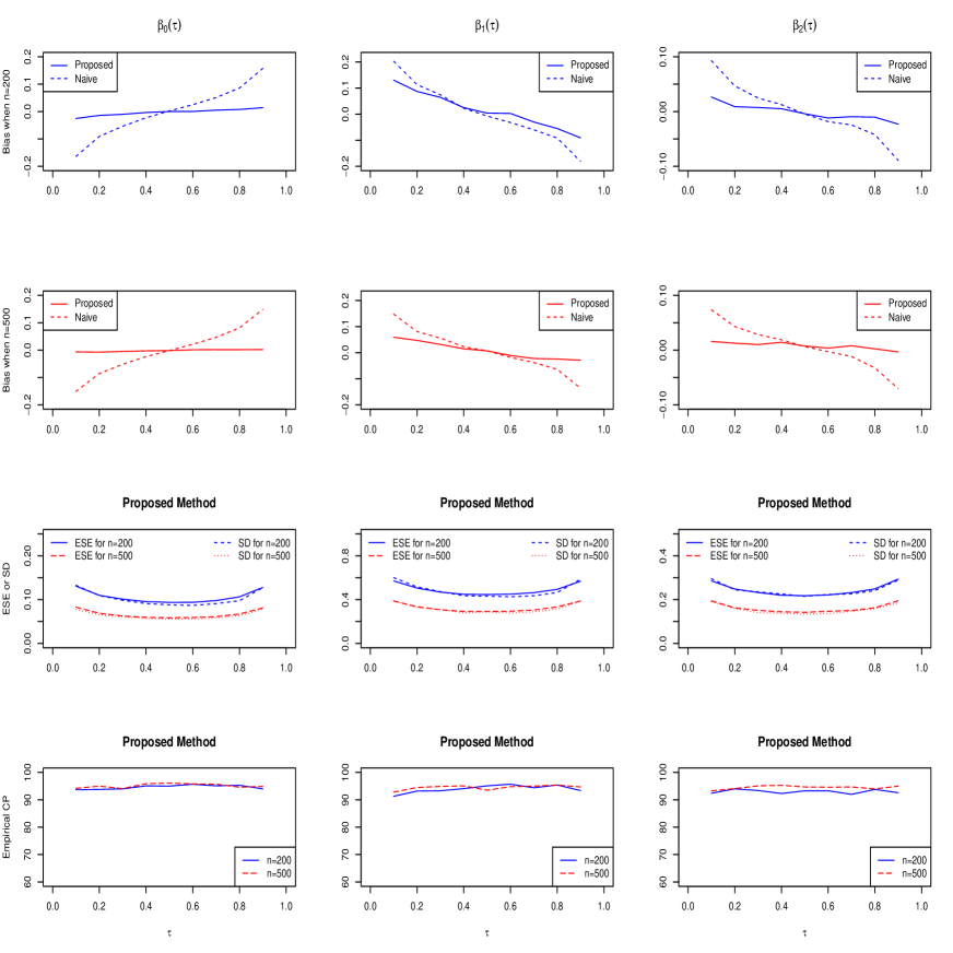
Figure 2: Simulation results for Case 1. Lines in blue correspond to the results with $n=200$ and lines in red correspond to the results with $n=500$. ESE stands for the estimated standard error, SD stands for the empirical standard deviation, and CP stands for the coverage probability of a 95% confidence interval.

We further examine the robustness of our approach to the misspecification of the trajectory error distribution. Specifically, we generate the $\epsilon_{ij}$ from the uniform distribution $Unif(-\sqrt{3}/2,\sqrt{3}/2)$, while applying $\hat{\boldsymbol{\beta}}(\tau)$ that assumes the Laplace or Normal trajectory errors. The simulation results are given in Figure 3. We observe through comparing Figure 3 and Figure 2 that the estimator that does not assume the correct trajectory error distribution (Uniform versus Laplace) only yields slight elevated estimation bias. Given the sample size $n=500$, the empirical bias seems quite negligible. The impact of misspecifying the error distribution on the variance estimation and coverage probabilities is also minimal, particularly for the larger sample size. These results demonstrate the robust performance of the proposed estimator.

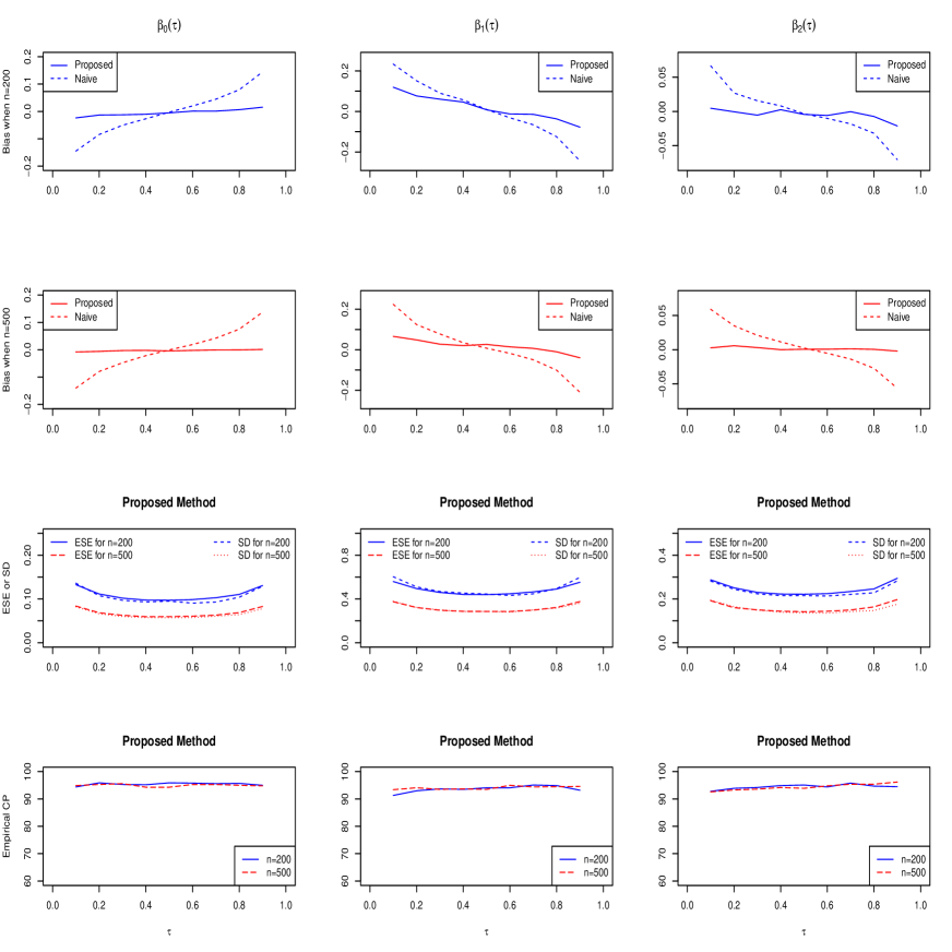
Figure 3: Simulation results for the robustness study. Lines in blue correspond to the results with $n=200$ and lines in red correspond to the results with $n=500$. ESE stands for the estimated standard error, SD stands for the empirical standard deviation, and CP stands for the coverage probability of a 95% confidence interval.

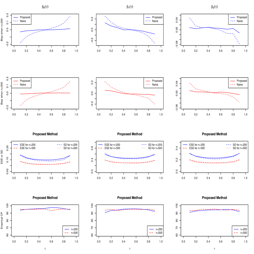
Figure 4: Simulation results for quadratic trajectory model with Laplace errors. Lines in blue correspond to the results with $n=200$ and lines in red correspond to the results with $n=500$. ESE stands for the estimated standard error, SD stands for the empirical standard deviation, and CP stands for the coverage probability of a 95% confidence interval.

In addition, we consider a setting where the longitudinal trajectory model is not linear over time, as often encountered in practice. Specifically, the longitudinal observations are generated from the following model:

$$Y_{ij}=a_{i}+b_{i}t_{ij}+c_{i}t_{ij}^{2}+\epsilon_{ij}/(1+X_{1i}),~{}~{}~{}~{}~{}~{}~{}~{}j=1,\ldots,m_{i};~{}i=1,\ldots,n,$$

and the trajectory feature is the changing rate of $Y_{i}(t)$ at a given time point $t_{*}$, i.e. $B_{i}=b_{i}+2c_{i}t_{*}=2+X_{1i}+X_{2i}+(0.1+X_{1i}+X_{2i})e_{i}$. Here we let $a_{i}\sim\mbox{Exp}(0.15)$, $c_{i}\sim\mbox{Exp}(0.15)$, and $t_{*}=1$. We generate $t_{ij}$, $\boldsymbol{X}_{i}$ and $e_{i}$ in the same way as before. The results when $\epsilon_{ij}$ follows from the Laplace distribution are plotted in Figures 4; see the Supplementary Materials for the other results correspond to the normal error distribution. Similar to Figure 2, Figure 4 suggests substantial bias reduction resulted from the proposed method as compared to the naive ones. The coverage probabilities match quite well with the nominal value especially when $n=500$. The empirical standard errors and the estimated ones agree well and decrease with the sample size as expected. Overall, the performance of the proposed method are comparable between the cases with nonlinear and linear trajectory models.

6 Analysis of the DURABLE Study

Diabetes is a chronic disease in which there are high blood sugar levels over a prolonged period. It is a major cause of blindness, kidney failure, heart attacks, stroke and lower limb amputation and is the 7th leading cause of death affecting 422 million people worldwide (Roglic et al., 2016). Insulins are important treatments for diabetes. The DURABLE Buse et al. (2009) trial was designed to study the efficacy, safety, and durability of two common insulin initiation regimens: twice-daily insulin lispro mixture 75/25 (LM75/25) versus once-daily insulin glargine (GL) added to oral antihyperglycemic drugs (OADs) to achieve and maintain hemoglobin A1c (HbA1c) goals. This randomized, open label, parallel study enrolled 2187 insulin-naive patients with type 2 diabetes from 11 countries, aged 30 to 80 years, with HbA1c $>7.0\%$ on at least two oral antihyperglycemic agents. The HbA1c level was collected every 6 weeks during 24 weeks.

HbA1c level is an important index of glycemic control. To assess the efficacy of different treatments, we analyze the longitudinal measurements of HbA1c under the proposed quantile regression framework. Specifically, let $Y_{ij}$ represent the $j$-th HbA1c measurements of the $i$th individual recorded in the $t_{ij}$th week since the study enrollment ($j=1,\ldots,m_{i}$). After examining the observed data, we assume a quadratic trajectory model for within-subject HbA1c measurements during the 24 week follow-up period. That is,

$$Y_{ij}=\alpha_{i0}+\alpha_{i1}t_{ij}+\alpha_{i2}t_{ij}^{2}+\epsilon_{ij}.$$

Under this model, the random intercept $\alpha_{i0}$ denotes the subject-specific baseline HbA1c measurement, and the subject-specific decreasing rate of HbA1c at a specified time point $t^{*}$ is given by $-\alpha_{i1}-2\alpha_{i2}t^{*}$. In our analysis, we take $t^{*}=3$ (corresponding to 12 weeks) and set $B_{i}\doteq-\alpha_{i1}-2\alpha_{i2}t^{*}$, a meaningful trajectory feature which is not directly observed. Under this setup, we exploit how treatments and other risk factors influence the HbA1c reduction rate at 12 weeks after the initiation of the assigned insulin treatment. By adopting the quantile regression modeling, we can further delineate whether and how their associations with $B_{i}$ vary across diabetes patients.

The covariate of our main interest is therapy, coded as 1 if the subject took the LM75/25 regimen and 0 if GL regimen. We consider three other covariates according to our exploratory analysis: sulfouse, 1 if the subject uses the sulfonylurea (SU) and 0 otherwise; basfglu, baseline fasting plasma glucose; and basfins, baseline fasting insulin. Here we standardize basfglu and basfins by subtracting their means and then dividing by their standard deviations. Because the two regimes are added to OADs, we also include the interaction term, therapy$*$sulfouse, in our model to examine if the treatment effect (i.e. LM75/25 versus GL) on the HbA1c decreasing rate is modified by the use of SU. We exclude 107 subjects who have missing covariates in the analysis. We also exclude 263 subjects who have less than three measurements of HbA1c, because they do not contribute information to studying $B_{i}$. There are 1,717 subjects in our analysis; 71 subjects are in GL group without SU, 800 subjects are in GL group with SU, 65 subjects are in LM75/25 group without SU, and 781 subjects are in LM75/25 group with SU. The continuous covariate basfglu ranges from 1.04 to 26, with mean=11 and standard deviation=3.6. The basfins ranges from $-2$ to 143, with mean=10 and standard deviation=9.0.

We apply the proposed method to perform quantile regression for $B_{i}$ on the covariates specified above at quantile levels equally spaced between $0.1$ and $0.8$ with step size $0.02$. For selecting the smoothing parameter $h$, we employ the procedure introduced in Subsection 3.4 on a $h$-grid between $0.8$ and $1.5$ with step size 0.1. In Fig. 5, we plot the proposed estimated coefficients (red solid line) along with the 95% pointwise confidence intervals (red dot dashed lines) for $\tau\in[0.1,0.8]$ based on 200 resampling samples. The naive estimators (black dashed lines) are also plotted for comparisons. In Fig. 5, the estimated intercept coefficients represent the estimated quantiles of HbA1c decreasing rate for subjects receiving GL therapy, no SU use, with baseline fasting glucose and baseline fasting insulin set as 10.98mmol/L and 10.06 units (which are their observed average values in this dataset). For example, Fig. 5 shows that the estimated median rate of HbA1c decreasing is about 0.34 (%) per month. Compared to the naive estimates, the proposed estimates are generally less jagged (over $\tau$) and have narrower confidence intervals. Some naive estimates even lie outside the proposed confidence intervals. These observations indicate the benefits of applying the proposed method over the naive approach.

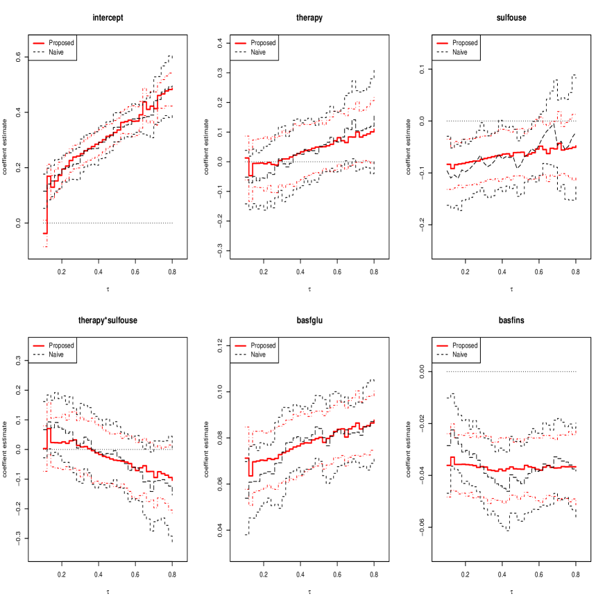
Figure 5: The DURABLE data example: the proposed coefficient estimates (red solid line) and the 95% pointwise confidence intervals (red dot-dashed line), the naive coefficient estimates (black long-dashed line) and 95% pointwise confidence intervals (black dashed line)

To interpret the covariate coefficients in Figure 5, note that positive covariate coefficients indicate quicker HbA1c decreasing over time given one unit increase in the corresponding covariate. We observe that the coefficients for baseline fasting glucose and baseline fasting insulin are significantly different from 0 for all $\tau$’s considered. These results suggest that a higher baseline fasting glucose and a lower baseline fasting insulin are significantly associated faster decreasing of HbA1c. These are sensible findings that can explained as follows. First, a higher baseline glucose generally implicates a higher baseline HbA1c. It is reasonable to expect a more rapid HbA1c reduction for those with high baseline HbA1c values compared to those with low baseline HbA1c values. Secondly, a lower baseline insulin may imply less insulin resistance. Consequently, it is associated with a stronger response to an insulin treatment that is manifested by a quicker HbA1c decreasing.

To evaluate the treatment effect, we examine the coefficient plots for therapy, sulfuse, and therapy*sulfuse simultaneously. In the presence of the interaction term therapy*sulfuse, the coefficients for therapy can be interpreted as the treatment effect for subjects without SU use. The estimated coefficients for therapy suggest that the therapy LM75/25 may offer some significant advantage over GL in terms of lowering HbA1c more quickly among the “strong” responders of the insulin treatments (corresponding to the large $\tau$’s) when SU is not used. For the subjects with sustained HbA1c, either due to low baseline HbA1c or weak response to the insulin treatment, the GL and LM75/25 therapies demonstrate little difference in the decreasing rate of HbA1c. The estimated coefficients for sulfuse suggest some negative impact of using SU on the treatment efficacy in lowering HbA1c. The negative impact seems diminished in “strong” responders of the insulin treatment.

In Fig. 6, we plot the estimates for therapy coefficient $+$ therapy*sulfouse coefficient and sulfouse coefficient $+$ therapy*sulfouse coefficient, which represent the treatment effect for subjects with SU use and the effect of SU use for subjects receiving LM75/25. Comparing Fig. 6 with the plots for therapy and sulfuse in Fig. 5, we see that for subjects with SU, choosing LM75/25 versus GL has little impact on the HbA1c decreasing rate, while LM75/25 demonstrates some moderate advantage over GL for subjects without SU use. This may be due to the fact that SU is a treatment for lowering postprandial blood glucose level, GL is a basal insulin to lower the overall glucose level, and LM75/25 targets both basal and postprandial. Therefore, when SU is added, both GL and LM75/25 will cover basal and postprandial blood glucose, thereby resulting in similar glycemic control, and hence similar HbA1c decreasing rates. Without SU, LM75/25 can cover postprandial glucose, while GL cannot; therefore LM75/25 demonstrates some moderate benefit over GL. It is also shown by comparing Fig. 6 with Fig. 5 that for subjects treated with LM75/25, using SU may be associated with slower HbA1c reduction; its effect has a consistent direction with but a smaller magnitude than that in subjects treated with GL, particularly for $\tau$’s less than $0.5$. The overall negative impact of SU may associate with hypoglycemic events, as SU is a known significant factor to cause hypoglycemic events, which limits titrating insulin (Fu et al., 2014) and then lead to worse glycemic control. The smaller impact of SU use under LM75/25 (versus that under GL) may be explained by the bigger overlap in glucose control coverage between SU and LM75/25. Despite these sensible observations regarding the interaction between therapy and sulfouse, the confidence intervals for the coefficient for therapy*sulfouse (see Fig. 5) do not suggest statistical significance. This is likely due to the small size of the group without SU use. A larger future study may help provide a more confirmative conclusion.

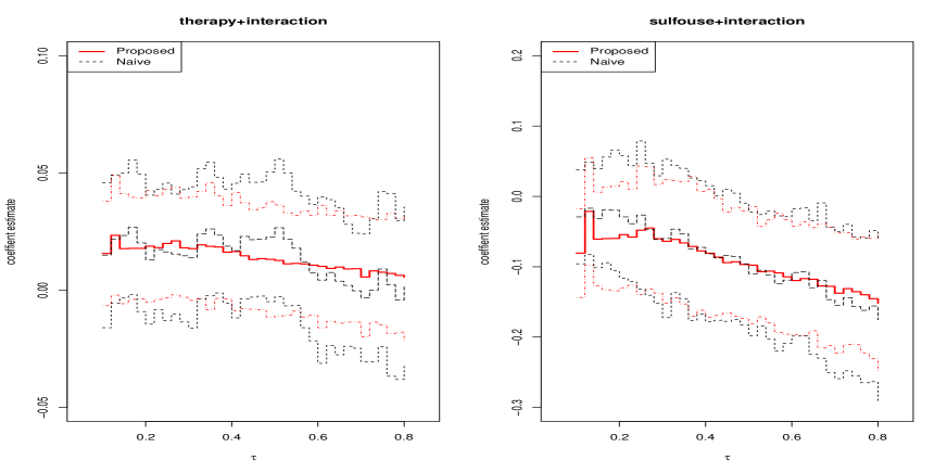
Figure 6: The DURABLE data example: the estimates for therapy coefficient plus therapy*sulfouse coefficient and sulfouse coefficient plus therapy*sulfouse coefficient, and the corresponding 95% pointwise confidence intervals. Red lines correspond to the proposed method and black lines correspond to the naive method.

Finally, we employ the proposed test $\mathcal{T}$ to assess whether or not the effects of therapy and other covariates are constant over $\tau$. We set $\tau_{L}=0.1$ and $\tau_{U}=0.8$ and adopt $\Xi(v)=I\{v>(\tau_{L}+\tau_{U})/2\}$. For the coefficient for therapy, we obtain $\mathcal{T}=0.589$, which falls into the rejection region $(-\infty,-0.259)\cup(0.291,\infty)$ at level $0.05$. This suggests that the difference between LM75/25 and GL may vary across type II diabetes patients. For example, it may differ by the status of SU use as suggested by Fig. 5 and Fig. 6. We also reject the constancy of the effect of basfglu. This is consistent with our observation in Fig. 5, which is, baseline fasting glucose has a bigger influence on the upper quantiles of the HbA1c decreasing rate. Our constancy tests suggest that the location-shift effects may be adequate for sulfouse and basfins.

It is worth mentioning that we also apply the proposed method assuming the linear trajectory model for within-subject HbA1c. We obtain quite similar results regarding the covariate effects on the decreasing rate of HbA1c at the $12$ weeks follow-up. The counterparts of Fig. 5 and Fig. 6 are presented in the Supplementary Materials; see Figures S5 and S6. This suggests the robustness of the proposed trajectory quantile regression method to the specification of the underlying trajectory model.

7 Discussion

This work, to the best of our knowledge, is the first effort to utilize the device of quantile regression to explore the associates of longitudinal outcome trajectory which may follow heterogeneous patterns. As a proof of concept, we assume polynomial outcome trajectories in the present paper, while the methodology can readily be extended to accommodate nonparametric trajectories, for example, through B-Spline. The details with such extensions will be spelled out in separate work.

In this paper, we derive the regression quantiles of the latent trajectory feature when the error term in the trajectory model follows the Normal or Laplace distribution. Appealingly, they take the same practical form, as pointed out at the end of Section 3.2, and are shown to have robust performance when the trajectory errors follow a different distribution. It is worth noting that the bias correction strategy adopted in the proposed estimation procedure can be further extended to a wider class of distribution families, as long as their characteristic functions are proportional to the inverse of a polynomial; see Hong and Tamer (2003) and Wang et al. (2012) for related discussions. This entails broader applicability and enhanced usefulness of the proposed trajectory quantile regression framework.

Supplementary Materials

Supplementary Materials, which include large sample properties, justification of the proposed resampling-based inference procedure, additional simulation studies, and linear trajectory model for DURABLE data are available online.

Acknowledgements

This work was partially supported by National Institutes of Health Grants R01HL113548.

References

- Buse et al. (2009) Buse, J., Wolffenbuttel, B., Herman, W., Shemonsky, N., Jiang, H., Fahrbach, J., Scism-Bacon, J., and Martin, S. (2009). Durability of basal versus lispro mix 75/25 insulin efficacy (durable) trial 24-week results: safety and efficacy of insulin lispro mix 75/25 versus insulin glargine added to oral antihyperglycemic drugs in patients with type 2 diabetes. Diabetes Care 32, 1007–1013.
- Carroll et al. (2006) Carroll, R., Ruppert, D., Stefanski, L., and Crainiceanu, C. (2006). Measurement Error in Nonlinear Models: A Modern Perspective. Chapman & Hall, London.
- Chen et al. (2004) Chen, L., Wei, L., and Parzen, M. (2004). Quantile regression for correlated observations. Proceedings of the Second Seattle Symposium in Biostatistics 179, 51–69.
- Delaigle and Hall (2008) Delaigle, A. and Hall, P. (2008). Using simex for smoothing-parameter choice in errors-in-variables problems. Journal of the American Statistical Association 103, 280–287.
- Diggle et al. (2002) Diggle, P., Heagerty, P., Liang, K.-Y., and Zeger, S. (2002). Analysis of Longitudinal Data (second edition). Oxford University Press, Oxford.
- Fitzmaurice et al. (2004) Fitzmaurice, G., Laird, N., and Ware, J. (2004). Applied Longitudinal Analysis. Wiley-Interscience, Hoboken, NJ.
- Fu et al. (2015) Fu, H., Cao, D., Boye, K., Curtis, B., Schuster, D., Kendall, D., and Ascher-Svanum, H. (2015). Early glycemic response predicts achievement of subsequent treatment targets in the treatment of type 2 diabetes: A post hoc analysis. Diabetes Therapy 6, 317–328.
- Fu et al. (2014) Fu, H., Xie, W., Curtis, B., and Schuster, D. (2014). Identifying factors associated with hypoglycemia-related hospitalizations among elderly patients with t2dm in the us: a novel approach using influential variable analysis. Current Medical Research and Opinion 30, 1787–1793.
- Fu and Wang (2012) Fu, L. and Wang, Y. (2012). Quantile regression for longitudinal data with a working correlation model. Computational Statistics and Data Analysis 56, 2526–2538.
- Galvao (2011) Galvao, A. (2011). Quantile regression for dynamic panel data with fixed effects. Journal of Econometrics 164, 142–157.
- Galvao and Montes-Rojas (2010) Galvao, A. and Montes-Rojas, G. (2010). Penalized quantile regression for dynamic panel data. Journal of Statistical Planning and Inference 140, 3476–3497.
- Hand and Crowder (1996) Hand, D. and Crowder, M. (1996). Practical Longitudinal Data Analysis. Chapman & Hall, London.
- Harding and Lamarche (2009) Harding, M. and Lamarche, C. (2009). A quantile regression approach for estimating panel data models using instrumental variables. Economics Letters 104, 133–135.
- He et al. (2003) He, X., Fu, B., and Fung, W. (2003). Median regression for longitudinal data. Statistics in Medicine 22, 3655–3669.
- He and Liang (2000) He, X. and Liang, H. (2000). Quantile regression estimates for a class of linear and partially linear errors-in-variables models. Statistica Sinica 10, 129–140.
- Hedeker (2006) Hedeker, D. (2006). Longitudinal data analysis. Wiley-Interscience, Hoboken, N.J.
- Hong and Tamer (2003) Hong, H. and Tamer, E. (2003). A simple estimator for nonlinear error in variable models. Journal of Econometrics 117, 1–19.
- Horowitz (1998) Horowitz, J. (1998). Bootstrap methods for median regression models. Econometrica 66, 1327–1351.
- Jin et al. (2001) Jin, Z., Ying, Z., and Wei, L. (2001). A simple resampling method by perturbing the minimand. Biometrika 88, 381–390.
- Jones (1993) Jones, R. (1993). Longitudinal Data With Serial Correlation: A State-space Approach. Chapman & Hall, London.
- Jung (1996) Jung, S.-H. (1996). Quasi-likelihood for median regression models. Journal of the American Statistical Association 91, 251–257.
- Koenker (2004) Koenker, R. (2004). Quantile regression for longitudinal data. Journal of Multivariate Analysis 91, 74–89.
- Koenker (2005) Koenker, R. (2005). Quantile Regression. Cambridge University Press, New York.
- Koenker and Bassett (1978) Koenker, R. and Bassett, G. (1978). Regression quantiles. Econometrica 46, 33–50.
- Kotz et al. (2001) Kotz, S., Kozubowski, T., and Podgorski, K. (2001). The Laplace Distribution and Generalizations. Birkhauser, Boston.
- Lee and Kong (2013) Lee, M. and Kong, L. (2013). Quantile regression for longitudinal biomarker data subject to left censoring and dropouts. Communications in Statistics - Theory and Methods .
- Leng and Zhang (2014) Leng, C. and Zhang, W. (2014). Smoothing combined estimating equations in quantile regression for longitudinal data. Statistics and Computing 24, 123–136.
- Liang and Zeger (1986) Liang, K.-Y. and Zeger, S. (1986). Longitudinal data analysis using generalized linear models. Biometrika 73, 13–22.
- Lipsitz et al. (1997) Lipsitz, S. R., Fitzmaurice, G. M., Molenberghs, G., and Zhao, L. P. (1997). Quantile regression methods for longitudinal data with drop-outs: application to cd4 cell counts of patients infected with the human immunodeficiency virus. Journal of the Royal Statistical Society: Series C (Applied Statistics) 46, 463–476.
- Lu and Fan (2015) Lu, X. and Fan, Z. (2015). Weighted quantile regression for longitudinal data. Computational Statistics 30, 569–592.
- Nakamura (1990) Nakamura, T. (1990). Corrected score function for errors-in-variables models: methodology and application to generalized linear models. Biometrika 77, 127–137.
- Peng and Fine (2009) Peng, L. and Fine, J. (2009). Competing risks quantile regression. Journal of the American Statistical Association 104, 1440–1453.
- Raudenbush and Bryk (2002) Raudenbush, S. W. and Bryk, A. S. (2002). Hierarchical linear models : applications and data analysis methods. Sage Publications, 2nd Ed., Thousand Oaks, CA.
- Roglic et al. (2016) Roglic, G. et al. (2016). Who global report on diabetes: A summary. International Journal of Noncommunicable Diseases 1, 3.
- Snijders and Bosker (2002) Snijders, T. A. and Bosker, R. J. (2002). Multilevel analysis : an introduction to basic and advanced multilevel modeling (Reprint. ed.). Sage Publications, London.
- Stefanski (1989) Stefanski, L. (1989). Unbiased estimation of a nonlinear function of a normal-mean with application to measurement error models. Communications in Statistics–Theory and Methods 18, 4335–4358.
- Stefanski and Carroll (1985) Stefanski, L. and Carroll, R. (1985). Covariate measurement error in logistic regression. The Annals of Statistics 13, 1335–1351.
- Stefanski and Carroll (1987) Stefanski, L. and Carroll, R. (1987). Conditional scores and optimal scores for generalized linear measurement-error models. Biometrika 74, 703–716.
- Stefanski and Carroll (1990) Stefanski, L. and Carroll, R. (1990). Deconvolunting kernel density estimators. Statistics 21, 165–184.
- Stefanski and Cook (1995) Stefanski, L. and Cook, J. (1995). Simulation-extrapolation: the measurement error jackknife. Journal of the American Statistical Association 90, 1247–1256.
- Sun et al. (2016) Sun, X., Peng, L., Manatunga, A., and Marcus, M. (2016). Quantile regression analysis of censored longitudinal data with irregular outcome-dependent follow-up. Biometrics 72, 64–73.
- Sun et al. (2007) Sun, Y., Zhang, W., and Tong, H. (2007). Estimation of the covariate matrix of random effects in longitudinal studies. The Annals of Statistics pages 2795–2814.
- Verbeke and Molenberghs (2000) Verbeke, G. and Molenberghs, G. (2000). Linear Mixed Models for Longitudinal Data. Springer-Verlag, New York.
- Wang and Fygenson (2009) Wang, H. and Fygenson, M. (2009). Inference for censored quantile regression models in longitudinal studies. The Annals of Statistics 37, 756–781.
- Wang et al. (2012) Wang, H., Stefanski, L., and Zhu, Z. (2012). Corrected–loss estimation for quantile regression with covariate measurement error. Biometrika 99, 405–421.
- Wei and Carroll (2009) Wei, Y. and Carroll, R. (2009). Quantile regression with measurement errors. Journal of the American Statistical Association 104, 1129–1143.
- Wu et al. (2015) Wu, Y., Ma, Y., and Yin, G. (2015). Smoothed and corrected score approach to censored quantile regression with measurement errors. Journal of the American Statistical Association 110, 1670–1683.