A new and finite family of solutions of hydrodynamics
Part I: Fits to pseudorapidity distributions

Abstract

We highlight some of the interesting properties of a new and finite, exact family of solutions of 1 + 1 dimensional perfect fluid relativistic hydrodynamics. After reviewing the main properties of this family of solutions, we present the formulas that connect it to the measured rapidity and pseudo-rapidity densities and illustrate the results with fits to p+p collisions at 8 TeV and Pb+Pb collisions at $\sqrt{s_{NN}}=5.02$ TeV.

1 Introduction

In this manuscript we discuss a new family of exact solutions of perfect fluid hydrodynamics for a 1+1 dimensional, longitudinally expanding fireball. The applications of 1+1 dimensional hydrodynamics to particle production in high energy physics has a long and illustrous history, that include some of the most renowned theoretical papers in high energy heavy ion physics.

In high energy collisions, thermal models to describe particle production rates were introduced by Fermi in 1950  [1]. It was soon pointed out by Landau, Khalatnikov and Belenkij  [2, 3, 4], that the momentum spectrum can also be explained in these collisions if one assumes not only global but also local thermal equilibrium. Landau and collaborators predicted [4], that perfect fluid hydrodynamical modelling will be a relevant tool for the analysis of experimental data of strongly interacting high energy collisions. After 60 years, this field is still interesting and surprizing, as reviewed recently in ref. [5]. Applications of exact solutions of relativistic hydrodynamics to describe pseudo-rapidity distributions in high energy collisions were reviewed recently in ref. [6].

2 Equations of relativistic hydrodynamics

Relativistic perfect fluids are locally thermalized fluids, their dynamical equations of motion correspond to the local conservation of the flow of entropy and the flow of four momentum:

$$\partial_{\mu}\left(\sigma u^{\mu}\right) = 0,$$ (1)

$$\partial_{\nu}T^{\mu\nu} = 0,$$ (2)

where the entropy density is denoted by $\sigma=\sigma(x)$, four velocity is $u^{\mu}$, normalized as $u^{\mu}u_{\mu}=1$, and the energy-momentum four tensor is denoted by $T^{\mu\nu}$. These fields are functions of the four coordinate $x^{\mu}=(t,\mathbf{r})=\left(t,r_{x},r_{y},r_{z}\right)$. Similarly, the four momentum is denoted by $p^{\mu}=(E_{p},\mathbf{p})=\left(E_{p},p_{x},p_{y},p_{z}\right)$, where the energy is on mass-shell, $E_{p}=\sqrt{m^{2}+\mathbf{p}^{2}}$, where the mass of the observed type of particle is indicated by $m$.

The energy-momentum four tensor $T^{\mu\nu}$ of a perfect fluid is given as

$$T^{\mu\nu}=\left(\varepsilon+p\right)u^{\mu}u^{\nu}-pg^{\mu\nu},$$ (3)

where the metric tensor is $g^{\mu\nu}=\textnormal{diag}(1,-1,-1,-1)$, the energy density is indicated by $\varepsilon$ and the pressure by $p$.

The five dynamical equations of relativistic hydrodynamics connect six variables, the entropy, the energy density, the pressure and the three spatial components of the four velocity $u^{\mu}=\gamma(1,\mathbf{v})$. This set of equations is closed by the equation of state, that characterizes the properties of the flowing matter. We assume, that this is given by

$$\varepsilon=\kappa p,$$ (4)

where in this paper, $\kappa$ is assumed to be a constant, independent of the temperature $T$. For net baryon free matter, the baryochemical potential is $\mu_{B}=0$, hence the fundamental thermodynamical relation reads as $\varepsilon+p=T\sigma$, so the temperature field can also be chosen as one of the local characteristics of the matter.

In this paper we recapitulate a recent solution of relativistic hydrodynamics in $1$$+$$1$ dimensions, with a realistic speed of sound

$$c_{s}=\sqrt{\left.\frac{\partial\varepsilon}{\partial p}\right|_{\sigma}}\,=\,1/\sqrt{\kappa},$$ (5)

where in the calculations we use the average value of the speed of sound, $c_{s}=0.35\pm 0.05$ as measured by the PHENIX Collaboration in $\sqrt{s_{NN}}=200$ GeV Au+Au collisions in ref. [7].

3 The CKCJ solution

In $1$$+$$1$ dimensions, it is useful to rewrite the equations of relativistic hydrodynamics in Rindler coordinates $(\tau,\eta_{x})$  [10, 11, 12, 6]. The (longitudinal) proper-time $\tau$ and the coordinate-space rapidity $\eta_{x}$ are

$$\left(\tau,\eta_{x}\right)=\left(\,\sqrt{t^{2}-r_{z}^{2}}\,,\frac{1}{2}\textnormal{ln}\left[\frac{t+r_{z}}{t-r_{z}}\right]\,\right),$$ (6)

while the fluid rapidity $\Omega$$=$$\frac{1}{2}\textnormal{ln}\left(\frac{1+v_{z}}{1-v_{z}}\right)$ relates to the four and to the three velocity as $u^{\mu}$$=$ $\left(\cosh\left(\Omega\right),\sinh\left(\Omega\right)\right)$, $v_{z}$$=$$\tanh\left(\Omega\right)$.

A finite and accelerating, realistic 1+1 dimensional solution of relativistic hydrodynamics was recently given by Csörgő, Kasza, Csanád and Jiang (CKCJ)  [6] as a family of parametric curves:

$$\eta_{x}(H) = \Omega(H)-H,$$ (7)

$$\Omega(H) = \frac{\lambda}{\sqrt{\lambda-1}\sqrt{\kappa-\lambda}}\textnormal{arctan}\left(\sqrt{\frac{\kappa-\lambda}{\lambda-1}}\textnormal{tanh}\left(H\right)\right),$$ (8)

$$\sigma(\tau,H) = \sigma_{0}\left(\frac{\tau_{0}}{\tau}\right)^{\lambda}\mathcal{V}_{\sigma}(s)\left[1+\frac{\kappa-1}{\lambda-1}\textnormal{sinh}^{2}(H)\right]^{-\frac{\lambda}{2}},$$ (9)

$$T(\tau,H) = T_{0}\left(\frac{\tau_{0}}{\tau}\right)^{\frac{\lambda}{\kappa}}\mathcal{T}(s)\left[1+\frac{\kappa-1}{\lambda-1}\textnormal{sinh}^{2}(H)\right]^{-\frac{\lambda}{2\kappa}},$$ (10)

$$\mathcal{T}(s) = \frac{1}{\mathcal{V}_{\sigma}(s)},$$ (11)

$$s(\tau,H) = \left(\frac{\tau_{0}}{\tau}\right)^{\lambda-1}\textnormal{sinh}(H)\left[1+\frac{\kappa-1}{\lambda-1}\textnormal{sinh}^{2}(H)\right]^{-\lambda/2},$$ (12)

where the parameter of the solutions, denoted by $H$, stands also for the difference between the fluid rapidity $\Omega$ and the space-time rapidity $\eta_{x}$. Near mid-rapidity, these solutions are approximately, but not exactly self-similar [6], they depend on the space-time rapidity $\eta_{x}$ predominantly through the scaling functions $\mathcal{T}(s)$ and $\mathcal{V}_{\sigma}(s)$, that in turn depend on the scaling variable $s$. The solutions for the fields $F$$=$$\left\{\sigma,T,\Omega\right\}$, and the scaling variable $s$ are given with explicit dependence on the longitudinal proper-time $\tau$ and as parametric solutions in terms the parameter $H$. Any of the above space-time dependent field can be visualized as parametric (hyper)surfaces:

$$\left(t,r_{z},F(t,r_{z})\right)=\left(\tau\cosh(\eta_{x}(H)),\,\tau\sinh(\eta_{x}(H)),\,F_{s}(\tau,H)\right),$$ (13)

where the subscript $s$ indicates that this function is to be taken from the parametric solutions, eqs. (7-12), as a function of $\tau$ and $H$. The functional form of such a bi-variate function $F_{s}(\tau,H)$, depends on its variables differently from the functional form of the also bi-variate function $F(t,r_{z})$, as usual.

This new, longitudinally finite family of solutions is illustrated by Fig. 1, for a realistic value of the speed of sound, $c_{s}^{2}=1/\kappa=0.1$ and for a realistic value of the acceleration parameter, $\lambda=1.14$. This figure shows clearly, that the CKCJ solution is limited to a cone within the forward light-cone around mid-rapidity. The formulas that give the limiting values of the space-time rapidity are determined from the requirement that the parametric curves of the solution correspond to functions, as detailed in ref. [6].

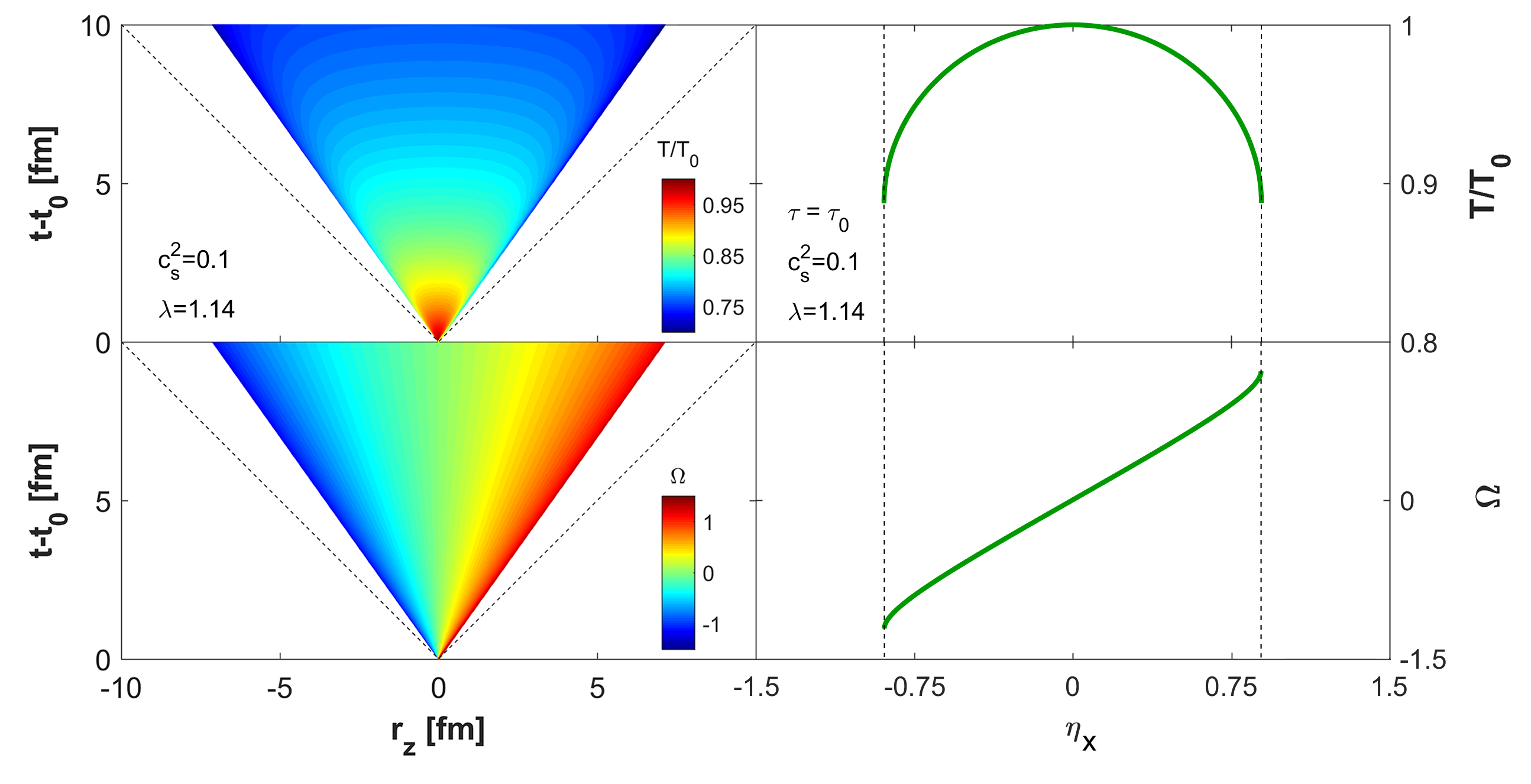
Figure 1: Illustration of a CKCJ exact solution [6] of relativistic hydrodynamics. The top left panel shows the space-time evolution of the temperature distribution, $T(t,r_{z})$, while the bottom left panel shows the same for the fluid rapidity distribution, $\Omega(t,r_{z})$. The top right panel shows the temperature at a constant value of the longitudinal proper time $\tau$, as a function of the space-time rapidity $\eta_{x}$, where the dashed vertical lines indicate the lower and upper limits of the applicability of the CKCJ solution. The bottom right panel is the same, but it indicates $\Omega(\eta_{x})$ which in this class of solutions is independent of the longitudinal proper time $\tau$.

4 Rapidity and pseudo-rapidity distributions

Let us clarify first the definition of the observables of the single-particle spectrum in momentum-space. The pseudorapidity $\eta_{p}$ and the rapidity $y$ of a final state particle with mass $m$ and four momentum $p^{\mu}$ are defined as $\eta_{p}$$=$$\frac{1}{2}\ln\left(\frac{p+p_{z}}{p-p_{z}}\right)$ and $y$$=$$\frac{1}{2}\textnormal{ln}\left(\frac{E+p_{z}}{E-p_{z}}\right),$ where the modulus of the three-momentum is $p=|\mathbf{p}|=\sqrt{p_{x}^{2}+p_{y}^{2}+p_{z}^{2}}$.

The rapidity and the pseudorapidity distributions were derived from the CKCJ solutions in ref. [6], as follows. As a first step, these 1+1 dimensional solutions were embbedded to the 1+3 dimensional space. Subsequently we assumed, that the freeze-out hypersurface is pseudo-orthogonal to the four velocity and utilized advanced saddle-point integration methods, to obtain an analytic expression for the rapidity density distribution [6]:

$$\frac{dn}{dy}\approx\left.\frac{dn}{dy}\right|_{y=0}\cosh^{-\frac{1}{2}\alpha(\kappa)-1}\left(\frac{y}{\alpha(1)}\right)\exp\left(-\frac{m}{T_{\rm eff}}\left[\cosh^{\alpha(\kappa)}\left(\frac{y}{\alpha(1)}\right)-1\right]\right),$$ (14)

where $\alpha(\kappa)$ is defined as $\alpha(\kappa)$$=$$\frac{2\lambda-\kappa}{\lambda-\kappa}$. The mass of the particle $m$ is the mass of the identified particles (typically pions). The above formula depends on four fit parameters, $\kappa$, $\lambda$, $T_{\rm eff}$ and $\left.\frac{dn}{dy}\right|_{y=0}$. These relate to the speed of sound, the acceleration, the effective temperature (that corresponds to the slope parameter of the invariant transverse mass spectrum at mid-rapidity), and the value of the rapidity density at mid-rapidity. The values of $T_{\rm eff}$ should be determined from fits to the transverse mass spectra of hadrons, and while $\kappa$ determines the average value of the speed of sound, measured for example in ref. [7]. The two key parameters of the rapidity density distributions are thus the acceleration parameter $\lambda$, and the midrapidity density, which is just an overall normalization factor. Thus the shape of the rapidity distributions is controlled predominantly by the acceleration parameter $\lambda$. Both $\left.\frac{dn}{dy}\right|_{y=0}$ and $\lambda$ can be extraced from fits to experimental data. As the measurement of the rapidity density distributions requires particle identification, the pseudorapidity densities are more readily determined.

Using similar methods, the pseudorapidity density distribution was determined as a parametric curve, where the parameter of the curve is the momentum-space rapidity $y$:

$$\left(\eta_{p}(y)\,,\frac{dn}{d\eta_{p}}(y)\right)=\left(\frac{1}{2}\log\left[\frac{\bar{p}(y)+\bar{p}_{z}(y)}{\bar{p}(y)-\bar{p}_{z}(y)}\right]\,,\frac{\bar{p}(y)}{\bar{E}(y)}\frac{dn}{dy}\right),$$ (15)

where $\bar{A}(y)$ denotes the rapidity dependent average value of the variable $A$, representing various components of the four momentum. The Jacobian connecting the double differential ($y$, $m_{t}$) and ($\eta_{p}$, $m_{t}$) distributions has been utilized at the average value of the transverse momentum, following ref. [10]. In contrast to earlier results, a new element is that this CKCJ solution gives an explicit relation between the $\bar{p}_{T}(y)$, the rapidity dependent average transverse momentum, the slope parameter at mid-rapidity $T_{\rm eff}$ and the mass of the observed particles $m$ as follows:

$$\bar{p}_{T}(y)\approx{\sqrt{T_{\rm eff}^{2}+2mT_{\rm eff}}}\left(1+\frac{\alpha(\kappa)}{2\alpha(1)^{2}}\frac{T_{\rm eff}+m}{T_{\rm eff}+2m}y^{2}\right)^{-1}.$$ (16)

Note, that the same functional form, a Lorentzian shape was obtained for the rapidity dependence of the slope of the transverse momentum spectrum in the Buda-Lund hydro model of ref. [15]. The coefficient of the $y^{2}$ dependent term was considered as a free fit parameter even very recently, in refs. [16, 17]. This coefficient is now expressed with the help of $\kappa$, the parameter of the equation of state, as well as the mass $m$ and the effective slope of the invariant transverse mass dependent single particle spectra $T_{\rm eff}$ at mid-rapidity. It is remarkable, that the result of eq.  (16) is independent of the shape parameter $\lambda$, that measures the acceleration of the fluid.

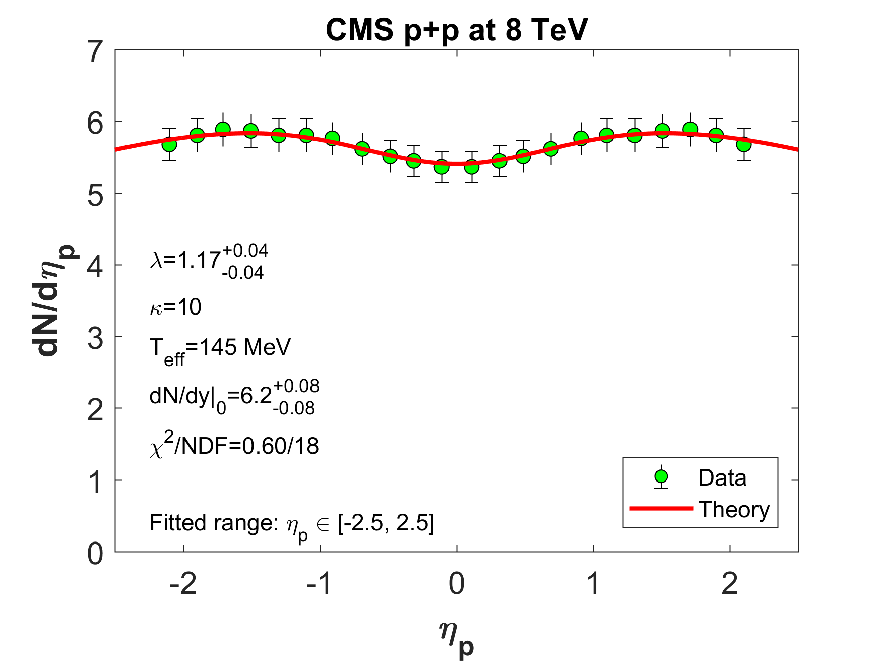
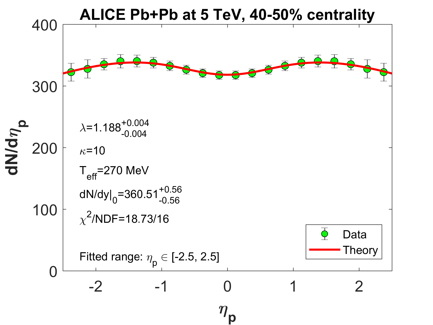
Figure 2: (Left) Fits with the CKCJ hydro solution [6], to CMS p+p data at $\sqrt{s}=$ 8 TeV [13] using a fixed $T_{\rm eff}=145$ MeV. (Right) Similar fits, but for ALICE Pb+Pb data at $\sqrt{s_{NN}}$$=$$5.02$ TeV  [14] in the 40-50 % centrality class, using a fixed $T_{\rm eff}=270$ MeV. The speed of sound is $c_{s}^{2}=1/\kappa=0.1$, fixed in both cases.

The CKCJ hydro solution [6] apparently describes the pseudo-rapidity distributions measured by the CMS experiment in p+p collisions at $\sqrt{s}=$ 8 TeV  [13] in a reasonable manner, for a fixed $T_{\rm eff}=145$ MeV, as indicated by its fit result on the left panel of Fig.  2, Similarly, the CKCJ hydro solution fits the recent ALICE Pb+Pb data at $\sqrt{s_{NN}}$$=$$5.02$ TeV  [14], in the 40-50 % centrality class, using a fixed $T_{\rm eff}=270$ MeV. The speed of sound is fixed in both cases to a realistic value of $c_{s}^{2}=1/\kappa=0.1$  [7].

The conditions of validity of these approximations were detailed in ref. [6]. Typically, these conditions can be simplified for realistic cases to the condition that the fits are done near to mid-rapidity, with $|y|<1/(\lambda-1)$. For $\lambda$ values reported in this paper, these conditions are satisfied. Another requirement is that the parametric curves of these solutions correspond to unique functions of $\eta_{x}$. Typical limits from this condition range from $|\eta_{x}|<1.0$ to $2.5$. For this reason, and in order to reduce the effects of fit range dependencies, in this work we compare fits to various proton-proton and heavy ion collision data by limiting the fit range uniformly to $|\eta_{x}|<2.5$.

5 Discussion

It is interesting to compare the CKCJ solution discussed in the body of this manuscript to other, well known exact solution of 1+ 1 dimensional solutions of perfect fluid hydrodynamics.

It is rather straight-forward to show, that this class of solutions includes the Hwa-Bjorken boost-invariant solutions of ref. [8, 9], as detailed in ref. [6]. This can be obtained as taking the $H\ll 1$ limiting case first, and subsequently evaluating the $\lambda\rightarrow 1$ from above limit. In this case, we obtain that the fluid rapidity $\Omega$ becomes identical with the space-time rapidity $\eta_{x}$, the solution becomes boost-invariant and the rapidity distribution becomes flat.

It is interesting to note a similarity with Landau’s regular solution,  [2, 4] valid also near mid-rapidity, outside the shock-wave region: In these solutions, the fluid rapidity $\Omega$ and the temperature $T$ are used to express the coordinates $(t,r_{z})=(\,t(T,\Omega),\,r_{z}(T,\Omega))$, while in our CKCJ solutions, the dependence on the longitudinal proper time $\tau$ is explicitely given, however the dependence on the space-time rapidity $\eta_{x}$ is given - similarly to Landau’s case- as a parametric curve in terms of the fluid rapidity $\Omega$.

The Csörgő-Grassi-Hama-Kodama (CGHK) family of solutions of ref. [18] is also recovered easily, in the limit of vanishing acceleration, that corresponds to $\lambda\rightarrow 1$ from above.

The Csörgő-Nagy-Csanád or CNC family of solutions of refs. [10, 11] can be recovered, too, but only carefully, given that in the $\kappa\rightarrow 1$, and the $\lambda\rightarrow 1$ limits are not interchangeable. First of all, one has to start from a rewrite of the solutions to the $1\leq\kappa<\lambda$ domain of the parameters, which is not discussed here due to space limitations, one has to take the $\kappa\rightarrow 1$ limit only after this rewrite to recover the CNC solutions.

It is also very interesting to compare our results with the Bialas-Janik-Peschanski or BJP solution of ref. [19]. A main feature of the BJP solutions is that the fluid rapidity distribution evolves in time in an equation of state dependent manner, and approaches asymptotically the Bjorken limit at every fixed value of the coordinate $r_{z}$ for sufficiently late times. In this sense the BJP solutions initially are similar to a static Landau solution (but without the finite lengthscale, the ”l” parameter of Landau’s solution), while at the end of the time evolution they asymptotically converge to a Hwa-Bjorken flow velocity field. Our solutions reviewed here are different in the sense that as a function of the space-time rapidity $\eta_{x}$ the fluid rapidity $\Omega$ is independent of the proper-time $\tau$ so the time evolution of the flow field is only apparent, in our case it is due only to the change of variables from proper-time to time. A similarity to the BJP solution and to Landau’s solution is that our solution is obtained for an arbitrary but constant value of the speed of sound.

For more detailed discussions and comparisons of other solutions with data, we refer to Section 2 of ref. [6].

6 Summary

This is the first part of a series of two papers, where we have highlighted some of the properties of a very recently found, new family of analytic and accelerating, exact and finite solutions of relativistic perfect fluid hydrodynamics for 1+1 dimensionally expanding fireball, evaluated the rapidity and the pseudorapidity densities from these solutions and demonstrated, that these results describe well the pseudorapidity densities of proton-proton collisions at 8 TeV colliding energy as measured by the CMS Collaboration at LHC. Similarly, this solution also describes the pseudorapidity densities in Pb+Pb collisions at $\sqrt{s_{NN}}$$=$$5.02$ TeV measured by the ALICE Collaboration at CERN LHC. These results indicate that the longitudinal expansion dynamics in proton-proton collisions at CERN LHC is very similar to heavy ion collisions at the nearly the same center of mass energies.

Our results confirm similar findings, published recently in ref. [17], that was based on the analytically more restricted and simpler, 1+1 dimensional Csörgő-Nagy-Csanád solutions of refs. [10, 11] . These results also suggest that the space-time rapidity and the fluid rapidity apparently remain nearly proportional to each other, even if the speed of sound implemented in two different solutions becomes very different from one another.

References

- [1] E. Fermi, Prog. Theor. Phys. 5, 570 (1950).
- [2] L. D. Landau, Izv. Akad. Nauk Ser. Fiz. 17, 51 (1953).
- [3] Khalatnikov, I. M. Zur. Eksp. Teor. Fiz. 27 (1954) 529.
- [4] S. Z. Belenkij and L. D. Landau, Nuovo Cim. Suppl. 3S10, 15 (1956) [Usp. Fiz. Nauk 56, 309 (1955)].
- [5] R. Derradi de Souza, T. Koide and T. Kodama, Prog. Part. Nucl. Phys. 86, 35 (2016) [arXiv:1506.03863 [nucl-th]].
- [6] T. Csörgő, G. Kasza, M. Csanád and Z.F. Jiang, Universe 2018, 4(6), 69; [arXiv:1805.01427 [nucl-th]].
- [7] A. Adare et al. [PHENIX Collaboration], Phys. Rev. Lett. 98, 162301 (2007) [nucl-ex/0608033].
- [8] R. C. Hwa, Phys. Rev. D 10, 2260 (1974).
- [9] J. D. Bjorken, Phys. Rev. D 27, 140 (1983).
- [10] T. Csörgő, M. I. Nagy and M. Csanád, Phys. Lett. B 663, 306 (2008) [nucl-th/0605070].
- [11] M. I. Nagy, T. Csörgő and M. Csanád, Phys. Rev. C 77, 024908 (2008) [arXiv:0709.3677 [nucl-th]].
- [12] T. Csörgő, M. I. Nagy and M. Csanád, J. Phys. G 35, 104128 (2008) [arXiv:0805.1562 [nucl-th]].
- [13] S. Chatrchyan et al. [CMS and TOTEM Collaborations], Eur. Phys. J. C 74, no. 10, 3053 (2014) doi:10.1140/epjc/s10052-014-3053-6 [arXiv:1405.0722 [hep-ex]].
- [14] J. Adam et al. [ALICE Collaboration], Phys. Rev. Lett. 116, no. 22, 222302 (2016) doi:10.1103/PhysRevLett.116.222302 [arXiv:1512.06104 [nucl-ex]].
- [15] T. Csörgő and B. Lörstad, Phys. Rev. C 54, 1390 (1996) doi:10.1103/PhysRevC.54.1390 [hep-ph/9509213].
- [16] M. Csanád, T. Csörgő, Z. F. Jiang and C. B. Yang, Universe 3, no. 1, 9 (2017) [arXiv:1609.07176 [hep-ph]].
- [17] Z.-F. Jiang, C.-B. Yang, M. Csanád and T. Csörgő, Phys. Rev. C 97, no. 6, 064906 (2018) [arXiv:1711.10740 [nucl-th]].
- [18] T. Csörgő, F. Grassi, Y. Hama and T. Kodama, Phys. Lett. B 565, 107 (2003) [nucl-th/0305059].
- [19] A. Bialas, R. A. Janik and R. B. Peschanski, Phys. Rev. C 76, 054901 (2007) doi:10.1103/PhysRevC.76.054901 [arXiv:0706.2108 [nucl-th]].