Multiscale Fisher’s Independence Test for Multivariate Dependence

Abstract

Identifying dependency in multivariate data is a common inference task that arises in numerous applications. However, existing nonparametric independence tests typically require computation that scales at least quadratically with the sample size, making it difficult to apply them in the presence of massive sample sizes. Moreover, resampling (e.g., permutation) is usually necessary to evaluate the statistical significance of the resulting test statistics at finite sample sizes, further worsening the computational burden. We introduce a scalable, resampling-free approach to testing the independence between two random vectors by breaking down the task into simple univariate tests of independence on a collection of $2\times 2$ contingency tables constructed through sequential coarse-to-fine discretization of the sample space, transforming the inference task into a multiple testing problem that can be completed with almost linear complexity with respect to the sample size. To address increasing dimensionality, we introduce a coarse-to-fine sequential adaptive procedure that exploits the spatial features of dependency structures. We derive a finite-sample theory that guarantees the inferential validity of our adaptive procedure at any given sample size. We show that our approach can achieve strong control of the level of the testing procedure at any sample size without resampling or asymptotic approximation and establish its large-sample consistency. We demonstrate through an extensive simulation study its substantial computational advantage in comparison to existing approaches while achieving robust statistical power under various dependency scenarios, and illustrate how the divide-and-conquer nature can be exploited to not just test independence but to learn the nature of the underlying dependency. Finally, we demonstrate the use of our method through analyzing a dataset from a flow cytometry experiment.

Keywords: Nonparametric inference, multiple testing, unsupervised learning, scalable inference, massive data

1 Introduction

Testing independence and learning the dependency structure in multivariate problems has been a central inference task since the very beginning of modern statistics, and the last two decades have witnessed a surge of interest in this problem among statisticians, engineers, and computer scientists. A variety of different methods have been proposed for testing independence between two random vectors. For example, Székely and Rizzo, (2009) generalize the product-moment covariance and correlation to the distance covariance and correlation. Bakirov et al., (2006), Fan et al., (2017), and Meintanis and Iliopoulos, (2008) all developed nonparametric tests of independence based on the distance between the empirical joint characteristic function of the random vectors and the product of the marginal empirical characteristic functions of the two random vectors. Székely and Rizzo, (2013) further consider an asymptotic scenario with the dimensionality of the vectors increasing to infinity while keeping the sample size fixed. In a different vein, Heller et al., (2013) form a test based on univariate tests of independence between the distances of each of the random vectors from a central point. In machine learning, a class of kernel-based tests has also become popular. For example, Gretton et al., (2008) form a test based on the eigenspectrum of covariance operators in a reproducing kernel Hilbert spaces (RKHS). More recently, Pfister et al., (2018) generalized this approach to the multivariate case by embedding the joint distribution into an RKHS. Weihs et al., (2018) defined a class of multivariate nonparametric measures which leads to multivariate extensions of the Bergsma-Dassios sign covariance. Lee et al., (2019) proposed using random projections to reduce multivariate independence testing to a univariate problem, and complete the latter using an ensemble approach combining the distance correlation and a binary expansion test statistic (Zhang,, 2019).

The existing multivariate independence tests generally require the computation of statistics at a computational complexity that scales at least quadratically in the sample size, making them impractical for data sets with sample sizes greater than, say, tens of thousands of observations. Many of these multivariate methods also require resampling – in the form of either permutation or bootstrap – to evaluate statistical significance. This additional computational burden makes applications of these methods computationally expensive even for problems with moderate sample sizes. To overcome these challenges, some appeal to asymptotic approximations (either in large $n$ or in large $p$) (Székely and Rizzo,, 2013; Pfister et al.,, 2018) to derive procedures that when the asymptotic conditions are satisfied do not require resampling. However, because it is hard to judge whether such conditions are true in multivariate settings, practitioners usually still resort to resampling to ensure validity.

A scalable testing strategy for data with massive sample sizes should ideally achieve (i) close to linear computational complexity in the sample size and (ii) finite-sample guarantees without the need for resampling or asymptotic approximation. We aim to introduce a framework that achieves these two desiderata. Specifically, instead of calculating a single test statistic for independence all at once, we take a multi-scale divide-and-conquer approach that breaks apart the nonparametric multivariate test of independence into simple univariate independence tests on a collection of $2\times 2$ contingency tables defined by sequentially discretizing the original sample space at a cascade of scales. This approach transforms a complex nonparametric testing problem into a multiple testing problem involving simple tests that can be carried out efficiently. While such an approach was previously adopted in Ma and Mao, (2019) for testing the independence between two scalar variables, the increasing dimensionality in the multivariate setting makes a brute-force, exhaustive approach as proposed therein computationally prohibitive and statistically inefficient. As such we incorporate data-adaptivity into the framework and introduce a coarse-to-fine sequential adaptive testing procedure which exploits the spatial characteristics of dependency structures to drastically reduce the number of univariate tests completed in the procedure. At the same time, we derive a finite-sample theory showing that even with the additional adaptivity, exact inference (in terms of controlling the level of the test) can be achieved at any given sample size without resorting to either resampling or large-sample approximation.

Aside from these properties, our approach also enjoys a unique feature of practical relevance—its divide-and-conquer nature allows learning the structure of the underlying dependency. By identifying and visualizing the $2\times 2$ tables on which the univariate independence test returns the most significant $p$-values, we can identify using MultiFIT interesting dependency relationships otherwise hidden by the multivariate nature of the sample space and the complexity of the joint distribution.

We carry out extensive simulation studies that examine the computational scalability and statistical power of our method in a variety of dependency scenarios and compare our method to a number of state-of-the-art approaches. We demonstrate an application of our method to a data set from a flow cytometry experiment with a massive sample size. All technical proofs are provided in the Online Supplementary Materials S1.

2 Method

Our strategy is to transform nonparametric testing of multivariate independence into a multiple testing problem involving univariate independence tests on a collection of $2\times 2$ tables constructed by sequentially partitioning the sample space. In Section 2.1, we start by describing the construction of these $2\times 2$ tables and justify the testing strategy by showing that two random vectors are independent if and only if univariate independence holds on all of the $2\times 2$ tables so constructed. In Section 2.2, we present a data-adaptive sequential testing procedure that completes the univariate tests on only a subset of the $2\times 2$ tables to accommodate increasing dimensionality of the random vectors. Finally in Section 2.3 we derive a finite-sample theory that provides guarantees for the validity of our procedure at any sample size without appealing to resampling or asymptotic approximations, and establish the large-sample consistency for our procedure.

2.1 Multi-scale $2\times 2$ testing for multivariate independence

We start by introducing some notations that will be used throughout the paper as well as some concepts related to nested dyadic partitioning (NDP), which will be used for constructing the $2\times 2$ tables on which univariate independence tests are completed.

Let $\Omega=\Omega_{\mathbf{X}}\times\Omega_{\mathbf{Y}}$ denote a $D$-dimensional joint sample space of two random vectors $\mathbf{X}$ and $\mathbf{Y}$ where $\Omega_{\mathbf{X}}$ and $\Omega_{\mathbf{Y}}$ are respectively the marginal sample space of $\mathbf{X}$ and $\mathbf{Y}$. For simplicity, we assume that $\Omega_{\mathbf{X}}=[0,1]^{D_{x}}$ and $\Omega_{\mathbf{Y}}=[0,1]^{D_{y}}$ – that is, each marginal random variable of the two random vectors is supported on $[0,1]$. This costs no generality as other random variables can be mapped onto the unit interval through a CDF transform.

A partition $\mathcal{P}$ on a set $S$ is a collection of disjoint non-empty subsets of $S$ whose union is $S$. A nested dyadic partition (NDP) on $S$ is a sequence of partitions, $\mathcal{P}^{0},\mathcal{P}^{1},\ldots,\mathcal{P}^{k},\ldots$ such that $\mathcal{P}^{0}=\{S\}$, and for each $k\geq 1$, the sets in $\mathcal{P}^{k}$ are those generated by dividing each set in $\mathcal{P}^{k-1}$ into two children. For example, if we consider an NDP on $[0,1]$ generated from sequantially dividing sets into two halves in the middle of the interval, then we have an NDP such that for $k\geq 0$, $\mathcal{P}^{k}=\left\{\left[\frac{l-1}{2^{k}},\frac{l}{2^{k}}\right)\right\}_{l\in\{1,...,2^{k}\}}$. We refer to this particular NDP as the canonical NDP, and note that $\bigcup\mathcal{P}^{k}$ generates the Borel $\sigma$-algebra. In the following, we shall consider only NDPs that generate the Borel $\sigma$-algebra. Now let us assume that each dimension of $\Omega$ has a corresponding NDP. For our purpose, the NDP for each dimension can be distinct, but for ease of illustration let us assume that they are all the canonical NDPs on $[0,1]$. We consider the cross-products of these marginal NDPs on each dimension, which creates a cascade of partitions on the joint sample space. Specifically, for any vector of non-negative integers $\mathbf{k}=(k_{1},...,k_{D})\in\mathbb{N}_{0}^{D}$, $\mathcal{P}^{k_{1}}\times\cdots\times\mathcal{P}^{k_{D}}$ forms a partition of $\Omega$. The elements of this partition are rectangles of the form

$$A=A_{1}\times A_{2}\times\cdots\times A_{D},\quad\text{with $A_{d}\in\mathcal{P}^{k_{d}}$ for all $d=1,2,\ldots,D$.}$$

Note that the vector $\mathbf{k}$ encodes the level of $A$ in the NDP for each dimension of $\Omega$. That is, $k_{d}$ is the level of the NDP on $[0,1]$ to which the $d$th margin of $A$ belongs. From now on, we shall refer to a set $A$ of the above form as a cuboid. We refer to the sum of all $k_{d}$, $r=\sum_{d=1}^{D}k_{d}$, as the resolution of $A$. Figure 1 illustrates a cuboid $A$ of resolution 3 in a 3-dimensional sample space with canonical NDPs on the margins.

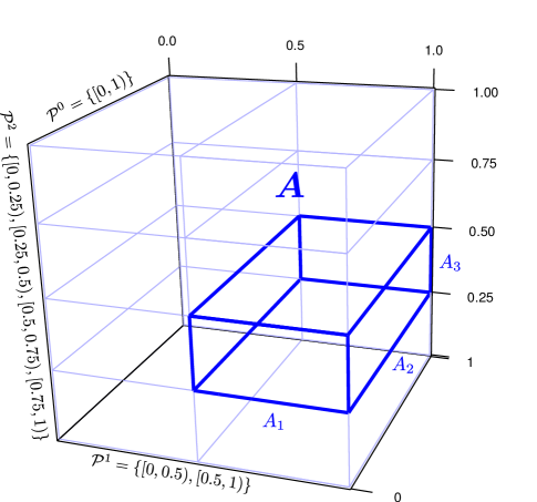
Figure 1: A cuboid of resolution 3 in a 3-dimensional sample space under the canonical NDP.

We are now ready to construct the $2\times 2$ tables on which to carry out univariate tests of independence. One can divide a cuboid $A$ into four blocks according to the NDP along any pair of its margins while keeping all other dimensions intact. For the division involving dimension $i$ of $\mathbf{X}$ and dimension $j$ of $\mathbf{Y}$, we use $A_{ij}^{00}$, $A_{ij}^{01}$, $A_{ij}^{10}$, and $A_{ij}^{11}$ to denote these four blocks. Figure 2 illustrates a division on the cuboid demonstrated in Figure 1.

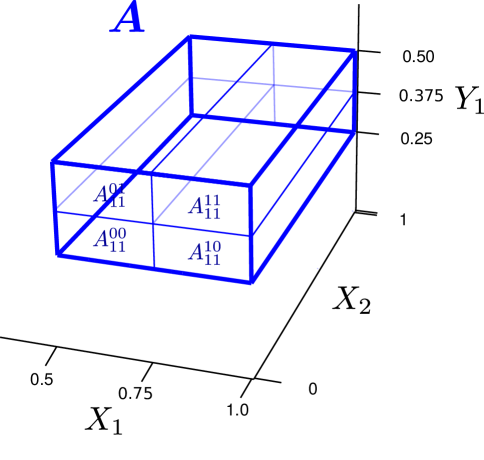
Figure 2: The division of the cuboid $A$ in Figure 1 into four blocks along dimension 1 for $\mathbf{X}$ and dimension 1 for $\mathbf{Y}$.

Suppose now that $F$ is the joint sampling distribution of $(\mathbf{X},\mathbf{Y})$, then for the $2\times 2$ division of $A$ along the $i$th dimension of $\mathbf{X}$ and $j$th dimension of $\mathbf{Y}$, we can define a corresponding odds-ratio that characterizes the dependency in $F$ on the $2\times 2$ division,

$$\theta_{ij}(A)=\frac{F(A_{ij}^{10})F(A_{ij}^{01})}{F(A_{ij}^{00})F(A_{ij}^{11})}.$$

An i.i.d. sample from $F$ will give rise to a $2\times 2$ contingency table formed by the number of data points lying in the four blocks

$$\{n(A_{ij}^{00}),n(A_{ij}^{01}),n(A_{ij}^{10}),n(A_{ij}^{11})\}\quad\text{or}\quad\begin{tabular}[]{|c|c|}\hline\cr$n(A_{ij}^{00})$&$n(A_{ij}^{01})$\\ \hline\cr$n(A_{ij}^{10})$&$n(A_{ij}^{11})$\\ \hline\cr\end{tabular}$$

where $n(A)$ represents the number of data points in $A$.

One can test whether $\theta_{ij}(A)=1$ based on this contingency table. While several standard tests are available for testing independence on a $2\times 2$ table, we adopt Fisher’s exact test. As we will show in Section 2.3, it turns out that the conditional nature of Fisher’s test plays a crucial role in our finite-sample theory—it ensures that the resulting testing procedure obtains exact validity at any finite sample size without resampling or asymptotics. Figure 3 illustrates two contingency tables on which Fisher’s test is applied for a cuboid $A$. In the following, we will use $p_{ij}(A)$ to represent the resulting $p$-value from the test on this particular $2\times 2$ table.

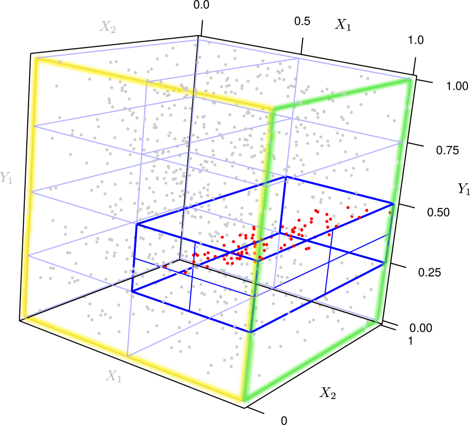
(a)

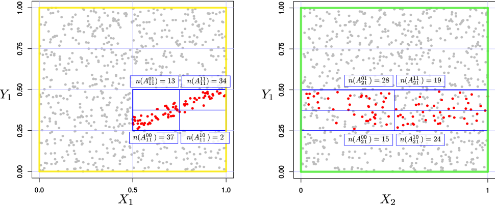
(b)

Figure 3: Illustration of the two $2\times 2$ contingency tables on a cuboid $A$ arising from an i.i.d. sample in which dependency exists in $(X_{1},Y_{1})$

.

How does testing those “local” nulls $\theta_{ij}(A)=1$ relate to our original “global” hypothesis of $\mathbf{X}\mathchoice{\mathrel{\hbox to0.0pt{$\displaystyle\perp$\hss}\mkern 2.0mu{\displaystyle\perp}}}{\mathrel{\hbox to0.0pt{$\textstyle\perp$\hss}\mkern 2.0mu{\textstyle\perp}}}{\mathrel{\hbox to0.0pt{$\scriptstyle\perp$\hss}\mkern 2.0mu{\scriptstyle\perp}}}{\mathrel{\hbox to0.0pt{$\scriptscriptstyle\perp$\hss}\mkern 2.0mu{\scriptscriptstyle\perp}}}\mathbf{Y}$? It is obvious that if $\mathbf{X}\mathchoice{\mathrel{\hbox to0.0pt{$\displaystyle\perp$\hss}\mkern 2.0mu{\displaystyle\perp}}}{\mathrel{\hbox to0.0pt{$\textstyle\perp$\hss}\mkern 2.0mu{\textstyle\perp}}}{\mathrel{\hbox to0.0pt{$\scriptstyle\perp$\hss}\mkern 2.0mu{\scriptstyle\perp}}}{\mathrel{\hbox to0.0pt{$\scriptscriptstyle\perp$\hss}\mkern 2.0mu{\scriptscriptstyle\perp}}}\mathbf{Y}$ then independence must hold—that is, $\theta_{ij}(A)=1$—for any $A$ and any pair of $X$-$Y$ margins $i$ and $j$. However, the reverse is not obvious—does independence on these $2\times 2$ tables formed under the marginal NDPs also imply that $\mathbf{X}$ and $\mathbf{Y}$ are independent? If this is the case, then one can test for independence between $\mathbf{X}$ and $\mathbf{Y}$ by testing whether $\theta_{ij}(A)=1$ on the $2\times 2$ tables. The next theorem confirms that this is indeed the case.

Theorem 2.1.

$\mathbf{X}\mathchoice{\mathrel{\hbox to0.0pt{$\displaystyle\perp$\hss}\mkern 2.0mu{\displaystyle\perp}}}{\mathrel{\hbox to0.0pt{$\textstyle\perp$\hss}\mkern 2.0mu{\textstyle\perp}}}{\mathrel{\hbox to0.0pt{$\scriptstyle\perp$\hss}\mkern 2.0mu{\scriptstyle\perp}}}{\mathrel{\hbox to0.0pt{$\scriptscriptstyle\perp$\hss}\mkern 2.0mu{\scriptscriptstyle\perp}}}\mathbf{Y}$ if and only if $\theta_{ij}(A)=1$ for all pairs of dimension $i$ of $\mathbf{X}$ and dimension $j$ of $\mathbf{Y}$ on all cuboids $A$.

This theorem implies that one can in principle test for independence between two random vectors $\mathbf{X}$ and $\mathbf{Y}$ by exhaustively testing whether independence holds on each of the $2\times 2$ tables constructed on all cuboids up to some maximum resolution, aimed at identifying dependency structures up to a certain level of detail. This boils down to a multiple testing problem involving a collection of $p$-values computed on all of the $2\times 2$ tables up to the maximal resolution. However, such a brute-force exhaustive scan is not practical when the dimensionality grows. If one were to exhaustively test independence on all possible $2\times 2$ tables of all cuboids up to even just a moderate resolution, the number of tests required would quickly become prohibitive. Specifically, the total number of tests to be completed up to a resolution of $R$ is $\sum_{\rho=0}^{R}D_{x}\cdot D_{y}\cdot 2^{\rho}\cdot{{\rho+D-1}\choose{D-1}}$.

For multivariate problems of more than a handful of dimensions then, one must be selective in carrying out the univariate tests. Beyond the consideration of computational practicality, reducing the number of tests is also desirable for the sake of statistical performance. Every additional test comes with a price in multiple testing control, and thus it is important to be discreet in choosing the tests to complete.

2.2 MultiFIT: a coarse-to-fine adaptive testing procedure

Given the above considerations, we propose a data-adaptive strategy that selects in each resolution a subset of the available tables to test based on the statistical evidence attained on coarser resolutions. In particular, only the “children” of tables in the previous resolution whose $p$-values are below a pre-specified threshold are selected for testing. Figure 4 provides an illustration. Suppose that cuboid $A$ in resolution $r$ satisfies $p_{ij}(A)<p^{*}$, some preset threshold, then the four children cuboids, generated by dividing $A$ in the $i$th or the $j$th dimensions are tested in resolution $r+1$. This coarse-to-fine testing procedure terminates at a maximal resolution $R_{max}$ or when no cuboids at the current resolution have $p$-values passing the threshold.

Figure 4: The selection of tables for testing based on the statistical evidence on their parent. The two right children correspond to dividing $A$ along the margin that corresponds to the $i$th margin of $\mathbf{X}$, and the two left children correspond to dividing $A$ along the margin that corresponds to the $j$th margin of $\mathbf{Y}$. Those four children are tested in resolution $r+1$ if their parent $A$ in resolution $A$ produces a $p$-value below the threshold $p^{*}$.

The rationale behind this strategy is to exploit the spatial smoothness of dependency structures—when $\mathbf{X}$ and $\mathbf{Y}$ are dependent, adjacent and nested cuboids tend to contain empirical evidence for the dependency in a “correlated” manner. (It is worth noting that here the “correlation” corresponds to our assumption about the underlying sampling distribution that its dependency structure is spatially smooth, not the sampling behavior of the data points given the sampling distribution.) Thus using the statistical evidence at coarser resolutions to inform which cuboids to test in finer resolutions can lead to effective detection of the dependency structure.

Next we formally present the adaptive testing procedure. We let $\mathcal{C}^{(r)}$ denote the collection of cuboids at resolution $r$ on which we carry out independence tests over all of the corresponding $D_{x}\cdot D_{y}$ $2\times 2$ tables, one for each $(i,j)$ pair of margins, where $i$ and $j$ are the indices for the $X$ and $Y$ margins respectively. The procedure consists of three components:

1. Initialization: Let $\mathcal{C}^{(0)}$ be $\Omega$, and let $\mathcal{C}^{(r)}=\emptyset$ for $1\leq r\leq R_{max}$.

2. Coarse-to-fine scanning: For $r=0,1,2,\ldots,R_{max}$ do the following:

   • Independence testing: Apply Fisher’s exact test of independence to the $D_{x}\cdot D_{y}$ $2\times 2$ tables of each cuboid $A\in\mathcal{C}^{(r)}$ and record the $p$-values.

   • Selection of cuboids to test for the next resolution: When $r<R_{max}$, if the $(i,j)$-table for a cuboid $A\in\mathcal{C}^{(r)}$ has a $p$-value more significant than a threshold $p^{*}$, add to $\mathcal{C}^{(r+1)}$ the four child cuboids of $A$ generated from dividing $A$ along the $i$th and the $j$th dimensions respectively, each generating two children.

3. Multiple testing control: Apply any valid multiple testing control procedure on the entire set of $p$-values generated by the algorithm, thereby controlling the level of the entire testing procedure at $\alpha$.

Although the data-adaptive selection in Step 1b is designed to overcome the explosive number of tests required when the dimensionality is large, it is still often feasible to apply exhaustive testing up to some resolution $R^{*}<R_{max}$. In other words, one can test on all available cuboids up to resolution $R^{*}$, and let the adaptive selection of the cuboids in Step 1b kick in for resolutions beyond $R^{*}$. In our software, we allow the user to specify a resolution $R^{*}$ below which exhaustive testing is adopted. A smaller value for $R^{*}$ will favor the detection of more global signals, while a larger $R^{*}$ will favor localized signals.

In our implementation of the testing procedure, we consider two different approaches for achieving the multiple testing control in Step 2.

Strategy I. A holistic approach to multiple testing. Under this strategy, one applies multiple testing control procedure on the entire set of $p$-values generated in Step 1 of MultiFIT all at once, regardless of the resolution of the corresponding table. Simple choices of the multiple testing devices include Bonferroni are Holm corrections.

Strategy II. A resolution-specific approach to multiple testing. Under this strategy, one applies multiple testing control in two stages—first on the $p$-values within each resolution level, producing an intermediate, intra-resolution significance level for each resolution, and then in the second stage further correct these intra-resolution “$p$-values” over all the resolutions, which will produce a valid, corrected overall $p$-value for testing the global null hypothesis of independence. This strategy has the benefit that one can now “allocate” a fixed level budget to each resolution, and thus avoids the possibility of loss in power due to having many more tables tested in high resolutions than coarse ones. This method is generally more powerful than the holistic approach above for testing the global null hypothesis when a dependency structure exists in coarser resolutions.

An additional benefit of the resolution-specific approach is that it can be implemented with early stopping so that the MultiFIT procedure can terminate as soon as there is sufficient evidence for rejecting the global null in the first few resolutions without continuing into testing on higher resolutions. This is possible because in this approach we bound the influence of tables in finer resolutions on the (corrected) significance level of tests in coarser resolutions. Our software implements this early stopping strategy for the resolution-specific approach to multiple testing when Holm’s method is used for intra-resolution correction along with Bonferroni’s method for cross-resolution correction. Early stopping can reduce the time complexity significantly in the presence of a global signal (see Figure 6).

Detailed pseudo-code for the procedure is provided in Supplement S2. We call this testing procedure MultiFIT, which stands for Multi-scale Fisher’s Independence Test.

2.3 Finite-sample validity and large-sample consistency

Because MultiFIT formulates the test of independence as a multiple testing problem, its inferential validity rests on whether the $p$-values are indeed valid, i.e., that they are stochastically larger than a uniform random variable under the null hypothesis. Note that the $p$-values for the cuboids selected in the MultiFIT procedure are computed according to the (central) hypergeometric null distribution on the $2\times 2$ tables. At first glance, these null distributions appear to ignore the data-adaptive selection of a cuboid $A$ based on the evidence in its ancestral cuboids. As such, one may suspect that there might be a selection bias that causes such $p$-values to lose their face values.

The following theorem and corollary resolve this concern by showing that, interestingly, the distribution of all the selected $2\times 2$ tables given their marginal totals are independent of the event that they are selected in the procedure, and hence the $p$-values computed in the procedure are indeed still valid despite the adaptive sequential selection. Consequently, one can indeed control the level of the entire procedure using multiple testing methods based on these $p$-values.

Theorem 2.2.

Under the null hypothesis $\mathbf{X}\mathchoice{\mathrel{\hbox to0.0pt{$\displaystyle\perp$\hss}\mkern 2.0mu{\displaystyle\perp}}}{\mathrel{\hbox to0.0pt{$\textstyle\perp$\hss}\mkern 2.0mu{\textstyle\perp}}}{\mathrel{\hbox to0.0pt{$\scriptstyle\perp$\hss}\mkern 2.0mu{\scriptstyle\perp}}}{\mathrel{\hbox to0.0pt{$\scriptscriptstyle\perp$\hss}\mkern 2.0mu{\scriptscriptstyle\perp}}}\mathbf{Y}$,

$$n(A^{00}_{ij})\mathchoice{\mathrel{\hbox to0.0pt{$\displaystyle\perp$\hss}\mkern 2.0mu{\displaystyle\perp}}}{\mathrel{\hbox to0.0pt{$\textstyle\perp$\hss}\mkern 2.0mu{\textstyle\perp}}}{\mathrel{\hbox to0.0pt{$\scriptstyle\perp$\hss}\mkern 2.0mu{\scriptstyle\perp}}}{\mathrel{\hbox to0.0pt{$\scriptscriptstyle\perp$\hss}\mkern 2.0mu{\scriptscriptstyle\perp}}}\mathbf{1}(A\in\mathcal{C}^{(r)})\,|\,n(A^{0\cdot}_{ij}),n(A^{\cdot 0}_{ij}),n(A)$$

for all cuboids $A$ of resolution $r$ and all pairs $(i,j)$ of the margins, where $n(A^{0\cdot}_{ij})=n(A^{00}_{ij})+n(A^{01}_{ij})$ and $n(A^{\cdot 0}_{ij})=n(A^{00}_{ij})+n(A^{10}_{ij})$, and $\mathbf{1}(A\in\mathcal{C}^{(r)})$ is the indicator for the event that $A$ is selected to be tested in the MultiFIT procedure.

In other words, for any cuboid $A$, the conditional distribution of the $2\times 2$ table on each pair of $X$-$Y$ margins given the corresponding marginal totals is the same central hypergeometric distribution when $\mathbf{X}\mathchoice{\mathrel{\hbox to0.0pt{$\displaystyle\perp$\hss}\mkern 2.0mu{\displaystyle\perp}}}{\mathrel{\hbox to0.0pt{$\textstyle\perp$\hss}\mkern 2.0mu{\textstyle\perp}}}{\mathrel{\hbox to0.0pt{$\scriptstyle\perp$\hss}\mkern 2.0mu{\scriptstyle\perp}}}{\mathrel{\hbox to0.0pt{$\scriptscriptstyle\perp$\hss}\mkern 2.0mu{\scriptscriptstyle\perp}}}\mathbf{Y}$ whether or not we condition on the event that cuboid $A$ is selected to be tested in the MultiFIT procedure. As such, the $p$-values from the Fisher’s exact tests applied on the adaptively selected tables in our procedure can be treated at face value, which justifies using multiple testing adjustment based on these $p$-values to control the level.

Corollary 2.1.

The $p$-values computed during Step 1 of the MultiFIT procedure are valid, and thus Step 2 of the procedure can control the level of the entire testing procedure at any given level $\alpha$.

The above theorem and corollary provide a strong theoretical guarantee—unavailable to other existing methods—that MultiFIT attains exact control of the level at any finite sample size. This is an extremely important property in that for multivariate sample spaces traditional large $n$ asymptotic controls of the level can often be inaccurate, and existing methods typically appeal to resampling strategies such as permutation to provide approximate finite-sample control of the level. But permutation is often computationally prohibitive in this context in that even just a single run of a test can be expensive, not to mention applying the same test hundreds to thousands of times. In contrast, MultiFIT achieves exact control of the level by a single run of the procedure without resampling. We offer a numerical validation of level control through simulations in Section S4.

We also note that the proof of Theorem 2.2 turns out to be conceptually interesting and elucidates why the adoption of the Fisher’s exact test on each $2\times 2$ table is critical to ensuring the exact finite sample validity of the MultiFIT procedure. In particular, the event that a cuboid $A$ is selected to be tested in MultiFIT is in the $\sigma$-algebra generated by the $p$-values on all of its ancestral cuboids, which can be shown to be independent of the counts in the $2\times 2$ table on $A$ under the null hypothesis of independence once the corresponding marginal totals are conditioned upon. This independence is elucidated under a Bayesian network representation of the multivariate central hypergeometric (CHG) distribution (Ma and Mao,, 2019, Theorem 3). Accordingly, conditioning on the selection of a cuboid under MultiFIT does not alter the null distribution of the $p$-values for the $2\times 2$ tables on that cuboid, and thus the validity of the procedure is maintained even with the adaptive selection of the tables to test on. Below we provide a sketch of the proof for Theorem 2.2 for interested readers and defer the technical details to Supplement S1.

Sketch of Proof for Theorem 2.2: For two non-negative integers $a$ and $b$, let $\mathbf{n}_{a,b}$ denote a $2^{a}\times 2^{b}$ contingency table formed by a cross-product of a marginal partition on $\mathbf{X}$ at depth $a$ and a marginal partition on $\mathbf{Y}$ at depth $b$. Specifically, it is the $2^{a}\times 2^{b}$ contingencey table corresponding to a partition $\mathcal{P}^{k_{1}}\times\cdots\times\mathcal{P}^{k_{D}}$ of $\Omega$, where $\sum_{d=1}^{D_{x}}k_{d}=a$ and $\sum_{d=D_{x}+1}^{D}k_{d}=b$. Under the null hypothesis that $\mathbf{X}\mathchoice{\mathrel{\hbox to0.0pt{$\displaystyle\perp$\hss}\mkern 2.0mu{\displaystyle\perp}}}{\mathrel{\hbox to0.0pt{$\textstyle\perp$\hss}\mkern 2.0mu{\textstyle\perp}}}{\mathrel{\hbox to0.0pt{$\scriptstyle\perp$\hss}\mkern 2.0mu{\scriptstyle\perp}}}{\mathrel{\hbox to0.0pt{$\scriptscriptstyle\perp$\hss}\mkern 2.0mu{\scriptscriptstyle\perp}}}\mathbf{Y}$, the sampling distribution of any such table $\mathbf{n}_{a,b}$ given all of its row totals and column totals is a multivariate CHG distribution.

By Theorem 3 in Ma and Mao, (2019), a draw from the central multivariate hypergeometric distribution such as $\mathbf{n}_{a,b}$ can actually be generated inductively from coarse-to-fine resolutions using univariate CHG distributions. Specifically, suppose we have already generated the table $\mathbf{n}_{a-1,b}$ and $\mathbf{n}_{a,b-1}$, then the conditional distribution of $\mathbf{n}_{a,b}$ given its row and column totals, as well as the two “parent” tables $\mathbf{n}_{a-1,b}$ and $\mathbf{n}_{a,b-1}$, are simply a collection of independent univariate central hypergeometric distributions—one for each adjacent $2\times 2$ subtables in $\mathbf{n}_{a,b}$ given its row totals and column totals, which correspond to cell counts in $\mathbf{n}_{a-1,b}$ and $\mathbf{n}_{a,b-1}$.

Let $A$ be a cuboid that arises from dividing the $\mathbf{X}$ margins a total of $r_{x}$ times and the $\mathbf{Y}$ margins a total of $r_{y}$ times. The above reasoning implies that one can show by construction that for any $2\times 2$ table on a cuboid $A$, there exists a Bayesian network in the form presented in Figure 5 such that the total number of observations in $A$, $n(A)$, is an element in the contingency table $\mathbf{n}_{r_{x},r_{y}}$ (the node with bold black boundary in Figure 5), the counts for the four blocks of the $2\times 2$ table, $n(A_{ij}^{00})$, $n(A_{ij}^{01})$, $n(A_{ij}^{10})$, and $n(A_{ij}^{11})$, are in $\mathbf{n}_{r_{x}+1,r_{y}+1}$ (the node with blue dashed boundary in Figure 5), and the marginal totals of $A$ are in $\mathbf{n}_{r_{x}+1,r_{y}}$ and $\mathbf{n}_{r_{x},r_{y}+1}$ (the two nodes with dotted red boundaries in Figure 5). In addition, the counts of all of the $2\times 2$ tables on ancestors of $A$ are measurable with respect to the $\sigma$-algebra generated the gray-shaded nodes in the Bayesian network, and thus are independent of the $2\times 2$ table on $A$ given the marginal totals. Therefore the selection of a table does not influence the null distribution once the marginal totals are conditioned upon, as such conditioning blocks all the paths from these ancestral nodes to the blue dashed node.

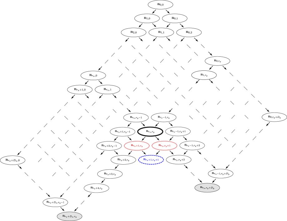
Figure 5: A Bayesian network augmentation for the multivariate CHG model on contingency tables formed by cross-products of sequential marginal partitions on $\Omega_{\mathbf{X}}$ and those on $\Omega_{\mathbf{Y}}$.

Now that we have established the finite-sample exact validity of the MultiFIT procedure, our last theoretical result shows that when the sample size $n$ grows, under certain conditions MultiFIT can consistently reject the null hypothesis of independence.

Theorem 2.3 (Large-sample consistency).

Suppose $\mathbf{X}$ and $\mathbf{Y}$ are not independent under their sampling distribution $F$. Let $(\mathbf{X}_{1},\mathbf{Y}_{1}),(\mathbf{X}_{2},\mathbf{Y}_{2}),\ldots,(\mathbf{X}_{n},\mathbf{Y}_{n})$ be i.i.d. observations from $F$. As $n\rightarrow\infty$, suppose one of the following is true

• $R^{*}$ is fixed but large enough such that there exists at least one cuboid $A$ of resolution $r\leq R^{*}$ with $\theta_{ij}(A)\neq 1$ for some pairs of margin $(i,j)$,

• $R^{*}\rightarrow\infty$ and it is $o(\log n)$.

Then the power for MultiFIT to reject the null hypothesis that $\mathbf{X}\mathchoice{\mathrel{\hbox to0.0pt{$\displaystyle\perp$\hss}\mkern 2.0mu{\displaystyle\perp}}}{\mathrel{\hbox to0.0pt{$\textstyle\perp$\hss}\mkern 2.0mu{\textstyle\perp}}}{\mathrel{\hbox to0.0pt{$\scriptstyle\perp$\hss}\mkern 2.0mu{\scriptstyle\perp}}}{\mathrel{\hbox to0.0pt{$\scriptscriptstyle\perp$\hss}\mkern 2.0mu{\scriptscriptstyle\perp}}}\mathbf{Y}$ converges to 1.

2.4 Practical considerations in applying MultiFIT

We close this section by discussing some practical aspects in applying the MultiFIT procedure. We set the default value for the p-value threshold $p^{*}$ in our software for resolutions higher than $R^{*}$ at $(D_{x}\cdot D_{y}\cdot\log_{2}(n))^{-1}$. This keeps the number of $2\times 2$ tables tested constant (on average) under the null hypothesis irrespective of the number of dimensions, while also making the threshold more stringent with increasing sample size in such a way that makes the total number of tables scales roughly linearly with the sample size, which we will confirm numerically in the next section.

We note that under this strategy of setting $p^{*}$, we get that for certain alternatives, in particular those that are pervasive over the sample space and involve a large number of cuboids, the complexity of the MultiFIT procedure may be higher than $O(n\log n)$. Such large-scale, global alternatives, however, can usually be detected in coarse resolutions, and thus in practice when the algorithm is equipped with early stopping it will in fact run faster with larger $n$ under such alternatives. If the practitioner wishes to ensure a strict $O(n\log n)$ bound on the computational complexity with or without incorporating early stopping, a simple approximate version of the MultiFIT algorithm can achieve this. Specifically, in Step 1b of MultiFIT, instead of including child cuboids of all cuboids $A$ with p-value less than $p^{*}$, we can include only child cuboids with p-value less than $p^{*}$ up to a maximum number of cuboids $A$ (e.g., 100) with the smallest Fisher’s p-values. This alternative constraint ensures that the computational cost of MultiFIT algorithm is strictly bounded at $O(n\log n)$. While under this approximation the conditions for ensuring the finite-sample guarantees are no longer satisfied, we found in practice that its statistical power (Figure 8 and Figure 9) and level (Figure S4) hardly differs from those of the exact MultiFIT procedure in essentially all of the numerical settings we have encountered.

3 Numerical Examples

3.1 Computational Scalability

Because computational scalability is a key motivation for our approach, we start by evaluating the computational scalability of MultiFIT with those of three other state-of-the-art methods with well-documented software—the Heller-Heller-Gorfine (HHG) multivariate test of association from Heller et al., (2013), the Distance Covariance (DCov) method of Székely and Rizzo, (2009), and the kernel-based method (dHSIC) of Pfister et al., (2018).

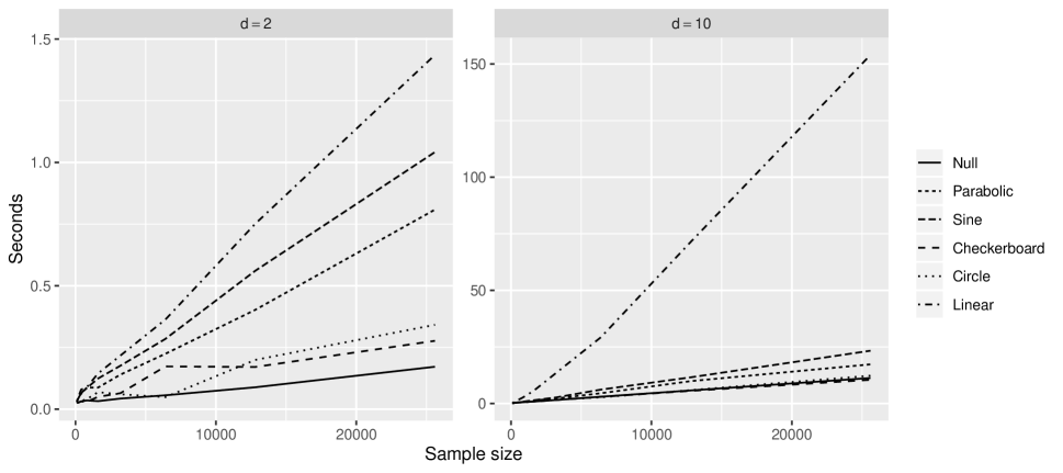
Figure S5: Computational scalability: run-time vs. sample size for the six simulation scenarios from Table S1 when fitted with MultiFIT in different dimensionalities with $D_{x}=D_{y}=d$, $R^{*}=1$ and $l=3$. In all cases the “linear” scenario requires the most computations and the “null” scenario the least.

We apply these methods to data sets simulated under six scenarios described in Table S1 along with a “null” scenario where there is no dependence. Here we report the results for two scenarios as they represent the best- and worst-case computational scenarios for MultiFIT and defer the rest of the scenarios to Figure S5 in the Supplementary Materials. The first scenario we report involves data generated under the null hypothesis, with all margins being drawn independently from a standard normal distribution. Under the second scenario, one dimension of $\mathbf{Y}$ is strongly correlated with a dimension of $\mathbf{X}$ under the “linear” scenario from Table S1 with $l=3$. While in practice non-linear alternatives are the main motivation for the nonparametric tests being considered here, the linear scenario is essentially the worst-case scenario for MultiFIT in terms of computational time. The reason is that the stronger the dependency at coarser levels, the more tests will be performed under MultiFIT because more tests will pass the $p$-value threshold at coarser levels. As such, these two scenarios represent the two ends of the spectrum in the amount of computation incurred under MultiFIT.

Figure 6 plots the computational time versus the sample size ( in log-log scale) at different dimensionalities—2 and 10. All methods were run on the same desktop computer with a single Intel^® Core(TM) i7-3770 CPU unit at 3.40GHz, and the three competitors were evaluated up to the maximum sample size allowed by the available 16G RAM. We present the average duration of 10 executions of each method under different dimensions, $d=2$ and $d=10$. It is worth noting that the results for the competitors are for only a single permutation while at least hundreds of resampling repetitions are required in order to perform inference.

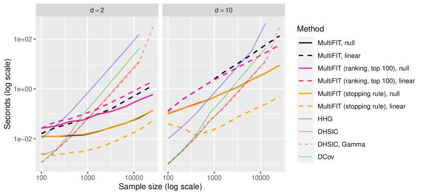
Figure 6: Computational scalability: a comparison of HHG, DCov, dHSIC (a single computation of the test statistic) and MultiFIT with $D_{x}=D_{y}=d$, log runtime versus log sample size. MultiFIT was run with $R^{*}=1$ and $p^{*}=(D_{x}\cdot D_{y}\cdot\log_{2}(n))^{-1}$. Three variants of MultiFIT are investigated: the full algorithm, the approximate algorithm that keeps up to 100 most significant $p$-values at each resolution, and the full algorithm with early stopping. MultiFIT and dHSIC with Gamma approximation does not require permutation. The other methods require permutations for level control and the reported time is for a single permutation

.

Overall, the computational advantage MultiFIT is substantial—it scales approximately $O(n\log n)$ in sample size, while HHG, DCov and dHSIC without the Gamma approximation scale approximately $O(n^{2})$. The Gamma approximation method of dHSIC makes the method faster in the presence of a strong signal, but it still cannot handle the larger sample sizes due to its memory requirement. MultiFIT with early stopping achieved the best computational efficiency at moderate to large sample sizes uniformly across non-null scenarios. As expected, early stopping does not reduce computation under the null. The approximate MultiFIT with a maximum number of cuboids per resolution on the other hand bounds the complexity by $O(n\log n)$.

We do acknowldge that the three competitors scale linearly in dimensionality while MultiFIT scales quadratically with the number of dimensions. As such MultiFIT is not suited for very high-dimensional problems. It is most suitable for problems up to tens of dimensions with large sample size.

3.2 Power Comparison

We next examine the statistical power of the competing methods under several representative dependency scenarios. We consider two sets of simulation settings. In one set, the dependency exists only in a small number of margins, and thus is amenable to MultiFIT’s search over pairs of axes-aligned boundaries. In the other set, the dependency is spread over a large number of dimensions and thus is particularly adversarial to MultiFIT.

In the first set of simulations, we let $X_{1}$ and $Y_{1}$ be independently normally distributed, whereas $X_{2}$ and $Y_{2}$ are dependent according to several different scenarios, which are illustrated in Figure 7 in black points in the upper row of plots and detailed in Table S1. MultiFIT has a natural advantage to detect such marginal dependencies as it focuses on the testing of pairs of margins.

In the second set of dependency scenarios, the true signal embodies dependencies of the $Y$ margins on multiple $X$ margins in terms of linear combinations or mixtures. This dissipates the strength of the dependency over many pairs of margins and thus is highly unfavorable to MultiFIT. This set of scenarios is illustrated in Figure 7 in green points in the two rows of plots and detailed in Table S2 and Table S3.

For all scenarios except the “local” scenarios, we set the level of resolutions up to which exhaustive testing is done, $R^{*}=2$, and for the “local” scenarios, where a signal is embedded in a small portion of the sample space, we set $R^{*}=4$ to ensure exhaustive coverage up to resolution 4. In Section S6 we present a detailed sensitivity analysis on the effects of the tuning parameters $p^{*}$ and $R^{*}$ on the power of the test under the simulation settings.

We performed 500 simulations for each scenario and at 20 different noise levels, and applied the four methods at the 5% level. We first applied a rank transform to each of the $D$ margins for the simulated data as this is the default under MultiFIT and the competitors HHG, DCov and dHSIC also performed much better with the marginal rank transform.

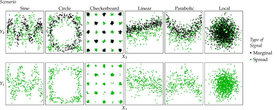
Figure 7: Visualization of the dependent margins of six scenarios with noise level 2. Note that the black, “marginal” scenario is only plotted in the top row as its $X_{1}$-$Y_{1}$ margins do not involve an interesting dependency, whereas the “spread” scenario is plotted in both. The dependency in the marginal scenario is more noticeable in the $X_{2}$-$Y_{2}$ margins than the spread scenario.

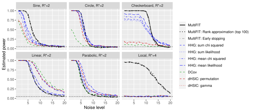
Figure 8: Power versus noise level for different methods. Estimated power at 20 noise levels for the different methods under the six scenarios from Table S1.

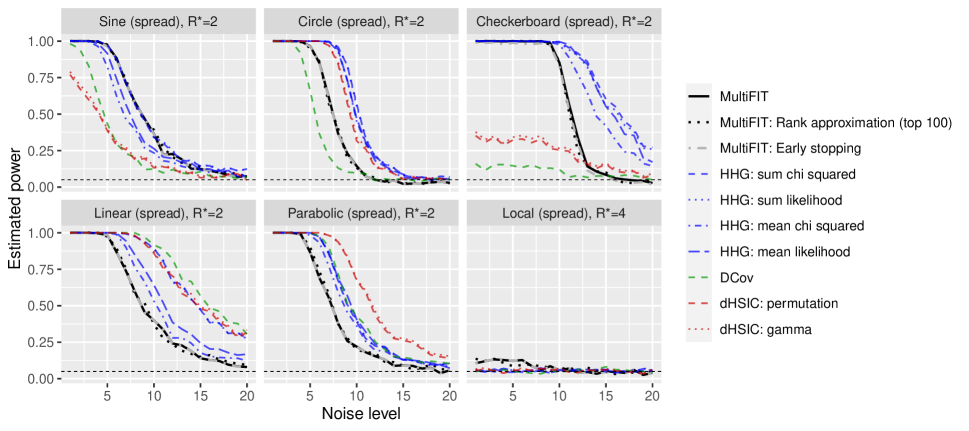
Figure 9: Power versus noise level for different methods. Estimated power at 20 noise levels for the different methods under the six scenarios from Table S2 and Table S3.

Figure 8 reports the result for the first set of simulations. MultiFIT outperforms HHG, DCov and dHSIC for the “sine”, “circle”, “checkerboard” and “local” scenarios, the cases that are richer with local structures. For the more “global” dependency structures—“linear” and “parabolic”— HHG and dHSIC outperform MultiFIT, while DCov does so only in the “linear” case. This is explained by the fact that the signal is observable almost entirely in the coarsest level, and as we go into higher resolutions we merely add insignificant tests that reduce the overall power. In the second set of simulations (Figure 9), as expected, MultiFIT loses some power relative to the competitors. Nevertheless, its overall performance is still robust and it still outperforms all other methods in the “sine” and “local” spread scenarios.

The results are largely consistent with our intuition. Due to its divide-and-conquer nature, MultiFIT is particularly good a identifying dependency structures that concentrates within a small number of cuboids (i.e., local features), while its power is weaker when the dependency structure is spread over a large number of cuboids (i.e., global structures).

Finally, we acknowledg that the performance of some of the competitors, such as HSIC, could be further improved with more expert selection of tuning parameters. For example, the incorporation of a multi-scale bandwidth into HSIC (Li and Yuan,, 2019) could further improve its performance.

3.3 Learning the nature of the dependency

So far we have focused on applying MultiFIT for testing the null hypothesis of independence. In practice, especially in multivariate settings, the practitioner is often interested in not just testing the existence of dependence but to have an understanding of its nature. A by-product of the divide-and-conquer approach is the ability to shed light on the underlying dependency structure. In this section we provide two examples that illustrate MultiFIT’s ability of learning the nature of the dependency. In the first example we consider a dependency structure resulting from higher order interactions. In the second example the dependency consists of two sine waves in the $(X_{1},Y_{1})$ margin with different frequencies, while a third margin, $X_{2}$, determines the frequency. In both examples it is difficult to visualize the dependency in low-dimensional marginal visualizations. We show that after identifying the $2\times 2$ tables that contained statistically significant evidence for dependency (after multiple testing correction), by plotting the data points in those significant tables, one can learn and visualize the underlying dependency. In both examples, we use the holistic approach to multiple testing and adopt Holm’s correction on the $p$-values.

3.3.1 Example 1: Rotated 3D Circle

Let $\mathbf{X}$ and $\mathbf{Y}$ each be of three dimensions, and simulate a sample with 800 observations. We first generate a “circle” scenario so that $X_{1}$, $Y_{1}$, $X_{2}$, and $Y_{2}$ are all i.i.d. standard normals, whereas $X_{3}=\cos(\theta)+\epsilon$, $Y_{3}=\sin(\theta)+\epsilon^{\prime}$ where $\epsilon$ and $\epsilon^{\prime}$ are i.i.d $\mathrm{N}(0,(1/10)^{2})$ and $\theta\sim\mathrm{Uniform}(-\pi,\pi)$. We then rotate the circle by $\pi/4$ degrees in the $X_{2}$-$X_{3}$-$Y_{3}$ space by applying:

$$\left[\begin{matrix}\cos(\pi/4)&-\sin(\pi/4)&0\\ \sin(\pi/4)&\cos(\pi/4)&0\\ 0&0&1\end{matrix}\right]\left[\begin{matrix}|&|&|\\ X_{2}&X_{3}&Y_{3}\\ |&|&|\end{matrix}\right].$$

The rotated circle is no longer visible by examining the 2-dimensional margins. See Figure 10 for the marginal views of the sample before and after the rotation. Figure 11 plots the data points that lie in the $2\times 2$ tables identified as statistical significant (at 0.001 level after multiple testing adjustment with modified Holm’s procedure) under the rotated setting. The underlying dependency pattern is clearly visible after selecting these tables. We found that in visualizing the identified tables, it is often useful to plot the data points that lie in the same slice of that table but with the full ranges of the plotted margins, as the identified table often captures a portion of the interesting dependency. Figure 11 demonstrates this technique by plotting those additional observations (in orange). For this reason, we have incorporated this plotting feature in our software.

(a)

(b)

Figure 10: Marginal views of the data sample in Section 3.3 (a) before and (b) after rotation. The dependency is easily visible in the marginal plots before rotation. Once rotated, the signal is spread among the margins and no longer visually obvious.

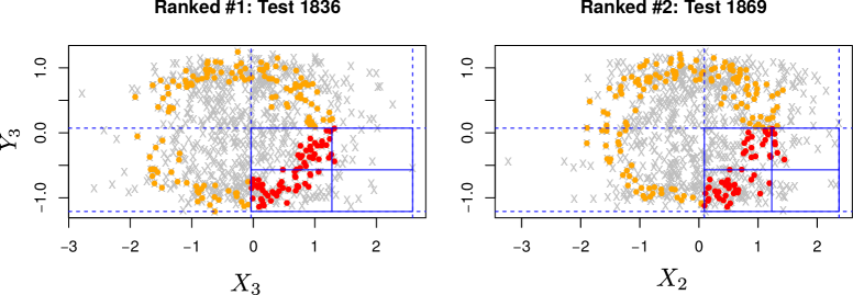
Figure 11: Scatter plots for the observations in the three $2\times 2$ tables identified as most significant by MultiFIT for the rotated circle scenario. (Significant tables are those with Holm’s adjusted $p$-values below 0.001.) The dependency structure is again visible in the marginal views: red points are observations that are within the cuboid that is tested, orange points are observations that are in a cuboid formed by expanding the tested cuboid so that the plotted margins are not subsetted. Notice how the left plot captures the dependency in the $X_{3}$-$Y_{3}$ plane while the right plot captures the dependency in the $X_{2}$-$Y_{3}$ plane.

3.3.2 Example 2: Mixed Sine Signals

Here we examine MultiFIT’s ability to detect a dependency structure consisting of two sine waves in different frequencies. Let $\mathbf{X}=(X_{1},X_{2})^{\prime}$ be a two-dimensional random vector with independent margins $X_{1}\sim U(0,1)$ and $X_{2}\sim Beta(0.3,0.3)$, and let

$$Y=\begin{cases}\sin(10\cdot X_{1})+\epsilon,&\text{if }X_{2}>0.5\\ \sin(40\cdot X_{1})+\epsilon,&\text{if }X_{2}\leq 0.5\end{cases}$$

Figure 12 shows a simulated dataset of size 800. In the $(X_{1},Y_{1})$ margin (the left panel) we can see the superimposed sine waves. Figure 13 shows three significant tables identified by MultiFIT using the same color coding technique from the previous example in which we can clearly discern between the different frequency waves.

Figure 12: The two pairs of margins of the sine mixture. In the left plot we see the superimposed sine signals, in the right plot the margins that determine the mixture.

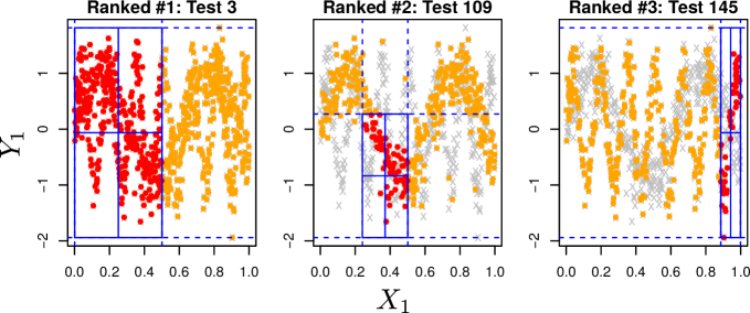
Figure 13: Scatter plots for the observations in the three $2\times 2$ tables identified as most significant by MultiFIT for the sine mixture scenario. The red points are observations that are within the cuboid that is tested, orange points are observations that are in a cuboid formed by expanding the tested cuboid so that the plotted margins are not subsetted.

4 Application to a flow cytometry data set

Flow cytometry is the standard biological assay used to measure single cell features known as markers, and is commonly used to quantify the relative frequencies of cell subsets in blood or disaggregated tissue. These features may be general physical, chemical or biological properties of a cell. Such data involve complex distributional features and are of massive sizes with typical sample sizes in the range of hundreds of thousands, which presents computational challenges to nonparametric data analytical tools.

For the evaluation, we used flow cytometry samples generated by an antibody panel designed to identify activated T cell subsets. We show the results of the dependency analysis on a single illustrative sample with 353,586 cells. For the analysis, we separated the markers into a vector of four ‘basic’ markers (dump, CD3, CD4, CD8) and a vector of four ‘functional’ markers (IFN, TNF, IL-2 and CD107). The basic markers are used in practice to first identify viable T cells by exclusion using the ‘dump’ and CD3 markers, and then to further partition T cells into CD4-positive (‘helper’) and CD8-positive (‘cytotoxic’) subsets. The functional markers are used to identify the activation status of these T cell subsets and their functional effector capabilities (IL-2 is a T cell growth factor, IFN and TNF are inflammatory cytokines, and CD107 is a component of the mechanism used by T cells to directly kill infected and cancer cells).

We applied MultiFIT with Holm’s multiple testing adjustment to the data to identifying dependency between the basic and functional markers. Our aim here is to demonstrate MultiFIT’s ability to handle such large data and to shed light on the underlying dependency, and so we ran the test exhaustively up to the maximal resolution of 4 - testing 102,416 $2\times 2$ tables. The execution time of the algorithm in this setting is approximately 5 minutes on a laptop computer utilizing four 3.00GHz Intel^® Xeon(R) E3-1505M v6 CPU cores.

As the sample size is very large and the data clearly have strong marginal dependencies, MultiFIT identified hundreds of significant tests after multiple testing adjustment. Interested readers can run our code for this example in the Supplementary Materials to visualize the identified dependence structures. None of HHG, DCov and dHSIC was able to handle this amount of data and all ended in overflow errors. Figure 14 presents the visualization of the observations in the 20 $2\times 2$ table with the most significant $p$-values using the strategy described in Section 3.3.

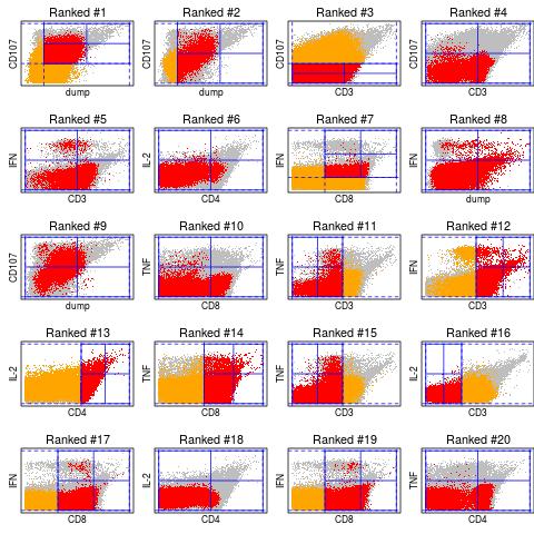
Figure 14: Scatter plots of the observations identified by the 20 $2\times 2$ tables with the most significant $p$-values for the flow cytometry data set. Red indicates observations in the tested cuboid. Orange indicates observations in the same slice of the sample space, determined by the four markers other than the two margins plotted. Gray indicates the rest of the observations.

5 Conclusion

We have presented a scalable framework called MultiFIT for nonparametrically testing the independence of random vectors that achieves high computational scalability, decent statistical power, and the ability to shed light on the underlying dependency. We provide a finite-sample theoretical guarantee that MultiFIT controls the level exactly at any finite sample size without resorting to resampling or asymptotic approximation. The proposed approach is most suitable for multivariate problems up to tens of dimensions, can scale up to massive sample sizes, and thus can be useful for many modern data analyses. We have published an R package called MultiFit on CRAN that implements the proposed method.

6 Software

For the MultiFIT procedure we used our R package MultiFit on CRAN. For the Heller-Heller-Gorfine (HHG) test (Heller et al.,, 2013) we used the HHG package on CRAN. For Distance Covariance (DCov) (Székely and Rizzo,, 2009) we used the energy package on CRAN. For dHSIC (Pfister et al.,, 2018) we used the dHSIC package on CRAN.

7 Acknowledgments

The authors wish to thank the editor, an AE, and two referees for their valuable comments and suggestions. LM’s research is partly supported by NSF grants DMS-1749789 and DMS-2013930. The flow cytometry data is collected through an EQAPOL collaboration with federal funds from the National Institute of Allergy and Infectious Diseases, National Institutes of Health, Contract Number HHSN272201700061C.

Supplementary Material

S1 Technical proofs

In this section, we establish proofs for Theorem 2.1, Theorem 2.2, and Corollary 2.1 in the main paper. We will introduce a number of definitions and lemmas along the way that will be used to complete the proofs.

Definition S1.1.

Level-$k$ Canonical Marginal Partition:
$\mathcal{P}^{k}$ is a level-$k$ canonical marginal partition if $\mathcal{P}^{k}=\left\{\left[\frac{l-1}{2^{k}},\frac{l}{2^{k}}\right)\right\}_{l\in\{1,...,2^{k}\}}.$

To simplify the notations in the proofs, we let $\bm{Z}=(\mathbf{X},\mathbf{Y})$. More specifically, we set $Z_{1}:=X_{1},...,Z_{D_{x}}:=X_{D_{x}}$ and $Z_{D_{x}+1}:=Y_{1},...,Z_{D}:=Y_{D_{y}}$. Thus, $\bm{Z}$ is a random vector that distributed according to the distribution $F$, the joint sampling distribution of $(\mathbf{X},\mathbf{Y})$.

For $\mathbf{k}=(k_{1},...,k_{D})\in\mathbb{N}_{0}^{D}$, we refer to the partition $\mathcal{P}^{k_{1}}\times\cdots\times\mathcal{P}^{k_{D}}$ as the $\mathbf{k}$-stratum of $\Omega$. Denote now any $\mathbf{k}$-stratum as $\mathcal{A}^{\mathbf{k}}$. As described in Section 2, we form $D$-dimensional cuboids by taking the Cartesian product of one interval from each of the $D$ canonical marginal partitions of $\Omega$. Given then $\mathbf{k}=(k_{1},...,k_{D})\in\mathbb{N}_{0}^{D}$ a specific cuboid is determined by some $\mathbf{l}=(l_{1},...,l_{D})$ with each $1\leq l_{d}\leq 2^{k_{d}}$ such that $A=\bigtimes_{d\in\{1,..,D\}}\left[\frac{l_{d}-1}{2^{k_{d}}},\frac{l_{d}}{2^{k_{d}}}\right)$. Figure S1 illustrates these definitions in a three dimensional space.

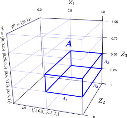
Figure S1: Cuboid and stratum.
A 3D view of a $\mathbf{k}$-stratum and the cuboid $A$ where $D=3$ and $\mathbf{k}=(1,0,2)$. The thin blue lines delineate all $(1,0,2)$-cuboids, that is, the stratum $\mathcal{A}^{(1,0,2)}=\mathcal{P}^{1}\times\mathcal{P}^{0}\times\mathcal{P}^{2}$. The thick blue lines delineate the cuboid $A$ for which $\mathbf{l}=(2,1,2)$, i.e., $A=A_{1}\times A_{2}\times A_{3}$ where $A_{1}=\left[\frac{2-1}{2^{1}},\frac{2}{2^{1}}\right)=[0.5,1)\in\mathcal{P}^{1}$, $A_{2}=\left[\frac{1-1}{2^{0}},\frac{1}{2^{0}}\right)=[0,1)\in\mathcal{P}^{0}$, and $A_{3}=\left[\frac{2-1}{2^{2}},\frac{2}{2^{2}}\right)=[0.25,0.5)\in\mathcal{P}^{2}$. The resolution of this stratum is $3=1+0+2$.

We next define a discretized form of independence which we will show in Lemma S1.1 fully characterizes the multivariate independence:

Definition S1.2.

$\mathbf{k}$-independence:
For any $A\in\mathcal{A}^{\mathbf{k}}$, we can write $A=A_{x}\times A_{y}$ where

$$A_{x}=\bigtimes_{d=1}^{D_{x}}\left[\frac{l_{d}-1}{2^{k_{d}}},\frac{l_{d}}{2^{k_{d}}}\right)\text{ and }A_{y}=\bigtimes_{d=D_{x}+1}^{D}\left[\frac{l_{d}-1}{2^{k_{d}}},\frac{l_{d}}{2^{k_{d}}}\right).$$

(Figure S2 illustrates the above notations in three dimensional space.)

We say that $\mathbf{X}$ and $\mathbf{Y}$ are $\mathbf{k}$-independent and write it as $\mathbf{X}\mathchoice{\mathrel{\hbox to0.0pt{$\displaystyle\perp$\hss}\mkern 2.0mu{\displaystyle\perp}}_{\mathbf{k}}}{\mathrel{\hbox to0.0pt{$\textstyle\perp$\hss}\mkern 2.0mu{\textstyle\perp}}_{\mathbf{k}}}{\mathrel{\hbox to0.0pt{$\scriptstyle\perp$\hss}\mkern 2.0mu{\scriptstyle\perp}}_{\mathbf{k}}}{\mathrel{\hbox to0.0pt{$\scriptscriptstyle\perp$\hss}\mkern 2.0mu{\scriptscriptstyle\perp}}_{\mathbf{k}}}\mathbf{Y}$ if for any $A\in\mathcal{A}^{\mathbf{k}}$,

$$\operatorname{P}\left(\mathbf{X}\in A_{x},\mathbf{Y}\in A_{y}\right)=\operatorname{P}\left(\mathbf{X}\in A_{x}\right)\cdot\operatorname{P}\left(\mathbf{Y}\in A_{y}\right).$$

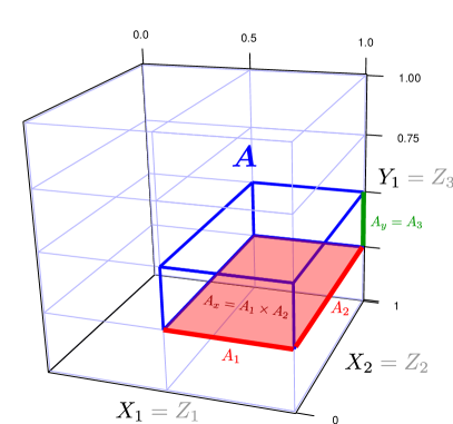
Figure S2: $A_{x}$ and $A_{y}$.
A 3D view of a $\mathbf{k}$-stratum and the cuboid $A$ where $D=3$, $\mathbf{k}=(1,0,2)$ and $\mathbf{l}=(2,1,2)$, the same as in Figure S1. Here $D_{x}=2$ with $X_{1}=Z_{1}$ and $X_{2}=Z_{2}$; $D_{y}=1$ with $Y_{1}=Z_{3}$. The cuboid $A$ is represented now as $A=A_{x}\times A_{y}$ where $A_{x}=A_{1}\times A_{2}=\left[\frac{2-1}{2^{1}},\frac{2}{2^{1}}\right)\times\left[\frac{1-1}{2^{0}},\frac{1}{2^{0}}\right)=[0.5,1)\times[0,1)$, and $A_{y}=A_{3}=\left[\frac{2-1}{2^{2}},\frac{2}{2^{2}}\right)=[0.25,0.5)$.

Definition S1.3.

$(i,j)$-blocks of a cuboid:
For every cuboid $A\in\mathcal{A}^{\mathbf{k}}$, $i\in\{1,..,D_{x}\}$ and $j\in\{1,..,D_{y}\}$, one can partition $A$ into four blocks by dividing $A$ in the $(i,j)$th face (that is, the side of $A$ spanned by the $i$th and $j$th dimensions) while keeping the other dimensions intact.

$$A=A_{ij}^{00}\cup A_{ij}^{01}\cup A_{ij}^{10}\cup A_{ij}^{11},$$

where for $a,b\in\{0,1\}$,

$$A_{ij}^{ab}=\bigtimes_{d=1}^{D}\begin{cases}\left[\frac{2l_{d}-2+a}{2^{k_{\!d}+1}},\frac{2l_{d}-1+a}{2^{k_{\!d}+1}}\right)&\text{if }d=i\\ \left[\frac{2l_{d}-2+b}{2^{k_{\!d}+1}},\frac{2l_{d}-1+b}{2^{k_{\!d}+1}}\right)&\text{if }d=D_{x}+j\\ \left[\frac{l_{d}-1}{2^{k_{\!d}}},\frac{l_{d}}{2^{k_{\!d}}}\right)&\text{if }d\in\{1,..,D\}\setminus\{i,D_{x}+j\}\\ \end{cases}.$$

Figure S3 illustrates Definition S1.3 in three dimensions.

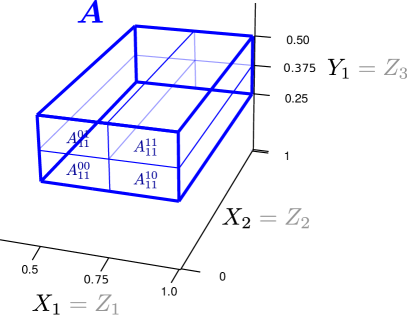
Figure S3: ($i=1$, $j=1$) blocks of $A$.
A 3D view of the $\mathbf{k}$-cuboid $A$ where $D=3$, $\mathbf{k}=(1,0,2)$ and $\mathbf{l}=(2,1,2)$, the same as in Figures S1 and S2. Note that the $i=1$ dimension of $\mathbf{X}$ corresponds to dimension 1 of $\bm{Z}$ the $j=1$ dimension of $\mathbf{Y}$ corresponds to dimension 3 of $\bm{Z}$. The blocks are:
$A_{11}^{00}=\left[\frac{2\cdot 2-2+0}{2^{1+1}},\frac{2\cdot 2-1+0}{2^{1+1}}\right)\times\left[\frac{1-1}{2^{0}},\frac{1}{2^{0}}\right)\times\left[\frac{2\cdot 2-2+0}{2^{2+1}},\frac{2\cdot 2-1+0}{2^{2+1}}\right)=[0.5,0.75)\times[0,1)\times[0.25,0.375)$,
$A_{11}^{01}=\left[\frac{2\cdot 2-2+0}{2^{1+1}},\frac{2\cdot 2-1+0}{2^{1+1}}\right)\times\left[\frac{1-1}{2^{0}},\frac{1}{2^{0}}\right)\times\left[\frac{2\cdot 2-2+1}{2^{2+1}},\frac{2\cdot 2-1+1}{2^{2+1}}\right)=[0.5,0.75)\times[0,1)\times[0.375,0.5)$,
$A_{11}^{10}=\left[\frac{2\cdot 2-2+1}{2^{1+1}},\frac{2\cdot 2-1+1}{2^{1+1}}\right)\times\left[\frac{1-1}{2^{0}},\frac{1}{2^{0}}\right)\times\left[\frac{2\cdot 2-2+0}{2^{2+1}},\frac{2\cdot 2-1+0}{2^{2+1}}\right)=[0.75,1)\times[0,1)\times[0.25,0.375)$,
$A_{11}^{11}=\left[\frac{2\cdot 2-2+1}{2^{1+1}},\frac{2\cdot 2-1+1}{2^{1+1}}\right)\times\left[\frac{1-1}{2^{0}},\frac{1}{2^{0}}\right)\times\left[\frac{2\cdot 2-2+1}{2^{2+1}},\frac{2\cdot 2-1+1}{2^{2+1}}\right)=[0.75,1)\times[0,1)\times[0.375,0.5)$.

Lemma S1.1 establishes an equivalence between multivariate independence and a cascade of discretized multivariate independence relations:

Lemma S1.1.

$$\mathbf{X}\mathchoice{\mathrel{\hbox to0.0pt{$\displaystyle\perp$\hss}\mkern 2.0mu{\displaystyle\perp}}}{\mathrel{\hbox to0.0pt{$\textstyle\perp$\hss}\mkern 2.0mu{\textstyle\perp}}}{\mathrel{\hbox to0.0pt{$\scriptstyle\perp$\hss}\mkern 2.0mu{\scriptstyle\perp}}}{\mathrel{\hbox to0.0pt{$\scriptscriptstyle\perp$\hss}\mkern 2.0mu{\scriptscriptstyle\perp}}}\mathbf{Y}\hskip 6.0pt\Leftrightarrow\hskip 6.0pt\mathbf{X}\mathchoice{\mathrel{\hbox to0.0pt{$\displaystyle\perp$\hss}\mkern 2.0mu{\displaystyle\perp}}_{\mathbf{k}}}{\mathrel{\hbox to0.0pt{$\textstyle\perp$\hss}\mkern 2.0mu{\textstyle\perp}}_{\mathbf{k}}}{\mathrel{\hbox to0.0pt{$\scriptstyle\perp$\hss}\mkern 2.0mu{\scriptstyle\perp}}_{\mathbf{k}}}{\mathrel{\hbox to0.0pt{$\scriptscriptstyle\perp$\hss}\mkern 2.0mu{\scriptscriptstyle\perp}}_{\mathbf{k}}}\mathbf{Y}\quad\text{for all $\mathbf{k}\in\mathbb{N}_{0}^{D}$}.$$

Proof.

$\Rightarrow$: Immediate.
$\Leftarrow$:
Let $\mathcal{P}_{x}=\bigcup_{\mathbf{k}_{\{1,\ldots D_{x}\}}\in\mathbb{N}_{0}^{D_{x}}}\mathcal{P}^{1}\times\ldots\mathcal{P}^{D_{x}}$. Therefore $\sigma(\mathcal{P}_{x})=\mathcal{B}([0,1]^{D_{x}})$.
For $A_{x}\in\mathcal{B}([0,1]^{D_{x}})$ let $[\mathbf{X}\in A_{x}]=\{\bm{\omega}:\mathbf{X}(\bm{\omega})\in A_{x}\}$, then $\sigma(\mathbf{X})=\{[\mathbf{X}\in A_{x}],A_{x}\in\mathcal{B}([0,1]^{D_{x}})\}$.
Let $\mathcal{Q}_{x}=\bigcup_{\mathbf{k}_{\{1,\ldots D_{x}\}}\in\{-1,0,1,2,...\}^{D_{x}}}\mathcal{Q}^{k_{1}}\times...\times\mathcal{Q}^{k_{D_{x}}}$ so that $\mathcal{Q}^{-1}:=\emptyset$ and $\forall k\geq 0$, $\mathcal{Q}^{k}=\mathcal{P}^{k}$.

Let $\mathcal{C}_{\mathbf{X}}=\{[\mathbf{X}\in B_{x}],B_{x}\in\mathcal{Q}_{x}\}$.

Hence $\sigma(\mathcal{C}_{\mathbf{X}})=\sigma(\mathbf{X}^{-1}(B_{x}),B_{x}\in\mathcal{Q}_{x})=\sigma(\mathbf{X}^{-1}(\mathcal{Q}_{x}))=\mathbf{X}^{-1}(\sigma(\mathcal{Q}_{x}))=\mathbf{X}^{-1}(\sigma(\mathcal{P}_{x}))=\sigma(\mathbf{X})$.
Note that $\mathcal{C}_{\mathbf{X}}$ is a $\pi$-system:
$E,E^{\prime}\in\mathcal{C}_{\mathbf{X}}\hskip 6.0pt\Rightarrow\hskip 6.0ptE=\left[\mathbf{X}\in\left(\emptyset\text{ or }\left[\frac{l_{1}-1}{2^{k_{1}}},\frac{l_{1}}{2^{k_{1}}}\right)\right)\times\ldots\times\left(\emptyset\text{ or }\left[\frac{l_{D_{x}}-1}{2^{k_{D_{x}}}},\frac{l_{D_{x}}}{2^{k_{D_{x}}}}\right)\right)\right]$ and
$E^{\prime}=\left[\mathbf{X}\in\left(\emptyset\text{ or }\left[\frac{l^{\prime}_{1}-1}{2^{k^{\prime}_{1}}},\frac{l^{\prime}_{1}}{2^{k^{\prime}_{1}}}\right)\right)\times\ldots\times\left(\emptyset\text{ or }\left[\frac{l^{\prime}_{D_{x}}-1}{2^{k^{\prime}_{D_{x}}}},\frac{l^{\prime}_{D_{x}}}{2^{k^{\prime}_{D_{x}}}}\right)\right)\right]$ for some $\mathbf{l},\mathbf{l}^{\prime},\mathbf{k},\mathbf{k}^{\prime}$. Therefore:

$$E\cap E^{\prime} =\left[\mathbf{X}\in\left\{\left(\emptyset\text{ or }\left[\frac{l_{1}-1}{2^{k_{1}}},\frac{l_{1}}{2^{k_{1}}}\right)\right)\times\ldots\times\left(\emptyset\text{ or }\left[\frac{l_{D_{x}}-1}{2^{k_{D_{x}}}},\frac{l_{D_{x}}}{2^{k_{D_{x}}}}\right)\right)\right\}\right.\bigcap$$

$$\hskip 60.0pt\left.\left\{\left(\emptyset\text{ or }\left[\frac{l^{\prime}_{1}-1}{2^{k^{\prime}_{1}}},\frac{l^{\prime}_{1}}{2^{k^{\prime}_{1}}}\right)\right)\times\ldots\times\left(\emptyset\text{ or }\left[\frac{l^{\prime}_{D_{x}}-1}{2^{k^{\prime}_{D_{x}}}},\frac{l^{\prime}_{D_{x}}}{2^{k^{\prime}_{D_{x}}}}\right)\right)\right\}\right]$$

$$=\left[\mathbf{X}\in\left(\emptyset\text{ or }\left[\frac{l_{1}-1}{2^{k_{1}}},\frac{l_{1}}{2^{k_{1}}}\right)\cap\left[\frac{l^{\prime}_{1}-1}{2^{k^{\prime}_{1}}},\frac{l^{\prime}_{1}}{2^{k^{\prime}_{1}}}\right)\right)\times\ldots\right.$$

$$\hskip 60.0pt\left.\times\left(\left[\frac{l_{D_{x}}-1}{2^{k_{D_{x}}}},\frac{l_{D_{x}}}{2^{k_{D_{x}}}}\right)\cap\left[\frac{l^{\prime}_{D_{x}}-1}{2^{k^{\prime}_{D_{x}}}},\frac{l^{\prime}_{D_{x}}}{2^{k^{\prime}_{D_{x}}}}\right)\right)\right]\in\mathcal{C}_{\mathbf{X}}$$

Similarly, define $\sigma(\mathbf{Y})$ and $\mathcal{C}_{\mathbf{Y}}$, another $\pi$-system, independent of $\mathcal{C}_{\mathbf{X}}$ and $\sigma(\mathbf{Y})=\sigma(\mathcal{C}_{\mathbf{Y}})$. By the basic criterion, then, $\sigma(\mathbf{X})\mathchoice{\mathrel{\hbox to0.0pt{$\displaystyle\perp$\hss}\mkern 2.0mu{\displaystyle\perp}}}{\mathrel{\hbox to0.0pt{$\textstyle\perp$\hss}\mkern 2.0mu{\textstyle\perp}}}{\mathrel{\hbox to0.0pt{$\scriptstyle\perp$\hss}\mkern 2.0mu{\scriptstyle\perp}}}{\mathrel{\hbox to0.0pt{$\scriptscriptstyle\perp$\hss}\mkern 2.0mu{\scriptscriptstyle\perp}}}\sigma(\mathbf{Y})$. ∎

The following lemma shows that if $\mathbf{X}$ and $\mathbf{Y}$ are $\mathbf{k}$-independent, they are also independent on all coarser strata.

Lemma S1.2.

If $\mathbf{X}\mathchoice{\mathrel{\hbox to0.0pt{$\displaystyle\perp$\hss}\mkern 2.0mu{\displaystyle\perp}}_{\mathbf{k}}}{\mathrel{\hbox to0.0pt{$\textstyle\perp$\hss}\mkern 2.0mu{\textstyle\perp}}_{\mathbf{k}}}{\mathrel{\hbox to0.0pt{$\scriptstyle\perp$\hss}\mkern 2.0mu{\scriptstyle\perp}}_{\mathbf{k}}}{\mathrel{\hbox to0.0pt{$\scriptscriptstyle\perp$\hss}\mkern 2.0mu{\scriptscriptstyle\perp}}_{\mathbf{k}}}\mathbf{Y}$ then $\mathbf{X}\mathchoice{\mathrel{\hbox to0.0pt{$\displaystyle\perp$\hss}\mkern 2.0mu{\displaystyle\perp}}_{\mathbf{k}^{\prime}}}{\mathrel{\hbox to0.0pt{$\textstyle\perp$\hss}\mkern 2.0mu{\textstyle\perp}}_{\mathbf{k}^{\prime}}}{\mathrel{\hbox to0.0pt{$\scriptstyle\perp$\hss}\mkern 2.0mu{\scriptstyle\perp}}_{\mathbf{k}^{\prime}}}{\mathrel{\hbox to0.0pt{$\scriptscriptstyle\perp$\hss}\mkern 2.0mu{\scriptscriptstyle\perp}}_{\mathbf{k}^{\prime}}}\mathbf{Y}$ for all $\mathbf{k}^{\prime}\leq\mathbf{k}$.

Proof.

Let $F_{\mathbf{X}}$ be the probability distribution of $\mathbf{X}$ and $F_{\mathbf{Y}}$ be the probability distribution of $\mathbf{Y}$. Then $\mathbf{X}\mathchoice{\mathrel{\hbox to0.0pt{$\displaystyle\perp$\hss}\mkern 2.0mu{\displaystyle\perp}}_{\mathbf{k}}}{\mathrel{\hbox to0.0pt{$\textstyle\perp$\hss}\mkern 2.0mu{\textstyle\perp}}_{\mathbf{k}}}{\mathrel{\hbox to0.0pt{$\scriptstyle\perp$\hss}\mkern 2.0mu{\scriptstyle\perp}}_{\mathbf{k}}}{\mathrel{\hbox to0.0pt{$\scriptscriptstyle\perp$\hss}\mkern 2.0mu{\scriptscriptstyle\perp}}_{\mathbf{k}}}\mathbf{Y}\hskip 6.0pt\Leftrightarrow\hskip 6.0ptF(A)=F_{\mathbf{X}}(A_{x})F_{\mathbf{Y}}(A_{y})$ for all $A\in\mathcal{A}^{\mathbf{k}}$.

It is enough to show that $\mathbf{X}\mathchoice{\mathrel{\hbox to0.0pt{$\displaystyle\perp$\hss}\mkern 2.0mu{\displaystyle\perp}}_{\mathbf{k}}}{\mathrel{\hbox to0.0pt{$\textstyle\perp$\hss}\mkern 2.0mu{\textstyle\perp}}_{\mathbf{k}}}{\mathrel{\hbox to0.0pt{$\scriptstyle\perp$\hss}\mkern 2.0mu{\scriptstyle\perp}}_{\mathbf{k}}}{\mathrel{\hbox to0.0pt{$\scriptscriptstyle\perp$\hss}\mkern 2.0mu{\scriptscriptstyle\perp}}_{\mathbf{k}}}\mathbf{Y}\hskip 6.0pt\Rightarrow\hskip 6.0pt\mathbf{X}\mathchoice{\mathrel{\hbox to0.0pt{$\displaystyle\perp$\hss}\mkern 2.0mu{\displaystyle\perp}}_{\mathbf{k}^{\prime}}}{\mathrel{\hbox to0.0pt{$\textstyle\perp$\hss}\mkern 2.0mu{\textstyle\perp}}_{\mathbf{k}^{\prime}}}{\mathrel{\hbox to0.0pt{$\scriptstyle\perp$\hss}\mkern 2.0mu{\scriptstyle\perp}}_{\mathbf{k}^{\prime}}}{\mathrel{\hbox to0.0pt{$\scriptscriptstyle\perp$\hss}\mkern 2.0mu{\scriptscriptstyle\perp}}_{\mathbf{k}^{\prime}}}\mathbf{Y}$ for any $\mathbf{k}^{\prime}$ such that (i) $k^{\prime}_{i}=k_{i}-1$ for some $i\in\{1,...,D_{x}\}$ and (ii) $k^{\prime}_{d}=k_{d}$ for all $d\in\{1,..,D\}\setminus\{i\}$.

Hence, assuming $\mathbf{X}\mathchoice{\mathrel{\hbox to0.0pt{$\displaystyle\perp$\hss}\mkern 2.0mu{\displaystyle\perp}}_{\mathbf{k}}}{\mathrel{\hbox to0.0pt{$\textstyle\perp$\hss}\mkern 2.0mu{\textstyle\perp}}_{\mathbf{k}}}{\mathrel{\hbox to0.0pt{$\scriptstyle\perp$\hss}\mkern 2.0mu{\scriptstyle\perp}}_{\mathbf{k}}}{\mathrel{\hbox to0.0pt{$\scriptscriptstyle\perp$\hss}\mkern 2.0mu{\scriptscriptstyle\perp}}_{\mathbf{k}}}\mathbf{Y}$ we get for $A\in\mathcal{A}^{\mathbf{k}^{\prime}}$ that:

$$F\left(A\right) =F\left(A_{1}\times...\times A_{i-1}\times A_{i}^{0}\times A_{i+1}\times...\times A_{D_{x}}\times A_{y}\right)$$

$$\hskip 12.0pt+F\left(A_{1}\times...\times A_{i-1}\times A_{i}^{1}\times A_{i+1}\times...\times A_{D_{x}}\times A_{y}\right)$$

$$=F_{\mathbf{X}}\left(A_{1}\times...\times A_{i-1}\times A_{i}^{0}\times A_{i+1}\times...\times A_{D_{x}}\right)F_{\mathbf{Y}}(A_{y})$$

$$\hskip 12.0pt+F_{\mathbf{X}}\left(A_{1}\times...\times A_{i-1}\times A_{i}^{1}\times A_{i+1}\times...\times A_{D_{x}}\right)F_{\mathbf{Y}}(A_{y})$$

$$=F_{\mathbf{X}}\left(A_{x}\right)F_{\mathbf{Y}}(A_{y})$$

As required. ∎

In Lemma S1.6 we will show how to characterize the multivariate $\mathbf{k}$-independence with a collection of univariate $(i,j)$ odds-ratios. However, before we state and prove Lemma S1.6 we develop additional notations and provide discretized versions of some basic results in probability. Denote:

$\mathbf{d}\subset\{1,..,D\}$, $\mathbf{i}=\mathbf{d}\cap\{1,..,D_{x}\}$ and $\mathbf{j}=\left\{j:j+D_{x}\in\mathbf{d}\cap\{D_{x}+1,...,D\}\right\}$
And

$$\mathbf{X}_{\mathbf{i}} =\{X_{i}:i\in\mathbf{i}\}, \mathbf{X}_{(\mathbf{i})} =\{X_{i^{\prime}}:i^{\prime}\in\{1,..,D_{x}\}\setminus\mathbf{i}\}$$

$$\mathbf{Y}_{\mathbf{j}} =\{Y_{j}:j\in\mathbf{j}\}, \mathbf{Y}_{(\mathbf{j})} =\{Y_{j^{\prime}}:j^{\prime}\in\{1,..,D_{y}\}\setminus\mathbf{j}\}$$

$$\bm{Z}_{\mathbf{d}} =\mathbf{X}_{\mathbf{i}}\times\mathbf{Y}_{\mathbf{j}}=\{Z_{d}:d\in\mathbf{d}\}, \bm{Z}_{(\mathbf{d})} =\mathbf{X}_{(\mathbf{i})}\times\mathbf{Y}_{(\mathbf{j})}=\{Z_{d^{\prime}}:d^{\prime}\in\{1,..,D\}\setminus\mathbf{d}\}$$

$$A_{x,\mathbf{d}} =\bigtimes_{d\in\mathbf{d}\cap\{1,..,D_{x}\}}A_{d}, A_{x,(\mathbf{d})} =\bigtimes_{d^{\prime}\in\{1,..,D_{x}\}\setminus\mathbf{d}}A_{d^{\prime}}$$

$$A_{y,\mathbf{d}} =\bigtimes_{d\in\mathbf{d}\cap\{D_{x}+1,..,D\}}A_{d}, A_{y,(\mathbf{d})} =\bigtimes_{d^{\prime}\in\{D_{x}+1,..,D\}\setminus\mathbf{d}}A_{d^{\prime}}$$

$$A_{\mathbf{d}} =A_{x,\mathbf{d}}\times A_{y,\mathbf{d}}=\bigtimes_{d\in\mathbf{d}}A_{d}, A_{(\mathbf{d})} =A_{x,(\mathbf{d})}\times A_{y,(\mathbf{d})}=\bigtimes_{d^{\prime}\in\{1,..,D\}\setminus\mathbf{d}}A_{d^{\prime}}$$

$$\mathbf{k}_{\mathbf{d}}=\{k_{d}:d\in\mathbf{d}\},\quad\quad\mathbf{k}_{(\mathbf{d})}=\{k_{d^{\prime}}:d^{\prime}\in\{1,..,D\}\setminus\mathbf{d}\}$$

Definition S1.4.

Conditional $\mathbf{k}$-independence:
We say that $\mathbf{X}_{\mathbf{i}}$ and $\mathbf{Y}_{\mathbf{j}}$ are $\mathbf{k}$-independent conditional on $\bm{Z}_{(\mathbf{d})}$ and write it as $\mathbf{X}_{\mathbf{i}}\mathchoice{\mathrel{\hbox to0.0pt{$\displaystyle\perp$\hss}\mkern 2.0mu{\displaystyle\perp}}_{\mathbf{k}}}{\mathrel{\hbox to0.0pt{$\textstyle\perp$\hss}\mkern 2.0mu{\textstyle\perp}}_{\mathbf{k}}}{\mathrel{\hbox to0.0pt{$\scriptstyle\perp$\hss}\mkern 2.0mu{\scriptstyle\perp}}_{\mathbf{k}}}{\mathrel{\hbox to0.0pt{$\scriptscriptstyle\perp$\hss}\mkern 2.0mu{\scriptscriptstyle\perp}}_{\mathbf{k}}}\mathbf{Y}_{\mathbf{j}}\mid\bm{Z}_{(\mathbf{d})}$ if for any $A\in\mathcal{A}^{\mathbf{k}}$:

$$\operatorname{P}\huge(\mathbf{X}_{\mathbf{i}}\in A_{x,\mathbf{d}}, \mathbf{Y}_{\mathbf{j}}\in A_{y,\mathbf{d}}\mid\bm{Z}_{(\mathbf{d})}\in A_{(\mathbf{d})}\huge)=\operatorname{P}\huge(\mathbf{X}_{\mathbf{i}}\in A_{x,\mathbf{d}}\mid\bm{Z}_{(\mathbf{d})}\in A_{(\mathbf{d})}\huge)\cdot\operatorname{P}\huge(\mathbf{Y}_{\mathbf{j}}\in A_{y,\mathbf{d}}\mid\bm{Z}_{(\mathbf{d})}\in A_{(\mathbf{d})}\huge)$$

Or equivalently:

$$\operatorname{P}\huge(\mathbf{X}_{\mathbf{i}}\in A_{x,\mathbf{d}} \mid\mathbf{Y}_{\mathbf{j}}\in A_{y,\mathbf{d}},\bm{Z}_{(\mathbf{d})}\in A_{(\mathbf{d})}\huge)=\operatorname{P}\huge(\mathbf{X}_{\mathbf{i}}\in A_{x,\mathbf{d}}\mid\bm{Z}_{(\mathbf{d})}\in A_{(\mathbf{d})}\huge)$$

When $k_{d^{\prime}}=0$ for some $d^{\prime}\in\{1,..,D\}\setminus\mathbf{d}$, $\Omega_{Z_{d^{\prime}}}=[0,1]$ for those indices and hence our notation may be compacted. For example, if $k_{d^{\prime}}=0$ for all $d^{\prime}\in\{1,..,D\}\setminus\mathbf{d}$:

$$\mathbf{X}_{\mathbf{i}}\mathchoice{\mathrel{\hbox to0.0pt{$\displaystyle\perp$\hss}\mkern 2.0mu{\displaystyle\perp}}_{\mathbf{k}}}{\mathrel{\hbox to0.0pt{$\textstyle\perp$\hss}\mkern 2.0mu{\textstyle\perp}}_{\mathbf{k}}}{\mathrel{\hbox to0.0pt{$\scriptstyle\perp$\hss}\mkern 2.0mu{\scriptstyle\perp}}_{\mathbf{k}}}{\mathrel{\hbox to0.0pt{$\scriptscriptstyle\perp$\hss}\mkern 2.0mu{\scriptscriptstyle\perp}}_{\mathbf{k}}}\mathbf{Y}_{\mathbf{j}}|\bm{Z}_{(\mathbf{d})}\hskip 6.0pt\Leftrightarrow\hskip 6.0pt\mathbf{X}_{\mathbf{i}}\mathchoice{\mathrel{\hbox to0.0pt{$\displaystyle\perp$\hss}\mkern 2.0mu{\displaystyle\perp}}_{\mathbf{k}_{\mathbf{d}}}}{\mathrel{\hbox to0.0pt{$\textstyle\perp$\hss}\mkern 2.0mu{\textstyle\perp}}_{\mathbf{k}_{\mathbf{d}}}}{\mathrel{\hbox to0.0pt{$\scriptstyle\perp$\hss}\mkern 2.0mu{\scriptstyle\perp}}_{\mathbf{k}_{\mathbf{d}}}}{\mathrel{\hbox to0.0pt{$\scriptscriptstyle\perp$\hss}\mkern 2.0mu{\scriptscriptstyle\perp}}_{\mathbf{k}_{\mathbf{d}}}}\mathbf{Y}_{\mathbf{j}}$$

We next provide a discretized version of some basic results in probability:

Lemma S1.3.

Contraction:
For $\mathbf{d}\subset\{1,..,D\}$ such that $\{1,..,D_{x}\}\subset\mathbf{d}$ (i.e. $\mathbf{i}=\{1,..,D_{x}\}$, $\mathbf{X}_{\mathbf{i}}=\mathbf{X}$ and $\mathbf{Y}_{(\mathbf{j})}=\bm{Z}_{(\mathbf{d})}$):

$$\begin{cases}\mathbf{X}\mathchoice{\mathrel{\hbox to0.0pt{$\displaystyle\perp$\hss}\mkern 2.0mu{\displaystyle\perp}}_{\mathbf{k}}}{\mathrel{\hbox to0.0pt{$\textstyle\perp$\hss}\mkern 2.0mu{\textstyle\perp}}_{\mathbf{k}}}{\mathrel{\hbox to0.0pt{$\scriptstyle\perp$\hss}\mkern 2.0mu{\scriptstyle\perp}}_{\mathbf{k}}}{\mathrel{\hbox to0.0pt{$\scriptscriptstyle\perp$\hss}\mkern 2.0mu{\scriptscriptstyle\perp}}_{\mathbf{k}}}\mathbf{Y}_{\mathbf{j}}\mid\bm{Z}_{(\mathbf{d})}\\ \mathbf{X}\mathchoice{\mathrel{\hbox to0.0pt{$\displaystyle\perp$\hss}\mkern 2.0mu{\displaystyle\perp}}_{\mathbf{k}_{(\mathbf{d})}}}{\mathrel{\hbox to0.0pt{$\textstyle\perp$\hss}\mkern 2.0mu{\textstyle\perp}}_{\mathbf{k}_{(\mathbf{d})}}}{\mathrel{\hbox to0.0pt{$\scriptstyle\perp$\hss}\mkern 2.0mu{\scriptstyle\perp}}_{\mathbf{k}_{(\mathbf{d})}}}{\mathrel{\hbox to0.0pt{$\scriptscriptstyle\perp$\hss}\mkern 2.0mu{\scriptscriptstyle\perp}}_{\mathbf{k}_{(\mathbf{d})}}}\mathbf{Y}_{(\mathbf{j})}\end{cases}\hskip 6.0pt\Rightarrow\hskip 6.0pt\mathbf{X}\mathchoice{\mathrel{\hbox to0.0pt{$\displaystyle\perp$\hss}\mkern 2.0mu{\displaystyle\perp}}_{\mathbf{k}}}{\mathrel{\hbox to0.0pt{$\textstyle\perp$\hss}\mkern 2.0mu{\textstyle\perp}}_{\mathbf{k}}}{\mathrel{\hbox to0.0pt{$\scriptstyle\perp$\hss}\mkern 2.0mu{\scriptstyle\perp}}_{\mathbf{k}}}{\mathrel{\hbox to0.0pt{$\scriptscriptstyle\perp$\hss}\mkern 2.0mu{\scriptscriptstyle\perp}}_{\mathbf{k}}}\mathbf{Y}$$

Proof.

Immediate from definition.∎

Lemma S1.4.

Decomposition:
For $\mathbf{d}\subset\{1,..,D\}$ such that $\{1,..,D_{x}\}\subset\mathbf{d}$ (i.e. $\mathbf{i}=\{1,..,D_{x}\}$ and $\mathbf{X}_{\mathbf{i}}=\mathbf{X}$):

$$\mathbf{X}\mathchoice{\mathrel{\hbox to0.0pt{$\displaystyle\perp$\hss}\mkern 2.0mu{\displaystyle\perp}}_{\mathbf{k}}}{\mathrel{\hbox to0.0pt{$\textstyle\perp$\hss}\mkern 2.0mu{\textstyle\perp}}_{\mathbf{k}}}{\mathrel{\hbox to0.0pt{$\scriptstyle\perp$\hss}\mkern 2.0mu{\scriptstyle\perp}}_{\mathbf{k}}}{\mathrel{\hbox to0.0pt{$\scriptscriptstyle\perp$\hss}\mkern 2.0mu{\scriptscriptstyle\perp}}_{\mathbf{k}}}\mathbf{Y}\hskip 6.0pt\Rightarrow\hskip 6.0pt\begin{cases}\mathbf{X}\mathchoice{\mathrel{\hbox to0.0pt{$\displaystyle\perp$\hss}\mkern 2.0mu{\displaystyle\perp}}_{\mathbf{k}_{\mathbf{d}}}}{\mathrel{\hbox to0.0pt{$\textstyle\perp$\hss}\mkern 2.0mu{\textstyle\perp}}_{\mathbf{k}_{\mathbf{d}}}}{\mathrel{\hbox to0.0pt{$\scriptstyle\perp$\hss}\mkern 2.0mu{\scriptstyle\perp}}_{\mathbf{k}_{\mathbf{d}}}}{\mathrel{\hbox to0.0pt{$\scriptscriptstyle\perp$\hss}\mkern 2.0mu{\scriptscriptstyle\perp}}_{\mathbf{k}_{\mathbf{d}}}}\mathbf{Y}_{\mathbf{j}}\\ \mathbf{X}\mathchoice{\mathrel{\hbox to0.0pt{$\displaystyle\perp$\hss}\mkern 2.0mu{\displaystyle\perp}}_{\mathbf{k}_{(\mathbf{d})}}}{\mathrel{\hbox to0.0pt{$\textstyle\perp$\hss}\mkern 2.0mu{\textstyle\perp}}_{\mathbf{k}_{(\mathbf{d})}}}{\mathrel{\hbox to0.0pt{$\scriptstyle\perp$\hss}\mkern 2.0mu{\scriptstyle\perp}}_{\mathbf{k}_{(\mathbf{d})}}}{\mathrel{\hbox to0.0pt{$\scriptscriptstyle\perp$\hss}\mkern 2.0mu{\scriptscriptstyle\perp}}_{\mathbf{k}_{(\mathbf{d})}}}\mathbf{Y}_{(\mathbf{j})}\end{cases}$$

Proof.

Immediate from definition.∎

Lemma S1.5.

Weak Union:
For $\mathbf{d}\subset\{1,..,D\}$ such that $\{1,..,D_{x}\}\subset\mathbf{d}$ (i.e. $\mathbf{i}=\{1,..,D_{x}\}$, $\mathbf{X}_{\mathbf{i}}=\mathbf{X}$, $\mathbf{Y}_{\mathbf{j}}=\bm{Z}_{\mathbf{d}}$ and $\mathbf{Y}_{(\mathbf{j})}=\bm{Z}_{(\mathbf{d})}$):

$$\mathbf{X}\mathchoice{\mathrel{\hbox to0.0pt{$\displaystyle\perp$\hss}\mkern 2.0mu{\displaystyle\perp}}_{\mathbf{k}}}{\mathrel{\hbox to0.0pt{$\textstyle\perp$\hss}\mkern 2.0mu{\textstyle\perp}}_{\mathbf{k}}}{\mathrel{\hbox to0.0pt{$\scriptstyle\perp$\hss}\mkern 2.0mu{\scriptstyle\perp}}_{\mathbf{k}}}{\mathrel{\hbox to0.0pt{$\scriptscriptstyle\perp$\hss}\mkern 2.0mu{\scriptscriptstyle\perp}}_{\mathbf{k}}}\mathbf{Y}\hskip 6.0pt\Rightarrow\hskip 6.0pt\begin{cases}\mathbf{X}\mathchoice{\mathrel{\hbox to0.0pt{$\displaystyle\perp$\hss}\mkern 2.0mu{\displaystyle\perp}}_{\mathbf{k}}}{\mathrel{\hbox to0.0pt{$\textstyle\perp$\hss}\mkern 2.0mu{\textstyle\perp}}_{\mathbf{k}}}{\mathrel{\hbox to0.0pt{$\scriptstyle\perp$\hss}\mkern 2.0mu{\scriptstyle\perp}}_{\mathbf{k}}}{\mathrel{\hbox to0.0pt{$\scriptscriptstyle\perp$\hss}\mkern 2.0mu{\scriptscriptstyle\perp}}_{\mathbf{k}}}\mathbf{Y}_{\mathbf{j}}\mid\bm{Z}_{(\mathbf{d})}\\ \mathbf{X}\mathchoice{\mathrel{\hbox to0.0pt{$\displaystyle\perp$\hss}\mkern 2.0mu{\displaystyle\perp}}_{\mathbf{k}}}{\mathrel{\hbox to0.0pt{$\textstyle\perp$\hss}\mkern 2.0mu{\textstyle\perp}}_{\mathbf{k}}}{\mathrel{\hbox to0.0pt{$\scriptstyle\perp$\hss}\mkern 2.0mu{\scriptstyle\perp}}_{\mathbf{k}}}{\mathrel{\hbox to0.0pt{$\scriptscriptstyle\perp$\hss}\mkern 2.0mu{\scriptscriptstyle\perp}}_{\mathbf{k}}}\mathbf{Y}_{(\mathbf{j})}\mid\bm{Z}_{\mathbf{d}}\end{cases}$$

Proof.

Immediate from definition.∎

Definition S1.5.

For $A_{d}\in\mathcal{P}^{k_{d}-1}$ such that $A_{d}=\left[\frac{l_{d}-1}{2^{k_{d}-1}},\frac{l_{d}}{2^{k_{d}-1}}\right)$, define $A_{d}^{0}=\left[\frac{2l_{d}-2}{2^{k_{d}}},\frac{2l_{d}-1}{2^{k_{d}+1}}\right)\in\mathcal{P}^{k_{d}}$ and $A_{d}^{1}=\left[\frac{2l_{d}-1}{2^{k_{d}+1}},\frac{2l_{d}}{2^{k_{d}+1}}\right)\in\mathcal{P}^{k_{d}}$.

Definition S1.6.

Given $\mathbf{k}\in\mathbb{N}_{0}^{D}$ and $i\in\{1,..,D_{x}\}$ $j\in\{1,..,D_{y}\}$, let

$$\mathbf{k}[i,j]=\left\{\mathbf{k}^{\prime}\in\mathbb{N}_{0}^{D}:k^{\prime}_{i}<k_{i},k^{\prime}_{D_{x}+j}<k_{D_{x}+j}\text{ and }k^{\prime}_{d}\leq k_{d}\text{ for all }d\in\{1,..,D\}\setminus\{i,D_{x}+j\}\right\}$$

and

$$\mathcal{A}^{\mathbf{k}[i,j]}=\bigcup_{\mathbf{k}^{\prime}\in\mathbf{k}[i,j]}\mathcal{A}^{\mathbf{k}^{\prime}}.$$

Definition S1.7.

Given $\mathbf{k}\in\mathbb{N}_{0}^{D}$ and $i\in\{1,..,D_{x}\}$, $j\in\{1,..,D_{y}\}$ let

$$[k_{i},k_{j}](\mathbf{k}_{<i,<j})=\huge\{\mathbf{k}^{\prime}\in\mathbb{N}_{0}^{D}:\quad k^{\prime}_{i}<k_{i},k^{\prime}_{D_{x}+j}<k_{D_{x}+j}\text{ and }$$

$$k^{\prime}_{d}=k_{d}\text{ for all }d\in\{1,...,i-1\}\cup\{D_{x}+1,...,D_{x}+j-1\}$$

and

$$k^{\prime}_{d}=0\text{ for all }d\in\{i+1,...,D_{x}\}\cup\{D_{x}+j+1,...,D\}\huge\}$$

Accordingly, let

$$\mathcal{A}^{[k_{i},k_{j}](\mathbf{k}_{<i,<j})}=\bigcup_{\mathbf{k}^{\prime}\in[k_{i},k_{j}](\mathbf{k}_{<i,<j})}\mathcal{A}^{\mathbf{k}^{\prime}},$$

which denotes the totality of all cuboids in strata that are coarser than the stratum $\mathcal{A}^{\mathbf{k}}$ along the margins $i$ and $j$ such that margins $\{i+1,...,D_{x}\}$ and $\{D_{x}+j+1,...,D\}$ are allowed any value in $[0,1]$.

Lemma S1.6 ties the $\mathbf{k}$-independence of the random vectors $\mathbf{X}$ and $\mathbf{Y}$ with the $(i,j)$ odds-ratios:

Lemma S1.6.

For any $\mathbf{k}>\mathbf{0}_{D}$

$$\mathbf{X}\mathchoice{\mathrel{\hbox to0.0pt{$\displaystyle\perp$\hss}\mkern 2.0mu{\displaystyle\perp}}_{\mathbf{k}}}{\mathrel{\hbox to0.0pt{$\textstyle\perp$\hss}\mkern 2.0mu{\textstyle\perp}}_{\mathbf{k}}}{\mathrel{\hbox to0.0pt{$\scriptstyle\perp$\hss}\mkern 2.0mu{\scriptstyle\perp}}_{\mathbf{k}}}{\mathrel{\hbox to0.0pt{$\scriptscriptstyle\perp$\hss}\mkern 2.0mu{\scriptscriptstyle\perp}}_{\mathbf{k}}}\mathbf{Y}\hskip 6.0pt\Leftrightarrow\hskip 6.0pt\theta_{ij}(A)=1\quad \forall i\in\{1,\ldots,D_{x}\},\hskip 6.0ptj\in\{1,\ldots,D_{y}\},\hskip 6.0ptA\in\mathcal{A}^{\mathbf{k}^{\prime}}$$

$$\forall\text{$\mathbf{k}^{\prime}\in\mathbb{N}_{0}^{D}$ such that $\mathbf{k}^{\prime}\leq\mathbf{k}$ with $k^{\prime}_{i}<k_{i}$ and $k^{\prime}_{D_{x}+j}<k_{D_{x}+j}$.}$$

Proof.

$\Rightarrow$:
Assume $\mathbf{X}\mathchoice{\mathrel{\hbox to0.0pt{$\displaystyle\perp$\hss}\mkern 2.0mu{\displaystyle\perp}}_{\mathbf{k}}}{\mathrel{\hbox to0.0pt{$\textstyle\perp$\hss}\mkern 2.0mu{\textstyle\perp}}_{\mathbf{k}}}{\mathrel{\hbox to0.0pt{$\scriptstyle\perp$\hss}\mkern 2.0mu{\scriptstyle\perp}}_{\mathbf{k}}}{\mathrel{\hbox to0.0pt{$\scriptscriptstyle\perp$\hss}\mkern 2.0mu{\scriptscriptstyle\perp}}_{\mathbf{k}}}\mathbf{Y}$ for some $\mathbf{k}\in\mathbb{N}_{0}^{D}$.
Let $i\in\{1,..,D_{x}\}$ and $j\in\{1,..,D_{y}\}$.
By applying the weak union lemma twice we get that $X_{i}\mathchoice{\mathrel{\hbox to0.0pt{$\displaystyle\perp$\hss}\mkern 2.0mu{\displaystyle\perp}}_{(k_{i},k_{D_{x}+j})}}{\mathrel{\hbox to0.0pt{$\textstyle\perp$\hss}\mkern 2.0mu{\textstyle\perp}}_{(k_{i},k_{D_{x}+j})}}{\mathrel{\hbox to0.0pt{$\scriptstyle\perp$\hss}\mkern 2.0mu{\scriptstyle\perp}}_{(k_{i},k_{D_{x}+j})}}{\mathrel{\hbox to0.0pt{$\scriptscriptstyle\perp$\hss}\mkern 2.0mu{\scriptscriptstyle\perp}}_{(k_{i},k_{D_{x}+j})}}Y_{j}\mid\bm{Z}_{(\{i,D_{x}+j\})}$.
Notice that for $\mathbf{k}^{\prime}$ such that $k^{\prime}_{i}=k_{i}-1$, $k^{\prime}_{D_{x}+j}=k_{D_{x}+j}-1$, $k^{\prime}_{d}=k_{d}$ for all $d\in\{1,..,D\}\setminus\{i,D_{x}+j\}$ and $A\in\mathcal{A}^{\mathbf{k}^{\prime}}$ we get that $A_{ij}^{00},A_{ij}^{11},A_{ij}^{01},A_{ij}^{10}\in\mathcal{A}^{\mathbf{k}}$. So $\theta_{ij}(A)=1$ by the definitions of conditional independence and the $(i,j)$ odds-ratios.
By Lemma S1.2 we get that indeed $\theta_{ij}(A)=1$ for $A\in\mathcal{A}^{[k_{i},k_{j}]}$.

$\Leftarrow$:
First, notice that it suffices to show that:

$$\mathbf{X}\mathchoice{\mathrel{\hbox to0.0pt{$\displaystyle\perp$\hss}\mkern 2.0mu{\displaystyle\perp}}_{\mathbf{k}}}{\mathrel{\hbox to0.0pt{$\textstyle\perp$\hss}\mkern 2.0mu{\textstyle\perp}}_{\mathbf{k}}}{\mathrel{\hbox to0.0pt{$\scriptstyle\perp$\hss}\mkern 2.0mu{\scriptstyle\perp}}_{\mathbf{k}}}{\mathrel{\hbox to0.0pt{$\scriptscriptstyle\perp$\hss}\mkern 2.0mu{\scriptscriptstyle\perp}}_{\mathbf{k}}}\mathbf{Y}\hskip 6.0pt\Leftarrow\hskip 6.0pt \theta_{ij}(A)=1$$

$$\forall i\in\{1,2,\ldots,D_{x}\},\hskip 6.0ptj\in\{D_{x}+1,\ldots,D\},\hskip 6.0ptA\in\mathcal{A}^{[k_{i},k_{j}](\mathbf{k}_{<i,<j})}$$

Since then we may rely on the opposite direction to get that $\theta_{ij}(A)=0$ for all $A\in\mathcal{A}^{[k_{i},k_{j}]}$.

Examine

$$X_{i}\mathchoice{\mathrel{\hbox to0.0pt{$\displaystyle\perp$\hss}\mkern 2.0mu{\displaystyle\perp}}}{\mathrel{\hbox to0.0pt{$\textstyle\perp$\hss}\mkern 2.0mu{\textstyle\perp}}}{\mathrel{\hbox to0.0pt{$\scriptstyle\perp$\hss}\mkern 2.0mu{\scriptstyle\perp}}}{\mathrel{\hbox to0.0pt{$\scriptscriptstyle\perp$\hss}\mkern 2.0mu{\scriptscriptstyle\perp}}}_{\mathbf{k}_{\{1,\ldots,i,D_{x}+1,\ldots,D_{x}+j\}}}Y_{j}\mid\mathbf{X}_{\{1,\ldots,i-1\}},\mathbf{Y}_{\{1,\ldots,j-1\}}$$

To see that the above is true, let $\mathbf{k}^{\prime}\in\mathbb{N}_{0}^{D}$ such that $k^{\prime}_{d}=k_{d}\text{ for all }d\in\{1,...,i\}\cup\{D_{x}+1,...,D_{x}+j\}$ and
$k^{\prime}_{d}=0\text{ for all }d\in\{i+1,...,D_{x}\}\cup\{D_{x}+j+1,...,D\}$.

For a given $A\in\mathcal{A}^{\mathbf{k}^{\prime}}$ let $x,y$ be a pair of univariate random variables whose joint distribution is given by $G:=F_{X_{i},Y_{j}\mid\mathbf{X}_{\{1,\ldots,i-1\}}\in A_{x,{\{1,\ldots,i-1\}}},\mathbf{Y}_{\{1,\ldots,j-1\}}\in A_{y,{\{D_{x}+1,\ldots,D_{x}+j-1\}}}}$. By assumption:

$$1=\theta_{ij}(A) =\frac{F(A_{ij}^{00})\cdot F(A_{ij}^{11})}{F(A_{ij}^{01})\cdot F(A_{ij}^{10})}$$

$$=\frac{G(A_{i}^{0}\times A_{D_{x}+j}^{0})\cdot G(A_{i}^{1}\times A_{D_{x}+j}^{1})}{G(A_{i}^{0}\times A_{D_{x}+j}^{1})\cdot G(A_{i}^{1}\times A_{D_{x}+j}^{0})}$$

Since the above holds for every $A\in\mathcal{A}^{[k_{i},k_{j}](\mathbf{k}_{<i,<j})}$ we may apply Theorem 2 from Ma and Mao, (2019) and conclude that $x\mathchoice{\mathrel{\hbox to0.0pt{$\displaystyle\perp$\hss}\mkern 2.0mu{\displaystyle\perp}}_{(k_{i},k_{D_{x}+j})}}{\mathrel{\hbox to0.0pt{$\textstyle\perp$\hss}\mkern 2.0mu{\textstyle\perp}}_{(k_{i},k_{D_{x}+j})}}{\mathrel{\hbox to0.0pt{$\scriptstyle\perp$\hss}\mkern 2.0mu{\scriptstyle\perp}}_{(k_{i},k_{D_{x}+j})}}{\mathrel{\hbox to0.0pt{$\scriptscriptstyle\perp$\hss}\mkern 2.0mu{\scriptscriptstyle\perp}}_{(k_{i},k_{D_{x}+j})}}y$ which is equivalent to $X_{i}\mathchoice{\mathrel{\hbox to0.0pt{$\displaystyle\perp$\hss}\mkern 2.0mu{\displaystyle\perp}}}{\mathrel{\hbox to0.0pt{$\textstyle\perp$\hss}\mkern 2.0mu{\textstyle\perp}}}{\mathrel{\hbox to0.0pt{$\scriptstyle\perp$\hss}\mkern 2.0mu{\scriptstyle\perp}}}{\mathrel{\hbox to0.0pt{$\scriptscriptstyle\perp$\hss}\mkern 2.0mu{\scriptscriptstyle\perp}}}_{\mathbf{k}_{\{1,\ldots,i,D_{x}+1,\ldots,D_{x}+j\}}}Y_{j}\mid\mathbf{X}_{\{1,\ldots,i-1\}},\mathbf{Y}_{\{1,\ldots,j-1\}}$.

Next, examine:

$$(\star) \begin{cases}X_{1}\mathchoice{\mathrel{\hbox to0.0pt{$\displaystyle\perp$\hss}\mkern 2.0mu{\displaystyle\perp}}}{\mathrel{\hbox to0.0pt{$\textstyle\perp$\hss}\mkern 2.0mu{\textstyle\perp}}}{\mathrel{\hbox to0.0pt{$\scriptstyle\perp$\hss}\mkern 2.0mu{\scriptstyle\perp}}}{\mathrel{\hbox to0.0pt{$\scriptscriptstyle\perp$\hss}\mkern 2.0mu{\scriptscriptstyle\perp}}}_{\mathbf{k}_{\{1,D_{x}+1\}}}Y_{1}\\ X_{1}\mathchoice{\mathrel{\hbox to0.0pt{$\displaystyle\perp$\hss}\mkern 2.0mu{\displaystyle\perp}}}{\mathrel{\hbox to0.0pt{$\textstyle\perp$\hss}\mkern 2.0mu{\textstyle\perp}}}{\mathrel{\hbox to0.0pt{$\scriptstyle\perp$\hss}\mkern 2.0mu{\scriptstyle\perp}}}{\mathrel{\hbox to0.0pt{$\scriptscriptstyle\perp$\hss}\mkern 2.0mu{\scriptscriptstyle\perp}}}_{\mathbf{k}_{\{1,D_{x}+1,D_{x}+2\}}}Y_{2}\mid Y_{1}\\ X_{1}\mathchoice{\mathrel{\hbox to0.0pt{$\displaystyle\perp$\hss}\mkern 2.0mu{\displaystyle\perp}}}{\mathrel{\hbox to0.0pt{$\textstyle\perp$\hss}\mkern 2.0mu{\textstyle\perp}}}{\mathrel{\hbox to0.0pt{$\scriptstyle\perp$\hss}\mkern 2.0mu{\scriptstyle\perp}}}{\mathrel{\hbox to0.0pt{$\scriptscriptstyle\perp$\hss}\mkern 2.0mu{\scriptscriptstyle\perp}}}_{\mathbf{k}_{\{1,D_{x}+1,D_{x}+2,D_{x}+3\}}}Y_{3}\mid\mathbf{Y}_{\{1,2\}}\\ \hskip 48.0pt\vdots\\ X_{1}\mathchoice{\mathrel{\hbox to0.0pt{$\displaystyle\perp$\hss}\mkern 2.0mu{\displaystyle\perp}}}{\mathrel{\hbox to0.0pt{$\textstyle\perp$\hss}\mkern 2.0mu{\textstyle\perp}}}{\mathrel{\hbox to0.0pt{$\scriptstyle\perp$\hss}\mkern 2.0mu{\scriptstyle\perp}}}{\mathrel{\hbox to0.0pt{$\scriptscriptstyle\perp$\hss}\mkern 2.0mu{\scriptscriptstyle\perp}}}_{\mathbf{k}_{\{1,D_{x}+1\ldots,D-1\}}}Y_{D_{y}-1}\mid\mathbf{Y}_{\{1,...,D_{y}-2\}}\\ X_{1}\mathchoice{\mathrel{\hbox to0.0pt{$\displaystyle\perp$\hss}\mkern 2.0mu{\displaystyle\perp}}}{\mathrel{\hbox to0.0pt{$\textstyle\perp$\hss}\mkern 2.0mu{\textstyle\perp}}}{\mathrel{\hbox to0.0pt{$\scriptstyle\perp$\hss}\mkern 2.0mu{\scriptstyle\perp}}}{\mathrel{\hbox to0.0pt{$\scriptscriptstyle\perp$\hss}\mkern 2.0mu{\scriptscriptstyle\perp}}}_{\mathbf{k}_{\{1,D_{x}+1\ldots,D\}}}Y_{D_{y}}\mid\mathbf{Y}_{\{1,...,D_{y}-1\}}\end{cases}$$

$$(\star\star) \begin{cases}X_{2}\mathchoice{\mathrel{\hbox to0.0pt{$\displaystyle\perp$\hss}\mkern 2.0mu{\displaystyle\perp}}}{\mathrel{\hbox to0.0pt{$\textstyle\perp$\hss}\mkern 2.0mu{\textstyle\perp}}}{\mathrel{\hbox to0.0pt{$\scriptstyle\perp$\hss}\mkern 2.0mu{\scriptstyle\perp}}}{\mathrel{\hbox to0.0pt{$\scriptscriptstyle\perp$\hss}\mkern 2.0mu{\scriptscriptstyle\perp}}}_{\mathbf{k}_{\{1,2,D_{x}+1\}}}Y_{1}\mid X_{1}\\ X_{2}\mathchoice{\mathrel{\hbox to0.0pt{$\displaystyle\perp$\hss}\mkern 2.0mu{\displaystyle\perp}}}{\mathrel{\hbox to0.0pt{$\textstyle\perp$\hss}\mkern 2.0mu{\textstyle\perp}}}{\mathrel{\hbox to0.0pt{$\scriptstyle\perp$\hss}\mkern 2.0mu{\scriptstyle\perp}}}{\mathrel{\hbox to0.0pt{$\scriptscriptstyle\perp$\hss}\mkern 2.0mu{\scriptscriptstyle\perp}}}_{\mathbf{k}_{\{1,2,D_{x}+1,D_{x}+2\}}}Y_{2}\mid X_{1},Y_{1}\\ \hskip 48.0pt\vdots\\ X_{2}\mathchoice{\mathrel{\hbox to0.0pt{$\displaystyle\perp$\hss}\mkern 2.0mu{\displaystyle\perp}}}{\mathrel{\hbox to0.0pt{$\textstyle\perp$\hss}\mkern 2.0mu{\textstyle\perp}}}{\mathrel{\hbox to0.0pt{$\scriptstyle\perp$\hss}\mkern 2.0mu{\scriptstyle\perp}}}{\mathrel{\hbox to0.0pt{$\scriptscriptstyle\perp$\hss}\mkern 2.0mu{\scriptscriptstyle\perp}}}_{\mathbf{k}_{\{1,2,D_{x}+1,\ldots D\}}}Y_{d_{y}}\mid X_{1},\mathbf{Y}_{\{1,...,D_{y}-1\}}\end{cases}$$

$$\hskip 60.0pt\vdots$$

$$(\star\star\star) \begin{cases}X_{D_{x}}\mathchoice{\mathrel{\hbox to0.0pt{$\displaystyle\perp$\hss}\mkern 2.0mu{\displaystyle\perp}}}{\mathrel{\hbox to0.0pt{$\textstyle\perp$\hss}\mkern 2.0mu{\textstyle\perp}}}{\mathrel{\hbox to0.0pt{$\scriptstyle\perp$\hss}\mkern 2.0mu{\scriptstyle\perp}}}{\mathrel{\hbox to0.0pt{$\scriptscriptstyle\perp$\hss}\mkern 2.0mu{\scriptscriptstyle\perp}}}_{\mathbf{k}_{\{1,\ldots,D_{x},D_{x}+1\}}}Y_{1}\mid\mathbf{X}_{\{1,...,D_{x}-1\}}\\ X_{D_{x}}\mathchoice{\mathrel{\hbox to0.0pt{$\displaystyle\perp$\hss}\mkern 2.0mu{\displaystyle\perp}}}{\mathrel{\hbox to0.0pt{$\textstyle\perp$\hss}\mkern 2.0mu{\textstyle\perp}}}{\mathrel{\hbox to0.0pt{$\scriptstyle\perp$\hss}\mkern 2.0mu{\scriptstyle\perp}}}{\mathrel{\hbox to0.0pt{$\scriptscriptstyle\perp$\hss}\mkern 2.0mu{\scriptscriptstyle\perp}}}_{\mathbf{k}_{\{1,\ldots,D_{x},D_{x}+1,D_{x}+2\}}}Y_{2}\mid\mathbf{X}_{\{1,...,D_{x}-1\}},Y_{1}\\ \hskip 48.0pt\vdots\\ X_{D_{x}}\mathchoice{\mathrel{\hbox to0.0pt{$\displaystyle\perp$\hss}\mkern 2.0mu{\displaystyle\perp}}_{\mathbf{k}}}{\mathrel{\hbox to0.0pt{$\textstyle\perp$\hss}\mkern 2.0mu{\textstyle\perp}}_{\mathbf{k}}}{\mathrel{\hbox to0.0pt{$\scriptstyle\perp$\hss}\mkern 2.0mu{\scriptstyle\perp}}_{\mathbf{k}}}{\mathrel{\hbox to0.0pt{$\scriptscriptstyle\perp$\hss}\mkern 2.0mu{\scriptscriptstyle\perp}}_{\mathbf{k}}}Y_{D_{y}}\mid\mathbf{X}_{\{1,...,D_{x}-1\}},\mathbf{Y}_{\{1,...,D_{y}-1\}}\end{cases}$$

Each of the above rows is obtained by the previous argument. Applying the contraction lemma recursively from top to bottom to each of the rows in $(\star)$ shows that $X_{1}\mathchoice{\mathrel{\hbox to0.0pt{$\displaystyle\perp$\hss}\mkern 2.0mu{\displaystyle\perp}}}{\mathrel{\hbox to0.0pt{$\textstyle\perp$\hss}\mkern 2.0mu{\textstyle\perp}}}{\mathrel{\hbox to0.0pt{$\scriptstyle\perp$\hss}\mkern 2.0mu{\scriptstyle\perp}}}{\mathrel{\hbox to0.0pt{$\scriptscriptstyle\perp$\hss}\mkern 2.0mu{\scriptscriptstyle\perp}}}_{\{1,D_{x},\ldots,D\}}\mathbf{Y}$. Further applying the contraction lemma to the latter result and the rows of $(\star\star)$ shows that $\mathbf{X}_{\{1,2\}}\mathchoice{\mathrel{\hbox to0.0pt{$\displaystyle\perp$\hss}\mkern 2.0mu{\displaystyle\perp}}}{\mathrel{\hbox to0.0pt{$\textstyle\perp$\hss}\mkern 2.0mu{\textstyle\perp}}}{\mathrel{\hbox to0.0pt{$\scriptstyle\perp$\hss}\mkern 2.0mu{\scriptstyle\perp}}}{\mathrel{\hbox to0.0pt{$\scriptscriptstyle\perp$\hss}\mkern 2.0mu{\scriptscriptstyle\perp}}}_{\{1,2,D_{x},\ldots,D\}}\mathbf{Y}$. And a similar application of the contraction lemma to the previous results and all the rows up to $(\star\star\star)$ shows that $\mathbf{X}\mathchoice{\mathrel{\hbox to0.0pt{$\displaystyle\perp$\hss}\mkern 2.0mu{\displaystyle\perp}}_{\mathbf{k}}}{\mathrel{\hbox to0.0pt{$\textstyle\perp$\hss}\mkern 2.0mu{\textstyle\perp}}_{\mathbf{k}}}{\mathrel{\hbox to0.0pt{$\scriptstyle\perp$\hss}\mkern 2.0mu{\scriptstyle\perp}}_{\mathbf{k}}}{\mathrel{\hbox to0.0pt{$\scriptscriptstyle\perp$\hss}\mkern 2.0mu{\scriptscriptstyle\perp}}_{\mathbf{k}}}\mathbf{Y}$. ∎

Note, for every $i\in\{1,..,D_{x}\}$ and $j\in\{1,..,D_{y}\}$, and for each of the above conditions
$X_{i}\mathchoice{\mathrel{\hbox to0.0pt{$\displaystyle\perp$\hss}\mkern 2.0mu{\displaystyle\perp}}}{\mathrel{\hbox to0.0pt{$\textstyle\perp$\hss}\mkern 2.0mu{\textstyle\perp}}}{\mathrel{\hbox to0.0pt{$\scriptstyle\perp$\hss}\mkern 2.0mu{\scriptstyle\perp}}}{\mathrel{\hbox to0.0pt{$\scriptscriptstyle\perp$\hss}\mkern 2.0mu{\scriptscriptstyle\perp}}}_{\mathbf{k}_{\{1,\ldots,i-1,D_{x}+1,\ldots,D_{x}+j\}}}Y_{j}\mid\mathbf{X}_{\{1,...,i-1\}},\mathbf{Y}_{\{1,...,j-1\}}$ there are $(2^{k_{i}}-1)(2^{k_{j}}-1)$ one degrees of freedom tests required, each repeated due to the conditioning $\prod_{s=1}^{i-1}2^{k_{s}}\cdot\prod_{t=D_{x}+1}^{D-1}2^{k_{t}}$ times. Summing over $j$, we get that for each $i$, there are $(2^{k_{i}}-1)\cdot\prod_{s=1}^{i-1}2^{k_{s}}\cdot(2^{\sum_{t=D_{x}+1}^{D}k_{t}}-1)$ one degrees of freedom tests. Summing those over $i$ we get that overall we need to perform $(2^{\sum_{s=1}^{D_{x}}k_{s}}-1)(2^{\sum_{t=D_{x}+1}^{D}k_{t}}-1)$ one degrees of freedom tests.

Under $H_{1}$ there are $2^{\sum_{s=1}^{D_{x}}k_{s}}\cdot 2^{\sum_{t=D_{x}+1}^{D}k_{t}}-1$ degrees of freedom, under $H_{0}$ there are $(2^{\sum_{s=1}^{D_{x}}k_{s}}-1)+(2^{\sum_{t=D_{x}+1}^{D}k_{t}}-1)$ degrees of freedom, and thus we need $(2^{\sum_{s=1}^{D_{x}}k_{s}}-1)(2^{\sum_{t=D_{x}+1}^{D}k_{t}}-1)$ degrees of freedom to identify a difference between the null and the alternative. It follows from the proof that we may indeed use $(2^{\sum_{s=1}^{D_{x}}k_{s}}-1)(2^{\sum_{t=D_{x}+1}^{D}k_{t}}-1)$ 1-degree of freedom independence tests to do so.

Proof of Theorem 2.1:
Immediate from Lemmas S1.1 and S1.6.

Proof of Theorem 2.2: Let $A$ be a cuboid in resolution $r$, $i\in\{1,\ldots,D_{x}\}$, $j\in\{1,\ldots,D_{y}\}$ and $p_{ij}(A)$ the $p$-value that is determined by the table $\{n(A_{ij}^{00}),n(A_{ij}^{01}),n(A_{ij}^{10}),n(A_{ij}^{11})\}$. For any $r>R^{*}$, whether or not $A$ is selected in the MultiFIT procedure for testing is determined by the $p$-values observed on the collection of all potential ancestral cuboids of $A$. Without loss of generality we let $R^{*}=0$ to simplify notation. The general case requires trivial changes to the proof. A cuboid $A$ will be selected in MultiFIT if there exists a sequence of nested cuboids, or a lineage, $A_{0}\subset A_{1}\subset\cdots\subset A_{r}$ of resolution $0,1,\ldots,r$ respectively such that each $A_{k+1}$ is a child cuboid of $A_{k}$ in the $(i_{k},j_{k})$-face, and moreover, the $p$-value of the $(i_{k},j_{k})$-table of $A_{k}$ is less than the threshold $p^{*}$. As such, the event that a cuboid $A$ is in $\mathcal{C}^{(r)}$ is in the $\sigma$-algebra generated by the $2\times 2$-table counts $\bm{n}(\bar{A}_{ij})$ for all $(i,j)$ pairs and all sets $\bar{A}$ that can be an ancestor cuboid of $A$ along some lineage.

Suppose the resolution-$r$ cuboid $A$ is in the $\mathcal{A}^{\mathbf{k}}$ stratum with $|\mathbf{k}|=\sum_{d=1}^{D}k_{d}=r$. Also, let $r_{x}=\sum_{d=1}^{D_{x}}k_{d}$ and $r_{y}=\sum_{d=D_{x}+1}^{D}k_{d}$. Any potential ancestor cuboid of $A$, denoted by $\bar{A}$, is the union of several sets in $\mathcal{A}^{\mathbf{k}}$, and thus the $(i,j)$-table of $\bar{A}$, $\bm{n}(\bar{A}_{ij})$, for every $(i,j)$ pair, is determined exactly if we know the counts in all sets in $\mathcal{A}^{\mathbf{k}}$.

For any positive integer $\rho$, we denote the collection of all level-$\rho$ marginal partitions of $\Omega_{\mathbf{X}}$ as

$$\widetilde{\bm{\mathcal{P}}}_{x}^{\rho}=\left\{\mathcal{P}^{k_{1}}\times\ldots\times\mathcal{P}^{k_{D_{x}}}:\sum_{d=1}^{D_{x}}k_{d}=\rho\right\}$$

and the collection of all level-$\rho$ marginal partitions of $\Omega_{\mathbf{Y}}$ as

$$\widetilde{\bm{\mathcal{P}}}_{y}^{\rho}=\left\{\mathcal{P}^{k_{D_{x}+1}}\times\ldots\times\mathcal{P}^{k_{D}}:\sum_{d=D_{x}+1}^{D}k_{d}=\rho\right\}$$

Consider the following sequence of nested marginal partitions on $\Omega_{\mathbf{X}}$, $\widetilde{\mathcal{P}}_{x}^{1}\subset\widetilde{\mathcal{P}}_{x}^{2}\subset\cdots\subset\widetilde{\mathcal{P}}_{x}^{r_{x}}\subset\widetilde{\mathcal{P}}_{x}^{r_{x}+1}\subset\widetilde{\mathcal{P}}_{x}^{r_{x}+2}\subset\cdots\widetilde{\mathcal{P}}_{x}^{r_{x}+D_{x}}$ (where $\widetilde{\mathcal{P}}_{x}^{1}\in\widetilde{\bm{\mathcal{P}}}_{x}^{1},\cdots,\widetilde{\mathcal{P}}_{x}^{r_{x}+D_{x}}\in\widetilde{\bm{\mathcal{P}}}_{x}^{r_{x}+D_{x}}$), such that we first divide $\Omega_{X_{1}}$ $k_{1}$ times to get $\widetilde{\mathcal{P}}_{x}^{1},\ldots,\widetilde{\mathcal{P}}_{x}^{k_{1}}$, followed by dividing $\Omega_{X_{2}}$ $k_{2}$ times to get $\widetilde{\mathcal{P}}_{x}^{k_{1}+1},\ldots,\widetilde{\mathcal{P}}_{x}^{k_{1}+k_{2}}$, and so on an so forth until dividing $\Omega_{X_{D_{x}}}$ $k_{D_{x}}$ times to get $\widetilde{\mathcal{P}}_{x}^{r_{x}-k_{D_{x}}+1},\ldots,\widetilde{\mathcal{P}}_{x}^{r_{x}}$. Then divide $\Omega_{X_{i}}$ once to get $\widetilde{\mathcal{P}}_{x}^{r_{x}+1}$, and finally divide each of the other $D_{x}-1$ dimensions once in any order to get $\widetilde{\mathcal{P}}_{x}^{r_{x}+2},\ldots,\widetilde{\mathcal{P}}_{x}^{r_{x}+D_{x}}$.

In exactly the same manner, we can construct a sequence of nested marginal partitions of $\Omega_{\mathbf{Y}}$, $\widetilde{\mathcal{P}}_{y}^{1}\subset\widetilde{\mathcal{P}}_{y}^{2}\subset\cdots\subset\widetilde{\mathcal{P}}_{y}^{r_{y}}\subset\widetilde{\mathcal{P}}_{y}^{r_{y}+1}\subset\widetilde{\mathcal{P}}_{y}^{r_{y}+2}\subset\cdots\widetilde{\mathcal{P}}_{x}^{r_{y}+D_{y}}$ (where $\widetilde{\mathcal{P}}_{y}^{1}\in\widetilde{\bm{\mathcal{P}}}_{y}^{1},\cdots,\widetilde{\mathcal{P}}_{y}^{r_{y}+D_{y}}\in\widetilde{\bm{\mathcal{P}}}_{y}^{r_{y}+D_{y}}$) such that we first divide $\Omega_{Y_{1}}$ $k_{D_{x}+1}$ times to get $\widetilde{\mathcal{P}}_{y}^{1},\ldots,\widetilde{\mathcal{P}}_{y}^{k_{D_{x}+1}}$, followed by dividing $\Omega_{Y_{2}}$ $k_{D_{x}+2}$ times to get $\widetilde{\mathcal{P}}_{y}^{k_{D_{x}+1}+1},\ldots,\widetilde{\mathcal{P}}_{y}^{k_{D_{x}+1}+k_{D_{x}+2}}$, and so on an so forth until dividing $\Omega_{Y_{D_{y}}}$ $k_{D}$ times to get $\widetilde{\mathcal{P}}_{y}^{r_{y}-k_{D}+1},\ldots,\widetilde{\mathcal{P}}_{y}^{r_{y}}$. Then divide $\Omega_{Y_{j}}$ once to get $\widetilde{\mathcal{P}}_{y}^{r_{y}+1}$, and finally divide each of the other $D_{y}-1$ dimensions once in any order to get $\widetilde{\mathcal{P}}_{y}^{r_{x}+1},\ldots,\widetilde{\mathcal{P}}_{x}^{r_{x}+D_{y}}$.

Under these two marginal partition sequences, we have $A\in\widetilde{\mathcal{P}}_{x}^{r_{x}}\times\widetilde{\mathcal{P}}_{y}^{r_{y}}=\mathcal{A}^{\mathbf{k}}$, whereas the four child cuboids of $A$ with respect to the $(i,j)$-face are in the two strata $\widetilde{\mathcal{P}}_{x}^{r_{x}+1}\times\widetilde{\mathcal{P}}_{y}^{r_{y}}$ and $\widetilde{\mathcal{P}}_{x}^{r_{x}}\times\widetilde{\mathcal{P}}_{y}^{r_{y}+1}$. Moreover, any $(i,j)$-face of any ancestral cuboid of $A$ are formed by unions of sets that are not in the strata $\widetilde{\mathcal{P}}_{x}^{r_{x}+i^{\prime}}\times\widetilde{\mathcal{P}}_{y}^{r_{y}+j^{\prime}}$ for $i^{\prime}=1,2,\ldots,D_{x}$ and $j^{\prime}=1,2,\ldots,D_{y}$.

Now by Theorem 3 in Ma and Mao, (2019), conditional on the $\mathbf{X}$ and $\mathbf{Y}$ marginal values of the observations, the counts in any $(i,j)$-table of $A$ given the corresponding row and column totals are independent of the $\sigma$-algebra generated by all counts in the sets that are not of the form $\widetilde{\mathcal{P}}_{x}^{r_{x}+i^{\prime}}\times\widetilde{\mathcal{P}}_{y}^{r_{y}+j^{\prime}}$ for $i^{\prime}=1,2,\ldots,D_{x}$ and $j^{\prime}=1,2,\ldots,D_{y}$. Therefore, the counts in any $(i,j)$-table of $A$ are also independent of the $\sigma$-algebra generated by the $2\times 2$-table counts $\bm{n}(\bar{A}_{ij})$ for all sets $\bar{A}$ that can be ancestor cuboids of $A$ along some lineage and all $(i,j)$ pairs, and hence are also independent of the selection under the MultiFIT procedure. This completes the proof. ∎

Proof of Corollary 2.1: This corollary follows immediately since the $p$-value on the $(i,j)$-table of a cuboid $A$ is determined from the (central) hypergeometric distribution given the row and column totals of that table, which due to Theorem 2.2, is the actual sampling distribution of the table given the row and column totals under the null hypothesis of independence whether or not one conditions on the event that $A$ is selected for testing in the MultiFIT procedure. ∎

Proof of Theorem 2.3: We adopt here a similar strategy to what was used in (Ma and Mao,, 2019, Theorem 5). We recall that the null distribution of the $2\times 2$ contingency table on a cuboid $A$ arising from an i.i.d. sample conditional on its margins is the central hypergeometric distribution (as discussed in Section 2.3) and the same table when the null does not hold is distributed according to the noncentral hypergeometric distribution. Zhou, (2019) developed a normal approximation for the noncentral hypergeometric distribution (and accompanying results) on which we rely.

Under the conditions in the theorem’s statement, we can take $R_{max}=R^{*}$ – that is, exhaustive testing. According then to our Strategy I for multiple testing adjustment (the holistic approach to multiple testing) with Bonferroni’s correction

$$\alpha_{ij}(A)=\alpha/\left(\sum_{\rho=0}^{R_{max}}D_{x}\cdot D_{y}\cdot 2^{\rho}\cdot{{\rho+D-1}\choose{D-1}}\right)$$

is the table-specific threshold. According to our Strategy II for multiple testing adjustment (the resolution-specific approach to multiple testing) with exhaustive testing up to resolution $R_{max}$ and utilizing Bonferroni’s correction within resolution as well as between resolutions

$$\alpha_{ij}(A)=\alpha/\left({D_{x}\cdot D_{y}\cdot 2^{r}\cdot{{r+D-1}\choose{D-1}}\cdot R_{max}}\right)$$

is the table-specific threshold. The selection of Bonferron’s correction here ensures that the proof is valid for any correction that is less conservative – e.g. Holm’s correction that we use in our implementation.

We start by proving the theorem in a simplified case where we assume that $R^{*}=R_{max}$ is fixed but large enough such that $r\leq R^{*}$. It suffices to notice that under both instances $\alpha_{ij}(A)$ is constant when $R^{*}$ is constant. Let then $\theta_{ij}(A)=\theta$. Without loss of generality, let us assume that $\theta>1$.

By Theorem 2.2 in Zhou, (2019), we have that given $n(A^{0\cdot}_{ij}),n(A^{\cdot 0}_{ij}),n(A)$,

$$Z_{n,\theta,i,j}(A)=\frac{n(A^{00}_{ij})-{\rm E}_{\theta}[n(A^{00}_{ij})\,|\,n(A^{0\cdot}_{ij}),n(A^{\cdot 0}_{ij}),n(A)]}{{\rm Var}^{1/2}_{\theta}[n(A^{00}_{ij})\,|\,n(A^{0\cdot}_{ij}),n(A^{\cdot 0}_{ij}),n(A)]}\rightarrow_{\mathcal{L}}{\rm N}(0,1).$$

$p_{ij}(A)$, the $p$-value for the table determined by $n(A^{00}_{ij})$ when the margins $\{n(A^{0\cdot}_{ij}),n(A^{\cdot 0}_{ij}),n(A)\}$ are given, is computed for the two sided version of Fisher’s exact test by summing the probabilities of all tables that are more extreme than the given one (that is, those with a smaller probability of occurrence compared to the table for which the $p$-value is computed according to the central hypergeometric distribution).

We can utilize the form $Z_{n,\theta,i,j}$ to write the probability of rejection for the test on the $(i,j)$-table of $A$. If $n(A^{00}_{ij})$ is less than or equal to the mode of the hypergeometric distribution with the parameters $\{n(A^{0\cdot}_{ij}),n(A^{\cdot 0}_{ij}),n(A)\}$ we have

$${\rm P} (p_{ij}(A)<\alpha_{ij}(A)\,|\,\theta_{ij}(A)=\theta,\mathbf{n}_{r_{x},0},\mathbf{n}_{0,r_{y}})$$

$$> {\rm P}\left(Z_{n,1,i,j}(A)>F_{A,n}^{-1}(\alpha_{ij}(A))\,|\,\theta_{ij}(A)=\theta,\mathbf{n}_{r_{x},0},\mathbf{n}_{0,r_{y}}\right)$$

where $F_{A,n}$ denotes the exact cdf of $Z_{n,1,i,j}$ given the marginal totals. Else, if $n(A^{00}_{ij})$ is greater than the mode of the hypergeometric distribution with the parameters $\{n(A^{0\cdot}_{ij}),n(A^{\cdot 0}_{ij}),n(A)\}$

$${\rm P} (p_{ij}(A)<\alpha_{ij}(A)\,|\,\theta_{ij}(A)=\theta,\mathbf{n}_{r_{x},0},\mathbf{n}_{0,r_{y}})$$

$$> {\rm P}\left(Z_{n,1,i,j}(A)>F_{A,n}^{-1}(1-\alpha_{ij}(A))\,|\,\theta_{ij}(A)=\theta,\mathbf{n}_{r_{x},0},\mathbf{n}_{0,r_{y}}\right).$$

Without loss of generality we continue to work with the second case.

Assume now that indeed $\theta_{ij}(A)=\theta\neq 1$. Then

$$\lim_{n\to\infty} {\rm P}\left(Z_{n,1,i,j}(A)>F_{A,n}^{-1}(1-\alpha_{ij}(A))\,|\,\theta_{ij}(A)=\theta,\mathbf{n}_{r_{x},0},\mathbf{n}_{0,r_{y}}\right)$$

$$=\lim_{n\to\infty}{\rm P}\left(Z_{n,\theta,i,j}(A)>c_{n}F_{A,n}^{-1}(1-\alpha_{ij}(A))-c_{n}d_{n}\,\Big{|}\,\theta_{ij}(A)=\theta,\mathbf{n}_{r_{x},0},\mathbf{n}_{0,r_{y}}\right)$$

where

$$c_{n}=\frac{{\rm Var}^{1/2}_{1}[n(A^{00}_{ij})\,|\,n(A^{0\cdot}_{ij}),n(A^{\cdot 0}_{ij}),n(A)]}{{\rm Var}^{1/2}_{\theta}[n(A^{00}_{ij})\,|\,n(A^{0\cdot}_{ij}),n(A^{\cdot 0}_{ij}),n(A)]}$$

and

$$d_{n}=\frac{{\rm E}_{\theta}[n(A^{00}_{ij})\,|\,n(A^{0\cdot}_{ij}),n(A^{\cdot 0}_{ij}),n(A)]-{\rm E}_{1}[n(A^{00}_{ij})\,|\,n(A^{0\cdot}_{ij}),n(A^{\cdot 0}_{ij}),n(A)]}{{\rm Var}^{1/2}_{1}[n(A^{00}_{ij})\,|\,n(A^{0\cdot}_{ij}),n(A^{\cdot 0}_{ij}),n(A)]}.$$

By Corollary 2.1 in Zhou, (2019) we have $1/\sqrt{\max(\theta,\theta^{-1})}\leq c_{n}\leq 1/\sqrt{\min(\theta,\theta^{-1})}$ for all $n$ and $d_{n}\asymp\sqrt{n}$ with $F^{\infty}$ probability 1.

By the above normal approximation $F_{A,n}^{-1}(1-\alpha_{ij}(A))\rightarrow\Phi^{-1}(1-\alpha_{ij}(A))$.

Therefore $c_{n}\Phi^{-1}(1-\alpha_{ij}(A))-c_{n}d_{n}\rightarrow-\infty$ with $F^{\infty}$ probability 1, and so with $F^{\infty}$ probability 1,

$$\lim_{n\to\infty}{\rm P}(p_{ij}(A)<\alpha_{ij}(A)\,|\,\mathbf{n}_{r_{x},0},\mathbf{n}_{0,r_{y}})=1.$$

This completes the proof for the case where $R^{*}$ is constant since the null of independence is rejected whenever $p_{ij}(A)<\alpha_{ij}(A)$ for some $A$, $i$ and $j$.

Assume now that $R_{max}=R^{*}=o(\log n)$. Under both the holistic and resolution specific strategies for multiple testing we have $\sqrt{n}\cdot\alpha_{ij,n}(A)\to\infty$ as $n\to\infty$.

Since $c_{n}d_{n}=O(\sqrt{n})$ with $F^{\infty}$ probability 1, we need to show that $c_{n}F_{A,n}^{-1}(1-\alpha_{ij}(A))=o(\sqrt{n})$ with $F^{\infty}$ probability 1 in order to establish consistency. Rewrite:

$$c_{n}F_{A,n}^{-1} (1-\alpha_{ij,n}(A))=$$

$$c_{n}\left(F_{A,n}^{-1}(1-\alpha_{ij,n}(A))-\Phi^{-1}(1-\alpha_{ij,n}(A))\right)+c_{n}\Phi^{-1}(1-\alpha_{ij,n}(A))$$

Examine $c_{n}\left(F_{A,n}^{-1}(1-\alpha_{ij,n}(A))-\Phi^{-1}(1-\alpha_{ij,n}(A))\right)$: by Theorem 2.3 of Zhou, (2019), we have with $F^{\infty}$ probability 1,

$$|\Phi(F_{A,n}^{-1}(1-\alpha_{ij,n}(A))-(1-\alpha_{ij,n}(A))|<\gamma/\sqrt{n}$$

for some positive constant $\gamma$ and large enough $n$. Therefore

$$\Phi^{-1}(1-\alpha_{ij,n}(A)-\gamma/\sqrt{n})<F_{A,n}^{-1}(1-\alpha_{ij,n}(A))<\Phi^{-1}(1-\alpha_{ij,n}(A)+\gamma/\sqrt{n}).$$

Since $1-\Phi(x)\asymp e^{-x^{2}/2}/x$ as $x\rightarrow\infty$ and $\sqrt{n}\cdot\alpha_{ij,n}(A)\to\infty$ as $n\to\infty$, we have

$$|\Phi^{-1}(1-\alpha_{ij,n}(A)-\gamma/\sqrt{n})-\Phi^{-1}(1-\alpha_{ij,n}(A))|\rightarrow 0$$

and

$$|\Phi^{-1}(1-\alpha_{ij,n}(A)+\gamma/\sqrt{n})-\Phi^{-1}(1-\alpha_{ij,n}(A))|\rightarrow 0$$

Hence,

$$|F_{A,n}^{-1}(1-\alpha_{ij,n}(A))-\Phi^{-1}(1-\alpha_{ij,n}(A))|\rightarrow 0.$$

Examine $c_{n}\Phi^{-1}(1-\alpha_{ij,n}(A))$: since $1-\Phi(x)\asymp e^{-x^{2}/2}/x$ as $x\rightarrow\infty$ and $\sqrt{n}\cdot\alpha_{ij,n}(A)\to\infty$ as $n\to\infty$, we have $\Phi^{-1}(1-\alpha_{ij,n}(A))=o(\sqrt{n})$.

Therefore, we have with $F^{\infty}$ probability 1 that $c_{n}F_{A,n}^{-1}(1-\alpha_{ij}(A))=o(\sqrt{n})$. I.e., we have with probability 1 $p_{ij}(A)<\alpha_{ij}(A)$ for some $A$, $i$ and $j$ and therefore the null of independence is rejected with probability 1. ∎

S2 Pseudo-code for the MultiFIT procedure

Algorithm 1 MultiFIT procedure for testing multivariate independence

Let $\mathcal{C}^{(r)}$ be the collection of all cuboids of resolution $r$ for $r=0,1,2,\ldots,R^{*}$, and let $\mathcal{C}^{(r)}=\emptyset$ for $r=R^{*}+1,\ldots,R_{max}$. $\triangleright$ Step 0: Initialization

for $r$ in $0,1,2,\ldots,R_{max}$ do $\triangleright$ For each resolution

     for each $A\in\mathcal{C}^{(r)}$ do $\triangleright$ For each cuboid selected for testing

         for $i$ in $1,2,\ldots,D_{x}$ do

              for $j$ in $1,2,\ldots,D_{y}$ do

                  Apply Fisher’s exact test on the $(i,j)$-table of $A$ and record the $p$-value

$\triangleright$ Step 1a: Independence testing

                  if $R^{*}\leq r<R_{max}$ then

                       if the $(i,j)$-table of $A$ has a $p$-value smaller than a threshold $p^{*}$ then

                           Add the four half cuboids of $A$ into $\mathcal{C}^{(r+1)}$

$\triangleright$ Step 1b: Select cuboids for testing in the next resolution

                       end if

                  end if

              end for

         end for

     end for

end for

Apply a multiple testing procedure that provides strong FWER control based on the recorded $p$-values. $\triangleright$ Step 2: Multiple testing control

S3 Scenarios for the power study

Table S1: Simulation Scenarios

Scenario	# of Data Points	Max Res	Simulation Setting
Sine	300	4	$X_{1}=Z$, $Y_{1}=Z^{\prime}$, $X_{2}=U$, $Y_{2}=\sin(5\pi\cdot X_{2})+4\epsilon$
Circular	300	4	$X_{1}=Z$, $Y_{1}=Z^{\prime}$,$\theta\sim\mathrm{Uniform}(-\pi,\pi)$ $X_{2}=\cos(\theta)+\epsilon$, $Y_{2}=\sin(\theta)+\epsilon^{\prime}$
Checkerboard	1500	5	$W\sim\text{Multi-Bern}(\{1,2,3,4,5\},(1/5,1/5,1/5,1/5,1/5))$ $V_{1}\sim\text{Multi-Bern}(\{1,3,5\},(1/3,1/3,1/3))$ $V_{2}\sim\text{Multi-Bern}(\{2,4\},(1/2,1/2))$ $X_{1}=Z$, $Y_{1}=Z^{\prime}$, $X_{2}=W+\epsilon$, $Y_{2}=\begin{cases}V_{1}+\epsilon^{\prime},&\text{if $W$ is odd}\\ V_{2}+\epsilon^{\prime},&\text{if $W$ is even}\end{cases}$
Linear	300	4	$X_{1}=Z$, $Y_{1}=Z^{\prime}$, $X_{2}=U$, $Y_{2}=X_{2}+3\epsilon$
Parabolic	300	4	$X_{1}=Z$, $Y_{1}=Z^{\prime}$, $X_{2}=U$, $Y_{2}=(X_{2}-0.5)^{2}+0.75\epsilon$
Local	1000	6	$X_{1}=Z$, $Y_{1}=Z^{\prime}$, $X_{2}=Z^{\prime\prime}$, $Y_{2}=\begin{cases}X_{2}+1/6\cdot\epsilon&\text{if }0<X_{2},Z^{\prime\prime\prime}<0.7\\ Z^{\prime\prime\prime},&\text{otherwise}\end{cases}$

Six simulation scenarios. In all cases, $Z,Z^{\prime},Z^{\prime\prime},Z^{\prime\prime\prime}$ are i.i.d $\mathrm{N}(0,1)$. At each noise level $l=1,2,...,20$, $\epsilon,\epsilon^{\prime}$ and $\epsilon^{\prime\prime}$ are i.i.d $\mathrm{N}(0,(l/20)^{2})$, and $U\sim\mathrm{Uniform(0,1)}$. The maximal resolution is the algorithm’s default: $\lfloor\log_{2}(n/10)\rfloor$ where $n$ is the number of data points.

Table S2: “Spread” Simulation Scenarios (part 1)

Scenario	# of Data Points	Max Res	Simulation Setting
Sine	300	4	$X_{1}=U,X_{2}=U$ $Y_{1}=\sin(5\pi X_{1})+\cos(5\pi X_{2})+4\epsilon$ $Y_{2}=-\sin(5\pi X_{2})+\cos(5\pi X_{1})+4\epsilon^{\prime}$
Circular	300	4	$Z_{1},Z_{2}\sim Beta(0.9,0.27)$ $b_{1},b_{2},b_{3},b_{4}\sim\text{Multi-Bern}(\{-1,1\},(0.5,0.5))$ $X_{1}=b_{1}Z_{1}+\epsilon$, $X_{2}=b_{2}Z_{2}+\epsilon^{\prime}$ $Y_{1}=b_{3}\sqrt{1-(0.2b_{1}Z_{1}+0.8b_{2}Z_{2})^{2}}+\epsilon^{\prime\prime}$ $Y_{2}=b_{4}\sqrt{1-(0.8b_{1}Z_{1}+0.2b_{2}Z_{2})^{2}}+\epsilon^{\prime\prime\prime}$
Checkerboard	1500	5	$W,W^{\prime}\sim\text{Multi-Bern}(\{1,2,3,4,5\},(0.2,0.2,0.2,0.2,0.2))$ $X_{1}=W+0.75^{2}\epsilon$, $X_{2}=W^{\prime}+0.75^{2}\epsilon^{\prime}$ $m_{1}\sim\text{Multi-Bern}(\{1,2\},(0.2,0.8))$ $m_{2}\sim\text{Multi-Bern}(\{1,2\},(0.8,0.2))$ $V_{1},V_{1}^{\prime}\sim\text{Multi-Bern}(\{1,3,5\},(1/3,1/3,1/3))$ $V_{2},V_{2}^{\prime}\sim\text{Multi-Bern}(\{2,4\},(0.5,0.5))$ $Y_{1}=\begin{cases}V_{1}+0.75^{2}\epsilon^{\prime\prime},&\text{if $x_{m_{1}}$ is odd}\\ V_{2}+0.75^{2}\epsilon^{\prime\prime},&\text{if $x_{m_{1}}$ is even}\end{cases}$ $Y_{2}=\begin{cases}V_{1}^{\prime}+0.75^{2}\epsilon^{\prime\prime\prime},&\text{if $x_{m_{2}}$ is odd}\\ V_{2}^{\prime}+0.75^{2}\epsilon^{\prime\prime\prime},&\text{if $x_{m_{2}}$ is even}\end{cases}$

$\epsilon,\epsilon^{\prime},\epsilon^{\prime\prime}$ and $\epsilon^{\prime\prime\prime}$ are i.i.d $\mathrm{N}(0,(l/20)^{2})$, and $U\sim\mathrm{Uniform(0,1)}$. The maximal resolution is the algorithm’s default: $\lfloor\log_{2}(n/10)\rfloor$ where $n$ is the number of data points.

Table S3: “Spread” Simulation Scenarios (part 2)

Scenario	# of Data Points	Max Res	Simulation Setting
Linear	300	4	$X_{1},X_{2}\sim U(0,1)$ $Y_{1}=X_{1}-2X_{2}+6\epsilon$, $Y_{2}=-X_{1}+X_{2}+6\epsilon^{\prime}$
Parabolic	300	4	$X_{1},X_{2}\sim\mathrm{Uniform}(0,1)$ $Y_{1}=(X_{1}-0.5)^{2}-(X_{2}-0.5)^{2}+0.75\epsilon$ $Y_{2}=(X_{2}-0.5)^{2}-(X_{1}-0.5)^{2}+0.75\epsilon^{\prime}$
Local	1000	6	A spread linear signal scaled to (0,0.7) for all margins: $x_{1},x_{2}\sim U(0,0.7)$ $y_{1}=0.7/2.1\cdot(x_{1}-x_{2}+1.4)+1/6\cdot\epsilon$ $y_{2}=0.7/1.4\cdot(-x_{1}+x_{2}+0.7)+1/6\cdot\epsilon^{\prime}$ Embedded within a small portion of the space: $X_{1}=Z$, $X_{2}=Z^{\prime}$ $Y_{1}=\begin{cases}y_{1}&\text{if }0<X_{1},Z^{\prime\prime}<0.7\\ Z^{\prime\prime},&\text{otherwise}\end{cases}$ $Y_{2}=\begin{cases}y_{3}&\text{if }0<X_{2},Z^{\prime\prime\prime}<0.7\\ Z^{\prime\prime},&\text{otherwise}\end{cases}$

$Z,Z^{\prime},Z^{\prime\prime},Z^{\prime\prime\prime}$ are i.i.d $\mathrm{N}(0,1)$. At each noise level $l=1,2,...,20$, $\epsilon,\epsilon^{\prime}$ and $\epsilon^{\prime\prime}$ are i.i.d $\mathrm{N}(0,(l/20)^{2})$, and $U\sim\mathrm{Uniform(0,1)}$. The maximal resolution is the algorithm’s default: $\lfloor\log_{2}(n/10)\rfloor$ where $n$ is the number of data points.

S4 Numerical validation of level control through simulations

To demonstrate that MultiFIT properly controls the level we executed 500 simulations with the default tuning parameters for various sample sizes. The underlying data $\{X_{1i}\}$, $\{X_{2i}\}$, $\{Y_{1i}\}$ and $\{Y_{2i}\}$ are drawn independently from a standard normal distribution for $i\in\{1,\ldots,n\}$ with $n\in\{100,200,\ldots,2000\}$. Figure S4 shows the estimated level for MultiFIT with different variations for the independence tests on each table and multiple testing adjustment options on Fisher’s exact test with mid-$p$ corrected $p$-values (see Agresti and Gottard, (2007) for a discussion on the mid-$p$ correction).

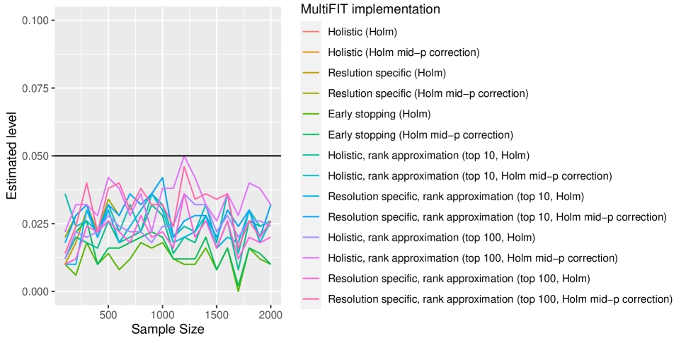
Figure S4: Estimated level versus sample size

The results confirm the theoretical guarantees that the level can be controlled at any given level $\alpha$. In fact, the procedure appears to be a bit conservative in controlling the level. Note, although $\mathbf{X}$ and $\mathbf{Y}$ are independent under the null hypothesis, the dependency structure between the different margins of $\mathbf{X}$ is arbitrary, as well as the dependency structure between the different margins of $\mathbf{Y}$. Therefore, this simulation is not exhaustive. However, we repeated the estimation of the level under various dependency structures for the margins, and the results are consistent with these that are shown here.

S5 Scaling: comparison of scenarios for MultiFIT

S6 Power study: sensitivity analysis for the parameters $p^{*}$ and $R^{*}$ of MultiFIT

In Figures S6 and S7 we demonstrate the effect of our main tuning parameters – $p^{*}$ and $R^{*}$ – on the estimated power. We evaluate the power for the simulation scenarios that are detailed in Table S1 over the grid $\mathbf{p}^{*}\times\mathbf{R}^{*}$ where $\mathbf{p}^{*}=\{0.005,0.01,0.05,0.1,0.5\}$ and $\mathbf{R}^{*}=\{1,2,3,4\}$. In general, higher $p^{*}$ and higher $R^{*}$ values entail more testing. Under some scenarios, where the dependency structure is “more local”, higher values are needed to ensure better power. When the dependency structures are “more global” we see that the selection of the tuning parameters makes little difference to the estimated power.

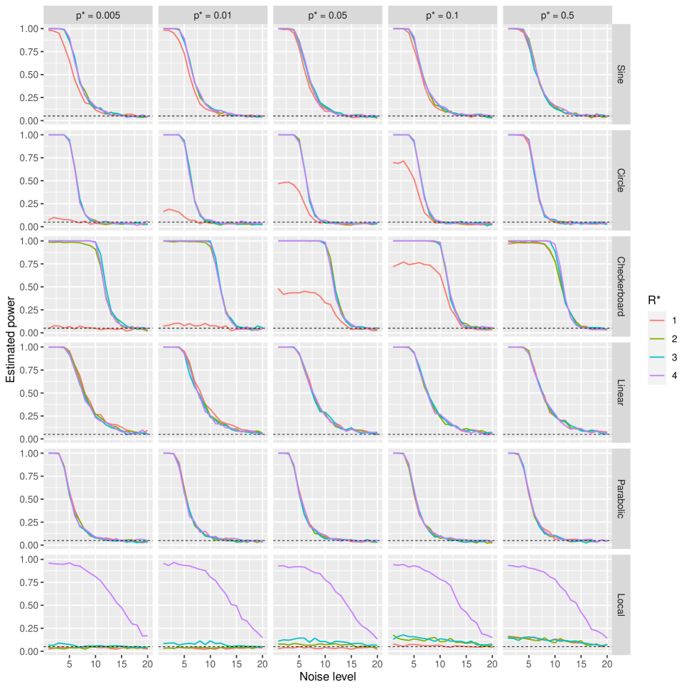
Figure S6: Power versus noise level for different methods. Estimated power at 20 noise levels for MultiFIT with different $p^{*}$ and $R^{*}$ values under the six scenarios from Table S1.

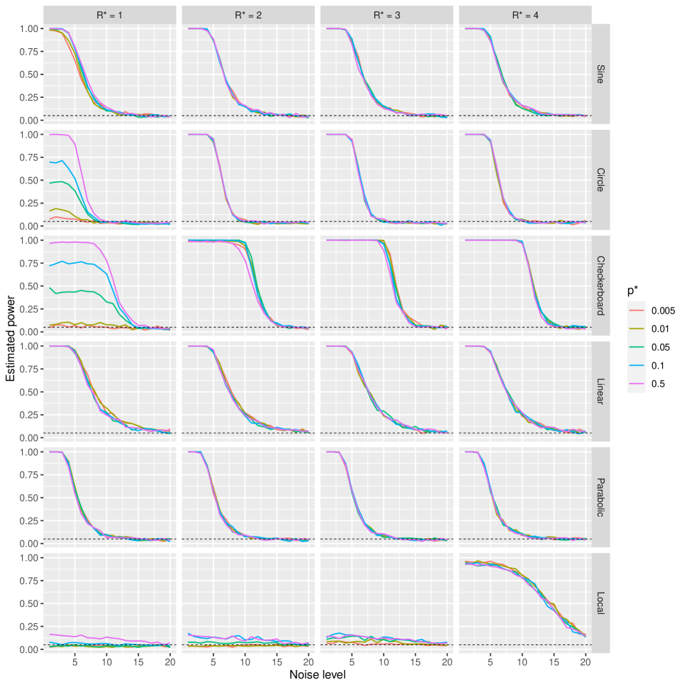
Figure S7: Power versus noise level for different methods. Estimated power at 20 noise levels for MultiFIT with different $p^{*}$ and $R^{*}$ values under the six scenarios from Table S1.

References

- Agresti and Gottard, (2007) Agresti, A. and Gottard, A. (2007). Nonconservative exact small-sample inference for discrete data. Computational Statistics & Data Analysis, 51(12):6447 – 6458.
- Bakirov et al., (2006) Bakirov, N. K., Rizzo, M. L., and Székely, G. J. (2006). A multivariate nonparametric test of independence. Journal of Multivariate Analysis, 97:1742–1756.
- Fan et al., (2017) Fan, Y., de Micheaux, P. L., Penev, S., and Salopek, D. (2017). Multivariate nonparametric test of independence. Journal of Multivariate Analysis, 153:189–210.
- Gretton et al., (2008) Gretton, A., Fukumizu, K., Teo, C. H., Song, L., Schölkopf, B., and Smola, A. J. (2008). A kernel statistical test of independence. In Platt, J. C., Koller, D., Singer, Y., and Roweis, S. T., editors, Advances in Neural Information Processing Systems 20, pages 585–592. Curran Associates, Inc.
- Heller et al., (2013) Heller, R., Heller, Y., and Gorfine, M. (2013). A consistent multivariate test of association based on ranks of distances. Biometrika, 100:503–510.
- Lee et al., (2019) Lee, D., Zhang, K., and Kosorok, M. R. (2019). Testing Independence with the Binary Expansion Randomized Ensemble Test. arXiv e-prints, page arXiv:1912.03662.
- Li and Yuan, (2019) Li, T. and Yuan, M. (2019). On the optimality of gaussian kernel based nonparametric tests against smooth alternatives.
- Ma and Mao, (2019) Ma, L. and Mao, J. (2019). Fisher exact scanning for dependency. Journal of the American Statistical Association, 114(525):245–258.
- Meintanis and Iliopoulos, (2008) Meintanis, S. G. and Iliopoulos, G. (2008). Fourier methods for testing multivariate independence. Computational Statistics & Data Analysis, 52:1884–1895.
- Pfister et al., (2018) Pfister, N., Bühlmann, P., Schölkopf, B., and Peters, J. (2018). Kernel-based tests for joint independence. Journal of the Royal Statistical Society: Series B (Statistical Methodology), 80(1):5–31.
- Székely and Rizzo, (2009) Székely, G. J. and Rizzo, M. L. (2009). Brownian distance covariance. The Annals of Applied Statistics, 3(4):1236–1265.
- Székely and Rizzo, (2013) Székely, G. J. and Rizzo, M. L. (2013). The distance correlation t-test of independence in high dimension. Journal of Multivariate Analysis, 117:193 – 213.
- Weihs et al., (2018) Weihs, L., Drton, M., and Meinshausen, N. (2018). Symmetric rank covariances: a generalized framework for nonparametric measures of dependence. Biometrika, 105(3):547–562.
- Zhang, (2019) Zhang, K. (2019). BET on independence. Journal of the American Statistical Association. Accepted.
- Zhou, (2019) Zhou, Q. (2019). Asymptotics of multivariate contingency tables with fixed marginals. Journal of Statistical Planning and Inference, 198:165–170.