On the decentralized navigation of multiple packages on transportation networks

Abstract

We investigate by numerical simulation and finite-size analysis the impact of long-range shortcuts on a spatially embedded transportation network. Our networks are built from two-dimensional ($d=2$) square lattices to be improved by the addition of long-range shortcuts added with probability $P(r_{ij})\sim r_{ij}^{-\alpha}$ [J. M. Kleinberg, Nature 406, 845 (2000)].Considering those improved networks, we performed numerical simulation of multiple discrete package navigation and found a limit for the amount of packages flowing through the network. Such limit is characterized by a critical probability of creating packages $p_{c}$, where above this value a transition to a congested state occurs. Moreover, $p_{c}$ is found to follow a power-law, $p_{c}\sim L^{-\gamma}$, where $L$ is the network size. Our results indicate the presence of an optimal value of $\alpha_{\rm min}\approx 1.7$, where the parameter $\gamma$ reaches its minimum value and the networks are more resilient to congestion for larger system sizes. Interestingly, this value is close to the analytically found value of $\alpha$ for the optimal navigation of single packages in spatially embedded networks, where $\alpha_{\rm opt}=d$. Finally, we show that the power spectrum for the number of packages navigating the network at a given time step $t$, which is related with the divergence of the expected delivery time, follows a universal Lorentzian function, regardless the topological details of the networks.

I Introduction

The navigation problem consists of sending a message, or some piece of information, from a given source node to a target node of a network ref:newman2010 ; ref:barthelemy2011 . Taking this perspective into account, communication networks, the internet, the network of streets for public transportation, all share the same basic purpose: to deliver the desired packages as faster as possible to their destiny, while maintaining its functionality. From this point of view, the 1967 small-world experiment proposed by the American psychologist Stanley Milgram is a paradigmatic example ref:milgram1967 . The algorithmic approach of the experiment performed later by Kleinberg ref:kleinberg2000 , not only had shown that a navigation guided solely by decentralized algorithms is capable of accomplish the task, but also that the underlying dimension of the spatially embedded network can drastically affect the expected delivery time. In the present work, we investigate the impact of the underlying geography of the transportation network on the navigation of multiple packages where a load limit to the network nodes exists.

In many transportation networks of interest in science and technology, efficient transport of information packages, energy, or even people is thought in terms of avoiding congestion rather than minimizing expected delivery time ref:arenas2001 ; ref:guimera2002a ; ref:guimera2002b . For instance, when using a crowdsourcing map application to navigate a city, the driver usually sacrifices time travel, adopting a longer detour in order to avoid traffic jams. Consider now that, by the addition of new shortcuts, we aim to plan or improve an existing transportation network. As we shall show, to consider the underlying structure of such network, while adding shortcuts, plays an important role in the way the transportation occurs, allowing the increase of the number of packages traveling the network, without missing its functionality.

The framework of spatially embedded networks makes use of a regular lattice of dimension $d$ with long-range connections randomly added upon it. Generally, it considers the addition of long-range connections between two given nodes $i$ and $j$ with a probability decaying with their lattice distance $r_{ij}$, $P(r_{ij})\sim r_{ij}^{-\alpha}$ ref:kleinberg2000 . The interplay between the underlying regular structure and a randomized long-range construction is a well-known recipe to mimic the so called small-world phenomenon ref:watts1998 , where the typical distance $\ell$ between a pair of nodes grows slowly with the number of nodes $N$ of the network, $\ell\sim{\rm log}N$ ref:barthelemy1999 . However, for the case of spatially embedded networks, this is true only for $\alpha\leq d$ ref:kosmidis2008 ; ref:chen2016 . Remarkably, the small-world property can be accessed by a decentralized algorithm only when $\alpha=d$ ref:kleinberg2000 ; ref:carmi2009 ; ref:cartozo2009 ; ref:hu2011a ; ref:hu2011b , a result that holds for fractals ref:roberson2006 ; ref:rozenfeld2010 , for transport phenomena that obeys local conservation laws (ref:oliveira2014, ; ref:sampaio2016, ), nonlocal percolation rules ref:reis2012 and brain networks ref:gallos2012a ; ref:gallos2012b . Moreover, when a cost constrain is imposed on the addition of shortcuts to the underlying network, it has been found that the better conditions to navigation are attained when $\alpha=d+1$ ref:gli2010 ; ref:yang2010 ; ref:yli2010 ; ref:gli2013 . It is argued that such conditions, with and without cost constrain, are optimal due to strong correlations between the underlying spatial network and the long-range structure, allowing the package holder to find the shortest paths at the small-world network ref:kleinberg2000 . It is claimed that such compromise between local and long-range structures leads to an effective dimension higher than the dimension of the underlying local structure ref:daqing2011 ; ref:boguna2009 .

The remaining of this manuscript is organized as follows. In Section II we describe the spatially embedded network model proposed by Kleinberg ref:kleinberg2000 . The rules for node overload used in the present study in order to mimic the onset of congestion are also presented in Sec. II. In Section III the results of our simulations and numerical analysis are presented, where we study the behavior of the order parameter, the scale of the critical point and the divergence of the characteristic time. We leave further discussion and conclusions to Section IV.

II Model formulation

Using a simple and general model based on a decentralized algorithm, we study the effects of nonlocality assuming three simple ingredients ref:arenas2001 ; ref:guimera2002b . The first is a physical spatially embedded structure where the transportation process takes place, in other words, the transport network itself. Second, we assume that the channels through which the information flows have limited capacity. Finally, the information navigating this network is composed of discrete packages. Without lack of generality, the important characteristics of the problem are obtained by the analysis of the navigation and congestion of these discrete packages.

As shown in Fig. 1, the transportation network is embedded in a square lattice with $N=L\times L$ nodes upon which we add long-range connections. In this model, pairs of nodes $i$ and $j$ are chosen at random to receive one of those long-range connections with probability proportional to $r_{ij}^{-\alpha}$, where $r_{ij}$ is the Manhattan distance between nodes $i$ and $j$. Since the number of nodes separeted by the lattice distance $r$ from a node $i$ in a $d$-dimensional lattice is proportional to $r^{d-1}$ (see Fig. 1), the probability $P(r_{ij})$ can be mapped into the density distribution function $p(r)\sim r^{d-1-\alpha}$. After the distance $r$ is chosen following the distribution $p(r)$, we randomly choose node $j$ from the set of nodes separated from $i$ by the distance $r$. Clearly, the present model satisfies the small-world paradigm, i.e., it is rich in short-range connections, but has only a few long-range connections (ref:watts1998, ).

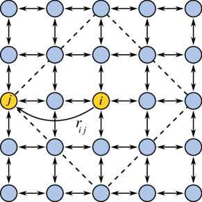
Figure 1: Kleinberg networks are built by adding long-range connections on regular lattices. For a given node $i$, a node $j$ is randomly chosen and an undirected link of length $r_{ij}$ is added between them with probability $P(r_{ij})\sim r_{ij}^{-\alpha}$. By doing so, the node $j$ can be any node with a Manhattan distance of $r_{ij}$. The dashed lines highlight the eight nodes separated from node $i$ by a lattice distance $r=2$. We randomly choose the node $j$ from this set of eight nodes.

The package transportation algorithm is defined as follows. At first, we assign to the whole network a probability $p$ for the creation of information packages. After that, at each time step $t$, we draw a uniformly distributed random number in the interval ranging from 0 to 1 for each node $s$. If this number is smaller than $p$, a package of information is created at node $s$. Then, for each new package a target node $t$ is randomly assigned. In other to mimic real life situations, the nodes (e.g., the routers from the Internet) do not have information about the whole network topology. Therefore, an information holder node $a$ chooses from its set of neighbors, both short- and long-range, the neighbor node $b$ that is geographically closer to $t$ to send the package. Clearly, this algorithm has close relationship with the greedy algorithm proposed by Kleinberg utilized to study the problem of efficient navigation of one package of information in small-world networks (ref:kleinberg2000, ).

After the next potential holder is chosen, the package is transmitted or not from node $a$ to node $b$ through a channel (link) of quality $q_{ab}$ ref:arenas2001 . In real life situations, such quality influences the transmission probability, and it is expected to depend on the package load of the nodes it connects. Accordingly, the capacity $\kappa_{a}$ of node $a$ to receive a new package can be defined as

$$\kappa_{a}=\left\{\begin{array}[]{ll}1,&{\rm if~{}}n_{a}=0;\\ n_{a}^{-\xi},&{\rm if~{}}n_{a}=1,2,3,...;\end{array}\right.$$ (1)

where $n_{a}$ is the number of packages at node $a$. Thus, one can define the channel quality as the geometric average $q_{ab}=\sqrt{\kappa_{a}\kappa_{b}}$ (ref:arenas2001, ). Then, we can rewrite channel quality as

$$q_{ab}=(n_{a}n_{b})^{-\xi/2}.$$ (2)

Assuming $q_{ab}$ as the probability of node $a$ to deliver a package to node $b$, the average number $\langle n_{ab}\rangle$ of packages delivered from $a$ to $b$ per time unit will be proportional to $n_{a}^{1-\xi/2}n_{b}^{-\xi/2}$ (ref:arenas2001, ). Note that the packages are uniformily created across the network, therefore, we can assume $n_{a}\sim n_{b}$. Consequently,

$$\langle n_{ab}\rangle\sim n_{a}^{1-\xi}.$$ (3)

When $\xi<1$, the average number of delivered packages increases with the package load of nodes, and for this reason, the system is always found at a free-flow phase. On the other hand, if $\xi>1$, the average number of delivered packages decays fast, meaning that nodes fail to deliver the packages, causing the emergence of a congested phase. Along these lines, the present model has a clear phase transition from a free-flow phase to a congested one at $\xi=1$. In what follows, we focus our study at this critical value of $\xi$.

III Results and Discussion

III.1 Transition from free phases to congested phases

According to the previous discussion, for $\xi=1$, we expect to have both free flow and congestion phases depending of the probability $p$. Therefore, we start our analysis by defining and computing the order parameter $\eta$ given by

$$\eta(p)=\lim_{t\rightarrow\infty}\frac{1}{pL^{2}}\frac{\langle\Delta N\rangle}{\Delta t},$$ (4)

where $pL^{2}$ is the average number of packages created per time step, $\Delta N$ is the number of undelivered packages navigating the network at time windows of duration $\Delta t$. At stationary states ($t\rightarrow\infty$), the average $\langle\Delta N\rangle$ is related with the rate of creating packages and the rate of delivering packages per time step, and therefore, it depends only on $p$ at large $t$, since $\Delta N$ will be proportional to the duration of the time windows $\Delta t$ (ref:arenas2001, ; ref:guimera2002b, ).

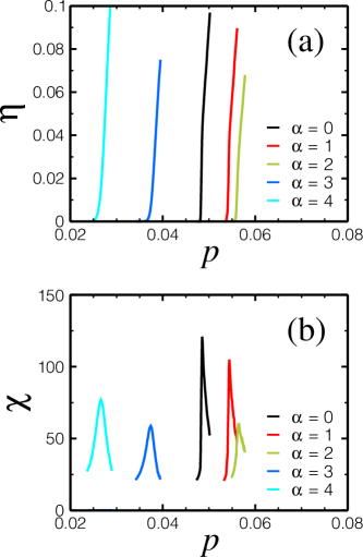
Figure 2: Transition to congested phases for different values of $\alpha$. In (a) we show the order parameter $\eta$ as a function of the probability of creating new packages $p$. When the network topology favors the decentralized delivery algorithm, the packages are delivered in a high rate than new packages are created, avoiding nodes to become overloaded, therefore preventing congestion. This is the case of $\alpha=0$, $1$, and $2$, where the transition occurs for higher values of $p$. As depicted in (b), the critical threshold $p_{c}$ marks a maximum value on the response susceptibility $\chi$. Here, we use $L=128$ with $T=10^{4}$ for each value of $\alpha$ and simulation time equal to $10^{5}$.

As depicted in Fig. 2(a), the analysis of the order parameter $\eta$ allows us to define the critical probability of creating new packages $p_{c}$, characterizing a typical second-order phase transition between congested and free phases (ref:arenas2001, ; ref:guimera2002a, ; ref:guimera2002b, ). For small values of $p$, $\langle\Delta N\rangle=0$ at the stationary state, resulting on free phases, meaning that the rate of creating packages is smaller than the rate of delivering packages. As $p$ increases, the rate of creating packages also increases, till it reaches the critical threshold $p_{c}$, where the rate of created packages is equal to the supported rate of delivering packages. Beyond this critical threshold, the value of $\langle\Delta N\rangle$ increases with $t$, resulting on values for $\eta>0$, marking the existence of a congested phase.

Interestingly, $p_{c}$ presents a nontrivial behavior with $\alpha$ on Kleinberg networks, as depicted in Fig. 2(a). Specifically, when $\alpha>0$, the critical threshold slightly increases ($\alpha=1$ and $2$), showing that at this range of $\alpha$ the networks are more resilient to the creation of information packages. However, for larger values of the exponent $\alpha$, $\alpha=3$ and $4$, the critical threshold drastically decreases leading to networks more prone to congestion.

III.2 Behavior of the critical threshold

Next, we investigate the behavior of $p_{c}$. Second-order phase transitions are expected to be dominated by larger fluctuations on the order parameter close to their critical threshold (ref:stanley1971, ). Thus, in order to compute $p_{c}$ with precision, it is convenient to define a macroscopic susceptibility function $\chi(p)$ as

$$\chi(p)=\lim_{T\rightarrow\infty}T\sigma_{\eta}(T),$$ (5)

where $\sigma_{\eta}(T)$ is the standard deviation of the order parameter computed in many time windows of width $T$. Hence, in order to compute $\chi(p)$, it is necessary quite a long simulation time for one single realization. In the context of critical phenomena, such function is sensitive to fluctuations of the order parameter, where it diverges as the control parameter approaches its critical value ref:stanley1971 . As shown in Fig. 2(b), $\chi(p)$ presents a maximum at nontrivial values of $p$ for different value of $\alpha$. Accordingly, we identify these values as $p_{c}$ (ref:arenas2001, ; ref:guimera2002b, ).

Figure 3: Behavior of the critical point $p_{c}$. In panel (a) we show the critical probability $p_{c}$ as a function of the exponent $\alpha$. As the system size $L$ increases, the packages take longer to be delivered, causing the increase of $\Delta N$. As a consequence of that, the transition to congested phases occurs for even smaller values of $p_{c}$. However, independently of the value of $L$, the critical probability always presents a maximum as $\alpha$ approaches the value of $\alpha=2$. The critical probabilities follow a power-law behavior, $p_{c}\sim L^{-\gamma}$, as presented in the main plot of (b). The values of the exponent $\gamma$ resulting from a least-square fitting to the data are presented in the inset, where a non-monotonic behavior can be clearly observed. Here, we use $L=2^{5}$ with $T=10^{4}$ for each value of $\alpha$ and simulation time equal to $10^{5}$.

In order to determine how the exponent $\alpha$ affects the network’s resilience to congestion, we study the dependence of the critical point $p_{c}$ with the linear size $L$ for different values of $\alpha$. Figure 3(a) shows the estimated values of $p_{c}$ as a function of the exponent $\alpha$ for three different system sizes. In accordance with the results for $\eta(p)$ and $\chi(p)$, the critical point $p_{c}$ presents similar behavior with respect to $\alpha$. As presented in Fig. 2, $p_{c}$ increases with $\alpha$ for $0<\alpha<2$. However, it decreases for $2<\alpha<4$, and finally saturates and reaches its lower values for $\alpha>4$.

The way in which $p_{c}$ scales with $L$, however, follows rather different behaviors, depending of the values of $\alpha$. As presented in the main plot of Fig. 3(b), our results suggest that the critical point $p_{c}$ follows a scaling law with size $L$ following a power-law function, $p_{c}\sim L^{-\gamma}$. This power-law behavior provides an important piece of information about our model: as the system size increases, and consequently the distance between source nodes and target nodes also increases in average, more packages are navigating the network at a given time step. This makes larger networks more susceptible to congestion, since the expected number of packages occupying a node increases. For the case of mobility patterns in cities, this result agrees with the allometric relations between the city population and the total traffic delay ref:louf2014 and traffic accidents ref:melo2014 . Moreover, the different values of the scaling exponent $\gamma$ suggest that for a given system size $L$, there are values of $\alpha$ that generate networks more robust to package transportation.

We extract more information about this scaling by performing extensive simulations for different values of $\alpha$ and very long realizations for different system sizes. In each case, the critical point $p_{c}$ is estimated by the computation of the susceptibility $\chi(p)$. The inset in Fig. 3(b) shows the values of the exponent $\gamma$ as a function of exponent $\alpha$. As one can see, as $\alpha$ increases, $\gamma$ slightly decreases from $\gamma=0.6(9)$ at $\alpha=0$, to close to $\gamma=0.6(1)$, when $\alpha$ approaches the dimension of the underlying network, $\alpha=2$. Here, we obtain the minimum value of $\gamma$ for $\alpha_{\rm min}=1.7$, where $\gamma=0.6(0)$. For $2<\alpha<4$, the value of the exponent $\gamma$ sharply increases. For the range of $4<\alpha<10$, the values of $\gamma$ increases very slowly. We found the values of $\gamma=0.9(3)$ for $\alpha=4$, and $\gamma=1.0(3)$ for $\alpha=10$.

The nonmonotomic behavior of $\gamma$ can be better understood by the analysis of the single-package navigation case. For this case, under decentralized algorithms, similar behavior was found in the same topology for the scaling of the expected delivery time ref:kleinberg2000 ; ref:rozenfeld2010 ; ref:carmi2009 ; ref:cartozo2009 . Precisely, the value of the exponent $\alpha$ that optimizes the delivery time of a package in two dimensions is $\alpha_{\rm opt}=2$, where the expected delivery time scales logarithmic with $L$. For $\alpha$ different from the underlying network dimension $d$, the expected delivery time has a power-law behavior, $L^{x}$ ref:carmi2009 ; ref:cartozo2009 . In this situation, the value $\alpha=d$ is a transient point for which, $x=(d-\alpha)/(d+1-\alpha)$ for which $\alpha<d$, and $x=\alpha-d$ for $\alpha>d$. We believe that the different value found for the minimum, $\alpha_{\rm min}=1.7$, results from the small network sizes used due to the long simulation time necessary for the computation of $\chi(p)$. Hence, we conjecture that this optimal value, $\alpha_{\rm opt}=2$, would help in postponing the emergence of congestion for the case of multiple package navigation.

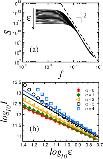
Figure 4: (a) Power spectrum of $S$ as a function of $f$ for $\alpha=0$, and for the free phase, $p<p_{c}$. As one can see, for all values of the rescaled control parameter $\varepsilon$, $S$ has the form of a Lorentzian function given by Eq. (6). The values of $\varepsilon$ increase from the top to the bottom. Therefore, the curves at the top are closer to the critical value $p_{c}$. Provided the Lorentzian behavior, it is expected a power-law decay of $S$ for larger values of $f$, as shown by the dashed line with slope $-2$. (b) Intensity $I$ as a function of the order parameter $\varepsilon$ obtained from the non-linear curve fitting of $S$ using Eq. (6), for different values of $\alpha$ at the free phase. The plot suggests that $I\sim\varepsilon^{-\zeta}$. For $\alpha=3$ and $4$, the estimated values of $I$ deviates from this behavior when the system approaches the transition at the lower values of $\varepsilon$. The solid lines are the fitting results using $I\sim\varepsilon^{-\zeta}$ at the ranges of $\varepsilon$ where such power-law behavior holds. Each power spectrum is obtained through an average of 100 realizations, with $L=32$ and simulation time equal to $10^{5}$.

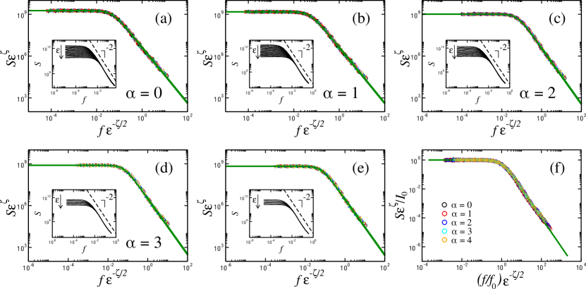
Figure 5: Data collapse of the power spectrum $S$ for different values of the control parameter $\varepsilon$ and (a) $\alpha=0$, (b) $\alpha=1$, (c) $\alpha=2$, (d) $\alpha=3$, and (e) $\alpha=4$. We use $\zeta=2.2(0)$, $2.3(3)$, $2.6(0)$, $2.9(1)$, and $3.0(9)$ for $\alpha=0$, $1$, $2$, $3$, and $4$, respectively. These values were obtained from a least-square fitting to the data presented at Fig. 4(b). The inset in each plot is the original data for the power spectrum $S$ obtained from our simulations. (f) When the plot axes are scaled using $S\varepsilon^{\zeta}/I_{\rm 0}$ and $\left(f/f_{\rm 0}\right)\varepsilon^{-\zeta/2}$, all data presented at the panels (a)-(e) collapse into the universal Lorentzian function $\mathcal{L}$. Each power spectrum is obtained through an average of 100 realizations, with $L=32$ and simulation time equal to $10^{5}$.

III.3 Divergence of expected delivery time

Now, we focus our attention on the divergence of the expected delivery time. To do this, we analyze the behavior of the power spectrum of $N(t)$ defined as the Fourier transform $S(f)=\mathcal{F}\{N(t)\}$, where $f$ is the frequency associated with package delivery. In Fig. 4(a), we show $S$ as a function of $f$ for different values of the rescaled control parameter $\varepsilon=|p-p_{c}|/p_{c}$ at the free phase, $p<p_{c}$, with $\alpha=0$. As depicted, the power spectrum $S$ has the form of a Lorentzian function given by:

$$S=\frac{I}{1+\left(\frac{f}{f_{\rm c}}\right)^{2}},$$ (6)

where the intensity $I$ is the maximum value of $S$, and $f_{\rm c}$ is a characteristic frequency. The intensity parameter $I$ is associated with the the width of the Lorentzian function. On the other hand, the characteristic frequency $f_{\rm c}$ is closely related with the average time of delivering a package $\tau\sim 1/f_{\rm c}$. As one can see in Fig. 4(a), as $\varepsilon$ decreases, the width of the plateau marking the value of $I$ also decreases, and at the limit $\varepsilon\rightarrow 0$ the power spectrum must scales as $1/f^{2}$. This is a signature of the divergence of the average expected delivery time, leading to $f_{\rm c}\rightarrow 0$ as $\varepsilon\rightarrow 0$, since $\tau\sim\varepsilon^{-z}$ ref:guimera2002a .

To better analyze the divergence of $\tau$ close to the transition, we compute the values of the exponent $z$ through the analysis of $I$ as a function of $\varepsilon$. As $\varepsilon\rightarrow 0$, it is expected that $I\sim\varepsilon^{-\zeta}$. Moreover, the exponent $z$, describing the divergence of the expected delivery time, must be related with $\zeta$ by the equation $z=\zeta/2$ ref:guimera2002a . In Fig. 4(b), we show the values of $I$, collected from the nonlinear curve fitting of $S$ using Eq. 6, as a function of $\varepsilon$ in a log-log fashion. For $\alpha=0$, $1$, and $2$, we found $\zeta=2.2(0)$, $2.3(3)$, and $2.6(0)$, respectively. For $\alpha=3$ and $4$, the behavior of $I$ differs from such scaling as $\varepsilon\rightarrow 0$. Due to the Lorentzian profile, as $p$ approaches its critical value $p_{c}$, the width of the Lorentzian function diminishes, since $S\sim 1/f^{2}$ at this limit, resulting on an overestimation of $I$. Thus, in order to estimate $\zeta$, we use the range of $\varepsilon$ where the power-law behavior of $I$ holds. By doing this, we found $\zeta=2.9(1)$ and $3.0(9)$ for $\alpha=3$ and $4$, respectively. Therefore, since $\tau\sim\varepsilon^{-\zeta/2}$, the monotonic increase of $\zeta$ with $\alpha$ leads to the conclusion that $\tau$ diverges faster for higher values of $\alpha$ as the system approaches the transition point. The results for $\zeta$ and the resilience to congestion with system size (see Fig. 3) leads to a better compromise for transportation conditions attained when $\alpha\approx 2$. Therefore, based on previous results reported in the literature ref:kleinberg2000 ; ref:kosmidis2008 ; ref:carmi2009 ; ref:cartozo2009 ; ref:roberson2006 ; ref:oliveira2014 ; ref:gli2010 ; ref:yang2010 ; ref:yli2010 ; ref:gli2013 , we conjecture that the optimal condition to the navigation of multiple packages on spatially embedded networks is obtained when $\alpha=d$, where $d$ is the dimension of the underlying network.

Interestingly, the scaling relations $I=I_{\rm 0}\varepsilon^{-\zeta}$ and $f_{\rm c}=f_{\rm 0}\varepsilon^{\zeta/2}$ allow us to write Eq. 6 in the more general form

$$S^{\prime}=\varepsilon^{-\zeta}S(f\varepsilon^{\zeta/2}).$$ (7)

As depicted in Figs. 5(a)-(e), all data for $S\varepsilon^{\zeta}$ as a function of $f\varepsilon^{-\zeta/2}$ collapse into a unique behavior for all values of $\alpha$. If one uses the values obtained for $I_{\rm 0}$ and $f_{\rm 0}$ (see Fig. 5(f)), the rescaling of the plot axes shows that, regardless of the topological details of the network defined by $\alpha$, all simulation data collapse into a universal curve described by the Lorentzian

$$\mathcal{L}=\frac{1}{1+F^{2}},$$ (8)

where $F=(f/f_{\rm 0})\varepsilon^{-\zeta/2}$ and $\mathcal{L}=S^{\prime}/I_{\rm 0}$. Since the addition of shortcuts change the effective dimension of the network ref:daqing2011 , we believe that this Lorentzian behavior must hold for any network topology, such as the one-dimensional and two-dimensional lattices, as well as the Cayley tree ref:guimera2002a .

IV Conclusions

In order to reveal the role of network topology on the transport of information packages, we studied the dynamics of a simple and general model of transportation networks on spatially embedded networks. By assuming additional long-range connections added to a two dimensional square lattice following a power-law distribution $P(r_{ij})\sim r_{ij}^{-\alpha}$, we found a limit for the total amount of information packages flowing through the network characterized by a critical probability of creating new packages $p_{c}$. Our results show that $p_{c}$ is described by a power-law of the network linear size, $p_{c}\sim L^{-\gamma}$, as it has been found in other topologies ref:guimera2002b . Remarkably, due to the characteristics of the network model used, $\gamma$ presents a nontrivial dependence with the topological parameter $\alpha$. Specifically, $\gamma$ has a minimum for $\alpha_{\rm min}=1.7$, meaning that, in this case, the network is more resilient to the creation of new information packages. Since the transportation algorithm makes use only of local knowledge of the network geography, this robustness condition coincides with the small-world regime of the network ref:kosmidis2008 . Moreover, it is close to the optimal navigation condition for a single package on two dimensions, $\alpha_{\rm opt}=2$. Therefore, the spatial peculiarities of the network play a major role on the robustness of multiple package transportation. In other words, when optimizing the resilience of information exchange on transportation networks, one should take into account not only the protocol adopted, but also look for hints provided by the analysis of its geographical properties. These results leads us to conjecture that the optimal navigation of multiple packages in spatially embedded networks is attained when $\alpha_{\rm opt}=d$, in the same way as in the optimal navigation of single packages ref:kleinberg2000 ; ref:kosmidis2008 ; ref:carmi2009 ; ref:cartozo2009 ; ref:roberson2006 ; ref:oliveira2014 ; ref:gli2010 ; ref:yang2010 ; ref:yli2010 ; ref:gli2013 .

In addition, beyond the robustness of transportation networks, we studied its critical behavior by analyzing the power spectrum of the total number of packages as a function of time. When $p<p_{c}$, these spectra are described by a Lorentzian function, and saturate at a characteristic value $I$. In contrast, when $p$ approaches $p_{c}$, the power spectra present a power-law behavior with exponent $-2$. Considering the characteristic saturation value $I$ and its power-law behavior described by the exponent $\zeta$, we were able to show that the power spectra collapse into a universal Lorentzian function, regardless the topological details of the networks and their embedding dimension. These power spectra provide the divergence of relevant quantities for practical purposes, as the average time of delivering a package and the number of packages navigating the network. We expect that the modeling approach and results presented here could be useful in further studies on the multiple package navigation problem in different network topologies, which might lead to significant improvements on the ever-present package delivering processes occurring in real transportation networks.

References

- (1) M. E. J. Newman, Networks: An Introduction (Oxford University Press, 2010).
- (2) M. Barthélémy, Phys. Rep. 499, 1 (2011).
- (3) S. Milgram, Psycology Today 2, 60 (1967).
- (4) J. M. Kleinberg, Nature 406, 845 (2000).
- (5) H. E. Stanley, Introduction to Phase Transitions and Critical Phenomena (Oxford University Press, 1971).
- (6) A. Arenas, A. Díaz-Guilera, and R. Guimerà, Phys. Rev. Lett. 86, 3196 (2001).
- (7) R. Guimerà, A. Arenas, A. Díaz-Guilera, and F. Giralt, Phys. Rev. E 66, 026704 (2002).
- (8) R. Guimerà, A. Díaz-Guilera, F. Vega-Redondo, A. Cabrales, and A. Arenas, Phys. Rev. Lett. 89, 248701 (2002).
- (9) D. J. Watts and S. H. Strogatz, Nature 393, 440 (1998).
- (10) M. Barthélémy and L. A. N. Amaral, Phys. Rev. Lett. 82, 3180 (1999).
- (11) K. Kosmidis, S. Havlin, and A. Bunde, Europhys. Lett. 82, 48005 (2008).
- (12) Q. Chen, J.-H. QIan, L. Zhu, and D.-D. Han, Phys. Rev. E 93 032321 (2016).
- (13) S. Carmi, S. Carter, J. Sun, and D. ben-Avraham, Phys. Rev. Lett. 102, 238702 (2009).
- (14) C. C. Cartozo and P. De Los Rios, Phys. Rev. Lett. 102, 238703 (2009).
- (15) Y. Hu, Y. Wang, D. Li, S. Havlin, and Z. Di, Phys. Rev. Lett. 106, 108701 (2010).
- (16) Y. Hu, J. Zhang, D. Huan, and Z. Di, Europhys. Lett. 96, 58006 (2011).
- (17) M. R. Roberson and D. ben-Avraham, Phys. Rev. E 74, 017101 (2006).
- (18) H. D. Rozenfeld, C. Song, and H. A. Makse, Phys. Rev. Lett. 104, 025701 (2010).
- (19) C. L. N. Oliveira, P. A. Morais, A. A. Moreira, and J. S. Andrade, Phys. Rev. Lett. 112, 148701 (2014).
- (20) C. I. N. Sampaio Filho, T. B. dos Santos, A. A. Moreira, F. G. B. Moreira, and J. S. Andrade, Phys. Rev. E 93, 052101 (2016).
- (21) S. D. S. Reis, A. A. Moreira, and J. S. Andrade, Phys. Rev. E 85, 041112 (2012).
- (22) L. K. Gallos, H. A. Makse, and M. Sigman, Proc. Natl. Acad. Sci. USA 109, 2825 (2012).
- (23) L. K. Gallos, M. Sigman, and H. A. Makse, Front. Physio. 3, 123 (2012).
- (24) G. Li, S. D. S. Reis, A. A. Moreira, S. Havlin, H. E. Stanley, and J. S. Andrade, Phys. Rev. Lett. 104, 018701 (2010).
- (25) H. Yang, Y. Nie, A. Zeng, Y. Fan, Y. Hu, and Z. Di, Europhys. Lett. 89, 58002 (2010).
- (26) Y. Li, D. Zhou, Y. Hu, and Z. Di, Europhys. Lett. 92, 58002 (2010).
- (27) G. Li, S. D. S. Reis, A. A. Moreira, S. Havlin, H. E. Stanley, and J. S. Andrade, Phys. Rev. E 87, 042810 (2013).
- (28) L. Daqing, K. Kosmidis, A. Bunde, and S. Havlin, Nat. Phys. 7, 481 (2011).
- (29) M. Boguna, D. Krioukov, and K. C. Claffy, Nat. Phys. 5, 74 (2009).
- (30) R. Louf and M. Barthélémy, Sci. Rep. 4, 5561 (2014).
- (31) H. P. M. Melo, A. A. Moreira, E. Batista, H. A. Makse, and J. S. Andrade, Sci. Rep. 4, 6239 (2014).