Circuit-based modular implementation of quantum ghost imaging

Abstract

Efforts on enhancing the ghost imaging speed and quality are intensified when the debate around the nature of ghost imaging (quantum vs. classical) is suspended for a while. Accordingly, most of the studies these years in the field fall into the improvement regarding these two targets by utilizing the different imaging mediums. Nevertheless, back to the raging debate occurred but with different focus, to overcome the inherent difficulties in the classical imaging domain, if we are able to utilize the superiority that quantum information science offers us, the ghost imaging experiment may be implemented more practically. In this study, a quantum circuit implementation of ghost imaging experiment is proposed, where the speckle patterns and phase mask are encoded by utilizing the quantum representation of images. To do this, we formulated several quantum models, i.e. quantum accumulator, quantum multiplier, and quantum divider. We believe this study will provide a new impetus to explore the implementation of ghost imaging using quantum computing resources.

1 Introduction

Leveraging on its immense potentials for applications that require minimal computing resources, speed, security, etc., quantum information science has exploded beyond its utility in optics (including laser technology [1] and remote sensing technology [2]) to exciting applications in computer science and engineering (e.g., machine learning [3] and artificial intelligence [4]). Naturally, this has also led to inter-disciplinary explorations, such as quantum ghost imaging [5] and quantum image processing [6], etc.

Ghost imaging is a technique employed to retrieve an object from the cross-correlation function of two separate beams and neither of which obtains the information from the object [7]. One beam interrogates a target and then illuminates a single-pixel detector that provides no spatial resolution, while the other beam does not interact with the target, but it impinges on a high-resolution camera, hence affording a multiple-pixel output [8]. The timeline for this sub-discipline’s development shows its modest beginning started in 1995, where the two beams of ghost imaging were formed from a stream of entangled photons [9]. The reconstruction of the image was attributed to the non-local quantum correlations between the photon pairs. For several years, the ghost imaging was considered as an effect of quantum non-locality due to the earlier experiments. Challenging this interpretation, Bennink et al. demonstrated ghost imaging using two classically correlated beams [10], following which, it was found that many of the features obtained with entangled photons could be reproduced with a classical pseudothermal light source. However, the nature of the spatial correlations exhibited with a pseudothermal source, and whether they can be interpreted as classical intensity correlations or are fundamentally non-local quantum correlations, is still under debate [11, 12, 13, 14]. Although, focusing on the problems and improvement of the spatial resolution, field of view, and signal-to-noise ratio of the ghost imaging result, researchers have gained a lot of progresses by using different types of light sources [15] and the implementations on different materials [16].

Even though the ghost imaging technique has shown potential for applications demanding high detection sensitivity as well as high resolution, which are useful in the civil and military domains, the following reasons impede its development to a large extent:

• To assure the quality of the ghost imaging result, a large amount of samplings for speckle patterns are required. Establishment (i.e. representation) and storage of these patterns will be a heavy job for classical computers.

• In order to generate the interested image, the interactions between the speckle patterns and the phase mask require a huge number of judgement (i.e. judging whether the pixel in the speckle patterns is in the subregion of the phase mask) which will cost a massive computing resources.

• Cross correlation of the signals in the signal and idler fields will also undertake a great deal of computations which is also a great trials to the classical computing devices.

Fortunately, these problems occurred on classical computing domain may be solved by utilizing the quantum computing framework [17, 18, 19]. Among many other areas, these tools are used in the emerging sub-discipline of quantum image processing. Technically, quantum image processing is focused on extending conventional image processing tasks and operations to the quantum computing framework [20, 21, 22]. It is primarily devoted to utilizing quantum computing technologies to capture, manipulate, and recover quantum images in different format and for different purposes [23]. Due to some astounding properties of quantum computation (i.e. entanglement and parallelism), it is anticipated that quantum image processing will offer incredible capabilities and performances in terms of computing speed, guaranteed security, and minimal storage requirements, etc. [23]. The pioneering work of quantum image processing should be attributed to Venegas-Andraca and Bose’s Qubit Lattice [24] description for quantum images in 2003, while the proposal of flexible representation for quantum images [25] by Le et al. in 2010 receives more attention since it supports the integration of the quantum image into a normalized state and facilitates auxiliary transformations on the content of the image. Following these, many other quantum image representations have been proposed [26, 27] as well as an array of algorithmic frameworks that target the spatial or chromatic content of the image [28, 29, 30, 31].

In this study, we attempt to utilize the proven potency of quantum information processing, i.e. quantum image processing, in a new paradigm for ghost imaging. The advantages are provided as follows:

• Quantum register which includes n quits is able to store $2^{n}$ binary numbers. Such exponential storage ability (in comparison with the classical register/storage) on quantum computers could solve the problem that large amounts of speckle patterns occupy too much storage space commendably.

• The judgements required in the interaction between the speckle patterns and the phase mask could be simply done by several quantum CNOT gates. Utilizing the parallelism of quantum computing, the complexity of the whole simulating calculation would be greatly reduced.

• Cross correlation at the final step would also benefit from the parallelism of quantum computing. By designing the quantum arithmetic operations, i.e. quantum accumulator, quantum multiplier, and quantum divider, the efficient operations (and circuit implementation) of the cross correlations could be assured.

The rest of the paper is organized as follows: in Section 2, quantum image representation, quantum adder, and quantum comparator are introduced, following these, the quantum accumulator, quantum multiplier, and quantum divider are designed and proposed. In Section 3, a complete quantum ghost imaging circuit is established including the creation of quantum speckle patterns, the interaction between the patterns and the quantum phase mask, and quantum computation of the cross-correlation. The conclusions of the study and its applications on the quantum image encryption are discussed in Section 4.

2 Modular approach to basic quantum arithmetic operations

Traditionally, the arithmetic operation of addition, subtraction, multiplication, and division are employed to operation on two or more numbers. As quantum states, it is infeasible to extend classical execution of these operations as natural numbers to our quantum ghost imaging (QGI) framework. In addition to the four traditional operations, we utilize the accumulator (ACC) and comparator (COM) operations as the quantum arithmetic operations to support the execution of our proposed QGI protocol. First, we formalize, from established literature, the notion of an image as used on the quantum computing paradigm.

2.1 Quantum image representation

As defined in [20], quantum image processing is devoted to “utilizing the quantum computing technologies to capture, manipulate, and recover quantum images in different formats and for different purposes.” The first step accomplishing this requires representation to encode images based on the quantum mechanical composition of any potential quantum computing hardware be conjured [32]. Among all of the available quantum image representations, in this study, the novel enhanced quantum representation of digital images [33] is utilized to represent the speckle pattern and the target image, which supports the use of the basis states of two qubit sequence to store the chromatic and spatial content each pixel in the image and mathematically defined as follows:

$$|I(m,n,p)\rangle ={1\over 2^{(m+n)/2}}\sum_{y=0}^{2^{m}-1}\sum_{x=0}^{2^{n}-1}\bigotimes_{h=0}^{l-1}|c_{yx}^{h}\rangle|yx\rangle,$$ (1)

where $|c_{yx}^{h}\rangle$ ($c_{yx}^{h}\in\{0,1\}$) encodes the chromatic information of the pixel at position $|yx\rangle$, where $|yx\rangle=|y\rangle|x\rangle=|y_{m-1}y_{m-2}\ldots y_{0}\rangle|x_{n-1}x_{n-2}\ldots x_{0}\rangle$. An example of a $2\times 2$ quantum image and its quantum state is presented in [23], wherein, its preparation and retrieval procedures have been thoroughly discussed.

2.2 Quantum adder

Quantum adder (hereinafter called ADD module) is considered a basic quantum arithmetic operation in the quantum computing field [34]. The aim of ADD module is to perform the following equation:

$$\text{ADD}|y,x\rangle=|y,y+x\rangle,$$ (2)

where $|y\rangle$ and $|x\rangle$ are two input quantum kets and the two output kets are $|y\rangle$ and $|y+x\rangle$. As presented in Figure 1, a quantum adder consists of $2n-1$ carry modules and $2n$ sum modules. In addition, the carry module could be decomposed to 2 Toffoli gates and 1 CNOT gate, while the sum module could be executed by 2 CNOT gates as presented in Figure 1(a) and (b). Moreover, as discussed in [34] and [35], quantum subtraction could be implemented using a network of quantum adder(s) due to the fact that quantum gates are reversible. To illustrate the subtracter (i.e. SUB), a black bar is inserted on the left side of the module block.

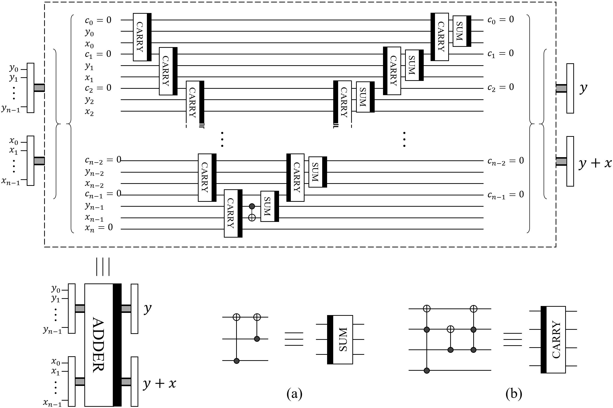
Figure 1: Circuit implementation of quantum ADD module (figure and descriptions adapted from [36])

2.3 Quantum comparator

The quantum comparator (i.e. COM) circuit has been widely used in quantum computing literature. Designed in [37] and as used in [38], the COM module (Figure 2) compares two states $|y\rangle$ and $|x\rangle$, where $|y\rangle=|y_{n-1}\ldots y_{1}y_{0}\rangle$ and $|x\rangle=|x_{n-1}\ldots x_{1}x_{0}\rangle$, $y_{i},x_{i}\in\{0,1\}$, $i=0,1,\ldots,n-1$. Qubits $|e_{1}\rangle$ and $|e_{0}\rangle$ are outputs of the comparison:

• If $|e_{1}e_{0}\rangle=|10\rangle$, then $|y\rangle>|x\rangle$;

• If $|e_{1}e_{0}\rangle=|01\rangle$, then $|y\rangle<|x\rangle$;

• If $|e_{1}e_{0}\rangle=|00\rangle$, then $|y\rangle=|x\rangle$.

Therefore, when $|e_{0}\rangle=0$, $|y\rangle\geq|x\rangle$; otherwise, $|y\rangle<|x\rangle$. Together with the discussion presented earlier in Subsection 2.2, we conclude that the SUB module will work on $|y\rangle-|x\rangle$ only when $|e_{0}\rangle=0$ (i.e. $|y\rangle\geq|x\rangle$).

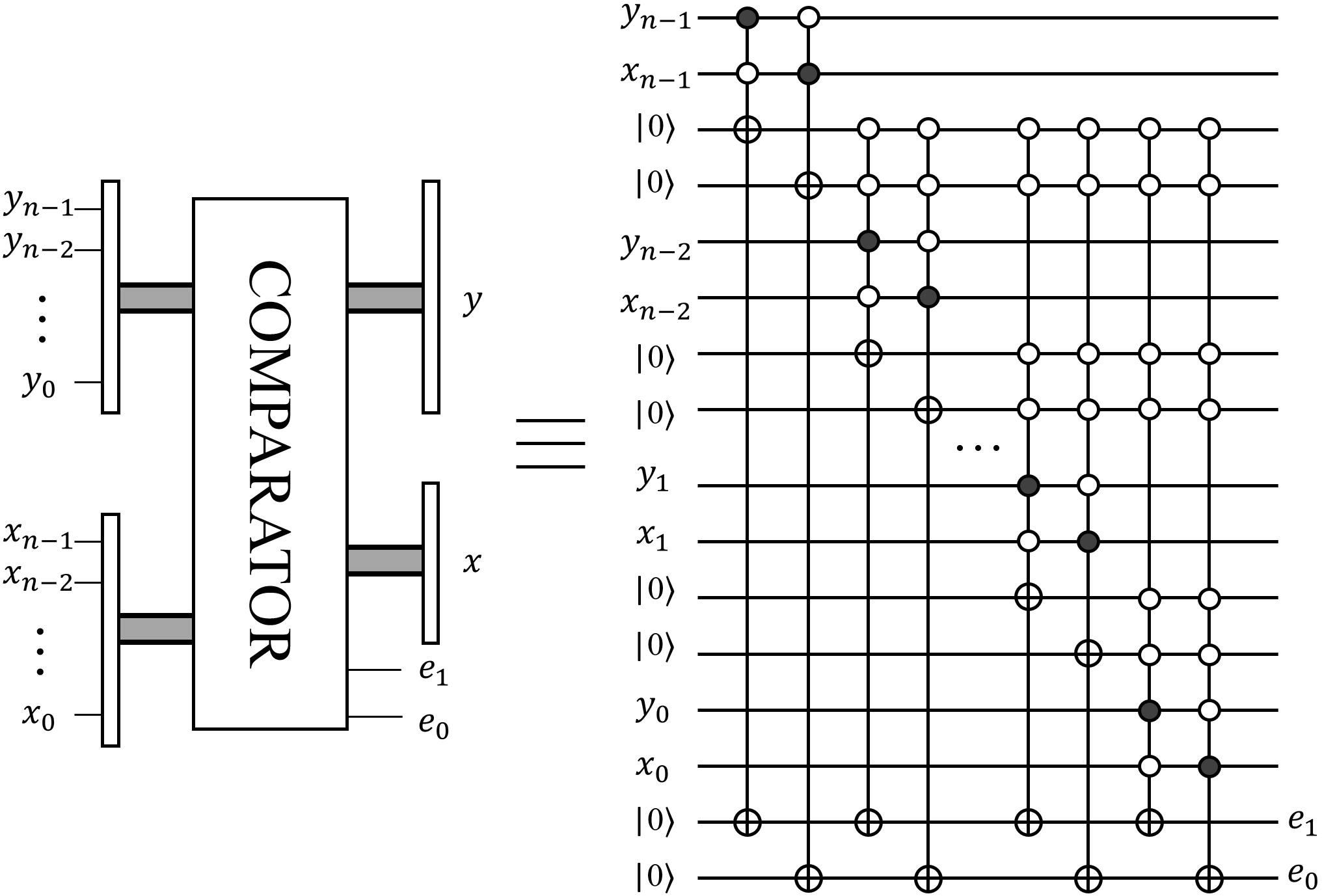
Figure 2: Circuit implementation of quantum COM module (figure and descriptions adapted from [38])

2.4 Quantum accumulator

Since the ghost imaging algorithm requires a series of pixel accumulation operations, we envision the need for circuit network to accumulate these pixels. Hence in this subsection, we present the rudiments for implementing the quantum accumulator (or simply ACC module). Hopefully, the proposed ACC module will be useful for other protocols and applications in the quantum computing domain in general. Mathematically, the ACC module is designed to accomplish the following transformation:

$$\text{ACC}|0\rangle|c_{yx}\rangle|y\rangle|x\rangle=\Big{[}\sum_{y=0}^{2^{n}-1}\sum_{x=0}^{2^{n}-1}|c_{yx}\rangle\Big{]}|c_{yx}\rangle|y\rangle|x\rangle.$$ (3)

As presented in Figure 3, $|y\rangle$ and $|x\rangle$, i.e. $|y_{n-1}y_{n-2}\ldots y_{0}\rangle$ and $|x_{n-1}x_{n-2}\ldots x_{0}\rangle$, are 2n control qubits of the ADD modules, while $|c_{yx}\rangle$ (which includes l qubits) stays different state in each pair of $|y_{i}x_{i}\rangle$. The $|y_{i}x_{i}\rangle$ ranges from $|0^{\otimes 2n}\rangle$ to $|1^{\otimes 2n}\rangle$, i.e. from $|0\rangle$ to $|2^{2n}-1\rangle$. The $2^{2n}$ ADD modules are utilized to perform the summation of $|c_{yx}\rangle$ in each state of $|y_{i}x_{i}\rangle$. The additional l qubits (which are initialized as $|0^{\otimes l}\rangle$) are integrated into the circuit to record the accumulation result of each ADD module, and the combination of these results will be the final output of the whole procedure.

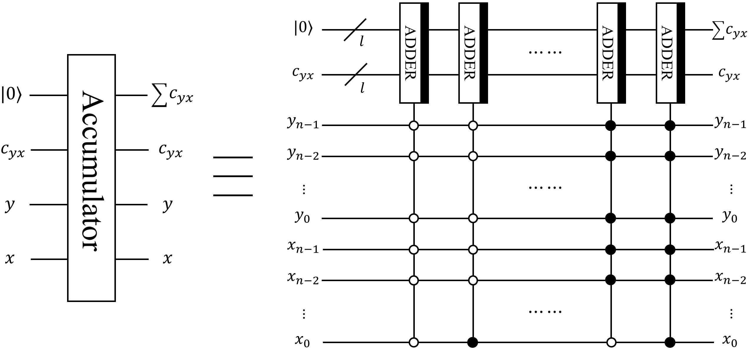
Figure 3: Circuit implementation of quantum ACC module

2.5 Quantum multiplier

Quantum multiplier (i.e. MUL module) is primarily targeted at executing the multiplication operation between two quantum states. Some often-used MUL operations include those in [34] and [36]. In this subsection, although formulated for widespread use, it is designed to support efficient implementation of our proposed QGI protocol. As a premise, we start with the classical multiplication of two binary numbers $y=y_{m-1}\ldots y_{1}y_{0}$ and $x=x_{n-1}\ldots x_{1}x_{0}$. The calculation process is outlined in Eq. (4):

$$yx = (y_{m-1}\ldots y_{1}y_{0})x_{0}+(y_{m-1}\ldots y_{1}y_{0}0)x_{1}$$ (4)

$$+\ldots+(y_{m-1}\ldots y_{1}y_{0}\overbrace{0\ldots 0}^{n-1})x_{n-1}$$

$$= yx_{0}+(y0)x_{1}+\ldots+(y\overbrace{0\ldots 0}^{n-1})x_{n-1}$$

.

To elucidate, let $y=10101$ (i.e. n=5) and $x=1011$ (i.e. $x_{3}=1,x_{2}=0,x_{1}=1,x_{0}=1$, and m=4), then $yx=(10101)\times(1011)=11100111$. The execution of this operation can be better comprehended via the stepwise implementation in Eq. (5).

$$10101\times 1011 = \sum_{i=0}^{3}(2^{i}y)(x_{i})$$ (5)

$$= (2^{0}y)(x_{0})+(2^{1}y)(x_{1})+(2^{2}y)(x_{2})+(2^{3}y)(x_{3})$$

$$= (\overbrace{10101}^{y}\overbrace{\cdot}^{m-4=0})\overbrace{(1)}^{x_{0}}+(\overbrace{10101}^{y}\overbrace{0}^{m-3=1})\overbrace{(1)}^{x_{1}}$$

$$+(\overbrace{10101}^{y}\overbrace{00}^{m-2=2})\overbrace{(0)}^{x_{2}}+(\overbrace{10101}^{y}\overbrace{000}^{m-1=3})\overbrace{(1)}^{x_{3}}$$

$$= 10101+101010+10101000=11100111.$$

Employing the ADD module (presented in Subsection 2.2) and Eq. (4), our proposed MUL operation is executed using Eq. (6):

$$\text{MUL}|0\rangle|z\rangle|y\rangle|x\rangle=|yx\rangle|y\overbrace{0\ldots 0}^{m-1}\rangle|y\rangle|x\rangle,$$ (6)

where a sequence of $|0\rangle$ is used as input to record the product result of $|y\rangle$ and $|x\rangle$, while $|z\rangle$ (including m+n-1 qubits) is used to store the temporary results in the multiplication process. The circuit for implementing MUL module is presented in Figure 4, which is a concatenation of m ADD operators. The procedure of the MUL circuit that computes the result of two binary number multiplication is shown as follows:

(i) Input: Besides the input states of $|y\rangle$ and $|x\rangle$, additional qubits of $|z\rangle$ and $|p\rangle$ (which include m+n-1 and n qubits, respectively) are initialized as a sequence of $|0\rangle$, wherein, $|p\rangle$ is used to dynamically store the intermediate result of the multiplication in each step, while $|z\rangle$ is used to prepare inputs of the ADD module as explained in the sequel.

(ii) Iterative addition: During the (i+1)th step, n Toffoli gates [controlled by the $|y\rangle$ and $|x_{i}\rangle,(i=0,1,\dots m-1)$] are applied on the state of $|z\rangle$ to obtain a result $|z\rangle=|y0^{\otimes i}x_{i}\rangle$ which is regarded as an input for the ADD module (i.e. $\text{ADD}_{i+1}$) in this step, while the other input of $\text{ADD}_{i+1}$ comes from the addition result of $\text{ADD}_{i}$ (it is initialized as $|0^{\otimes n}\rangle$ when i=0).

For instance, in Step 1 (i.e. i=0), if $|x_{0}\rangle=|1\rangle$, we set $|z_{n-1}\ldots z_{1}z_{0}\rangle=|y_{n-1}\ldots y_{1}y_{0}\rangle$, so $|z\rangle=|y\rangle$ in this case. Then, $|z\rangle$ and $|p\rangle$ (p=0) are considered as two inputs of the $\text{ADD}_{1}$. Following the addition operation, n Toffoli gates are employed to reset $|z\rangle$ to its original states, i.e. $|0^{\otimes m+n-1}\rangle$.

Step 3: Output: An iterative approach is used to compute the product between of $|y\rangle$ and $|x\rangle$ (including m+n qubits) such that $|p\rangle=|p_{(m+n-1)}\ldots p_{1}p_{0}\rangle=|y\rangle|x_{0}\rangle+|y0\rangle|x_{1}\rangle+\ldots+|y0^{\otimes{m-2}}\rangle|x_{m-2}\rangle+|y0^{\otimes{m-1}}\rangle|x_{m-1}\rangle$.

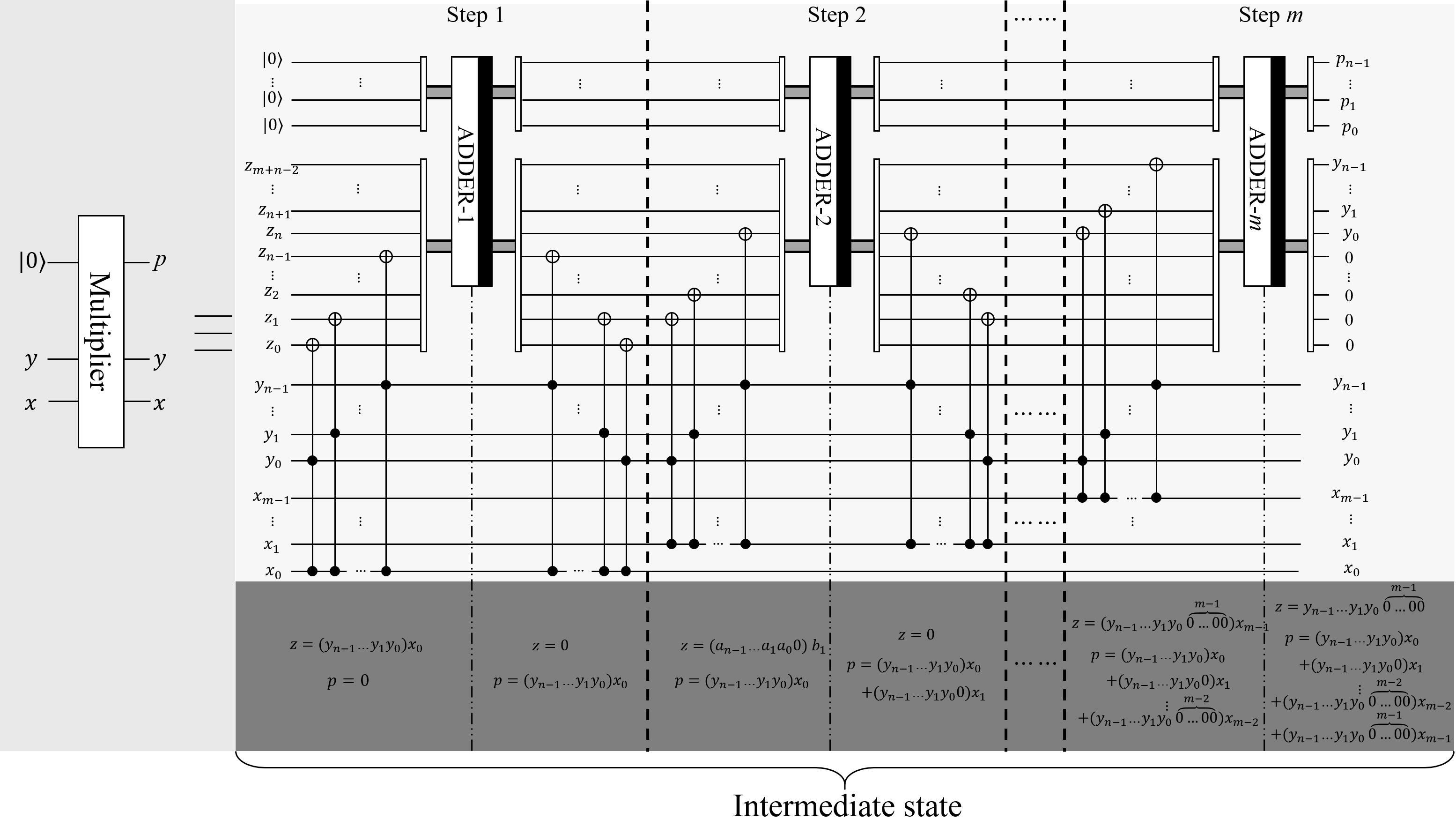
Figure 4: Circuit implementation of quantum MUL module.

2.6 Quantum divider

On classical computers, the binary division operation is actually a series of subtraction tasks. Consider, as an example, the classical division operation “$\frac{100110}{110}$” (as presented in Figure 5), which can be executed via the following 4 steps:

Step 1: A set of the first three bits in the numerator (i.e. the dividend) “100” is taken as minuend in this step, which is used to compare with the denominator (i.e. the divisor) “110” using the COM module (as presented in Subsection 2.3). Since $100<110$, the subtraction operation is not applicable. Therefore, the result of the Step 1 becomes “100” with the next bit in the numerator (in this case “1”) making a sequence “1001” as the new minuend sequence.

Step 2: The two binary sequences being compared, in this step, are the outcome from Step 1 (i.e. “1001”) and the denominator (i.e. “110”). Since $110<1001$, the SUB module (as presented in Section 2.2) will be applied to perform the subtraction. The result of this subtraction “11” and the next bit in the numerator sequence (i.e. “1”) would then serve as the minuend (i.e. “111”) in the next step of the operation.

Step 3: Like in the previous steps, we compare two states using the COM module. However, in this case, the minuend resulting from Step 2 (i.e. “111”) is compared with the divisor (i.e. “110”). Since $111>110$, we proceed with the subtraction $111-110=01$. Finally, the last bit of the numerator (i.e. “0”) is juxtaposed with the outcome of this subtraction to form “010”, which will serve as the minuend for the next step of the operation.

Step 4: Similarly, we compare the minuend “010” with the divisor “110”, and since $010<110$, the subtraction operation is not activated. Having exhausted the bits in the numerator sequence, our operation returns the last two bits of the minuend “10” as the reminder of the division operation. In the event of the opposite scenario, i.e. the minuend is greater than or equal to “110”, the SUB operation is used to obtain the difference that serves rest of the division operation.

As outlined in the four steps above, the division “$\frac{100110}{110}$” produces a quotient “110” and a remainder of “10”. Figure 6 presents a pictorial implementation of the four steps outlined earlier. Based on them, we propose a quantum divider (i.e. DIV module) to implement the division operation.

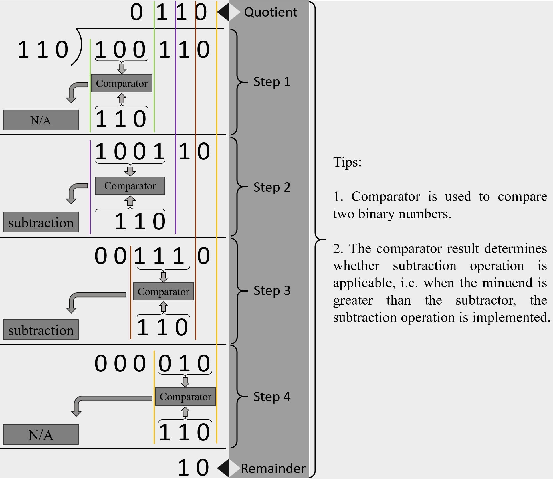
Figure 5: Illustration of the binary division operation.

An overview of the composition, formulation, and circuitry to implement the quantum DIV module that executes the division operation is presented forthwith. Consider a sequence $|y\rangle=|y_{m-1}\ldots y_{1}y_{0}\rangle$ as the dividend (numerator) and another one $|x\rangle=|x_{n-1}\ldots x_{1}x_{0}\rangle$ as the divisor (denominator) of a division operation. Then, using a depository, additional information $|x^{\prime}\rangle=|x^{\prime}_{m-1}\ldots x^{\prime}_{1}x^{\prime}_{0}\rangle$ emanating from the stepwise execution of the subtraction operation (itself part of the quantum DIV operation) to divide $|y\rangle$ by $|x\rangle$, the result of which (i.e. quotient) is recorded as $|q\rangle=|q_{m-n+1}\ldots q_{1}q_{0}\rangle$.

As presented in Step 1 of the DIV circuit (in Figure 6), the first n CNOT gates are used to map the state of $|x_{n-1}\ldots x_{1}x_{0}\rangle$ to $|x^{\prime}_{m-1}x^{\prime}_{m-2}\ldots x^{\prime}_{m-n}\rangle$. Subsequently, the COM module (presented earlier in Subsection 2.3) is utilized to compare between states $|y_{m-1}\ldots y_{1}y_{0}\rangle$ and $|x^{\prime}_{m-1}x^{\prime}_{m-2}\ldots x^{\prime}_{0}\rangle$. An useful state comes out the COM module is $|e_{0}\rangle$. A result $|e_{0}\rangle=|0\rangle$ (i.e. $|y\rangle\geq|x^{\prime}\rangle$) activates the $e_{0}$-controlled SUB module to obtain the subtraction outcome of $|v_{1}\rangle=|y\rangle$-$|x^{\prime}\rangle$ (as the input of COM module in Step 2). Otherwise, the SUB module is inactive so the outcome remains $|y\rangle$ (See the full illustration at the bottom of Figure 6). Following the SUB module, the 1st $e_{0}$-controlled CNOT gate is applied on $|q_{m-n}\rangle$ to obtain the first (also leftmost) or most significant qubit of the division result (i.e. quotient), while the 2nd CNOT gate ensures $|e_{0}\rangle=|0\rangle$ before entering Step 2. At the end of the Step 1, additional n CNOT gates are similarly used to reset state $|x^{\prime}\rangle$ to its initialized state, i.e. sequence of $|0^{\otimes m}\rangle$ entries, preparatory for its use in Step 2.

In Step 2, the first n CNOT gates assign the value $|0x0^{\otimes{m-n-1}}\rangle$ to qubit $|x^{\prime}\rangle$ for the comparison with the output from Step 1 (i.e. $|v_{1}\rangle$). Similarly, $|e_{0}\rangle=|0\rangle$ indicates $|v_{1}\rangle\geq|x^{\prime}\rangle$ so that the subtraction operation will be executed producing an outcome $|v_{2}\rangle=|v_{1}\rangle-|x^{\prime}\rangle$. Following that, the next (n+2) CNOT gates are applied to (1) obtain the 2nd qubit of the division result, (2) assure $|e_{0}\rangle=|0\rangle$ in the next step, and (3) reset $|x^{\prime}\rangle$ from $|0x0^{\otimes{m-n-1}}\rangle$ to $|0^{\otimes m}\rangle$. The final outcome of the DIV module (indicated as $|q\rangle$ at the end of the circuit) is the iterative execution of the steps enumerated above. Meanwhile, the sequence $|v_{m-n+1}\rangle=|v_{m-n}\rangle-|x^{\prime}\rangle$ (technically, composed of $|r_{n-1}r_{n-2}\ldots r_{0}\rangle$ at the end of the circuit) is regarded as the remainder from the DIV operation.

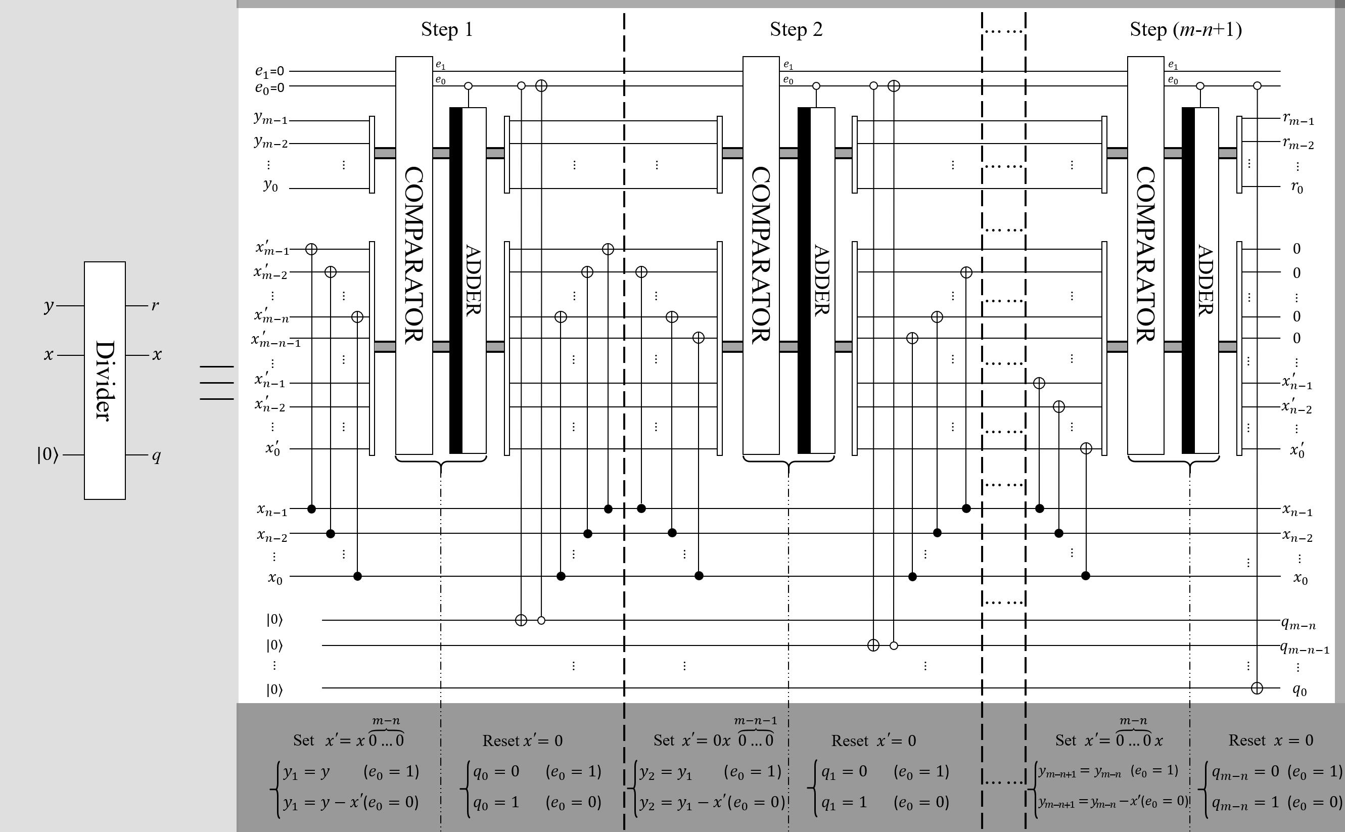
Figure 6: Circuit implementation of quantum DIV module.

3 Circuit-model implementation of ghost imaging experiment

3.1 Mathematical formulation of ghost imaging

Following the mathematical discussions in [7], the methodical outline of our proposed quantum ghost imaging experiment is described in Figure 7. There are two speckle pattern sequences, i.e. $I_{2^{s}-1}^{g}I_{2^{s}-2}^{g}\ldots I_{k}^{g}\ldots I_{1}^{g}I_{0}^{g}$ and $I_{2^{s}-1}^{d}I_{2^{s}-2}^{d}\ldots I_{k}^{d}\ldots I_{1}^{d}I_{0}^{d}$, wherein, $I_{k}^{g}$ and $I_{k}^{d}$ indicate the speckle patterns in the signal and idler fields, respectively. The speckle patterns at the same position of two sequences are identical and each pattern consists of $2^{m}\times 2^{n}$ pixels in the region of $\mathbb{U}$. $\mathbb{U}_{k}(y,x)$ represents a pixel whose coordinate is (y,x) at the kth sample pattern (i.e. $I_{k}^{g}$ in the signal field) in the sequence, where $y\in\{0,1,\ldots,2^{m}-1\}$, $x\in\{0,1,\ldots,2^{n}-1\}$, and $k\in\{0,1,\ldots,2^{s}-1\}$. We define a subregion $\mathbb{A}$ of $\mathbb{U}$, where $\mathbb{A}\subseteq\mathbb{U}$, i.e. the pixels in $\mathbb{A}$ are subset of pixels in $\mathbb{U}$. Furthermore, we define a characteristic function $\mathcal{F}_{k}(y,x)$ in the region $\mathbb{U}$, if $\mathbb{U}_{k}(y,x)$ is in the sub-region $\mathbb{A}$, then $\mathcal{F}_{k}(y,x)=1$; otherwise $\mathcal{F}_{k}(y,x)=0$.

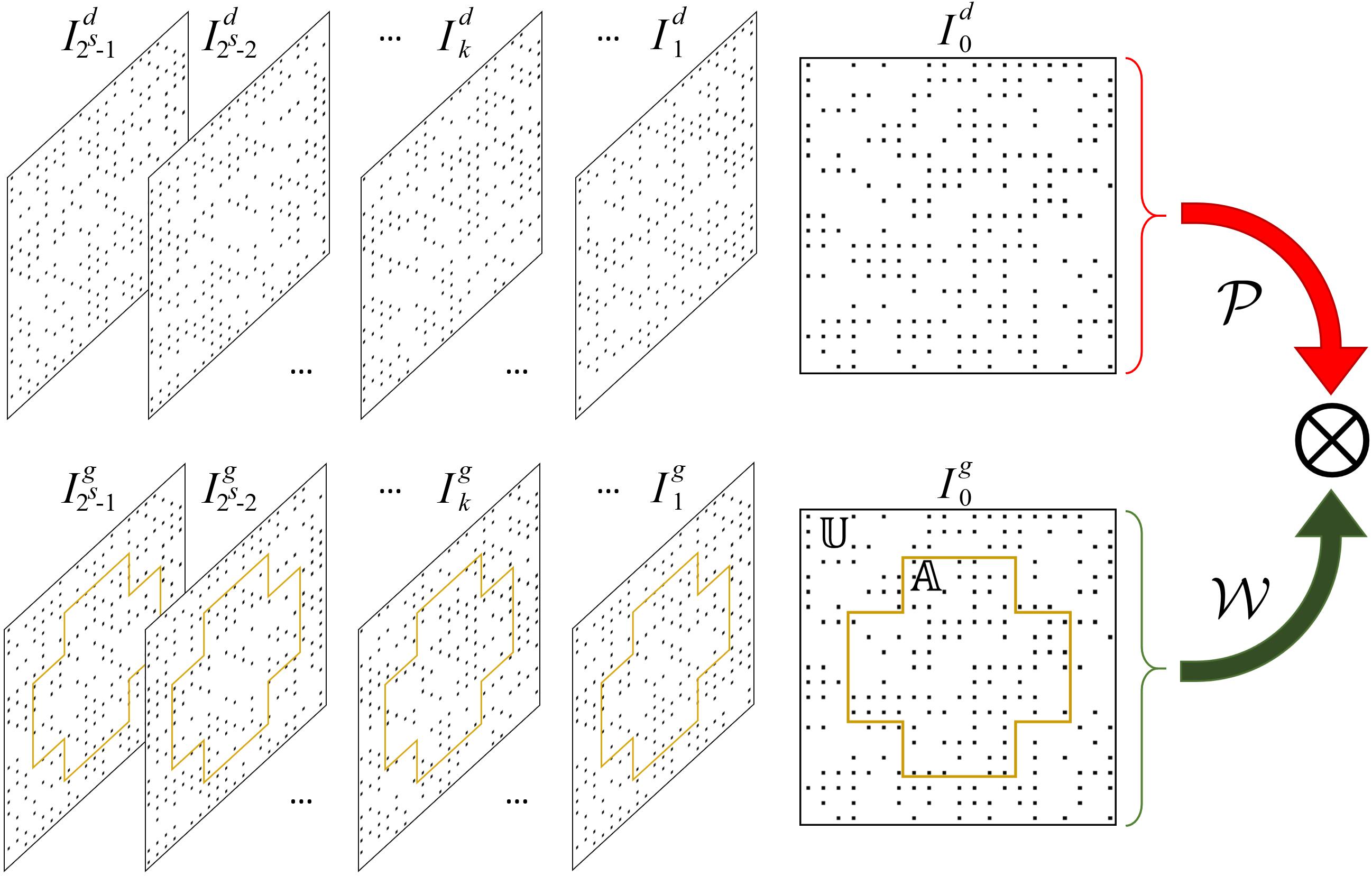
Figure 7: Mathematical analysis of the setups of ghost imaging experiment.

We define a special vector $\mathcal{W}(k)$ whose kth element records the statistical weight for the kth speckle pattern in the sequence (in the signal field). Formally, $\mathcal{W}(k)$ could be calculated as:

$$\mathcal{W}(k)=\sum_{y=0}^{2^{m}-1}\sum_{x=0}^{2^{n}-1}\mathcal{F}_{k}(y,x)\mathbb{U}_{k}(y,x),\ \ \ \ \ (k=0,1,\ldots,2^{s}-1).$$ (7)

where $\mathcal{W}(k)$ calculates the sum of pixels belonging to $\mathbb{A}$ in kth speckle pattern. It represents the weight of the kth speckle pattern in the signal field in the ghost imaging experiment. While $\mathcal{P}$ (in Figure 7) indicates the sequence of speckle patterns that are obtained from the idler field. “$\bigotimes$” in Figure 7 performs cross-correlation operation between the speckle patterns $\mathcal{P}$ and their statistical weights $\mathcal{W}$, after which, the ghost imaging result $\mathcal{R}$ is obtained in the form formulated in Eq. (8):

$$\mathcal{R}=\langle\mathcal{W}\mathcal{P}\rangle-\langle\mathcal{W}\rangle\langle\mathcal{P}\rangle,$$ (8)

where $\langle\cdot\rangle=\frac{1}{2^{s}-1}\sum_{k}\cdot$ denotes an ensemble average over $2^{s}-1$ phase realizations. Meanwhile, every pixel in $\mathcal{R}$ (e.g., at coordinate $(y,x)$) could be represented as:

$$\mathcal{R}(y,x)=\frac{1}{2^{s}-1}\sum_{k=0}^{2^{s}-1}\mathcal{W}_{k}\mathcal{P}_{k}(y,x)-\frac{1}{2^{s}-1}\sum_{k=0}^{2^{s}-1}\mathcal{W}_{k}\cdot\frac{1}{2^{s}-1}\sum_{k=0}^{2^{s}-1}\mathcal{P}_{k}(y,x).$$ (9)

The remainder of this section dwells on the quantum circuit implementation of ghost imaging based on the formulations and discussions presented in Eq. (7)-(9) as well as earlier sections of the study.

3.2 Establishment of quantum speckle patterns

A speckle pattern is defined as a quantum image as presented in Eq. (1) (where l=1), i.e. the chromatic information of every pixel in the speckle pattern only includes two levels, i.e. 0 (black) or 1 (white). It is randomly generated by utilizing the Hadamard gate, i.e. $H=\frac{1}{\sqrt{2}}\small\begin{pmatrix}1&&1\\ -1&&1\end{pmatrix}$, that could transform the initial state $|0\rangle$ to $\frac{1}{\sqrt{2}}(|0\rangle+|1\rangle)$. The whole procedure is outlined in the circuit in Figure 8. It is noteworthy that, whereas on classical computers, the randomness of the gray value is generated with a certain periodicity (i.e. it is pseudo-random), by utilizing the quantum gates (Hadamard and CNOT gates), real-random of speckle patterns can be generated on the quantum computing paradigm.

Moreover, as presented in Figure 8, all $|0\rangle$ initial states are transferred into the outcome of the speckle pattern, which consists of $|s\rangle=|s_{t-1}s_{t-2}\ldots s_{0}\rangle=|0\rangle^{\otimes t}$, $|y\rangle=|y_{m-1}y_{m-2}\ldots y_{0}\rangle=|0\rangle^{\otimes m}$, and $|x\rangle=|x_{n-1}x_{n-2}\ldots x_{0}\rangle=|0\rangle^{\otimes n}$ (all together $m+n+t$ qubits), while an additional qubit $|c_{yx}\rangle$ is employed to record the gray value of every pixel in these patterns. The transformation starts by applying a cortege of Hadamard gates on every qubit of $|0\rangle^{\otimes m+n+t}$, i.e. $\mathcal{H}=H^{\otimes m}\otimes H^{\otimes n}\otimes H^{\otimes t}$ on $|0\rangle^{\otimes m+n+t}=|0\rangle^{\otimes m}\otimes|0\rangle^{\otimes n}\otimes|0\rangle^{\otimes t}$, as formulated in Eq. (10):

$$\mathcal{H}(|0\rangle^{\otimes m+n+t}) = \frac{1}{2^{(m+n+t)/2}}(\overbrace{|0\ldots 00\rangle}^{(m+n+t)\text{qubits}}+\overbrace{|0\ldots 01\rangle}^{(m+n+t)\text{qubits}}+\ldots+\overbrace{|1\ldots 11\rangle}^{(m+n+t)\text{qubits}})$$ (10)

$$= \frac{1}{2^{(m+n+t)/2}}(\sum_{y=0}^{2^{m}-1}|y\rangle\otimes\sum_{x=0}^{2^{n}-1}|x\rangle\otimes\sum_{s=0}^{2^{t}-1}|s\rangle).$$

After the processing in Eq. (10), the initial state has been transformed to an intermediate state, which represents a sequence of speckle patterns ($2^{t}$ patterns) where each pattern is a $2^{m}\times 2^{n}$ quantum image. Finally, a Hadamard gate is utilized on the chromatic wire to assign a binary value to every pixel in the series of speckle patterns. Upon executing Eq. (10), the initial state has been transformed to an intermediate state that evolves into the final speckle pattern composed of states $|y\rangle$, $|x\rangle$, $|s\rangle$, and $|c_{yx}\rangle$ as shown in Figure 8.

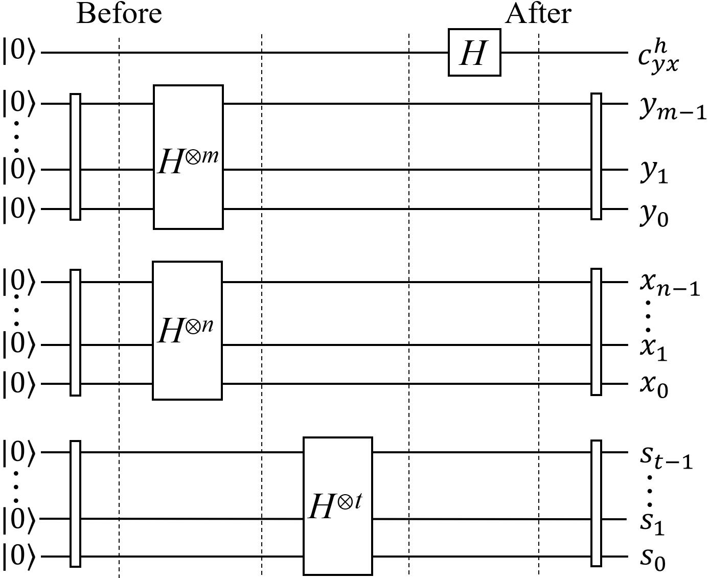
Figure 8: Circuit realization of the quantum speckle patterns.

3.3 Quantum circuit for ghost imaging experiment

Ghost imaging is a technique that is focused on producing an image of an object by combining information from two other sources. In photonic quantum computing, implementation of ghost imaging involves the use of source of pairs of entangled photons and each pair is shared between the two detectors. Since the outcome of Section 3.1, our QIP-based circuit model for implementing QGI could be construed by referring to Eq. (8). Consequently, we tailor our QGI in terms of using quantum computing resources to compute the parameters ($\langle\mathcal{W}\mathcal{P}\rangle$, $\langle\mathcal{W}\rangle$, $\langle\mathcal{P}\rangle$, and $\langle\mathcal{W}\mathcal{P}\rangle-\langle\mathcal{W}\rangle\langle\mathcal{P}\rangle$) in Eq. (8).

3.3.1 Calculation of $\langle\mathcal{W}\mathcal{P}\rangle$ and its circuit implementation

In quantum information and quantum computing, circuit is an effective and pictorial description to the quantum state evolution from the inputs to its outputs. The calculation of $\langle\mathcal{W}\mathcal{P}\rangle$ is detailed in the remainder of this subsection, we outline the execution of the five stages of the quantum circuit implementation of the QGI as presented in Figure 9.

(i)

Interaction between the speckle patterns and phase mask
As delineated in blue rectangle in Figure 9, this unit specifies the interaction between the speckle patterns and the phase mask so as to obtain the quantum interested image (i.e. $|I_{i}\rangle$). The qubit sequence $|y_{m-1}\ldots y_{1}y_{0}\ x_{n-1}\ldots x_{1}x_{0}\ c_{yx}^{m}\rangle$ at the top of this unit represents the quantum phase mask, wherein $|y\rangle$ and $|x\rangle$ are the coordinates, while $|c_{yx}^{m}\rangle$ records the gray value of the pixel in the quantum mask image. The extra qubits, i.e. $|y\rangle$, $|x\rangle$, $|s\rangle$, and $|c_{yx}^{s}\rangle$, represent a series of speckle patterns, where $|s\rangle$ indicates the number of the patterns, and $|y\rangle$ as well as $|x\rangle$ is the pixel coordinates of the pattern, while $|c_{yx}^{s}\rangle$ represents the gray value of pixels in these speckle patterns. In addition, $|c_{yx}^{i}\rangle$ records the gray value that the patterns across the mask image, i.e. the generated quantum interested quantum image.

To realize the needed interaction between the quantum mask image and the quantum speckle pattern, as discussed in Subsection 3.1, a position-wise correspondence comparison between the pixels at the same position of the quantum mask image and each quantum speckle pattern is required. To do this, we have to judge the gray values of the two pixels (i.e. $|c_{yx}^{m}\rangle$ and $|c_{yx}^{s}\rangle$), if both of them are $|1\rangle$, the gray value of the pixel in the interested image (i.e. $|c_{yx}^{i}\rangle$) is transformed from its initialized state $|0\rangle$ to $|1\rangle$ by using a CNOT gate (with multiple control conditions). Otherwise, the gray value of the pixel in the interested image remains $|0\rangle$ (i.e. black). The control conditions imposed on the $|y\rangle$ and $|x\rangle$ coordinates of the quantum mask image are identical with those in the quantum speckle pattern to ensure the operation happens at the same position of them.

(ii)

Calculation of the weight $\bm{|w_{s}\rangle}$ in the signal field
The second unit of our circuit (with yellow legend) accumulated the weights of all the pixels of each quantum interested image. The quantum ACC module presented in Subsection 2.4 is used to undertake this task. The qubit sequence $|y\rangle$ and $|x\rangle$ as well as $|c_{yx}^{i}\rangle$ are regarded as three inputs of the ACC module, while $|w_{s}\rangle=\sum_{y=0}^{2^{m}-1}\sum_{x=0}^{2^{n}-1}|c_{yx}^{i}\rangle$ is the output to store the weight value of every quantum interested image. The control qubits applied on the ACC module in Figure 9 assure that the pixel accumulation happens within the same interested image, i.e. the weight $|w_{s}\rangle$. After the accumulation operation, the output of this part is $|s^{w}w_{s}\rangle$ which contains all the weights of each quantum interested image.

(iii)

Calculation of the product of weights and speckle patterns
The third unit of our circuit (highlighted in green) is used to compare the product of weights ($|w_{s}\rangle$ in the signal field) and the sequence of speckle patterns in the idler filed ($|I_{d}\rangle$) which are not interacted with the mask. The quantum MUL module presented in Subsection 2.5 is used to perform the calculation. The two inputs of the MUL module are the weights of the signal field $|w_{s}\rangle$ and $|c_{yx}^{s}\rangle$ (i.e. the chromatic information of $|I_{d}\rangle$). Meanwhile, $|w_{s}\rangle$ should be multiplied with all the pixels of a speckle pattern ($|I_{k}^{d}\rangle$) in the sequence. The control condition operation on $|s^{w}\rangle$ and $|s\rangle$ confine the operation in the same pairs in the multiplication process (i.e. each $|w_{s}\rangle$ corresponds to each $|I_{k}^{d}\rangle$). The outcome is stored in $|c_{yx}^{s}\rangle=|c_{yx}^{s}\rangle|w_{s}\rangle$ and used as the input of the next unit.

(iv)

Accumulation of the corresponding pixels in the speckle pattern sequence
At the top of the part in purple color, a quantum ACC module is used. The inputs of ACC module are $|c_{yx}^{s}\rangle$ and $|s\rangle$, while the output is stored in $|c_{yx}^{p}\rangle$. The purpose of this unit is to simultaneously accumulate scale of all the pixels’ gray value in the same position of each pattern (in the sequence). The control condition on $|y\rangle$ and $|x\rangle$ ensure that the ACC module is restricted to the same position-wise concurrence in each pattern.

(v)

Calculation of the final result $|\langle w_{s}p_{s}\rangle\rangle$
The chromatic information of the speckle patterns in the idler field, i.e. $|c_{yx}^{p}\rangle$, has been turned to $|w_{s}p_{s}\rangle$ after $2^{2n}$ accumulation operation from the last part. The main task of this part is to change the $|w_{s}p_{s}\rangle$ to $|\langle w_{s}p_{s}\rangle\rangle$, i.e. the ensemble average over $|s\rangle$ phase realizations of $|w_{s}p_{s}\rangle$. Using the DIV module proposed in Subsection 2.6, the state $|w_{s}p_{s}\rangle$ could be divided by $|s\rangle$ to obtain the final result, i.e. $|\langle w_{s}p_{s}\rangle\rangle$.

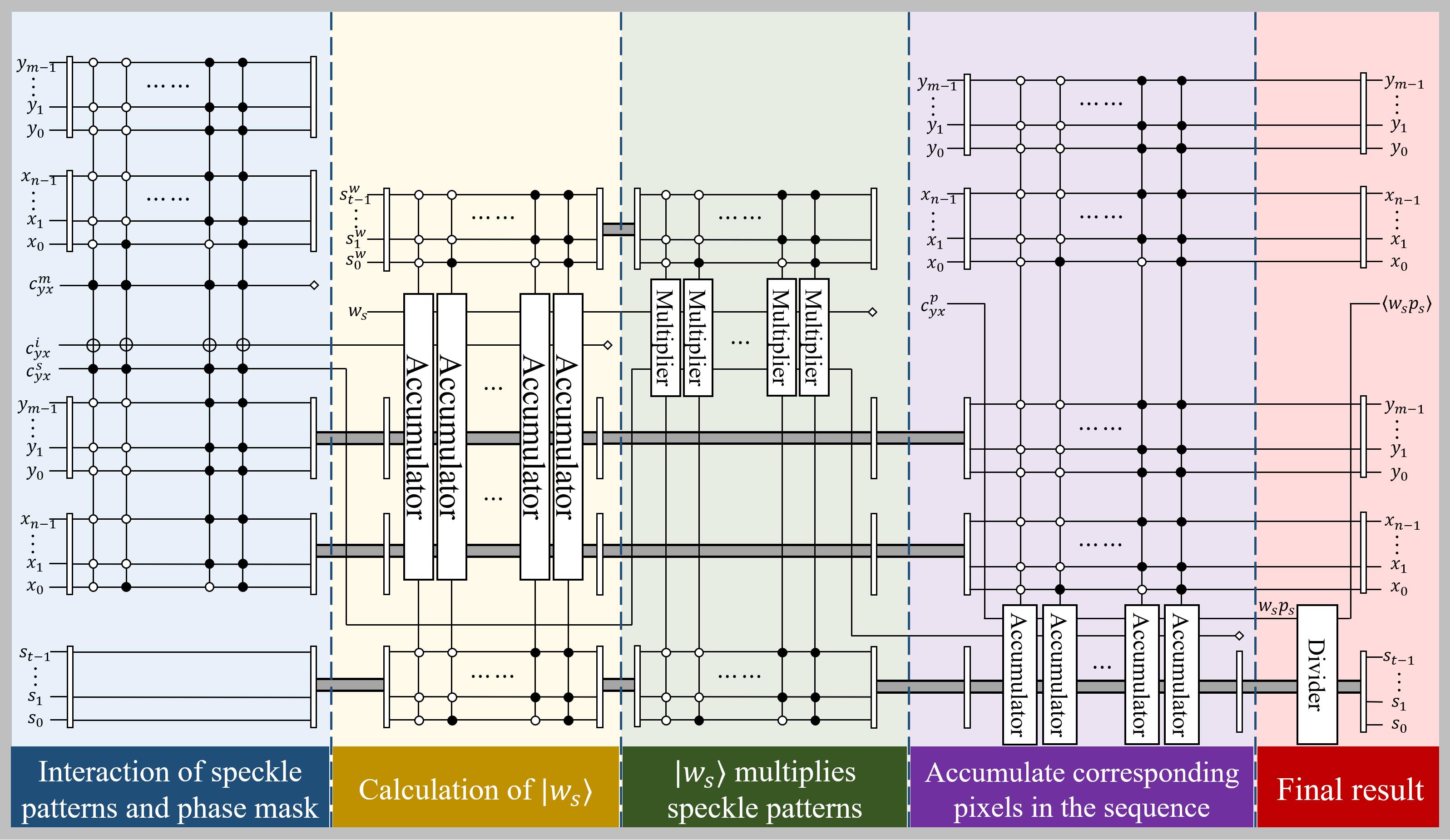
Figure 9: Circuit realization of $|\langle w_{s}p_{s}\rangle\rangle$.

3.3.2 Calculation of $|\langle\mathcal{P}\rangle\rangle$ and $|\langle\mathcal{W}\rangle\rangle$ and their circuit implementations

The calculation circuit of $|\langle p_{s}\rangle\rangle$ is shown in Figure 10(a). The $|yxc_{yx}^{p}\rangle$ is initialized as $\sum_{y=0}^{2^{m}-1}|y\rangle\otimes\sum_{x=0}^{2^{n}-1}|x\rangle\otimes|0\rangle$ which stores the final result $|\langle p_{s}\rangle\rangle$. In addition, $|c_{yx}^{s}yxs\rangle$ represents the quantum speckle patterns which is created by the circuit as shown in Figure 8 and its state is equal to the state $|c_{yx}^{s}yxs\rangle$ as shown in Figure 9. The concurring chromatic information of each pixel ($|c_{yx}^{s}\rangle$) at the same position in $2^{s}$ speckle patterns are accumulated using ACC module and its result would be stored in the state of $|p_{s}\rangle$. Meanwhile, $2^{2n}$ control qubits combinations guarantee concordance in terms of the content of these patterns. In addition, $|p_{s}\rangle$ is the input of DIV module to calculate the final result, i.e. $|\langle p_{s}\rangle\rangle=|p_{s}\rangle/|s\rangle$.

Figure 10(b) outlines the calculation circuit of $|\langle w_{s}\rangle\rangle$ as well as its discussions. The interaction between the speckle patterns and the quantum mask image, and the calculation of $|w_{s}\rangle$ utilizing $2^{m}$ ACC modules own the same process procedures with Figure 9 in blue and yellow color. In addition, $|w_{s}\rangle$ is a superposition state of $2^{m}$ states corresponding to each state of $|s^{w}\rangle$. The ACC module in the last unit (highlighted in red rectangle) is used to aggregate all the $|w_{s}\rangle$ states. Finally, The accumulation result is divided by $|s\rangle$ to calculate the final result, i.e. $|\langle w_{s}\rangle\rangle$.

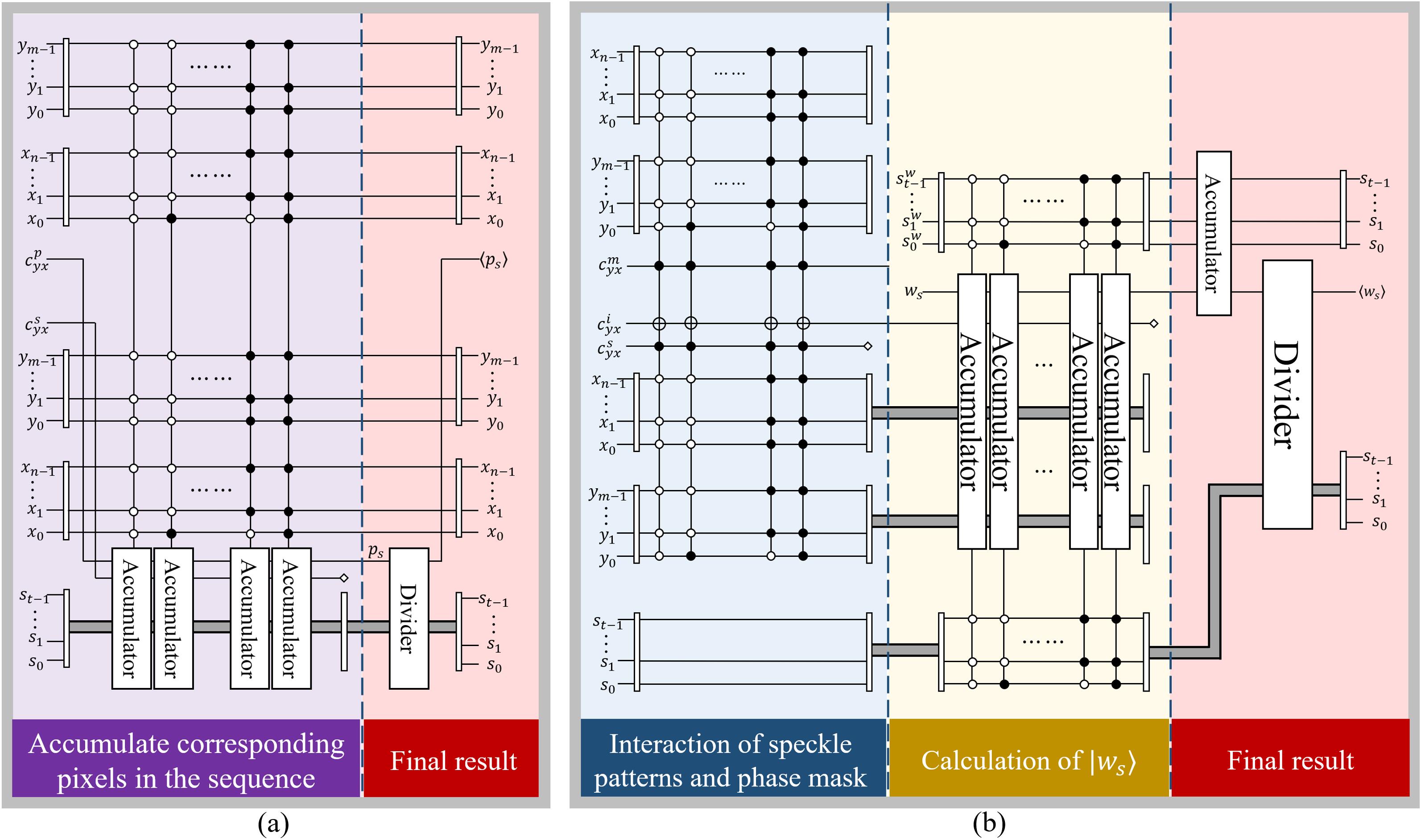
Figure 10: Circuit realization of (a) $|\langle p_{s}\rangle\rangle$ and (b) $|\langle w_{s}\rangle\rangle$.

3.3.3 Creation of the ghost image by using $|\mathcal{R}\rangle=|\langle\mathcal{W}\mathcal{P}\rangle\rangle-|\langle\mathcal{W}\rangle\rangle|\langle\mathcal{P}\rangle\rangle$

By concatenating the various sub-circuits presented in this section, we realize the circuit to implement the ghost imaging technique which also translates to the operation $|\mathcal{R}\rangle=|\langle\mathcal{W}\mathcal{P}\rangle\rangle-|\langle\mathcal{W}\rangle\rangle|\langle\mathcal{P}\rangle\rangle$ (that is $|\langle r_{s}\rangle\rangle=|\langle w_{s}p_{s}\rangle\rangle-|\langle w_{s}\rangle\rangle|\langle p_{s}\rangle\rangle$ as presented in Figure 11). It is trivial that $|\langle w_{s}\rangle\rangle$ and $|\langle p_{s}\rangle\rangle$ are the two inputs of the MUL module and the calculation of them has been discussed in Subsection 3.3.1. The SUB module executes the subtraction operation, but before it, a COM module (whose output is $|e_{0}\rangle$) is set in Figure 11. If $|e_{0}\rangle=|1\rangle$ which means the subtrahend is larger than or equal to minuend, i.e. $|\langle w_{s}\rangle\langle p_{s}\rangle\rangle\geq|\langle w_{s}p_{s}\rangle\rangle$, and the SET-0 operation is triggered. SET-0 operation could set all input qubits to $|0\rangle$ state by using a sequence of CNOT gates (as used in [39]). In such instances, $|e_{0}\rangle$ becomes a control qubit of the ADD module. It is noteworthy that only when $|e_{0}\rangle=|0\rangle$, the ADD module is activated. After $2^{2n}$ comparisons, SET-0, and addition operations, the final result $|\langle r_{s}\rangle\rangle=|\langle w_{s}p_{s}\rangle\rangle-|\langle w_{s}\rangle\rangle|\langle p_{s}\rangle\rangle$ is obtained. The state $|yx\langle r_{s}\rangle\rangle$ is akin the quantum representation of ghost image.

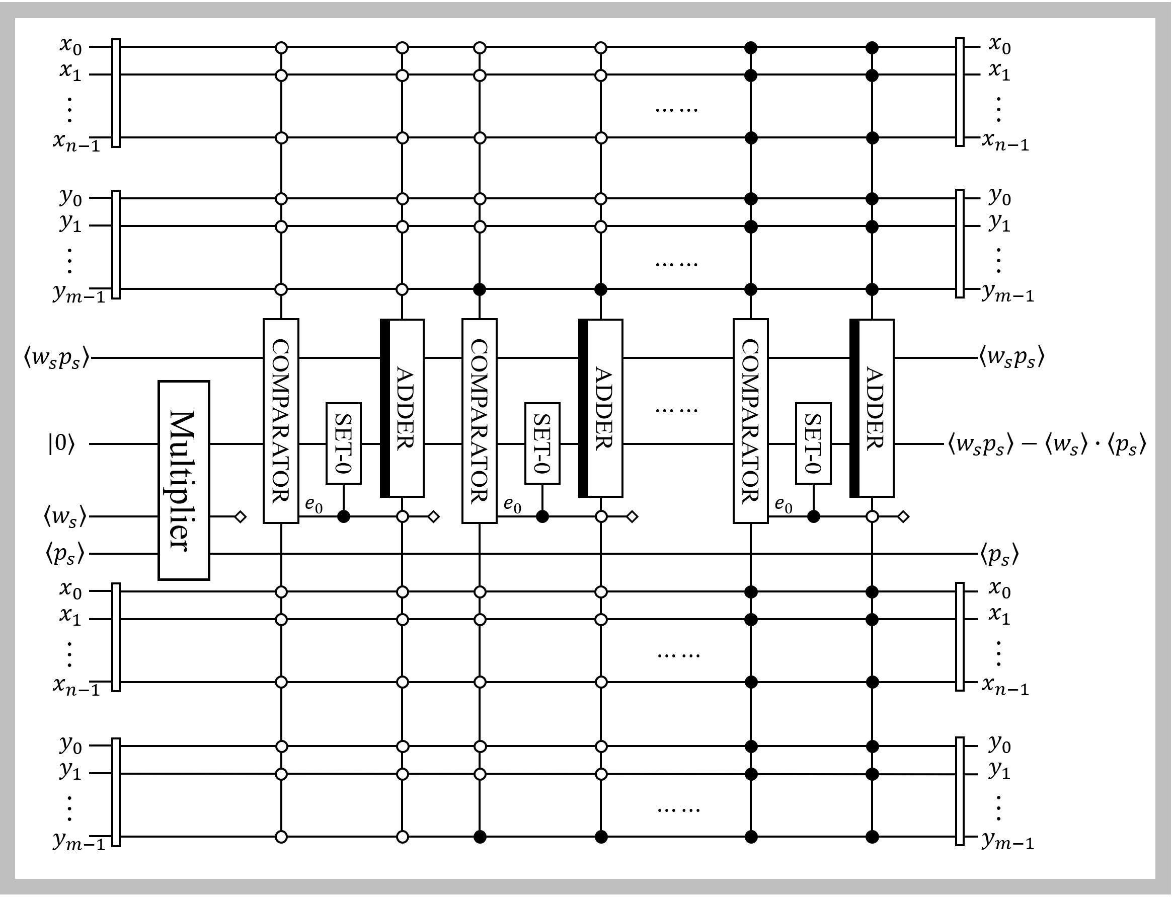
Figure 11: Circuit realization of QGI protocol $|\langle w_{s}p_{s}\rangle\rangle-|\langle w_{s}\rangle\rangle|\langle p_{s}\rangle\rangle$.

4 Conclusions

In this study, we proposed a method to implement the ghost imaging experiment by utilizing the quantum circuit. To achieve this, quantum accumulator (ACC), quantum multiplier (MUL), and quantum divider (DIV) modules were proposed. The contributions in this study mainly include: (1) By utilizing the quantum superposition, in quantum register, the capacity to store quantum speckle patterns was enhanced. In addition, by employing the quantum gates (i.e. Hadamard and CNOT gates), a real random speckle pattern sequence was generated, from which the ghost imaging quality was improved by adjusting the sampling rate of the speckle patters. (2) By utilizing the quantum parallelism, some universal quantum arithmetic modules (such as ACC, MUL, and DIV modules) were designed with low computational complexity so that the ghost imaging speed could be assured. Hopefully, such optimized modules would be applicable for other protocols and applications in the quantum computing domain.

Our future work will focus on the following aspects. First, as introduced in the paper, the quantum mask image only includes binary levels for every pixel, i.e $|0\rangle$ or $|1\rangle$, which is a strong astriction for the ghost imaging technique as well as its applications. Therefore, the extension of its chromatic information becomes an important focus in the following studies. Second, it is practical to find a quantum compressive sensing algorithm whose application on the ghost imaging will explore quantum single-pixel imaging via the compressive sampling. Since the ghost imaging usually requires a large number of speckle patterns, such an algorithm may improve the efficiency when a high quality image is obtained in the proposed ghost imaging protocol. Finally, our proposed ghost imaging protocol could be extended to the application of quantum image encryption. Since the inherent properties of ghost imaging, i.e. neither of the two beams in the signal and idler fields carries the information from the object, it is anticipated that the proposed protocol may offer an outstanding performance for the quantum image encryption.

References

- [1] D. Kazakov, M. Piccardo, W. Y., Self-starting harmonic frequency comb generation in a quantum cascade laser, Nature Photonics 11 (2017) 789–792.
- [2] H. Takenaka, A. Carrasco-Casado, F. M., Satellite-to-ground quantum-limited communication using a 50-kg-class microsatellite, Nature Photonics 11 (2017) 502–508.
- [3] M. Hush, Machine learning for quantum physics, Science 355 (2017) 580.
- [4] A. Trabesinger, Quantum computing: towards reality, Nature 543 (2017) S1.
- [5] R. Boyd, P. Reynolds, Introduction to the special issue on quantum imaging, Quantum Information Processing 11 (2012) 887–889.
- [6] S. Venegas-Andraca, Introductory words: special issue on quantum image processing published by quantum information processing, Quantum Information Processing 14 (2015) 1535–1537.
- [7] L. Basano, P. Ottonello, A conceptual experiment on single-beam coincidence detection with pseudothermal light, Optics Express 15 (19) (2007) 12386–12394.
- [8] B. Erkmen, J. Shapiro, Ghost imaging: from quantum to classical to computational, Advances in Optics and Photonics 2 (2010) 405–450.
- [9] T. Pittman, Y. Shih, D. Strekalov, A. Sergienko, Optical imaging by means of two-photon quantum entanglement, Physical Review A 52 (1995) R3429.
- [10] R. Bennink, B. S.J., R. Boyd, two-photon coincidence imaging with a classical source, Physical Review Letters 89 (11) (2002) 113601.
- [11] A. Gatti, M. Bondani, L. Lugiato, Comment on “can two-photon correlation of chaotic light be considered as correlation of intensity fluctuations?”, Physical Review Letters 98 (2007) 039301.
- [12] G. Scarcelli, V. Berardi, Y. Shih, Scarcelli, berardi, and shih reply (to the comment by a. gatti et al.), Physical Review Letters 98 (2007) 039302.
- [13] Y. Shih, The physics of ghost imaging-nonlocal interference or local intensity fluctuation correlation?, Quantum Information Processing 11 (2012) 995–1001.
- [14] J. Shapiro, B. R., Response to “the physics of ghost imaging-nonlocal interference or local intensity fluctuation correlation?”, Quantum Information Processing 11 (2012) 1003–1011.
- [15] R. Schneider, T. Mehringer, M. G., Quantum imaging with incoherently scattered light from a free-electron laser, Nature Physics 14 (2018) 126–129.
- [16] J. Tetienne, N. Dontschuk, D. Broadway, Quantum imaging of current flow in graphene, Science Advances 3 (2017) e1602429.
- [17] R. Feynman, Simulating physics with computers, International journal of theoretical physics 21 (6-7) (1982) 467–488.
- [18] P. Shor, Algorithms for quantum computation: discrete logarithms and factoring, in: Proceedings of the 35th Annual Symposium on Foundations of Computer Science, 1994, pp. 124–134.
- [19] D. Deutsch, Quantum theory, the church-turing principle and the universal quantum computer, in: Proceedings of the Royal Society of London A 400, 1985, pp. 97–117.
- [20] A. Iliyasu, Towards realising secure and efficient image and video processing applications on quantum computers, Entropy 15 (2013) 2874–2974.
- [21] N. Abura’ed, F. Khan, H. Bhaskar, Advances in the quantum theoretical approach to image processing applications, ACM Computing Surveys 49 (4) (2017) 75.1–75.49.
- [22] F. Yan, A. Iliyasu, P. Le, Quantum image processing: a review of advances in its security technologies, International Journal of Quantum Information 15 (2017) 1730001.
- [23] F. Yan, A. Iliyasu, S. Venegas-Andraca, A survey of quantum image representations, Quantum Information Processing 15 (1) (2016) 1–35.
- [24] S. Venegas-Andraca, S. Bose, Storing, processing, and retrieving an image using quantum mechanics, in: Proceedings of SPIE Conference of Quantum Information and Computation, Vol. 5105, 2003, pp. 134–147.
- [25] P. Le, F. Dong, K. Hirota, A flexible representation of quantum images for polynomial preparation, image compression, and processing operations, Quantum Information Processing 10 (1) (2011) 63–84.
- [26] N. Jiang, J. Wang, Y. Mu, Quantum image scaling up based on nearest-neighbor interpolation with integer scaling ratio, Quantum Information Processing 14 (2015) 4001–4026.
- [27] H. Li, Q. Zhu, R. Zhou, M. Li, L. Song, Multidimensional color image storage, retrieval, and compression based on quantum amplitudes and phases, Information Sciences 273 (2014) 212–232.
- [28] X. Yao, W. H., L. Z., Quanum image processing and its application to edge detection: theory and experiment, Pysical Review X 7 (2017) 031041.
- [29] S. Caraiman, V. Manta, Histogram-based segmentation of quantum images, Theoretical Computer Science 529 (2014) 46–60.
- [30] A. Iliyasu, P. Le, F. Dong, K. Hirota, Watermarking and authentication of quantum images based on restricted geometric transformations, Information Sciences 186 (1) (2012) 126–149.
- [31] R. Zhou, W. Hu, F. P., Quantum realization of the bilinear interpolation method for neqr, Scientific Reports 7 (2017) 2511.
- [32] F. Yan, A. Iliyasu, S. Venegas-Andraca, A survey of quantum image representations, Quantum Information Processing 15 (1) (2016) 1–35.
- [33] Y. Zhang, K. Lu, Y. Gao, M. Wang, Neqr: a novel enhanced quantum representation of digital images, Quantum Information Processing 12 (8) (2013) 2833–2860.
- [34] V. Vlatko, B. Adriano, E. Artur, Quantum networks for elementary arithmetic operations, Physical Review A 54 (1) (1996) 147–153.
- [35] T. Draper, Addition on a quantum computer, arXiv:quant-ph/0008033.
- [36] F. Yan, K. Chen, S. Venegas-Andraca, J. Zhao, Quantum image rotation by an arbitrary angle, Quantum Information Processing 16 (282).
- [37] D. Wang, Z. Liu, W. Zhu, S. Li, Design of quantum comparator based on extended general toffoli gates with multiple targets, Computer Science 39 (9) (2012) 302–306.
- [38] F. Yan, A. Iliyasu, H. Yang, K. Hirota, Strategy for quantum image stabilization, Science China Information Sciences 59 (2016) 052102.
- [39] K. Chen, F. Yan, A. Iliyasu, J. Zhao, Exploring the implementation of steganography protocols on quantum audio signals, International Journal of Theoretical Physics 57 (2) (2018) 476–494.