Feedback pinning control of collective behaviors aroused by epidemic spread on complex networks

Pan Yang Zhongpu Xu Jianwen Feng Xinchu Fu xcfu@shu.edu.cn Department of Mathematics, Shanghai University, Shanghai 200444, China College of Mathematics and Statistics, Shenzhen University, Shenzhen 518060, China
Abstract

This paper investigates epidemic control behavioral synchronization for a class of complex networks resulting from spread of epidemic diseases via pinning feedback control strategy. Based on the quenched mean field theory, epidemic control synchronization models with inhibition of contact behavior is constructed, combining with the epidemic transmission system and the complex dynamical network carrying extra controllers. By the properties of convex functions and Gerschgorin theorem, the epidemic threshold of the model is obtained, and the global stability of disease-free equilibrium is analyzed. For individual’s infected situation, when epidemic spreads, two types of feedback control strategies depended on the diseases’ information are designed: the one only adds controllers to infected individuals, the other adds controllers both to infected and susceptible ones. And by using Lyapunov stability theory, under designed controllers, some criteria that guarantee epidemic control synchronization system achieving behavior synchronization are also derived. Several numerical simulations are performed to show the effectiveness of our theoretical results. As far as we know, this is the first work to address the controlling behavioral synchronization induced by epidemic spreading under the pinning feedback mechanism. It is hopeful that we may have more deeper insight into the essence between disease’s spreading and collective behavior controlling in complex dynamical networks.

keywords:
Epidemic model; Control behavioral synchronization; Pinning feedback control; Complex network

1 Introduction

Complex networks are ubiquitous around the world, such as the World Wide Web, biological networks, food chain networks, power grids and transportation networks, economic and social networks, see [1]-[10] and references therein. Since complex networks can be used as models to reflect certain intrinsic natures in the real world, a lot of achievements have been made on complex networks [11, 12]. Synchronization and propagation, two typical interesting and important dynamical behaviors in networks, have attracted much attention from various fields in recent years, including communication, engineering, physical science, mathematics, sociology and biology. On the one hand, many kinds of synchronization mechanisms have been discovered over the last decades, such as the complete synchronization [13, 14], the cluster synchronization [15, 16], the lag synchronization [17, 18], and so on, see [19]-[21] and references therein. On the other hand, the spreading of epidemic disease in complex networks have also been received more and more attentions due to the development of network science research since 1998. When an epidemic disease spreads in a realistic network, the information about the disease transfer only along the edges, which means that there will no direct transmission in any pairs of individuals without relationship between them. Taking into consideration of the significance about spreading of epidemic diseases on complex networks, many successful works have been devoted by a lot of researchers from mathematical biology field [22]-[24]. The problem about global stability and attractivity of a network-based SIS epidemic model with nonmonotone incidence rate was investigated in [25], and the conditions guaranteeing global asymptotical stability or global attractivity of an endemic equilibrium are also obtained. And the issue of network-level reproduction number and extinction threshold for vector-borne diseases was studied in [26], meanwhile relationships between the basic reproduction numbers and the extinction thresholds of corresponding models are obtained by using some assumptions.

One may think that collective behaviors and spreading behaviors are two independent patterns of behavior in complex networks, however, the fact seem to be not the case. In fact, when an epidemic disease spreads in a network, individuals always change their behaviors to protect themselves from being infected by infected individuals around them. They may take steps consistently, such as washing their hands with soaps frequently, having the cure in hospital, avoiding going to the crowded and doing exercise to strengthen their resistance to infection, and so on, to combat the disease. These consistent behaviors against the epidemic disease are also called as behavior synchronization induced by contagious diseases. There are some successful works in recent years [27]-[30] taking the synchronization and epidemic transmission in complex networks into consideration simultaneously. Motivated by these interesting works, in this paper, we will further study the problem about the behavior synchronization induced by epidemic spread.

In [31], authors considered adaptive mechanism between dynamical synchronization and epidemic spreading behavior on complex networks, in which two models of epidemic synchronization were introduced for the first time to analyze the stability of epidemic synchronization and obtained local and global conditions. Following that, the interplay between collective behavior and spreading dynamics on complex networks was further investigated in [32], where several bidirectional networks models of spreading phenomena were constructed, and found that the collective behavior and spreading behavior are influenced each other. But the models in the above two papers are all based on the heterogeneous mean-field theory. In order to be more accurate in predicting epidemic synchronization, authors in [33] introduced the quenched mean-field theory to construct three epidemic synchronization models without delays or with distinct delays, and got some local and global conditions to guarantee the results. Therefore, the quenched mean-field theory will be also considered in our work for more precise prediction of epidemic collective behaviors. However, models in these works are all about adaptive synchronization with adaptive exterior coupling strength. As is known to all, it is relatively difficult to synchronize a network only depending on itself evolution. Hence, we will add external controllers to achieve behavioral synchronization aroused by the epidemic disease transmission in this work.

It is acknowledged that adding external controllers to reach synchronization is an important and effective method in a scale-large complex network [34]-[36]. When an epidemic disease breaks out, it is also important to actively control collective behaviors, as the individuals may not get full information about the diseases or even do not know the event of contagion in the early stage. Therefore, in order to make individuals in a network response quickly in the early stage of an epidemic disease spreading, some external controlling methods are carried out to reach behavioral consistency for the individuals, named as controlling behavioral synchronization induced by epidemic disease transmission. Such control can be performed via broadcasting and other media of information dissemination or some certain well-directed means, by which individuals may consistently behavior, such as going to the hospital, washing their hands with soaps, etc., to protect themselves from being infected, and resist the diffusion of contagions. As far as we know, there are no works concerning epidemic behavior synchronization via a control strategy. Therefore, we will discuss the collective behaviors induced by epidemic disease transmission in the view of external pinning feedback controller introduced in [34] with the normalized outer-coupling strength in the synchronous models. The difference in this case is that the pinning feedback controllers depend upon the information about epidemic spreading, where controllers work only when contagious disease spreads. In addition, noticing a realistic fact that there are always the inhibition of contact behaviors among individuals rooted in the subconscious, especially when an contagion spreads. In other words, individuals may change their willing to contact with others relying on the risk of being infected, and the consistency with the behavioral target resulting from protecting themselves, which can be reflected as the higher of the risk of being infected, the less the individuals are willing to contact with each other. And the less distinct between behavioral targets, persons are desired to touch with others. Thus it is natural to consider the inhibition of contact behavior into our models.

Inspired by the above discussions, this paper further studies the the pinning feedback control of behavior synchronization induced by epidemic diseases spreading. The outer-coupling strength is normalization and the external pinning feedback controllers are equipped in the synchronous models. And in the epidemic spreading models, the quenched mean-field theory is introduced for more accurate reflection of the realistic situations, and more precise evaluation of the control behavior synchronization aroused from transmission of contagious. What’s more, in order to simulate more real human reaction, the inhibition of contact behaviors are also considered in our epidemic spreading models. That is to say, on the one hand, the higher the risk of being infected, the less the willing to contact with each other. On the other hand, the more consistent the individuals’ behaviors are, the stronger the desires to keep in touch. We will use distinct pinning feedback control strategies to achieve corresponding control of behavior synchronization, which means the corresponding controllers will be added to only a portion of nodes or individuals for each strategy in the network.

The main contributions of this work are listed as follows. Firstly, combined with the synchronous systems and Susceptible-Infected-Susceptible (SIS) epidemic systems, based on the quenched mean-field theory, we construct a class of models of epidemic controlled behavioral synchronization with the external controllers, in which the outer-coupling strength is normalized in the synchronous system. Secondly, in order to perform more real simulation, the inhibition of contact behavior is concerned in the epidemic system, which means that the desires to contact with others not only rely on the risk of being infected, but also depend on the difference between behavioral target states. Finally, pinning feedback control are equipped into the epidemic synchronization for the first time. In other words, only a part of nodes will be controlled by corresponding feedback strategies, and the controllers are related to the information of the epidemic spread, which means the controllers will work only when the epidemic spreads, or failures with the epidemic extinction.

The rest of the paper is organized as follows. In Section 2, the problem is formulated and some helpful definitions, lemmas, assumptions and notations are given. In Section 3, the existence of endemic equilibrium and the global stability of disease-free equilibrium are analyzed at first in the epidemic controlling synchronization models, and then the theoretical results for distinct controlled behaviors synchronization induced by epidemic spreading under different control strategies are derived. Some numerical examples are shown to illustrate the theoretical results in Section 4. Finally, the conclusions of this paper are presented in Section 5.

Notations.

Throughout the paper, \mathbb{R} is the set of real numbers, nsuperscript𝑛\mathbb{R}^{n} represents the n𝑛n dimensional Euclidean space, +nsuperscriptsubscript𝑛\mathbb{R}_{+}^{n} is the n𝑛n dimensional vector space with positive elements, and n×msuperscript𝑛𝑚\mathbb{R}^{n\times m} denotes the set of real matrices with order n×m𝑛𝑚n\times m. The transposition for a vector or a matrix is represented by superscript T𝑇T. λmin()subscript𝜆\lambda_{\min}(\cdot) and λmax()subscript𝜆\lambda_{\max}(\cdot) represent the minimum and maximum eigenvalues of a square matrix, respectively. And INsubscript𝐼𝑁I_{N} is the identity matrix of order N𝑁N. \|\cdot\| represents the Euclidean norm for vectors and the induced 222-norm for matrices. And tensor-product\otimes is the Kronecker product. For a matrix P𝑃P, P>0(<0)𝑃annotated0absent0P>0(<0) means that P𝑃P is positive (negative) definite.

2 Models and Preliminaries

The mathematical models about infectious disease dynamics and complex dynamical network systems are given in this part. And some fundamental conceptions and necessary preliminaries are introduced for later use.

2.1 Mathematical models

A. Complex dynamical network model

We now introduce a coupled complex network with N𝑁N nodes or individuals under controlling

x˙i(t)=f(xi(t))+j=1Naijxj(t)+ui(t),i=1,,N,formulae-sequencesubscript˙𝑥𝑖𝑡𝑓subscript𝑥𝑖𝑡superscriptsubscript𝑗1𝑁subscript𝑎𝑖𝑗subscript𝑥𝑗𝑡subscript𝑢𝑖𝑡𝑖1𝑁\displaystyle\dot{x}_{i}(t)=f(x_{i}(t))+\sum_{j=1}^{N}a_{ij}x_{j}(t)+u_{i}(t),\quad i=1,\cdots,N, (1)

where xi(t)=(xi1(t),,xin(t))Tnsubscript𝑥𝑖𝑡superscriptsubscript𝑥𝑖1𝑡subscript𝑥𝑖𝑛𝑡𝑇superscript𝑛x_{i}(t)=(x_{i1}(t),\cdots,x_{in}(t))^{T}\in{\mathbb{R}^{n}} represents the i𝑖i-th node’s state, f()::𝑓absentf(\cdot): nnsuperscript𝑛superscript𝑛\mathbb{R}^{n}\rightarrow\mathbb{R}^{n} is a differentiable function that represents the behavior of individual system, and f(xi(t))=(f1(xi(t)),f2(xi(t)),,fn(xi(t)))Tn.𝑓subscript𝑥𝑖𝑡superscriptsubscript𝑓1subscript𝑥𝑖𝑡subscript𝑓2subscript𝑥𝑖𝑡subscript𝑓𝑛subscript𝑥𝑖𝑡𝑇superscript𝑛f(x_{i}(t))=(f_{1}(x_{i}(t)),f_{2}(x_{i}(t)),\cdots,f_{n}(x_{i}(t)))^{T}\in\mathbb{R}^{n}. Matrix A=(aij)N×N𝐴subscript𝑎𝑖𝑗superscript𝑁𝑁A=(a_{ij})\in{\mathbb{R}^{N\times N}} represents the out-coupled structure, in which aij=aji=1subscript𝑎𝑖𝑗subscript𝑎𝑗𝑖1a_{ij}=a_{ji}=1 if there is a connection between nodes (or individuals) i𝑖i and j𝑗j, and aij=aji=0subscript𝑎𝑖𝑗subscript𝑎𝑗𝑖0a_{ij}=a_{ji}=0 otherwise. ui(t)subscript𝑢𝑖𝑡u_{i}(t) is the external controller for each node i𝑖i, which will be defined later.

Define the Laplacian matrix as L=(lij)N×N𝐿subscript𝑙𝑖𝑗superscript𝑁𝑁L=(l_{ij})\in{\mathbb{R}^{N\times N}}:

lij=aij,subscript𝑙𝑖𝑗subscript𝑎𝑖𝑗l_{ij}=-a_{ij},
lii=j=1,jiNlij,i=1,2,,Nformulae-sequencesubscript𝑙𝑖𝑖superscriptsubscriptformulae-sequence𝑗1𝑗𝑖𝑁subscript𝑙𝑖𝑗𝑖12𝑁l_{ii}=-\sum_{j=1,j\neq i}^{N}l_{ij},\quad i=1,2,\cdots,N

.

Assume the Laplacian matrix L𝐿L is irreducible, which indicates that network with N𝑁N nodes is strongly connected, e.g., there exists one path from any node i𝑖i to j.𝑗j. From the definition of Laplacian L𝐿L, it is obvious that L𝐿L has one zero eigenvalue and N1𝑁1N-1 positive eigenvalue, which means that there exists a unitary matrix U𝑈U such that

UTLU=diag{λ1,λ2,,λN},superscript𝑈𝑇𝐿𝑈diagsubscript𝜆1subscript𝜆2subscript𝜆𝑁U^{T}LU={\rm diag}\{\lambda_{1},\lambda_{2},\cdots,\lambda_{N}\},

we sort these eigenvalues as 0=λ1λ2λN.0subscript𝜆1subscript𝜆2subscript𝜆𝑁0=\lambda_{1}\leq\lambda_{2}\leq\cdots\leq\lambda_{N}.

B. SIS epidemic dynamics model

Taking into account the network’s topological structure, this paper introduces the following quenched networks for infectious disease systems (or quenched mean field model):

ρ˙i(t)=ρi(t)+λφi(t)[1ρi(t)]j=1Naijρj(t)subscript˙𝜌𝑖𝑡subscript𝜌𝑖𝑡𝜆subscript𝜑𝑖𝑡delimited-[]1subscript𝜌𝑖𝑡superscriptsubscript𝑗1𝑁subscript𝑎𝑖𝑗subscript𝜌𝑗𝑡\displaystyle\dot{\rho}_{i}(t)=-\rho_{i}(t)+\lambda\varphi_{i}(t)[1-\rho_{i}(t)]\sum_{j=1}^{N}a_{ij}\rho_{j}(t) (2a)
S˙i(t)=ρi(t)λφi(t)[1ρi(t)]j=1Naijρj(t)subscript˙𝑆𝑖𝑡subscript𝜌𝑖𝑡𝜆subscript𝜑𝑖𝑡delimited-[]1subscript𝜌𝑖𝑡superscriptsubscript𝑗1𝑁subscript𝑎𝑖𝑗subscript𝜌𝑗𝑡\displaystyle\dot{S}_{i}(t)=\rho_{i}(t)-\lambda\varphi_{i}(t)[1-\rho_{i}(t)]\sum_{j=1}^{N}a_{ij}\rho_{j}(t) (2b)

where ρi(t)subscript𝜌𝑖𝑡\rho_{i}(t) and Si(t)subscript𝑆𝑖𝑡S_{i}(t) represent the infected probability and the uninfected probability of node i𝑖i at time t𝑡t, respectively. λ𝜆\lambda is the infection rate. φi(t)subscript𝜑𝑖𝑡\varphi_{i}(t) is the probability of inhibition to contact behavior for each individual i𝑖i, which has the representation as φi(t)=1γi(t)subscript𝜑𝑖𝑡1subscript𝛾𝑖𝑡\varphi_{i}(t)=1-\gamma_{i}(t), where γi(t)subscript𝛾𝑖𝑡\gamma_{i}(t) is defined as follows,

γi(t)=αρi(t)eiT(t)ei(t)i=1NeiT(t)ei(t),subscript𝛾𝑖𝑡𝛼subscript𝜌𝑖𝑡superscriptsubscript𝑒𝑖𝑇𝑡subscript𝑒𝑖𝑡superscriptsubscript𝑖1𝑁superscriptsubscript𝑒𝑖𝑇𝑡subscript𝑒𝑖𝑡\gamma_{i}(t)=\alpha\rho_{i}(t)\frac{e_{i}^{T}(t)e_{i}(t)}{\sum_{i=1}^{N}e_{i}^{T}(t)e_{i}(t)},

in which α𝛼\alpha denotes the gain of desire for contact, and α(0,1).𝛼01\alpha\in(0,1). And the ei(t)subscript𝑒𝑖𝑡e_{i}(t) is the synchronization errors for the i𝑖i-th node defined later.

Remark 1.

Note that the inhibition to contact behavior is a natural reaction for all the population, especially in the case of breaking out of an epidemic disease. This behavior not only depends on the information about the risk of being infected by other individuals, but also on the target to reach. On the one hand, the greater the risk of being infected is, the weaker the desire to contact with others is. On the other hand, the smaller the behavior error between synchronous target is, the stronger the willing to contact with others is.

C. SIS epidemic controlling synchronization model

Then by combining the SIS epidemic dynamics model and complex dynamical network model, we get the epidemic controlling synchronization model with external controllers:

x˙i(t)=f(xi(t))j=1Nlijxj(t)+ui(t)subscript˙𝑥𝑖𝑡𝑓subscript𝑥𝑖𝑡superscriptsubscript𝑗1𝑁subscript𝑙𝑖𝑗subscript𝑥𝑗𝑡subscript𝑢𝑖𝑡\displaystyle\dot{x}_{i}(t)=f(x_{i}(t))-\sum_{j=1}^{N}l_{ij}x_{j}(t)+u_{i}(t) (3a)
ρ˙i(t)=ρi(t)+λφi(t)[1ρi(t)]j=1Naijρj(t)subscript˙𝜌𝑖𝑡subscript𝜌𝑖𝑡𝜆subscript𝜑𝑖𝑡delimited-[]1subscript𝜌𝑖𝑡superscriptsubscript𝑗1𝑁subscript𝑎𝑖𝑗subscript𝜌𝑗𝑡\displaystyle\dot{\rho}_{i}(t)=-\rho_{i}(t)+\lambda\varphi_{i}(t)[1-\rho_{i}(t)]\sum_{j=1}^{N}a_{ij}\rho_{j}(t) (3b)

This kind of compound model mixes dynamical equation of individual’s state and equation for individual’s spreading of disease, and in the case of the controlling behavioral synchronization induced by the transmission of epidemic disease, xi(t)subscript𝑥𝑖𝑡x_{i}(t) denotes the state variable of the individual (or node) i𝑖i at time t𝑡t in the epidemic disease network, which reflects certain daily behavioral patterns (washing the hands, traveling and having a rest, etc.). ρi(t)subscript𝜌𝑖𝑡\rho_{i}(t) represents the probability of being infected for individual i𝑖i at time t𝑡t. Assume that individuals may be infected only when there exists connections among them. At this moment, model (1) and model (2) share the same topology structure. In other words, the dynamical behaviors of individuals and the epidemic spreading behaviors appear simultaneously in the same network, which indicates that the process of individuals’ dynamical behaviors will accompany the spreading behavior of epidemic disease in the disease network. And the f𝑓f defines the local dynamics that represents the summation of distinct behaviors for epidemic individuals, and the f𝑓f is active, dynamic as well as complex. In this paper, we realize the coupling between the model (1) and model (2) by external controllers depending on the epidemic information of individuals’ disease and the synchronous errors, then reaching the point of controlling behavioral synchronization under the premise of epidemic diseases transmission.

In the first equation of model (3), ui(t)subscript𝑢𝑖𝑡u_{i}(t) represents the external controller for each node i𝑖i consisting of two parts, ρi(t)subscript𝜌𝑖𝑡\rho_{i}(t) and ei(t)subscript𝑒𝑖𝑡e_{i}(t), in which ρi(t)subscript𝜌𝑖𝑡\rho_{i}(t) can be regarded as the information about the epidemic disease for each individual, while the other term is the essential part in the pinning control strategy that measures the synchronous state of each individual (or node). Then the controllers will be activated and play a role according to the situation about the breaking-out of the epidemic disease under this framework for controllers. Which means that the controllers will work to lead the behavioral synchronization when the epidemic disease spreads, e.g., ρi(t)subscript𝜌𝑖𝑡\rho_{i}(t) will not be zero as t𝑡t tends to positive infinity. When the epidemic disease dose not spread, the controllers will be invalid due to the disease’s die out, i.e., ρi(t)subscript𝜌𝑖𝑡\rho_{i}(t) goes to zero. Hence it is no needed to control individuals in the network to get the collective behavior. Thus it is meaningful to design the pinning controllers to relate to ρi(t)subscript𝜌𝑖𝑡\rho_{i}(t).

2.2 Preliminaries

For analytical requirement, some useful preliminaries are introduced in this part.

Definition 1.

A complex dynamical network system containing N𝑁N individuals (or nodes) is said to reach asymptotical synchronization, if for each pair nodes i𝑖i and j𝑗j (ij𝑖𝑗i\neq j) we have

limtxi(t)xj(t)=0.subscript𝑡normsubscript𝑥𝑖𝑡subscript𝑥𝑗𝑡0\lim_{t\rightarrow\infty}\|x_{i}(t)-x_{j}(t)\|=0.

Assume that there exists a synchronous orbit s(t),𝑠𝑡s(t), then it is just needed to check xi(t)s(t)0normsubscript𝑥𝑖𝑡𝑠𝑡0\|x_{i}(t)-s(t)\|\rightarrow 0 as t𝑡t\rightarrow\infty to achieve asymptotical synchronization. As for the case of distinct synchronous orbits sk(t),subscript𝑠𝑘𝑡s_{k}(t), if xi(t)sk(t)0normsubscript𝑥𝑖𝑡subscript𝑠𝑘𝑡0\|x_{i}(t)-s_{k}(t)\|\rightarrow 0 as t,𝑡t\rightarrow\infty, i𝑖i belongs to distinct groups k𝑘k, then the dynamical network achieves cluster synchronization.

Definition 2 ([38]).

A continuous function f(t,x):[0,+]×nn:𝑓𝑡𝑥0superscript𝑛superscript𝑛f(t,x):[0,+\infty]\times\mathbb{R}^{n}\rightarrow\mathbb{R}^{n} is said to be in a QUAD function class, denoted as fQUAD(P,Δ,η)𝑓QUAD𝑃Δ𝜂f\in\mbox{QUAD}(P,\Delta,\eta), if there exists a positive definite diagonal matrix P=diag{p1,p2,,pn},𝑃𝑑𝑖𝑎𝑔subscript𝑝1subscript𝑝2subscript𝑝𝑛P=diag\{p_{1},p_{2},\cdots,p_{n}\}, a diagonal matrix Δ=diag{δ1,δ2,,δn}Δ𝑑𝑖𝑎𝑔subscript𝛿1subscript𝛿2subscript𝛿𝑛\Delta=diag\{\delta_{1},\delta_{2},\cdots,\delta_{n}\} and a constant η>0,𝜂0\eta>0, such that f𝑓f satisfies following condition:

(xy)TP(f(t,x)f(t,y)Δ(xy))η(xy)T(xy)superscript𝑥𝑦𝑇𝑃𝑓𝑡𝑥𝑓𝑡𝑦Δ𝑥𝑦𝜂superscript𝑥𝑦𝑇𝑥𝑦(x-y)^{T}P(f(t,x)-f(t,y)-\Delta(x-y))\leq-\eta(x-y)^{T}(x-y)

for all x,yn.𝑥𝑦superscript𝑛x,y\in\mathbb{R}^{n}.

Remark 2.

Notice a fact that there are many chaotic systems having the properties of the QUAD function class, for example, the Lorenz system, the Rössler system, the Chen system, the Chua’s circuit, and the logistic differential system.

Definition 3.

Matrix L𝐿L is said to be class A1,𝐴1A1, denoted as LA1,𝐿𝐴1L\in A1, if the following conditions hold:

  1. 1.

    lij0,ij,lii=j=1,jiNlij,formulae-sequencesubscript𝑙𝑖𝑗0formulae-sequence𝑖𝑗subscript𝑙𝑖𝑖superscriptsubscriptformulae-sequence𝑗1𝑗𝑖𝑁subscript𝑙𝑖𝑗l_{ij}\leq 0,i\neq j,l_{ii}=-\sum_{j=1,j\neq i}^{N}l_{ij},

  2. 2.

    L𝐿L is irreducible.

If L𝐿L is symmetric, we say L𝐿L belongs to class A2,𝐴2A2, denoted as LA2.𝐿𝐴2L\in A2. We can easily obtain that if L𝐿L is class A1,𝐴1A1, then L𝐿L has the property of zero row-sum, e.g., j=1Nlij=0.superscriptsubscript𝑗1𝑁subscript𝑙𝑖𝑗0\sum_{j=1}^{N}l_{ij}=0.

As for a rectangular matrix LN1×N2,𝐿superscriptsubscript𝑁1subscript𝑁2L\in\mathbb{R}^{N_{1}\times N_{2}}, if its each row-sum is zero, e.g., j=1N2lij=0,i=1,2,,N1,formulae-sequencesuperscriptsubscript𝑗1subscript𝑁2subscript𝑙𝑖𝑗0𝑖12subscript𝑁1\sum_{j=1}^{N_{2}}l_{ij}=0,i=1,2,\cdots,N_{1}, then we call L𝐿L is in class A3,𝐴3A3, denoted as LA3.𝐿𝐴3L\in A3.

Lemma 1 ([39]).

For any vectors x,yn,𝑥𝑦superscript𝑛x,y\in\mathbb{R}^{n}, there exists positive θ,𝜃\theta, such that

2xTy1θxTx+θyTy.2superscript𝑥𝑇𝑦1𝜃superscript𝑥𝑇𝑥𝜃superscript𝑦𝑇𝑦2x^{T}y\leq\frac{1}{\theta}x^{T}x+\theta y^{T}y.
Lemma 2 (Gerschgorin Theorem [40]).

Let A=(aij)n×n𝐴subscript𝑎𝑖𝑗superscript𝑛𝑛A=(a_{ij})\in\mathbb{C}^{n\times n} and let ri=j=1,jin|aij|,i=1,2,,n.formulae-sequencesubscript𝑟𝑖superscriptsubscriptformulae-sequence𝑗1𝑗𝑖𝑛subscript𝑎𝑖𝑗𝑖12𝑛r_{i}=\sum_{j=1,j\neq i}^{n}|a_{ij}|,~{}i=1,2,\cdots,n. Then all the eigenvalues of A𝐴A lie in the union of n𝑛n closed discs i=1n{z:|zaii|ri},superscriptsubscript𝑖1𝑛conditional-set𝑧𝑧subscript𝑎𝑖𝑖subscript𝑟𝑖\bigcup_{i=1}^{n}\{z\in\mathbb{C}:|z-a_{ii}|\leq r_{i}\}, where \mathbb{C} is the set of complex numbers and n×nsuperscript𝑛𝑛\mathbb{C}^{n\times n} represents the complex matrices set of order n×n.𝑛𝑛n\times n.

3 Main Results

The main concern of our study is controlling the behavioral dynamics system  (3) to achieve desired behavior synchronization via designed controller ui(t)subscript𝑢𝑖𝑡u_{i}(t) during the spread of an infectious disease.

The reason to add controllers can be explained as follows. Because of unresponsive information transmission or unawareness about the disease type, when the infectious disease outbreaks, e.g., infection rate is larger than the epidemic threshold, people may not make corresponding response to this case in a short time, or the information about disease is transmitted by medical institutions to the public after some research. At this moment, some guidance or measures should be carried out on their behaviors to reach an identical action, including getting cure in hospital and isolating, or washing hands frequently and having rest and so on, which prevent a disease from next outbreak. Obviously, this kind of behavioral consistency is resulted from the disease transmission, and is achieved under external feedback controllers.

Before analyzing behavior synchronization, the model (2)’s equilibrium will be studied first.

3.1 Analysis of the infectious disease system

Let

𝚪={(ρi,,ρN)+N|0ρi1,i=1,,N}.𝚪conditional-setsubscript𝜌𝑖subscript𝜌𝑁superscriptsubscript𝑁formulae-sequence0subscript𝜌𝑖1𝑖1𝑁\mathbf{\Gamma}={\{(\rho_{i},\cdots,\rho_{N})\in\mathbb{R}_{+}^{N}|0\leq\rho_{i}\leq 1,~{}i=1,\cdots,N\}}.

Obviously, it is easy to know that ΓΓ\Gamma is the positive invariant set for system (2).

Theorem 1.

If the infection rate λ>1(1α)ρ(A)𝜆11𝛼𝜌𝐴\lambda>\frac{1}{(1-\alpha)\rho(A)}, then the epidemic dynamics system (2) has a positive equilibrium E=(S1,ρ1,,SN,ρN),superscript𝐸superscriptsubscript𝑆1superscriptsubscript𝜌1superscriptsubscript𝑆𝑁superscriptsubscript𝜌𝑁E^{*}=(S_{1}^{*},\rho_{1}^{*},\cdots,S_{N}^{*},\rho_{N}^{*}), i.e., the endemic equilibrium.

Proof.

Denote by ρisubscript𝜌𝑖\rho_{i} the steady state of ρi(t)subscript𝜌𝑖𝑡\rho_{i}(t), and let the right-hand side equal to zero in the first one equation (2a) of the system (2), then define

Θ=j=1Naijρj.Θsuperscriptsubscript𝑗1𝑁subscript𝑎𝑖𝑗subscript𝜌𝑗\displaystyle\Theta=\sum_{j=1}^{N}a_{ij}\rho_{j}. (4)

From the system (2), we have

Θ=j=1NaijλφiΘ1+λφiΘ.Θsuperscriptsubscript𝑗1𝑁subscript𝑎𝑖𝑗𝜆subscript𝜑𝑖Θ1𝜆subscript𝜑𝑖Θ\displaystyle\Theta=\sum_{j=1}^{N}a_{ij}\frac{\lambda\varphi_{i}\Theta}{1+\lambda\varphi_{i}\Theta}. (5)

In order to analyze the ΘΘ\Theta’s property, construct the auxiliary function

F(Θ)=Θj=1NaijλφiΘ1+λφiΘ.𝐹ΘΘsuperscriptsubscript𝑗1𝑁subscript𝑎𝑖𝑗𝜆subscript𝜑𝑖Θ1𝜆subscript𝜑𝑖Θ\displaystyle F(\Theta)=\Theta-\sum_{j=1}^{N}a_{ij}\frac{\lambda\varphi_{i}\Theta}{1+\lambda\varphi_{i}\Theta}. (6)

Then, we can get the first-order derivative at ΘΘ\Theta

dF(Θ)dΘ=1j=1Naijλφi(1+λφiΘ)2,𝑑𝐹Θ𝑑Θ1superscriptsubscript𝑗1𝑁subscript𝑎𝑖𝑗𝜆subscript𝜑𝑖superscript1𝜆subscript𝜑𝑖Θ2\displaystyle\frac{dF(\Theta)}{d\Theta}=1-\sum_{j=1}^{N}a_{ij}\frac{\lambda\varphi_{i}}{(1+\lambda\varphi_{i}\Theta)^{2}}, (7)

and the second-order derivative at ΘΘ\Theta

d2F(Θ)dΘ2=j=1Naij2λ2φi2(1+λφiΘ)3>0,superscript𝑑2𝐹Θ𝑑superscriptΘ2superscriptsubscript𝑗1𝑁subscript𝑎𝑖𝑗2superscript𝜆2superscriptsubscript𝜑𝑖2superscript1𝜆subscript𝜑𝑖Θ30\displaystyle\frac{d^{2}F(\Theta)}{d\Theta^{2}}=\sum_{j=1}^{N}a_{ij}\frac{2\lambda^{2}\varphi_{i}^{2}}{(1+\lambda\varphi_{i}\Theta)^{3}}>0, (8)

As for the first-order derivative at Θ=0Θ0\Theta=0, we have

dF(Θ)dΘ|Θ=0evaluated-at𝑑𝐹Θ𝑑ΘΘ0\displaystyle\frac{dF(\Theta)}{d\Theta}\Big{|}_{\Theta=0} =1j=1Naijλφi<1j=1Naijλ(1α).absent1superscriptsubscript𝑗1𝑁subscript𝑎𝑖𝑗𝜆subscript𝜑𝑖1superscriptsubscript𝑗1𝑁subscript𝑎𝑖𝑗𝜆1𝛼\displaystyle=1-\sum_{j=1}^{N}a_{ij}\lambda\varphi_{i}<1-\sum_{j=1}^{N}a_{ij}\lambda(1-\alpha).

Then, it is necessary for the equation F(Θ)=0𝐹Θ0F(\Theta)=0 to have a unique positive solution within the internal (0,1)01(0,1) that the following relation holds

λ>1(1α)j=1Naij,𝜆11𝛼superscriptsubscript𝑗1𝑁subscript𝑎𝑖𝑗\displaystyle\lambda>\frac{1}{(1-\alpha)\sum_{j=1}^{N}a_{ij}}, (9)

and inequality (9) means

λ>1(1α)maxij=1Naij.𝜆11𝛼subscript𝑖superscriptsubscript𝑗1𝑁subscript𝑎𝑖𝑗\displaystyle\lambda>\frac{1}{(1-\alpha)\max_{i}\sum_{j=1}^{N}a_{ij}}. (10)

On the other hand, according to the Gersgorin disc theorem,

|λi(A)|j=1Naij,subscript𝜆𝑖𝐴superscriptsubscript𝑗1𝑁subscript𝑎𝑖𝑗\displaystyle|\lambda_{i}(A)|\leq\sum_{j=1}^{N}a_{ij}, (11)

so we further know that

maxi|λi(A)|maxij=1Naij.subscript𝑖subscript𝜆𝑖𝐴subscript𝑖superscriptsubscript𝑗1𝑁subscript𝑎𝑖𝑗\displaystyle\max_{i}|\lambda_{i}(A)|\leq\max_{i}\sum_{j=1}^{N}a_{ij}. (12)

From the definition of spectral radius for the matrix A𝐴A, we have

ρ(A)=maxi|λi(A)|maxij=1Naij.𝜌𝐴subscript𝑖subscript𝜆𝑖𝐴subscript𝑖superscriptsubscript𝑗1𝑁subscript𝑎𝑖𝑗\displaystyle\rho(A)=\max_{i}|\lambda_{i}(A)|\leq\max_{i}\sum_{j=1}^{N}a_{ij}. (13)

Therefore, by the condition

λ>1(1α)ρ(A),𝜆11𝛼𝜌𝐴\displaystyle\lambda>\frac{1}{(1-\alpha)\rho(A)}, (14)

we obtain the first-order derivative of F(Θ)𝐹ΘF(\Theta)

dF(Θ)dΘ|Θ=0<0.evaluated-at𝑑𝐹Θ𝑑ΘΘ00\displaystyle\frac{dF(\Theta)}{d\Theta}\Big{|}_{\Theta=0}<0.

Then the proof is completed. ∎

It is worthy to notice that Theorem 1 discovers when the infection rate λ>1(1α)ρ(A),𝜆11𝛼𝜌𝐴\lambda>\frac{1}{(1-\alpha)\rho(A)}, there exists ρi(0,1),i=1,2,,Nformulae-sequencesuperscriptsubscript𝜌𝑖01𝑖12𝑁\rho_{i}^{*}\in(0,1),i=1,2,\cdots,N, such that

limtρi(t)=ρi,i=1,2,,N.formulae-sequencesubscript𝑡subscript𝜌𝑖𝑡superscriptsubscript𝜌𝑖𝑖12𝑁\displaystyle\lim_{t\rightarrow\infty}\rho_{i}(t)=\rho_{i}^{*},\quad i=1,2,\cdots,N.

Next, the global stability of disease-free equilibrium will be considered. Some mathematical expressions are given for analytical requirement. Setting the positive left eigenvector corresponding to the maximum eigenvalue of A𝐴A as (ω1,,ωN)TN,superscriptsubscript𝜔1subscript𝜔𝑁𝑇superscript𝑁(\omega_{1},\cdots,\omega_{N})^{T}\in\mathbb{R}^{N}, which indicates that

(ω1,,ωN)A=(ω1,,ωN)ρ(A).subscript𝜔1subscript𝜔𝑁𝐴subscript𝜔1subscript𝜔𝑁𝜌𝐴(\omega_{1},\cdots,\omega_{N})A=(\omega_{1},\cdots,\omega_{N})\rho(A).
Theorem 2.

The disease-free equilibrium in the epidemic dynamics system (2) is globally asymptotically stable if the infection rate λ1(1+α)ρ(A).𝜆11𝛼𝜌𝐴\lambda\leq\frac{1}{(1+\alpha)\rho{(A)}}. While it is unstable when λ>1(1α)ρ(A).𝜆11𝛼𝜌𝐴\lambda>\frac{1}{(1-\alpha)\rho{(A)}}.

Proof.

Choose the following Lyapunov functional

V(t)=i=1Nωiρi(t).𝑉𝑡superscriptsubscript𝑖1𝑁subscript𝜔𝑖subscript𝜌𝑖𝑡\displaystyle V(t)=\sum_{i=1}^{N}\omega_{i}\rho_{i}(t). (15)

Differentiating the function V(t)𝑉𝑡V(t) along the trajectories of Eq. (2), we obtain

V˙(t)˙𝑉𝑡\displaystyle\dot{V}(t) =i=1Nωiρ˙i(t)absentsuperscriptsubscript𝑖1𝑁subscript𝜔𝑖subscript˙𝜌𝑖𝑡\displaystyle=\sum_{i=1}^{N}\omega_{i}\dot{\rho}_{i}(t)
=i=1Nωi[ρi(t)+λφi(t)(1ρi(t))j=1Naijρj(t)]absentsuperscriptsubscript𝑖1𝑁subscript𝜔𝑖delimited-[]subscript𝜌𝑖𝑡𝜆subscript𝜑𝑖𝑡1subscript𝜌𝑖𝑡superscriptsubscript𝑗1𝑁subscript𝑎𝑖𝑗subscript𝜌𝑗𝑡\displaystyle=\sum_{i=1}^{N}\omega_{i}\Big{[}-\rho_{i}(t)+\lambda\varphi_{i}(t)(1-\rho_{i}(t))\sum_{j=1}^{N}a_{ij}\rho_{j}(t)\Big{]}
=i=1Nωiρi(t)+λi=1Nj=1Nωiφi(t)aijρj(t)λi=1Nj=1Nωiρi(t)[1αρi(t)eiT(t)ei(t)i=1NeiT(t)ei(t)]aijρj(t)absentsuperscriptsubscript𝑖1𝑁subscript𝜔𝑖subscript𝜌𝑖𝑡𝜆superscriptsubscript𝑖1𝑁superscriptsubscript𝑗1𝑁subscript𝜔𝑖subscript𝜑𝑖𝑡subscript𝑎𝑖𝑗subscript𝜌𝑗𝑡𝜆superscriptsubscript𝑖1𝑁superscriptsubscript𝑗1𝑁subscript𝜔𝑖subscript𝜌𝑖𝑡delimited-[]1𝛼subscript𝜌𝑖𝑡superscriptsubscript𝑒𝑖𝑇𝑡subscript𝑒𝑖𝑡superscriptsubscript𝑖1𝑁superscriptsubscript𝑒𝑖𝑇𝑡subscript𝑒𝑖𝑡subscript𝑎𝑖𝑗subscript𝜌𝑗𝑡\displaystyle=-\sum_{i=1}^{N}\omega_{i}\rho_{i}(t)+\lambda\sum_{i=1}^{N}\sum_{j=1}^{N}\omega_{i}\varphi_{i}(t)a_{ij}\rho_{j}(t)-\lambda\sum_{i=1}^{N}\sum_{j=1}^{N}\omega_{i}\rho_{i}(t)\Big{[}1-\alpha\rho_{i}(t)\frac{e_{i}^{T}(t)e_{i}(t)}{\sum_{i=1}^{N}e_{i}^{T}(t)e_{i}(t)}\Big{]}a_{ij}\rho_{j}(t)
[λ(1+α)ρ(A)1]ωρ,absentdelimited-[]𝜆1𝛼𝜌𝐴1𝜔𝜌\displaystyle\leq\Big{[}\lambda(1+\alpha)\rho(A)-1\Big{]}\omega\rho,

where ω=(ω1,,ωN)TN,𝜔superscriptsubscript𝜔1subscript𝜔𝑁𝑇superscript𝑁\omega=(\omega_{1},\cdots,\omega_{N})^{T}\in\mathbb{R}^{N}, ρ=(ρ1(t),,ρN(t))TN.𝜌superscriptsubscript𝜌1𝑡subscript𝜌𝑁𝑡𝑇superscript𝑁\rho=(\rho_{1}(t),\cdots,\rho_{N}(t))^{T}\in\mathbb{R}^{N}.

Therefore, if λ1(1+α)ρ(A)𝜆11𝛼𝜌𝐴\lambda\leq\frac{1}{(1+\alpha)\rho{(A)}}, we have V˙(t)0˙𝑉𝑡0\dot{V}(t)\leq 0, and V˙(t)=0˙𝑉𝑡0\dot{V}(t)=0 if and only if ρi(t)=0,i=1,2,,N.formulae-sequencesubscript𝜌𝑖𝑡0𝑖12𝑁\rho_{i}(t)=0,i=1,2,\cdots,N. By LaSalle’s Invariance Principle, disease-free equilibrium is globally asymptotically stable.

On the other hand, inequality relation (1α)ρ(A)<(1+α)ρ(A)1𝛼𝜌𝐴1𝛼𝜌𝐴(1-\alpha)\rho(A)<(1+\alpha)\rho(A) indicates that 1(1α)ρ(A)>1(1+α)ρ(A).11𝛼𝜌𝐴11𝛼𝜌𝐴\frac{1}{(1-\alpha)\rho(A)}>\frac{1}{(1+\alpha)\rho(A)}. And from the Theorem 1, which means that the V˙(t)>0˙𝑉𝑡0\dot{V}(t)>0 while λ>1(1α)ρ(A).𝜆11𝛼𝜌𝐴\lambda>\frac{1}{(1-\alpha)\rho(A)}. That is to say, the disease-free equilibrium is unstable, and there is one positive equilibrium in the interior 𝚪̊̊𝚪\mathring{\mathbf{\Gamma}} of 𝚪.𝚪\mathbf{\Gamma}.

3.2 Synchronization on infectious disease complex network system with controllers

To control the transmission of an infectious disease, we want to make the behavioral dynamics system (3) reach a suitable behavior synchronization under the designed external controllers. We will achieve distinct synchronous types according to selecting different control strategies on the epidemic controlling synchronization system. Assuming that there exist synchronous orbits s(t)𝑠𝑡s(t) and sk(t)subscript𝑠𝑘𝑡s_{k}(t) for two distinct synchronous types as the complete synchronization machine and the cluster synchronization for two groups based on the information of individuals’ disease, respectively.

A. Control the infected individuals or nodes

A well known fact indicates that control all nodes on complex network system is difficult to implement and unrealistic, while it is effective and enforceable to control a portion of nodes. Therefore, we design the following external controllers

ui(t)=diρi(t)(xi(t)s(t))subscript𝑢𝑖𝑡subscript𝑑𝑖subscript𝜌𝑖𝑡subscript𝑥𝑖𝑡𝑠𝑡\displaystyle u_{i}(t)=-d_{i}\rho_{i}(t)(x_{i}(t)-s(t)) (16)

in which disubscript𝑑𝑖d_{i} is the control strength, and di>0subscript𝑑𝑖0d_{i}>0 when i=1,2,,rl𝑖12subscript𝑟𝑙i=1,2,\cdots,r_{l}, and di=0subscript𝑑𝑖0d_{i}=0 otherwise.

Remark 3.

Note that the designed controllers are only added to infectious individuals, under pinning feedback controllers, the whole network containing infectious and susceptible individuals achieves desired behavior synchronization.

Let s(t)𝑠𝑡s(t) be the synchronous target that satisfies the uncoupled system as follows

s˙(t)=f(s(t)).˙𝑠𝑡𝑓𝑠𝑡\displaystyle\dot{s}(t)=f(s(t)). (17)

Define the errors between node and target as ei(t)=xi(t)s(t),i=1,2,,N.formulae-sequencesubscript𝑒𝑖𝑡subscript𝑥𝑖𝑡𝑠𝑡𝑖12𝑁e_{i}(t)=x_{i}(t)-s(t),i=1,2,\cdots,N. Then we can get the error system with controllers

e˙i(t)=f(xi(t))f(s(t))j=1Nlijej(t)diρi(t)ei(t).subscript˙𝑒𝑖𝑡𝑓subscript𝑥𝑖𝑡𝑓𝑠𝑡superscriptsubscript𝑗1𝑁subscript𝑙𝑖𝑗subscript𝑒𝑗𝑡subscript𝑑𝑖subscript𝜌𝑖𝑡subscript𝑒𝑖𝑡\displaystyle\dot{e}_{i}(t)=f(x_{i}(t))-f(s(t))-\sum_{j=1}^{N}l_{ij}e_{j}(t)-d_{i}\rho_{i}(t)e_{i}(t). (18)
Theorem 3.

Assume the local dynamics f𝑓f belongs to the QUAD function class. When an infectious disease spreads, which means λ>1(1α)ρ(A),𝜆11𝛼𝜌𝐴\lambda>\frac{1}{(1-\alpha)\rho(A)}, then the endemic equilibrium is globally asymptotically stable. Under this condition, the behavioral dynamics system (3) can achieve behavior synchronization under the extra controllers (16) if there exists a positive η>0𝜂0\eta>0 and the following condition holds:

(ηλ2λmin(P))INn+IN(PΔ)DP<0,𝜂subscript𝜆2subscript𝜆𝑃subscript𝐼𝑁𝑛tensor-productsubscript𝐼𝑁𝑃Δtensor-product𝐷𝑃0\displaystyle(-\eta-\lambda_{2}\lambda_{\min}(P))I_{Nn}+I_{N}\otimes(P\Delta)-D\otimes P<0, (19)

where

D=diag{(d1(ρ1ε),,drl(ρrlε),0,,0)}.𝐷𝑑𝑖𝑎𝑔subscript𝑑1superscriptsubscript𝜌1𝜀subscript𝑑subscript𝑟𝑙superscriptsubscript𝜌subscript𝑟𝑙𝜀00\displaystyle D=diag\{(d_{1}(\rho_{1}^{*}-\varepsilon),\cdots,d_{r_{l}}(\rho_{r_{l}}^{*}-\varepsilon),0,\cdots,0)\}.
Proof.

Choose the functional

V(t)=V1(t)+V2(t),𝑉𝑡subscript𝑉1𝑡subscript𝑉2𝑡\displaystyle V(t)=V_{1}(t)+V_{2}(t), (20)

in which

V1(t)=12i=1NeiT(t)Pei(t),subscript𝑉1𝑡12superscriptsubscript𝑖1𝑁superscriptsubscript𝑒𝑖𝑇𝑡𝑃subscript𝑒𝑖𝑡\displaystyle V_{1}(t)=\frac{1}{2}\sum_{i=1}^{N}e_{i}^{T}(t)Pe_{i}(t), (21)
V2(t)=i=1NciV2i,ci0,formulae-sequencesubscript𝑉2𝑡superscriptsubscript𝑖1𝑁subscript𝑐𝑖subscript𝑉2𝑖subscript𝑐𝑖0\displaystyle V_{2}(t)=\sum_{i=1}^{N}c_{i}V_{2i},c_{i}\geq 0, (22)

where

V2i=Si(t)SiSilnSi(t)Si+ρi(t)ρiρilnρi(t)ρi.subscript𝑉2𝑖subscript𝑆𝑖𝑡superscriptsubscript𝑆𝑖superscriptsubscript𝑆𝑖subscript𝑆𝑖𝑡superscriptsubscript𝑆𝑖subscript𝜌𝑖𝑡superscriptsubscript𝜌𝑖superscriptsubscript𝜌𝑖subscript𝜌𝑖𝑡superscriptsubscript𝜌𝑖\displaystyle V_{2i}=S_{i}(t)-S_{i}^{*}-S_{i}^{*}\ln\frac{S_{i}(t)}{S_{i}^{*}}+\rho_{i}(t)-\rho_{i}^{*}-\rho_{i}^{*}\ln\frac{\rho_{i}(t)}{\rho_{i}^{*}}. (23)

Obviously, V1(t)subscript𝑉1𝑡V_{1}(t) is a Lyapunov function, while V2(t)subscript𝑉2𝑡V_{2}(t) needs to be clarified further. Next, differentiating the function V(t)𝑉𝑡V(t) along the trajectories of Eq. (3).

Firstly, according to the error systems (18), we can get the differential form

V˙1(t)subscript˙𝑉1𝑡\displaystyle\dot{V}_{1}(t) =i=1NeiT(t)Pe˙i(t)absentsuperscriptsubscript𝑖1𝑁superscriptsubscript𝑒𝑖𝑇𝑡𝑃subscript˙𝑒𝑖𝑡\displaystyle=\sum_{i=1}^{N}e_{i}^{T}(t)P\dot{e}_{i}(t)
=i=1NeiT(t)P[f(xi(t))f(s(t))j=1Nlijej(t)diρi(t)ei(t)]absentsuperscriptsubscript𝑖1𝑁superscriptsubscript𝑒𝑖𝑇𝑡𝑃delimited-[]𝑓subscript𝑥𝑖𝑡𝑓𝑠𝑡superscriptsubscript𝑗1𝑁subscript𝑙𝑖𝑗subscript𝑒𝑗𝑡subscript𝑑𝑖subscript𝜌𝑖𝑡subscript𝑒𝑖𝑡\displaystyle=\sum_{i=1}^{N}e_{i}^{T}(t)P\Big{[}f(x_{i}(t))-f(s(t))-\sum_{j=1}^{N}l_{ij}e_{j}(t)-d_{i}\rho_{i}(t)e_{i}(t)\Big{]}
ηi=1NeiT(t)ei(t)+i=1NeiT(t)PΔei(t)i=1Nj=1NeiT(t)Plijej(t)i=1NeiT(t)Pdiρi(t)ei(t).absent𝜂superscriptsubscript𝑖1𝑁superscriptsubscript𝑒𝑖𝑇𝑡subscript𝑒𝑖𝑡superscriptsubscript𝑖1𝑁superscriptsubscript𝑒𝑖𝑇𝑡𝑃Δsubscript𝑒𝑖𝑡superscriptsubscript𝑖1𝑁superscriptsubscript𝑗1𝑁superscriptsubscript𝑒𝑖𝑇𝑡𝑃subscript𝑙𝑖𝑗subscript𝑒𝑗𝑡superscriptsubscript𝑖1𝑁superscriptsubscript𝑒𝑖𝑇𝑡𝑃subscript𝑑𝑖subscript𝜌𝑖𝑡subscript𝑒𝑖𝑡\displaystyle\leq-\eta\sum_{i=1}^{N}e_{i}^{T}(t)e_{i}(t)+\sum_{i=1}^{N}e_{i}^{T}(t)P\Delta e_{i}(t)-\sum_{i=1}^{N}\sum_{j=1}^{N}e_{i}^{T}(t)Pl_{ij}e_{j}(t)-\sum_{i=1}^{N}e_{i}^{T}(t)Pd_{i}\rho_{i}(t)e_{i}(t).

Let y(t)=(y1T(t),y2T(t),,yNT(t))T=(UTIN)e(t),𝑦𝑡superscriptsuperscriptsubscript𝑦1𝑇𝑡superscriptsubscript𝑦2𝑇𝑡superscriptsubscript𝑦𝑁𝑇𝑡𝑇tensor-productsuperscript𝑈𝑇subscript𝐼𝑁𝑒𝑡y(t)=(y_{1}^{T}(t),y_{2}^{T}(t),\cdots,y_{N}^{T}(t))^{T}=(U^{T}\otimes I_{N})e(t), where U𝑈U is the unitary matrix that satisfies UTU=UUT=Isuperscript𝑈𝑇𝑈𝑈superscript𝑈𝑇𝐼U^{T}U=UU^{T}=I. Then, we have

i=1Tj=1NeiT(t)Plijej(t)superscriptsubscript𝑖1𝑇superscriptsubscript𝑗1𝑁superscriptsubscript𝑒𝑖𝑇𝑡𝑃subscript𝑙𝑖𝑗subscript𝑒𝑗𝑡\displaystyle\sum_{i=1}^{T}\sum_{j=1}^{N}e_{i}^{T}(t)Pl_{ij}e_{j}(t) =eT(t)(LP)e(t)absentsuperscript𝑒𝑇𝑡tensor-product𝐿𝑃𝑒𝑡\displaystyle=e^{T}(t)(L\otimes P)e(t)
=yT(t)(ΛP)y(t)absentsuperscript𝑦𝑇𝑡tensor-productΛ𝑃𝑦𝑡\displaystyle=y^{T}(t)(\Lambda\otimes P)y(t)
=i=1NyiT(t)λiPyi(t)absentsuperscriptsubscript𝑖1𝑁superscriptsubscript𝑦𝑖𝑇𝑡subscript𝜆𝑖𝑃subscript𝑦𝑖𝑡\displaystyle=\sum_{i=1}^{N}y_{i}^{T}(t)\lambda_{i}Py_{i}(t)
λ2λmin(P)i=1NyiT(t)yi(t)absentsubscript𝜆2subscript𝜆𝑃superscriptsubscript𝑖1𝑁superscriptsubscript𝑦𝑖𝑇𝑡subscript𝑦𝑖𝑡\displaystyle\geq\lambda_{2}\lambda_{\min}(P)\sum_{i=1}^{N}y_{i}^{T}(t)y_{i}(t)
=λ2λmin(P)i=1NeiT(t)ei(t)absentsubscript𝜆2subscript𝜆𝑃superscriptsubscript𝑖1𝑁superscriptsubscript𝑒𝑖𝑇𝑡subscript𝑒𝑖𝑡\displaystyle=\lambda_{2}\lambda_{\min}(P)\sum_{i=1}^{N}e_{i}^{T}(t)e_{i}(t)

Additionally, by the condition λ>1(1α)ρ(A)𝜆11𝛼𝜌𝐴\lambda>\frac{1}{(1-\alpha)\rho(A)}, we have

i=1NeiT(t)Pdiρi(t)ei(t)>i=1NeiT(t)Pdi(ρiε)ei(t).superscriptsubscript𝑖1𝑁superscriptsubscript𝑒𝑖𝑇𝑡𝑃subscript𝑑𝑖subscript𝜌𝑖𝑡subscript𝑒𝑖𝑡superscriptsubscript𝑖1𝑁superscriptsubscript𝑒𝑖𝑇𝑡𝑃subscript𝑑𝑖superscriptsubscript𝜌𝑖𝜀subscript𝑒𝑖𝑡\displaystyle\sum_{i=1}^{N}e_{i}^{T}(t)Pd_{i}\rho_{i}(t)e_{i}(t)>\sum_{i=1}^{N}e_{i}^{T}(t)Pd_{i}(\rho_{i}^{*}-\varepsilon)e_{i}(t).

Therefore, one can obtain

V˙1(t)eT(t)[(ηλ2λmin(P))INn+IN(PΔ)DP]e(t),subscript˙𝑉1𝑡superscript𝑒𝑇𝑡delimited-[]𝜂subscript𝜆2subscript𝜆𝑃subscript𝐼𝑁𝑛tensor-productsubscript𝐼𝑁𝑃Δtensor-product𝐷𝑃𝑒𝑡\displaystyle\dot{V}_{1}(t)\leq e^{T}(t)\Big{[}(-\eta-\lambda_{2}\lambda_{\min}(P))I_{Nn}+I_{N}\otimes(P\Delta)-D\otimes P\Big{]}e(t),

where

D=diag{(d1(ρ1ε),,drl(ρrlε),0,,0)}𝐷𝑑𝑖𝑎𝑔subscript𝑑1superscriptsubscript𝜌1𝜀subscript𝑑subscript𝑟𝑙superscriptsubscript𝜌subscript𝑟𝑙𝜀00\displaystyle D=diag\{(d_{1}(\rho_{1}^{*}-\varepsilon),\cdots,d_{r_{l}}(\rho_{r_{l}}^{*}-\varepsilon),0,\cdots,0)\}

Now, as for V2(t),subscript𝑉2𝑡V_{2}(t), we obtain the V2i(t)subscript𝑉2𝑖𝑡V_{2i}(t)’s differential along the trajectories of Eq. (2)

V˙2i(t)subscript˙𝑉2𝑖𝑡\displaystyle\dot{V}_{2i}(t) =S˙i(t)SiSi(t)S˙i(t)+ρ˙i(t)ρiρi(t)ρ˙i(t)absentsubscript˙𝑆𝑖𝑡superscriptsubscript𝑆𝑖subscript𝑆𝑖𝑡subscript˙𝑆𝑖𝑡subscript˙𝜌𝑖𝑡superscriptsubscript𝜌𝑖subscript𝜌𝑖𝑡subscript˙𝜌𝑖𝑡\displaystyle=\dot{S}_{i}(t)-\frac{S_{i}^{*}}{S_{i}(t)}\dot{S}_{i}(t)+\dot{\rho}_{i}(t)-\frac{\rho_{i}^{*}}{\rho_{i}(t)}\dot{\rho}_{i}(t)
=(1SiSi(t))[ρi(t)λφi(t)(1ρi(t))j=1Naijρj(t)]absent1superscriptsubscript𝑆𝑖subscript𝑆𝑖𝑡delimited-[]subscript𝜌𝑖𝑡𝜆subscript𝜑𝑖𝑡1subscript𝜌𝑖𝑡superscriptsubscript𝑗1𝑁subscript𝑎𝑖𝑗subscript𝜌𝑗𝑡\displaystyle=\Big{(}1-\frac{S_{i}^{*}}{S_{i}(t)}\Big{)}\Big{[}\rho_{i}(t)-\lambda\varphi_{i}(t)(1-\rho_{i}(t))\sum_{j=1}^{N}a_{ij}\rho_{j}(t)\Big{]}
+(1ρiρi(t))[ρi(t)+λφi(t)(1ρi(t))j=1Naijρj(t)].1superscriptsubscript𝜌𝑖subscript𝜌𝑖𝑡delimited-[]subscript𝜌𝑖𝑡𝜆subscript𝜑𝑖𝑡1subscript𝜌𝑖𝑡superscriptsubscript𝑗1𝑁subscript𝑎𝑖𝑗subscript𝜌𝑗𝑡\displaystyle\hskip 10.00002pt+\Big{(}1-\frac{\rho_{i}^{*}}{\rho_{i}(t)}\Big{)}\Big{[}-\rho_{i}(t)+\lambda\varphi_{i}(t)(1-\rho_{i}(t))\sum_{j=1}^{N}a_{ij}\rho_{j}(t)\Big{]}.

Since Si,ρi,i=1,2,,Nformulae-sequencesuperscriptsubscript𝑆𝑖superscriptsubscript𝜌𝑖𝑖12𝑁S_{i}^{*},\rho_{i}^{*},i=1,2,\cdots,N, are the positive equilibrium of the epidemic dynamics system (2), e.g., there are following relations:

ρi+λφi(t)Sij=1Naijρj=0superscriptsubscript𝜌𝑖𝜆subscript𝜑𝑖𝑡superscriptsubscript𝑆𝑖superscriptsubscript𝑗1𝑁subscript𝑎𝑖𝑗superscriptsubscript𝜌𝑗0\displaystyle-\rho_{i}^{*}+\lambda\varphi_{i}(t)S_{i}^{*}\sum_{j=1}^{N}a_{ij}\rho_{j}^{*}=0

and

Si+λφi(t)j=1Naijρj=1.superscriptsubscript𝑆𝑖𝜆subscript𝜑𝑖𝑡superscriptsubscript𝑗1𝑁subscript𝑎𝑖𝑗superscriptsubscript𝜌𝑗1\displaystyle S_{i}^{*}+\lambda\varphi_{i}(t)\sum_{j=1}^{N}a_{ij}\rho_{j}^{*}=1.

Then, we have

V˙2i(t)subscript˙𝑉2𝑖𝑡\displaystyle\dot{V}_{2i}(t) =(1SiSi(t))[Si+λφi(t)Sij=1NaijρjSi(t)λφi(t)Si(t)j=1Naijρj(t)]absent1superscriptsubscript𝑆𝑖subscript𝑆𝑖𝑡delimited-[]superscriptsubscript𝑆𝑖𝜆subscript𝜑𝑖𝑡superscriptsubscript𝑆𝑖superscriptsubscript𝑗1𝑁subscript𝑎𝑖𝑗superscriptsubscript𝜌𝑗subscript𝑆𝑖𝑡𝜆subscript𝜑𝑖𝑡subscript𝑆𝑖𝑡superscriptsubscript𝑗1𝑁subscript𝑎𝑖𝑗subscript𝜌𝑗𝑡\displaystyle=\Big{(}1-\frac{S_{i}^{*}}{S_{i}(t)}\Big{)}\Big{[}S_{i}^{*}+\lambda\varphi_{i}(t)S_{i}^{*}\sum_{j=1}^{N}a_{ij}\rho_{j}^{*}-S_{i}(t)-\lambda\varphi_{i}(t)S_{i}(t)\sum_{j=1}^{N}a_{ij}\rho_{j}(t)\Big{]}
+(1ρiρi(t))[ρi+λφi(t)Sij=1Naijρjρi(t)+λφi(t)Si(t)j=1Naijρj(t)]1superscriptsubscript𝜌𝑖subscript𝜌𝑖𝑡delimited-[]superscriptsubscript𝜌𝑖𝜆subscript𝜑𝑖𝑡superscriptsubscript𝑆𝑖superscriptsubscript𝑗1𝑁subscript𝑎𝑖𝑗superscriptsubscript𝜌𝑗subscript𝜌𝑖𝑡𝜆subscript𝜑𝑖𝑡subscript𝑆𝑖𝑡superscriptsubscript𝑗1𝑁subscript𝑎𝑖𝑗subscript𝜌𝑗𝑡\displaystyle\hskip 10.00002pt+\Big{(}1-\frac{\rho_{i}^{*}}{\rho_{i}(t)}\Big{)}\Big{[}-\rho_{i}^{*}+\lambda\varphi_{i}(t)S_{i}^{*}\sum_{j=1}^{N}a_{ij}\rho_{j}^{*}-\rho_{i}(t)+\lambda\varphi_{i}(t)S_{i}(t)\sum_{j=1}^{N}a_{ij}\rho_{j}(t)\Big{]}
=1Si(t)(Si(t)Si)[(Si(t)Si)+λφi(t)Sij=1Naijρjλφi(t)Si(t)j=1Naijρj(t)]ρiabsent1subscript𝑆𝑖𝑡subscript𝑆𝑖𝑡superscriptsubscript𝑆𝑖delimited-[]subscript𝑆𝑖𝑡superscriptsubscript𝑆𝑖𝜆subscript𝜑𝑖𝑡superscriptsubscript𝑆𝑖superscriptsubscript𝑗1𝑁subscript𝑎𝑖𝑗superscriptsubscript𝜌𝑗𝜆subscript𝜑𝑖𝑡subscript𝑆𝑖𝑡superscriptsubscript𝑗1𝑁subscript𝑎𝑖𝑗subscript𝜌𝑗𝑡superscriptsubscript𝜌𝑖\displaystyle=\frac{1}{S_{i}(t)}(S_{i}(t)-S_{i}^{*})\Big{[}-(S_{i}(t)-S_{i}^{*})+\lambda\varphi_{i}(t)S_{i}^{*}\sum_{j=1}^{N}a_{ij}\rho_{j}^{*}-\lambda\varphi_{i}(t)S_{i}(t)\sum_{j=1}^{N}a_{ij}\rho_{j}(t)\Big{]}-\rho_{i}^{*}
+λφi(t)Sij=1Naijρjρi(t)+λφi(t)Si(t)j=1Naijρj(t)+ρi2ρi(t)λφi(t)ρiSiρi(t)j=1Naijρj𝜆subscript𝜑𝑖𝑡superscriptsubscript𝑆𝑖superscriptsubscript𝑗1𝑁subscript𝑎𝑖𝑗superscriptsubscript𝜌𝑗subscript𝜌𝑖𝑡𝜆subscript𝜑𝑖𝑡subscript𝑆𝑖𝑡superscriptsubscript𝑗1𝑁subscript𝑎𝑖𝑗subscript𝜌𝑗𝑡superscriptsuperscriptsubscript𝜌𝑖2subscript𝜌𝑖𝑡𝜆subscript𝜑𝑖𝑡superscriptsubscript𝜌𝑖superscriptsubscript𝑆𝑖subscript𝜌𝑖𝑡superscriptsubscript𝑗1𝑁subscript𝑎𝑖𝑗superscriptsubscript𝜌𝑗\displaystyle\hskip 10.00002pt+\lambda\varphi_{i}(t)S_{i}^{*}\sum_{j=1}^{N}a_{ij}\rho_{j}^{*}-\rho_{i}(t)+\lambda\varphi_{i}(t)S_{i}(t)\sum_{j=1}^{N}a_{ij}\rho_{j}(t)+\frac{{\rho_{i}^{*}}^{2}}{\rho_{i}(t)}-\lambda\varphi_{i}(t)\frac{\rho_{i}^{*}S_{i}^{*}}{\rho_{i}(t)}\sum_{j=1}^{N}a_{ij}\rho_{j}^{*}
+ρiλφi(t)ρiSi(t)ρi(t)j=1Naijρj(t)superscriptsubscript𝜌𝑖𝜆subscript𝜑𝑖𝑡superscriptsubscript𝜌𝑖subscript𝑆𝑖𝑡subscript𝜌𝑖𝑡superscriptsubscript𝑗1𝑁subscript𝑎𝑖𝑗subscript𝜌𝑗𝑡\displaystyle\hskip 10.00002pt+\rho_{i}^{*}-\lambda\varphi_{i}(t)\frac{\rho_{i}^{*}S_{i}(t)}{\rho_{i}(t)}\sum_{j=1}^{N}a_{ij}\rho_{j}(t)
=1Si(t)(Si(t)Si)2+λj=1Naijφi(t)Siρj[2SiSi(t)+ρj(t)ρjρi(t)λj=1Naijφi(t)Siρj\displaystyle=-\frac{1}{S_{i}(t)}\Big{(}S_{i}(t)-S_{i}^{*}\Big{)}^{2}+\lambda\sum_{j=1}^{N}a_{ij}\varphi_{i}(t)S_{i}^{*}\rho_{j}^{*}\Big{[}2-\frac{S_{i}^{*}}{S_{i}(t)}+\frac{\rho_{j}(t)}{\rho_{j}^{*}}-\frac{\rho_{i}(t)}{\lambda\sum_{j=1}^{N}a_{ij}\varphi_{i}(t)S_{i}^{*}\rho_{j}^{*}}
+ρi2λj=1Naijφi(t)Siρjρi(t)ρiρi(t)ρiSi(t)ρj(t)ρi(t)Siρj]\displaystyle\hskip 10.00002pt+\frac{{\rho_{i}^{*}}^{2}}{\lambda\sum_{j=1}^{N}a_{ij}\varphi_{i}(t)S_{i}^{*}\rho_{j}^{*}\rho_{i}(t)}-\frac{\rho_{i}^{*}}{\rho_{i}(t)}-\frac{\rho_{i}^{*}S_{i}(t)\rho_{j}(t)}{\rho_{i}(t)S_{i}^{*}\rho_{j}^{*}}\Big{]}
=1Si(t)(Si(t)Si)2+λj=1Naijφi(t)Siρj[2SiSi(t)+ρj(t)ρjρi(t)ρiρiSi(t)ρj(t)ρi(t)Siρj]absent1subscript𝑆𝑖𝑡superscriptsubscript𝑆𝑖𝑡superscriptsubscript𝑆𝑖2𝜆superscriptsubscript𝑗1𝑁subscript𝑎𝑖𝑗subscript𝜑𝑖𝑡superscriptsubscript𝑆𝑖superscriptsubscript𝜌𝑗delimited-[]2superscriptsubscript𝑆𝑖subscript𝑆𝑖𝑡subscript𝜌𝑗𝑡superscriptsubscript𝜌𝑗subscript𝜌𝑖𝑡superscriptsubscript𝜌𝑖superscriptsubscript𝜌𝑖subscript𝑆𝑖𝑡subscript𝜌𝑗𝑡subscript𝜌𝑖𝑡superscriptsubscript𝑆𝑖superscriptsubscript𝜌𝑗\displaystyle=-\frac{1}{S_{i}(t)}\Big{(}S_{i}(t)-S_{i}^{*}\Big{)}^{2}+\lambda\sum_{j=1}^{N}a_{ij}\varphi_{i}(t)S_{i}^{*}\rho_{j}^{*}\Big{[}2-\frac{S_{i}^{*}}{S_{i}(t)}+\frac{\rho_{j}(t)}{\rho_{j}^{*}}-\frac{\rho_{i}(t)}{\rho_{i}^{*}}-\frac{\rho_{i}^{*}S_{i}(t)\rho_{j}(t)}{\rho_{i}(t)S_{i}^{*}\rho_{j}^{*}}\Big{]}

Set a~ij=aijφi(t)Siρj,subscript~𝑎𝑖𝑗subscript𝑎𝑖𝑗subscript𝜑𝑖𝑡superscriptsubscript𝑆𝑖superscriptsubscript𝜌𝑗\tilde{a}_{ij}=a_{ij}\varphi_{i}(t)S_{i}^{*}\rho_{j}^{*}, and

Fij(Si(),ρi(),ρj())=2SiSi(t)+ρj(t)ρjρi(t)ρiρiSi(t)ρj(t)ρi(t)Siρj.subscript𝐹𝑖𝑗subscript𝑆𝑖subscript𝜌𝑖subscript𝜌𝑗2superscriptsubscript𝑆𝑖subscript𝑆𝑖𝑡subscript𝜌𝑗𝑡superscriptsubscript𝜌𝑗subscript𝜌𝑖𝑡superscriptsubscript𝜌𝑖superscriptsubscript𝜌𝑖subscript𝑆𝑖𝑡subscript𝜌𝑗𝑡subscript𝜌𝑖𝑡superscriptsubscript𝑆𝑖superscriptsubscript𝜌𝑗\displaystyle F_{ij}(S_{i}(\cdot),\rho_{i}(\cdot),\rho_{j}(\cdot))=2-\frac{S_{i}^{*}}{S_{i}(t)}+\frac{\rho_{j}(t)}{\rho_{j}^{*}}-\frac{\rho_{i}(t)}{\rho_{i}^{*}}-\frac{\rho_{i}^{*}S_{i}(t)\rho_{j}(t)}{\rho_{i}(t)S_{i}^{*}\rho_{j}^{*}}.

Let

Gi(ρi)=ρi(t)ρi+lnρi(t)ρisubscript𝐺𝑖subscript𝜌𝑖subscript𝜌𝑖𝑡superscriptsubscript𝜌𝑖subscript𝜌𝑖𝑡superscriptsubscript𝜌𝑖\displaystyle G_{i}(\rho_{i})=-\frac{\rho_{i}(t)}{\rho_{i}^{*}}+\ln\frac{\rho_{i}(t)}{\rho_{i}^{*}}
Φ(a)=1a+lnaΦ𝑎1𝑎𝑎\displaystyle\Phi(a)=1-a+\ln a

It is obvious that the function Φ(a)Φ𝑎\Phi(a) is non-positive, i.e., Φ(a)0,Φ𝑎0\Phi(a)\leq 0, and Φ(a)=0Φ𝑎0\Phi(a)=0 if and only if a=1.𝑎1a=1. Then we can get that

Fij(Si(),ρi(),ρj())subscript𝐹𝑖𝑗subscript𝑆𝑖subscript𝜌𝑖subscript𝜌𝑗\displaystyle F_{ij}(S_{i}(\cdot),\rho_{i}(\cdot),\rho_{j}(\cdot)) =Gi(ρi)Gj(ρj)+Φ(SiSi(t))+Φ(ρiSi(t)ρj(t)ρi(t)Siρj)absentsubscript𝐺𝑖subscript𝜌𝑖subscript𝐺𝑗subscript𝜌𝑗Φsuperscriptsubscript𝑆𝑖subscript𝑆𝑖𝑡Φsuperscriptsubscript𝜌𝑖subscript𝑆𝑖𝑡subscript𝜌𝑗𝑡subscript𝜌𝑖𝑡superscriptsubscript𝑆𝑖superscriptsubscript𝜌𝑗\displaystyle=G_{i}(\rho_{i})-G_{j}(\rho_{j})+\Phi\Big{(}\frac{S_{i}^{*}}{S_{i}(t)}\Big{)}+\Phi\Big{(}\frac{\rho_{i}^{*}S_{i}(t)\rho_{j}(t)}{\rho_{i}(t)S_{i}^{*}\rho_{j}^{*}}\Big{)}
Gi(ρi)Gj(ρj)absentsubscript𝐺𝑖subscript𝜌𝑖subscript𝐺𝑗subscript𝜌𝑗\displaystyle\leq G_{i}(\rho_{i})-G_{j}(\rho_{j})

According to the theorem in reference [37], we can claim that V2(t)=i=1NciV2i(t)subscript𝑉2𝑡superscriptsubscript𝑖1𝑁subscript𝑐𝑖subscript𝑉2𝑖𝑡V_{2}(t)=\sum_{i=1}^{N}c_{i}V_{2i}(t) is a Lyapunov function, for which V˙2(t)0subscript˙𝑉2𝑡0\dot{V}_{2}(t)\leq 0, and V˙2(t)=0subscript˙𝑉2𝑡0\dot{V}_{2}(t)=0 if and only if Si(t)=Si,ρi(t)=ρi,i=1,2,,N.formulae-sequencesubscript𝑆𝑖𝑡superscriptsubscript𝑆𝑖formulae-sequencesubscript𝜌𝑖𝑡superscriptsubscript𝜌𝑖𝑖12𝑁S_{i}(t)=S_{i}^{*},\rho_{i}(t)=\rho_{i}^{*},i=1,2,\cdots,N. Which means that the invariant set of V˙2(t)=0subscript˙𝑉2𝑡0\dot{V}_{2}(t)=0 is a single point set {E}={(S1,ρ1,,SN,ρN)}.superscript𝐸superscriptsubscript𝑆1superscriptsubscript𝜌1superscriptsubscript𝑆𝑁superscriptsubscript𝜌𝑁\{E^{*}\}=\{(S_{1}^{*},\rho_{1}^{*},\cdots,S_{N}^{*},\rho_{N}^{*})\}.

To sum up, when the condition (19) hold, the Lyapunov function V˙(t)<0˙𝑉𝑡0\dot{V}(t)<0. Which indicates that, when infectious disease spreads, i.e., λ>1(1α)ρ(A),𝜆11𝛼𝜌𝐴\lambda>\frac{1}{(1-\alpha)\rho(A)}, the corresponding endemic equilibrium Esuperscript𝐸E^{*} is globally asymptotically stable. Meanwhile, under the controllers (16), the behavioral dynamics system (3) achieves behavior synchronization.

B. Control the infected and susceptible individuals

In this part, infected and uninfected individuals are both under control, which eventually leads individuals in each group based on distinct information about the individuals’ diseases to reach diverse behaviors.

Dividing all individuals into two groups, infected and uninfected, as shown in the following:

{1,2,,r1,infected individualsr1+1,r1+2,,r2Uninfected individuals}.\{\underbrace{1,~{}2,~{}\cdots,~{}r_{1},}_{\text{infected individuals}}\underbrace{r_{1}+1,r_{1}+2,\cdots,r_{2}}_{\text{Uninfected individuals}}\}.

Or represented in the set form as

𝕂={rk1+1,rk1+2,,rk},𝕂subscript𝑟𝑘11subscript𝑟𝑘12subscript𝑟𝑘\displaystyle\mathbb{K}=\{r_{k-1}+1,r_{k-1}+2,\cdots,r_{k}\},

in which k=1,2,𝑘12k=1,2, and r0=0,r2=N.formulae-sequencesubscript𝑟00subscript𝑟2𝑁r_{0}=0,r_{2}=N.

Blocking topology structure of the network system, we obtain

L𝐿\displaystyle L =[l11l12l1Nl21l22l1NlN1lN2lNN]absentdelimited-[]subscript𝑙11subscript𝑙12subscript𝑙1𝑁subscript𝑙21subscript𝑙22subscript𝑙1𝑁subscript𝑙𝑁1subscript𝑙𝑁2subscript𝑙𝑁𝑁\displaystyle=\left[\begin{array}[]{cccc}l_{11}&l_{12}&\cdots&l_{1N}\\ l_{21}&l_{22}&\cdots&l_{1N}\\ \vdots&\vdots&\ddots&\vdots\\ l_{N1}&l_{N2}&\cdots&l_{NN}\end{array}\right]
=[L11L12L12L22]absentdelimited-[]subscript𝐿11subscript𝐿12missing-subexpressionmissing-subexpressionsubscript𝐿12subscript𝐿22\displaystyle=\left[\begin{array}[]{cc}L_{11}{}&~{}L_{12}\\ \\ L_{12}{}&~{}L_{22}\\ \end{array}\right]

where Lkk(rkrk1)×(rkrk1)subscript𝐿𝑘𝑘superscriptsubscript𝑟𝑘subscript𝑟𝑘1subscript𝑟𝑘subscript𝑟𝑘1L_{kk}\in{\mathbb{R}^{(r_{k}-r_{k-1})\times(r_{k}-r_{k-1})}} belongs to A2,𝐴2A2, Lkq(rkrk1)×qk,qk=N(rkrk1),formulae-sequencesubscript𝐿𝑘𝑞superscriptsubscript𝑟𝑘subscript𝑟𝑘1subscript𝑞𝑘subscript𝑞𝑘𝑁subscript𝑟𝑘subscript𝑟𝑘1L_{kq}\in\mathbb{R}^{(r_{k}-r_{k-1})\times q_{k}},q_{k}=N-(r_{k}-r_{k-1}), belongs to A3.𝐴3A3.

Then, we design the controllers for infected individuals and uninfected individuals, respectively, as follows:

ui(t)={diρi(t)(xi(t)s1(t)),i{1,2,,r1},βξiSi(t)(xi(t)s2(t)),i{r1+1,r1+2,,r2}.\displaystyle u_{i}(t)=\left\{\begin{aligned} &-d_{i}\rho_{i}(t)(x_{i}(t)-s_{1}(t)),\hskip 37.00002pti\in\{1,2,\cdots,r_{1}\},\\ &-\beta\xi_{i}S_{i}(t)(x_{i}(t)-s_{2}(t)),\hskip 30.00005pti\in\{r_{1}+1,r_{1}+2,\cdots,r_{2}\}.\end{aligned}\right. (24)

where disubscript𝑑𝑖d_{i} is the infected controlling strength added to i𝑖i-th infected individual, and di>0subscript𝑑𝑖0d_{i}>0 when i=1,2,,rs,𝑖12subscript𝑟𝑠i=1,2,\cdots,r_{s}, otherwise di=0.subscript𝑑𝑖0d_{i}=0. ξisubscript𝜉𝑖\xi_{i} is the uninfected controlling strength to susceptible individuals, and ξi>0subscript𝜉𝑖0\xi_{i}>0 when i=r1+1,r1+2,,r1+s,𝑖subscript𝑟11subscript𝑟12subscript𝑟1𝑠i=r_{1}+1,r_{1}+2,\cdots,r_{1}+s, otherwise ξi=0.subscript𝜉𝑖0\xi_{i}=0. β𝛽\beta is the global coefficient of elasticity for susceptible individuals.

Remark 4.

In this control strategy, individuals in the complex network system will reach two desired consistent behaviors. On the one hand, individuals in the infected group will go to hospital to receive treatment or to be isolated from getting in touch with healthy individuals. On the other hand, the susceptible individuals in the uninfected group are going to wash their hands frequently or have a rest to keep nice health state. What’s more, they are informed to avoid staying at crowded place for long time and to open the window maintaining good indoor ventilation. Namely, the epidemic behavioral cluster synchronization is reached for two groups based on the information about individuals’ infection.

Therefore, we consider the synchronization state as follows:

s˙k(t)=f(sk(t)).subscript˙𝑠𝑘𝑡𝑓subscript𝑠𝑘𝑡\displaystyle\dot{s}_{k}(t)=f(s_{k}(t)). (25)

Then the corresponding errors can be designed as

ei(t)=xi(t)sk(t),i𝕂,k=1,2.formulae-sequencesubscript𝑒𝑖𝑡subscript𝑥𝑖𝑡subscript𝑠𝑘𝑡formulae-sequence𝑖𝕂𝑘12e_{i}(t)=x_{i}(t)-s_{k}(t),\quad i\in\mathbb{K},\quad k=1,2.

Before theoretical analysis, we give some notations that will be used later. Let ={1,2,,rk1,rk+1,,N}.12subscript𝑟𝑘1subscript𝑟𝑘1𝑁\mathbb{Q}=\{1,2,\cdots,r_{k-1},r_{k}+1,\cdots,N\}. e~j(k)(t)=(erk1+1,j(t),erk1+2,j(t),,erk,j(t))Trkrk1,superscriptsubscript~𝑒𝑗𝑘𝑡superscriptsubscript𝑒subscript𝑟𝑘11𝑗𝑡subscript𝑒subscript𝑟𝑘12𝑗𝑡subscript𝑒subscript𝑟𝑘𝑗𝑡𝑇superscriptsubscript𝑟𝑘subscript𝑟𝑘1\widetilde{e}_{j}^{(k)}(t)=(e_{r_{k-1}+1,j}(t),e_{r_{k-1}+2,j}(t),\cdots,e_{r_{k},j}(t))^{T}\in\mathbb{R}^{r_{k}-r_{k-1}}, and e~j(q)(t)=(e1,j(t),,erk1j(t),erk+1,j(t),,eN,j(t))TN(rkrk1).superscriptsubscript~𝑒𝑗𝑞𝑡superscriptsubscript𝑒1𝑗𝑡subscript𝑒subscript𝑟𝑘1𝑗𝑡subscript𝑒subscript𝑟𝑘1𝑗𝑡subscript𝑒𝑁𝑗𝑡𝑇superscript𝑁subscript𝑟𝑘subscript𝑟𝑘1\widetilde{e}_{j}^{(q)}(t)=(e_{1,j}(t),\cdots,e_{r_{k-1}j}(t),\\ e_{r_{k}+1,j}(t),\cdots,e_{N,j}(t))^{T}\in\mathbb{R}^{N-(r_{k}-r_{k-1})}.

Theorem 4.

Assume that the local dynamics f𝑓f belongs to the QUAD function class. When the infection rate λ>1(1α)ρ(A),𝜆11𝛼𝜌𝐴\lambda>\frac{1}{(1-\alpha)\rho(A)}, which indicates that the disease may spread, then the endemic equilibrium Esuperscript𝐸E^{*} is globally asymptotically stable, as well as the behavioral dynamics system (3) will achieve behavioral cluster synchronization for two groups based on the information about individuals’ infection under the grouped control strategies (24) if there exists a positive θ>0𝜃0\theta>0 such that:

(ζλmin(P)+θ2dk)Irkrk1Lkk+12θLkqkLkqkT<0,k=1,2,formulae-sequence𝜁subscript𝜆𝑃𝜃2superscriptsubscript𝑑𝑘subscript𝐼subscript𝑟𝑘subscript𝑟𝑘1subscript𝐿𝑘𝑘12𝜃subscript𝐿𝑘subscript𝑞𝑘superscriptsubscript𝐿𝑘subscript𝑞𝑘𝑇0𝑘12\displaystyle\Big{(}\frac{\zeta}{\lambda_{\min}(P)}+\frac{\theta}{2}-d_{k}^{*}\Big{)}I_{r_{k}-r_{k-1}}-L_{kk}+\frac{1}{2\theta}L_{kq_{k}}L_{kq_{k}}^{T}<0,\quad k=1,2, (26)

where d1=mini{1,2,,rs}{di(ρiε)},superscriptsubscript𝑑1subscript𝑖12subscript𝑟𝑠subscript𝑑𝑖superscriptsubscript𝜌𝑖𝜀d_{1}^{*}=\min\limits_{i\in\{1,2,\cdots,r_{s}\}}\{d_{i}(\rho_{i}^{*}-\varepsilon)\}, and d2=mini{r1+1,,r1+s}{βξi(1ρiε)}.superscriptsubscript𝑑2subscript𝑖subscript𝑟11subscript𝑟1𝑠𝛽subscript𝜉𝑖1superscriptsubscript𝜌𝑖𝜀d_{2}^{*}=\min\limits_{i\in\{r_{1}+1,\cdots,r_{1}+s\}}\{\beta\xi_{i}(1-\rho_{i}^{*}-\varepsilon)\}.

Proof.

Define the Lyapunov function as follows,

V(t)=V2(t)+V3(t),𝑉𝑡subscript𝑉2𝑡subscript𝑉3𝑡\displaystyle V(t)=V_{2}(t)+V_{3}(t), (27)

where V2(t)subscript𝑉2𝑡V_{2}(t) has the form shown as

V2(t)=k=12V2(k)(t),subscript𝑉2𝑡superscriptsubscript𝑘12superscriptsubscript𝑉2𝑘𝑡\displaystyle V_{2}(t)=\sum_{k=1}^{2}V_{2}^{(k)}(t),

in which

V2(k)(t)=i𝕂ci(k)V2i(k),superscriptsubscript𝑉2𝑘𝑡subscript𝑖𝕂superscriptsubscript𝑐𝑖𝑘superscriptsubscript𝑉2𝑖𝑘\displaystyle V_{2}^{(k)}(t)=\sum_{i\in\mathbb{K}}c_{i}^{(k)}V_{2i}^{(k)},

and consisting with the case of different groups, V2i(k)superscriptsubscript𝑉2𝑖𝑘V_{2i}^{(k)} is defined as

V2i(k)=Sk,i(t)Sk,iSk,ilnSk,i(t)Sk,i+ρk,i(t)ρk,ilnρk,i(t)ρk,i.superscriptsubscript𝑉2𝑖𝑘subscript𝑆𝑘𝑖𝑡superscriptsubscript𝑆𝑘𝑖superscriptsubscript𝑆𝑘𝑖subscript𝑆𝑘𝑖𝑡superscriptsubscript𝑆𝑘𝑖subscript𝜌𝑘𝑖𝑡superscriptsubscript𝜌𝑘𝑖subscript𝜌𝑘𝑖𝑡superscriptsubscript𝜌𝑘𝑖\displaystyle V_{2i}^{(k)}=S_{k,i}(t)-S_{k,i}^{*}-S_{k,i}^{*}\ln\frac{S_{k,i}(t)}{S_{k,i}^{*}}+\rho_{k,i}(t)-\rho_{k,i}^{*}\ln\frac{\rho_{k,i}(t)}{\rho_{k,i}^{*}}.

And also Sk,i(t),subscript𝑆𝑘𝑖𝑡S_{k,i}(t), ρk,i(t)subscript𝜌𝑘𝑖𝑡\rho_{k,i}(t) are supposed to satisfy the corresponding epidemic models as

{ρ˙k,i(t)=ρk,i(t)+λφk,i(t)(1ρk,i(t))j=1Naijρj(t)S˙k,i(t)=ρk,i(t)λφk,i(t)Sk,i(t)j=1Naijρj(t).\displaystyle\left\{\begin{aligned} &\dot{\rho}_{k,i}(t)=-\rho_{k,i}(t)+\lambda\varphi_{k,i}(t)(1-\rho_{k,i}(t))\sum_{j=1}^{N}a_{ij}\rho_{j}(t)\\ &\dot{S}_{k,i}(t)=\rho_{k,i}(t)-\lambda\varphi_{k,i}(t)S_{k,i}(t)\sum_{j=1}^{N}a_{ij}\rho_{j}(t).\end{aligned}\right.

And the analysis for V2i(k)(t)superscriptsubscript𝑉2𝑖𝑘𝑡V_{2i}^{(k)}(t) is similar as in Theorem 3 for V2i(t),subscript𝑉2𝑖𝑡V_{2i}(t), and have the same results that V2(k)(t)superscriptsubscript𝑉2𝑘𝑡V_{2}^{(k)}(t) is a Lyapunov function, for which V˙2(k)(t)0superscriptsubscript˙𝑉2𝑘𝑡0\dot{V}_{2}^{(k)}(t)\leq 0 and V˙2(k)(t)=0superscriptsubscript˙𝑉2𝑘𝑡0\dot{V}_{2}^{(k)}(t)=0 if and only if Sk,i(t)=Sk,i,subscript𝑆𝑘𝑖𝑡superscriptsubscript𝑆𝑘𝑖S_{k,i}(t)=S_{k,i}^{*}, ρk,i(t)=ρk,i,subscript𝜌𝑘𝑖𝑡superscriptsubscript𝜌𝑘𝑖\rho_{k,i}(t)=\rho_{k,i}^{*}, i𝕂,k=1,2.formulae-sequence𝑖𝕂𝑘12i\in\mathbb{K},k=1,2. Then, V2(t)subscript𝑉2𝑡V_{2}(t) can be claimed to be a Lyapunov function, and the invariant set of V˙2(t)=0subscript˙𝑉2𝑡0\dot{V}_{2}(t)=0 is the single point set written as {(S1,1,ρ1,1,,S1,r1,ρ1,r1,S2,r1+1,ρ2,r1+1,,S2,r2,ρ2,r2)}.superscriptsubscript𝑆11superscriptsubscript𝜌11superscriptsubscript𝑆1subscript𝑟1superscriptsubscript𝜌1subscript𝑟1superscriptsubscript𝑆2subscript𝑟11superscriptsubscript𝜌2subscript𝑟11superscriptsubscript𝑆2subscript𝑟2superscriptsubscript𝜌2subscript𝑟2\{(S_{1,1}^{*},\rho_{1,1}^{*},\cdots,S_{1,r_{1}}^{*},\rho_{1,r_{1}}^{*},S_{2,r_{1}+1}^{*},\rho_{2,r_{1}+1}^{*},\cdots,S_{2,r_{2}}^{*},\rho_{2,r_{2}}^{*})\}.

Then, V3(t)subscript𝑉3𝑡V_{3}(t) is also selected as (21), but has another equivalence form for cluster analysis,

V3(t)=12k=12i𝕂eiT(t)Pei(t).subscript𝑉3𝑡12superscriptsubscript𝑘12subscript𝑖𝕂superscriptsubscript𝑒𝑖𝑇𝑡𝑃subscript𝑒𝑖𝑡\displaystyle V_{3}(t)=\frac{1}{2}\sum_{k=1}^{2}\sum_{i\in\mathbb{K}}e_{i}^{T}(t)Pe_{i}(t). (28)

At first, differentiate the V3(t)subscript𝑉3𝑡V_{3}(t)

V˙3(t)subscript˙𝑉3𝑡\displaystyle\dot{V}_{3}(t) =k=12i𝕂eiT(t)Pe˙i(t)absentsuperscriptsubscript𝑘12subscript𝑖𝕂superscriptsubscript𝑒𝑖𝑇𝑡𝑃subscript˙𝑒𝑖𝑡\displaystyle=\sum_{k=1}^{2}\sum_{i\in\mathbb{K}}e_{i}^{T}(t)P\dot{e}_{i}(t)
=k=12i𝕂eiT(t)P[f(xi(t))f(sk(t))j=1Nlijej(t)+ui(t)]absentsuperscriptsubscript𝑘12subscript𝑖𝕂superscriptsubscript𝑒𝑖𝑇𝑡𝑃delimited-[]𝑓subscript𝑥𝑖𝑡𝑓subscript𝑠𝑘𝑡superscriptsubscript𝑗1𝑁subscript𝑙𝑖𝑗subscript𝑒𝑗𝑡subscript𝑢𝑖𝑡\displaystyle=\sum_{k=1}^{2}\sum_{i\in\mathbb{K}}e_{i}^{T}(t)P[f(x_{i}(t))-f(s_{k}(t))-\sum_{j=1}^{N}l_{ij}e_{j}(t)+u_{i}(t)]
=k=12i𝕂eiT(t)P[f(xi(t))f(sk(t))]i=1Nj=1NeiT(t)Plijej(t)+i=1TeiT(t)Pui(t)absentsuperscriptsubscript𝑘12subscript𝑖𝕂superscriptsubscript𝑒𝑖𝑇𝑡𝑃delimited-[]𝑓subscript𝑥𝑖𝑡𝑓subscript𝑠𝑘𝑡superscriptsubscript𝑖1𝑁superscriptsubscript𝑗1𝑁superscriptsubscript𝑒𝑖𝑇𝑡𝑃subscript𝑙𝑖𝑗subscript𝑒𝑗𝑡superscriptsubscript𝑖1𝑇superscriptsubscript𝑒𝑖𝑇𝑡𝑃subscript𝑢𝑖𝑡\displaystyle=\sum_{k=1}^{2}\sum_{i\in\mathbb{K}}e_{i}^{T}(t)P[f(x_{i}(t))-f(s_{k}(t))]-\sum_{i=1}^{N}\sum_{j=1}^{N}e_{i}^{T}(t)Pl_{ij}e_{j}(t)+\sum_{i=1}^{T}e_{i}^{T}(t)Pu_{i}(t)

Next, we analyze each term in the aspect of clustering shown above.

For the first term, from the property of QUAD function class, we have

k=12i𝕂eiT(t)P[f(xi(t))f(sk(t))]superscriptsubscript𝑘12subscript𝑖𝕂superscriptsubscript𝑒𝑖𝑇𝑡𝑃delimited-[]𝑓subscript𝑥𝑖𝑡𝑓subscript𝑠𝑘𝑡\displaystyle\sum_{k=1}^{2}\sum_{i\in\mathbb{K}}e_{i}^{T}(t)P[f(x_{i}(t))-f(s_{k}(t))] (29)
ζk=12i𝕂eiT(t)ei(t)absent𝜁superscriptsubscript𝑘12subscript𝑖𝕂superscriptsubscript𝑒𝑖𝑇𝑡subscript𝑒𝑖𝑡\displaystyle\leq\zeta\sum_{k=1}^{2}\sum_{i\in\mathbb{K}}e_{i}^{T}(t)e_{i}(t)
ζλmin(P)k=12i𝕂eiT(t)Pei(t)absent𝜁subscript𝜆𝑃superscriptsubscript𝑘12subscript𝑖𝕂superscriptsubscript𝑒𝑖𝑇𝑡𝑃subscript𝑒𝑖𝑡\displaystyle\leq\frac{\zeta}{\lambda_{\min}(P)}\sum_{k=1}^{2}\sum_{i\in\mathbb{K}}e_{i}^{T}(t)Pe_{i}(t)
=ζλmin(P)k=12i𝕂j=1neij(t)pjeijabsent𝜁subscript𝜆𝑃superscriptsubscript𝑘12subscript𝑖𝕂superscriptsubscript𝑗1𝑛subscript𝑒𝑖𝑗𝑡subscript𝑝𝑗subscript𝑒𝑖𝑗\displaystyle=\frac{\zeta}{\lambda_{\min}(P)}\sum_{k=1}^{2}\sum_{i\in\mathbb{K}}\sum_{j=1}^{n}e_{ij}(t)p_{j}e_{ij}
=ζλmin(P)k=12j=1n(e~j(k)(t))Te~j(k)(t).absent𝜁subscript𝜆𝑃superscriptsubscript𝑘12superscriptsubscript𝑗1𝑛superscriptsuperscriptsubscript~𝑒𝑗𝑘𝑡𝑇superscriptsubscript~𝑒𝑗𝑘𝑡\displaystyle=\frac{\zeta}{\lambda_{\min}(P)}\sum_{k=1}^{2}\sum_{j=1}^{n}({\widetilde{e}_{j}^{(k)}(t)})^{T}\widetilde{e}_{j}^{(k)}(t). (30)

As for the second term, it may be obtained that

i=1Nj=1NeiT(t)Plijej(t)superscriptsubscript𝑖1𝑁superscriptsubscript𝑗1𝑁superscriptsubscript𝑒𝑖𝑇𝑡𝑃subscript𝑙𝑖𝑗subscript𝑒𝑗𝑡\displaystyle-\sum_{i=1}^{N}\sum_{j=1}^{N}e_{i}^{T}(t)Pl_{ij}e_{j}(t) =k=12[i,j𝕂eiT(t)Plijej(t)+i𝕂,jeiT(t)Plijej(t)]absentsuperscriptsubscript𝑘12delimited-[]subscript𝑖𝑗𝕂superscriptsubscript𝑒𝑖𝑇𝑡𝑃subscript𝑙𝑖𝑗subscript𝑒𝑗𝑡subscriptformulae-sequence𝑖𝕂𝑗superscriptsubscript𝑒𝑖𝑇𝑡𝑃subscript𝑙𝑖𝑗subscript𝑒𝑗𝑡\displaystyle=-\sum_{k=1}^{2}\Big{[}\sum_{i,j\in\mathbb{K}}e_{i}^{T}(t)Pl_{ij}e_{j}(t)+\sum_{i\in\mathbb{K},j\in\mathbb{Q}}e_{i}^{T}(t)Pl_{ij}e_{j}(t)\Big{]}
=k=12[i,j𝕂lijl=1npleil(t)ejl(t)+i𝕂,jlijl=1neil(t)plejl(t)]absentsuperscriptsubscript𝑘12delimited-[]subscript𝑖𝑗𝕂subscript𝑙𝑖𝑗superscriptsubscript𝑙1𝑛subscript𝑝𝑙subscript𝑒𝑖𝑙𝑡subscript𝑒𝑗𝑙𝑡subscriptformulae-sequence𝑖𝕂𝑗subscript𝑙𝑖𝑗superscriptsubscript𝑙1𝑛subscript𝑒𝑖𝑙𝑡subscript𝑝𝑙subscript𝑒𝑗𝑙𝑡\displaystyle=-\sum_{k=1}^{2}\Big{[}\sum_{i,j\in\mathbb{K}}l_{ij}\sum_{l=1}^{n}p_{l}e_{il}(t)e_{jl}(t)+\sum_{i\in\mathbb{K},j\in\mathbb{Q}}l_{ij}\sum_{l=1}^{n}e_{il}(t)p_{l}e_{jl}(t)\Big{]}
=k=12[l=1npli,j𝕂eil(t)lijejl(t)+l=1npli𝕂,jeil(t)lijejl(t)]absentsuperscriptsubscript𝑘12delimited-[]superscriptsubscript𝑙1𝑛subscript𝑝𝑙subscript𝑖𝑗𝕂subscript𝑒𝑖𝑙𝑡subscript𝑙𝑖𝑗subscript𝑒𝑗𝑙𝑡superscriptsubscript𝑙1𝑛subscript𝑝𝑙subscriptformulae-sequence𝑖𝕂𝑗subscript𝑒𝑖𝑙𝑡subscript𝑙𝑖𝑗subscript𝑒𝑗𝑙𝑡\displaystyle=-\sum_{k=1}^{2}\Big{[}\sum_{l=1}^{n}p_{l}\sum_{i,j\in\mathbb{K}}e_{il}(t)l_{ij}e_{jl}(t)+\sum_{l=1}^{n}p_{l}\sum_{i\in\mathbb{K},j\in\mathbb{Q}}e_{il}(t)l_{ij}e_{jl}(t)\Big{]}
=k=12[l=1npl(e~l(k)(t))TLkke~l(k)(t)+l=1npl(e~l(k)(t))TLkqke~l(q)(t)],absentsuperscriptsubscript𝑘12delimited-[]superscriptsubscript𝑙1𝑛subscript𝑝𝑙superscriptsuperscriptsubscript~𝑒𝑙𝑘𝑡𝑇subscript𝐿𝑘𝑘superscriptsubscript~𝑒𝑙𝑘𝑡superscriptsubscript𝑙1𝑛subscript𝑝𝑙superscriptsuperscriptsubscript~𝑒𝑙𝑘𝑡𝑇subscript𝐿𝑘subscript𝑞𝑘superscriptsubscript~𝑒𝑙𝑞𝑡\displaystyle=-\sum_{k=1}^{2}\Big{[}\sum_{l=1}^{n}p_{l}({\widetilde{e}_{l}^{(k)}(t)})^{T}L_{kk}\widetilde{e}_{l}^{(k)}(t)+\sum_{l=1}^{n}p_{l}(\widetilde{e}_{l}^{(k)}(t))^{T}L_{kq_{k}}\widetilde{e}_{l}^{(q)}(t)\Big{]},

according to the Lemma 1 (xTy12θxTx+θ2yTy,existing θ>0)formulae-sequencesuperscript𝑥𝑇𝑦12𝜃superscript𝑥𝑇𝑥𝜃2superscript𝑦𝑇𝑦existing 𝜃0(x^{T}y\leq\frac{1}{2\theta}x^{T}x+\frac{\theta}{2}y^{T}y,\text{existing~{}}\theta>0), we obtain the following inequality

i=1Nj=1NeiT(t)Plijej(t)k=12j=1npj(e~j(k)(t))TLkke~j(k)(t)superscriptsubscript𝑖1𝑁superscriptsubscript𝑗1𝑁superscriptsubscript𝑒𝑖𝑇𝑡𝑃subscript𝑙𝑖𝑗subscript𝑒𝑗𝑡superscriptsubscript𝑘12superscriptsubscript𝑗1𝑛subscript𝑝𝑗superscriptsuperscriptsubscript~𝑒𝑗𝑘𝑡𝑇subscript𝐿𝑘𝑘superscriptsubscript~𝑒𝑗𝑘𝑡\displaystyle-\sum_{i=1}^{N}\sum_{j=1}^{N}e_{i}^{T}(t)Pl_{ij}e_{j}(t)\leq-\sum_{k=1}^{2}\sum_{j=1}^{n}p_{j}(\widetilde{e}_{j}^{(k)}(t))^{T}L_{kk}\widetilde{e}_{j}^{(k)}(t)
+k=12j=1npj[12θ(e~j(k)(t))TLkqkLkqkTe~j(k)(t)+θ2(e~j(q)(t))Te~j(q)(t)]superscriptsubscript𝑘12superscriptsubscript𝑗1𝑛subscript𝑝𝑗delimited-[]12𝜃superscriptsuperscriptsubscript~𝑒𝑗𝑘𝑡𝑇subscript𝐿𝑘subscript𝑞𝑘superscriptsubscript𝐿𝑘subscript𝑞𝑘𝑇superscriptsubscript~𝑒𝑗𝑘𝑡𝜃2superscriptsuperscriptsubscript~𝑒𝑗𝑞𝑡𝑇superscriptsubscript~𝑒𝑗𝑞𝑡\displaystyle+\sum_{k=1}^{2}\sum_{j=1}^{n}p_{j}\Big{[}\frac{1}{2\theta}(\widetilde{e}_{j}^{(k)}(t))^{T}L_{kq_{k}}L_{kq_{k}}^{T}\widetilde{e}_{j}^{(k)}(t)+\frac{\theta}{2}(\widetilde{e}_{j}^{(q)}(t))^{T}\widetilde{e}_{j}^{(q)}(t)\Big{]}

Note that (e~j(q)(t))Te~j(q)(t)=k=12(e~j(k)(t))Te~j(k)(t)(e~j(k)(t))Te~j(k)(t),superscriptsuperscriptsubscript~𝑒𝑗𝑞𝑡𝑇superscriptsubscript~𝑒𝑗𝑞𝑡superscriptsubscript𝑘12superscriptsuperscriptsubscript~𝑒𝑗𝑘𝑡𝑇superscriptsubscript~𝑒𝑗𝑘𝑡superscriptsuperscriptsubscript~𝑒𝑗𝑘𝑡𝑇superscriptsubscript~𝑒𝑗𝑘𝑡(\widetilde{e}_{j}^{(q)}(t))^{T}\widetilde{e}_{j}^{(q)}(t)=\sum_{k=1}^{2}(\widetilde{e}_{j}^{(k)}(t))^{T}\widetilde{e}_{j}^{(k)}(t)-(\widetilde{e}_{j}^{(k)}(t))^{T}\widetilde{e}_{j}^{(k)}(t), then we get that

i=1Nj=1NeiT(t)Plijej(t)superscriptsubscript𝑖1𝑁superscriptsubscript𝑗1𝑁superscriptsubscript𝑒𝑖𝑇𝑡𝑃subscript𝑙𝑖𝑗subscript𝑒𝑗𝑡\displaystyle-\sum_{i=1}^{N}\sum_{j=1}^{N}e_{i}^{T}(t)Pl_{ij}e_{j}(t) k=12j=1npj(e~j(k)(t))TLkke~j(k)(t)absentsuperscriptsubscript𝑘12superscriptsubscript𝑗1𝑛subscript𝑝𝑗superscriptsuperscriptsubscript~𝑒𝑗𝑘𝑡𝑇subscript𝐿𝑘𝑘superscriptsubscript~𝑒𝑗𝑘𝑡\displaystyle\leq-\sum_{k=1}^{2}\sum_{j=1}^{n}p_{j}(\widetilde{e}_{j}^{(k)}(t))^{T}L_{kk}\widetilde{e}_{j}^{(k)}(t)
+12θk=12j=1npj(e~j(k)(t))TLkqkLkqkTe~j(k)(t)+θ2k=12j=1npj(e~j(k)(t))Te~j(k)(t).12𝜃superscriptsubscript𝑘12superscriptsubscript𝑗1𝑛subscript𝑝𝑗superscriptsuperscriptsubscript~𝑒𝑗𝑘𝑡𝑇subscript𝐿𝑘subscript𝑞𝑘superscriptsubscript𝐿𝑘subscript𝑞𝑘𝑇superscriptsubscript~𝑒𝑗𝑘𝑡𝜃2superscriptsubscript𝑘12superscriptsubscript𝑗1𝑛subscript𝑝𝑗superscriptsuperscriptsubscript~𝑒𝑗𝑘𝑡𝑇superscriptsubscript~𝑒𝑗𝑘𝑡\displaystyle\hskip 10.00002pt+\frac{1}{2\theta}\sum_{k=1}^{2}\sum_{j=1}^{n}p_{j}(\widetilde{e}_{j}^{(k)}(t))^{T}L_{kq_{k}}L_{kq_{k}}^{T}\widetilde{e}_{j}^{(k)}(t)+\frac{\theta}{2}\sum_{k=1}^{2}\sum_{j=1}^{n}p_{j}(\widetilde{e}_{j}^{(k)}(t))^{T}\widetilde{e}_{j}^{(k)}(t). (31)

Considering the third term, we can get

i=1NeiT(t)Pui(t)=i=1r1eiT(t)Pdiρi(t)(xi(t)s1(t))i=r1+1NeiT(t)Pβξi(1ρi(t))(xi(t)s2(t))superscriptsubscript𝑖1𝑁superscriptsubscript𝑒𝑖𝑇𝑡𝑃subscript𝑢𝑖𝑡superscriptsubscript𝑖1subscript𝑟1superscriptsubscript𝑒𝑖𝑇𝑡𝑃subscript𝑑𝑖subscript𝜌𝑖𝑡subscript𝑥𝑖𝑡subscript𝑠1𝑡superscriptsubscript𝑖subscript𝑟11𝑁superscriptsubscript𝑒𝑖𝑇𝑡𝑃𝛽subscript𝜉𝑖1subscript𝜌𝑖𝑡subscript𝑥𝑖𝑡subscript𝑠2𝑡\displaystyle\sum_{i=1}^{N}e_{i}^{T}(t)Pu_{i}(t)=-\sum_{i=1}^{r_{1}}e_{i}^{T}(t)Pd_{i}\rho_{i}(t)(x_{i}(t)-s_{1}(t))-\sum_{i=r_{1}+1}^{N}e_{i}^{T}(t)P\beta\xi_{i}(1-\rho_{i}(t))(x_{i}(t)-s_{2}(t))

From the fact that when λ>1(1α)ρ(A),𝜆11𝛼𝜌𝐴\lambda>\frac{1}{(1-\alpha)\rho(A)}, there is a unique endemic equilibrium Esuperscript𝐸E^{*} for the epidemic dynamics system (2), which means that there exists an ε>0,𝜀0\varepsilon>0, and t0,subscript𝑡0t_{0}, when tt0,𝑡subscript𝑡0t\geq t_{0}, then |ρi(t)ρi|<ε.subscript𝜌𝑖𝑡superscriptsubscript𝜌𝑖𝜀|\rho_{i}(t)-\rho_{i}^{*}|<\varepsilon. Therefore,

i=1NeiT(t)Pui(t)superscriptsubscript𝑖1𝑁superscriptsubscript𝑒𝑖𝑇𝑡𝑃subscript𝑢𝑖𝑡\displaystyle\sum_{i=1}^{N}e_{i}^{T}(t)Pu_{i}(t) =i=1r1j=1ndiρi(t)eij(t)pjeij(t)r1+1Nj=1nβξi(1ρi(t))eij(t)pjeij(t)absentsuperscriptsubscript𝑖1subscript𝑟1superscriptsubscript𝑗1𝑛subscript𝑑𝑖subscript𝜌𝑖𝑡subscript𝑒𝑖𝑗𝑡subscript𝑝𝑗subscript𝑒𝑖𝑗𝑡superscriptsubscriptsubscript𝑟11𝑁superscriptsubscript𝑗1𝑛𝛽subscript𝜉𝑖1subscript𝜌𝑖𝑡subscript𝑒𝑖𝑗𝑡subscript𝑝𝑗subscript𝑒𝑖𝑗𝑡\displaystyle=-\sum_{i=1}^{r_{1}}\sum_{j=1}^{n}d_{i}\rho_{i}(t)e_{ij}(t)p_{j}e_{ij}(t)-\sum_{r_{1}+1}^{N}\sum_{j=1}^{n}\beta\xi_{i}(1-\rho_{i}(t))e_{ij}(t)p_{j}e_{ij}(t)
i=1r1j=1ndi(ρiε)eij(t)pjeij(t)i=r1+1Nj=1nβξi(1ρiε)eij(t)pjeij(t)absentsuperscriptsubscript𝑖1subscript𝑟1superscriptsubscript𝑗1𝑛subscript𝑑𝑖superscriptsubscript𝜌𝑖𝜀subscript𝑒𝑖𝑗𝑡subscript𝑝𝑗subscript𝑒𝑖𝑗𝑡superscriptsubscript𝑖subscript𝑟11𝑁superscriptsubscript𝑗1𝑛𝛽subscript𝜉𝑖1superscriptsubscript𝜌𝑖𝜀subscript𝑒𝑖𝑗𝑡subscript𝑝𝑗subscript𝑒𝑖𝑗𝑡\displaystyle\leq-\sum_{i=1}^{r_{1}}\sum_{j=1}^{n}d_{i}(\rho_{i}^{*}-\varepsilon)e_{ij}(t)p_{j}e_{ij}(t)-\sum_{i=r_{1}+1}^{N}\sum_{j=1}^{n}\beta\xi_{i}(1-\rho_{i}^{*}-\varepsilon)e_{ij}(t)p_{j}e_{ij}(t)
j=1npji=1r1eij(t)d1eij(t)j=1npji=r1+1Neij(t)d2eij(t)absentsuperscriptsubscript𝑗1𝑛subscript𝑝𝑗superscriptsubscript𝑖1subscript𝑟1subscript𝑒𝑖𝑗𝑡superscriptsubscript𝑑1subscript𝑒𝑖𝑗𝑡superscriptsubscript𝑗1𝑛subscript𝑝𝑗superscriptsubscript𝑖subscript𝑟11𝑁subscript𝑒𝑖𝑗𝑡superscriptsubscript𝑑2subscript𝑒𝑖𝑗𝑡\displaystyle\leq-\sum_{j=1}^{n}p_{j}\sum_{i=1}^{r_{1}}e_{ij}(t)d_{1}^{*}e_{ij}(t)-\sum_{j=1}^{n}p_{j}\sum_{i=r_{1}+1}^{N}e_{ij}(t)d_{2}^{*}e_{ij}(t)
=d1j=1n(e~j(1)(t))Te~j(1)(t)d2j=1n(e~j(2)(t))Te~j(2)(t)absentsuperscriptsubscript𝑑1superscriptsubscript𝑗1𝑛superscriptsuperscriptsubscript~𝑒𝑗1𝑡𝑇superscriptsubscript~𝑒𝑗1𝑡superscriptsubscript𝑑2superscriptsubscript𝑗1𝑛superscriptsuperscriptsubscript~𝑒𝑗2𝑡𝑇superscriptsubscript~𝑒𝑗2𝑡\displaystyle=-d_{1}^{*}\sum_{j=1}^{n}(\widetilde{e}_{j}^{(1)}(t))^{T}\widetilde{e}_{j}^{(1)}(t)-d_{2}^{*}\sum_{j=1}^{n}(\widetilde{e}_{j}^{(2)}(t))^{T}\widetilde{e}_{j}^{(2)}(t)
=k=12j=1npjdk(e~j(k)(t))Te~j(k)(t)absentsuperscriptsubscript𝑘12superscriptsubscript𝑗1𝑛subscript𝑝𝑗superscriptsubscript𝑑𝑘superscriptsuperscriptsubscript~𝑒𝑗𝑘𝑡𝑇superscriptsubscript~𝑒𝑗𝑘𝑡\displaystyle=-\sum_{k=1}^{2}\sum_{j=1}^{n}p_{j}d_{k}^{*}(\widetilde{e}_{j}^{(k)}(t))^{T}\widetilde{e}_{j}^{(k)}(t) (32)

where d1=mini{1,2,,rs}{di(ρiε)},superscriptsubscript𝑑1subscript𝑖12subscript𝑟𝑠subscript𝑑𝑖superscriptsubscript𝜌𝑖𝜀d_{1}^{*}=\min\limits_{i\in\{1,2,\cdots,r_{s}\}}\{d_{i}(\rho_{i}^{*}-\varepsilon)\}, d2=mini{r1+1,,r1+s}{βξi(1ρiε)}.superscriptsubscript𝑑2subscript𝑖subscript𝑟11subscript𝑟1𝑠𝛽subscript𝜉𝑖1superscriptsubscript𝜌𝑖𝜀d_{2}^{*}=\min\limits_{i\in\{r_{1}+1,\cdots,r_{1}+s\}}\{\beta\xi_{i}(1-\rho_{i}^{*}-\varepsilon)\}.

Hereto, combining with (29), (4) and (4), we obtain

V˙3(t)k=12j=1npj(e~j(k)(t))T[(ζλmin(P)+θ2dk)Irkrk1Lkk+12θLkqkLkqkT]e~j(k)(t)subscript˙𝑉3𝑡superscriptsubscript𝑘12superscriptsubscript𝑗1𝑛subscript𝑝𝑗superscriptsuperscriptsubscript~𝑒𝑗𝑘𝑡𝑇delimited-[]𝜁subscript𝜆𝑃𝜃2superscriptsubscript𝑑𝑘subscript𝐼subscript𝑟𝑘subscript𝑟𝑘1subscript𝐿𝑘𝑘12𝜃subscript𝐿𝑘subscript𝑞𝑘superscriptsubscript𝐿𝑘subscript𝑞𝑘𝑇superscriptsubscript~𝑒𝑗𝑘𝑡\displaystyle\dot{V}_{3}(t)\leq\sum_{k=1}^{2}\sum_{j=1}^{n}p_{j}(\widetilde{e}_{j}^{(k)}(t))^{T}\Big{[}\Big{(}\frac{\zeta}{\lambda_{\min}(P)}+\frac{\theta}{2}-d_{k}^{*}\Big{)}I_{r_{k}-r_{k-1}}-L_{kk}+\frac{1}{2\theta}L_{kq_{k}}L_{kq_{k}}^{T}\Big{]}\widetilde{e}_{j}^{(k)}(t) (33)

In conclusion, we get

V˙(t)˙𝑉𝑡\displaystyle\dot{V}(t) =V˙2(t)+V˙3(t)<0absentsubscript˙𝑉2𝑡subscript˙𝑉3𝑡0\displaystyle=\dot{V}_{2}(t)+\dot{V}_{3}(t)<0

if conditions (26) are satisfied.

Therefore, we can claim that when λ>1(1α)ρ(A),𝜆11𝛼𝜌𝐴\lambda>\frac{1}{(1-\alpha)\rho(A)}, resulting in the infectious disease transmission, then the endemic equilibrium is globally asymptotically stable. And under the control strategy (24), only when conditions (26) are satisfied, the behavioral dynamics system (3) reaches behavioral cluster synchronization for two groups based on the disease information. Then the proof is completed.

4 Numerical Simulation

In this section, we shall give two numerical simulation examples to demonstrate the obtained main results in this paper. At first, using the NW small-world principle with the average degree as 444 and the rewiring probability as 0.10.10.1, and the average degree as 666 and the rewiring probability also as 0.10.10.1, to generate two parts with size of 202020 nodes and 303030 nodes, respectively. And those two parts are combined by the rules that existing 222 edges from the first part to the second part and 333 edges from the second to the first one. Which generates the considered network topology with the node’s dimension as 222.

Example 1.

Then, as for the first control strategy, we select the local dynamics as

f(x)=Cx+Atanhx,𝑓𝑥𝐶𝑥𝐴𝑡𝑎𝑛𝑥f(x)=C\cdot x+A\cdot tanhx,

where each node has dimension 222 and

C=(1001),A1=(10.554.5).formulae-sequence𝐶1001subscript𝐴110.554.5\displaystyle C=\left(\begin{array}[]{cc}-1&0\\ 0&-1\\ \end{array}\right),\qquad A_{1}=\left(\begin{array}[]{cc}-1&-0.5\\ -5&4.5\\ \end{array}\right).

And we select the matrices P𝑃P and ΔΔ\Delta as

P=(1001),Δ=0.5×(1001).formulae-sequence𝑃1001Δ0.51001\displaystyle P=\left(\begin{array}[]{cc}1&0\\ 0&1\\ \end{array}\right),\qquad\Delta=0.5\times\left(\begin{array}[]{cc}1&0\\ 0&1\\ \end{array}\right).

Then we can select η=1.4394𝜂1.4394\eta=1.4394 such that

(xy)TP[f(x)f(y)Δ(xy)]η(xy)T(xy).superscript𝑥𝑦𝑇𝑃delimited-[]𝑓𝑥𝑓𝑦Δ𝑥𝑦𝜂superscript𝑥𝑦𝑇𝑥𝑦\displaystyle(x-y)^{T}P[f(x)-f(y)-\Delta(x-y)]\leq-\eta(x-y)^{T}(x-y).

According to the considered network, we can get the λ2=0.235.subscript𝜆20.235\lambda_{2}=0.235. Therefore, under the synchronous condition in Theorem 3, by simple computing, we can get that

ηλ2λmin(P)+0.5<0𝜂subscript𝜆2subscript𝜆𝑃0.50\displaystyle-\eta-\lambda_{2}\lambda_{\min}(P)+0.5<0

So, it is only needed to select the appropriate control strength and the synchronous condition is also satisfied naturally. From the network’s topology, we can compute the ρ(A)=8.2574.𝜌𝐴8.2574\rho(A)=8.2574. Let α=0.5,𝛼0.5\alpha=0.5, then the epidemic threshold can be obtained as λc=1(1α)ρ(A)=0.2422,subscript𝜆𝑐11𝛼𝜌𝐴0.2422\lambda_{c}=\frac{1}{(1-\alpha)\rho(A)}=0.2422, while 1(1+α)ρ(A)=0.0807.11𝛼𝜌𝐴0.0807\frac{1}{(1+\alpha)\rho(A)}=0.0807.

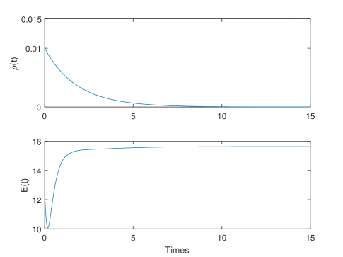
Next, let the initial epidemic probability ρ0=0.01,subscript𝜌00.01\rho_{0}=0.01, and select the appropriate initial values for nodes. And adding the controller to the first 101010 nodes with the strength di=20,i=1,,10.formulae-sequencesubscript𝑑𝑖20𝑖110d_{i}=20,i=1,\cdots,10. We set the infection rate λ=0.3>λc.𝜆0.3subscript𝜆𝑐\lambda=0.3>\lambda_{c}. Then, we can obtain the Fig. 1.

Refer to caption
Fig. 1: The epidemic probability and the synchronization errors for all nodes under the first control strategy with the infection rate λ=0.3.𝜆0.3\lambda=0.3.

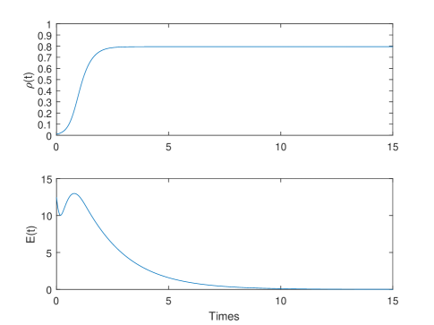
From which one can see that when the infection rate is larger than the epidemic threshold, there exists a positive stable value in the end referred by the average infected density ρ(t)𝜌𝑡\rho(t)’s (ρ(t)=i=150ρi(t)𝜌𝑡superscriptsubscript𝑖150subscript𝜌𝑖𝑡\rho(t)=\sum_{i=1}^{50}\rho_{i}(t)) curve, which means the disease will spread and will continuously exist to be the endemic disease. In this case, under the feedback control strategy, the error picture tends to zero which reflects that the network achieve behavior synchronization arouse by epidemic transmission. If we select λ=0.7,𝜆0.7\lambda=0.7, then there will be a larger stable value for ρ(t)𝜌𝑡\rho(t) as shown in Fig. 2, and the behavior synchronization resulting from disease transmission also emerge under the pinning feedback controllers.
Refer to caption
Fig. 2: The epidemic probability and the synchronization errors for all nodes under the first control strategy with the infection rate λ=0.7.𝜆0.7\lambda=0.7.

When select the infection rate less than the value 1(1+α)ρ(A)11𝛼𝜌𝐴\frac{1}{(1+\alpha)\rho(A)}, such as λ=0.06<0.0807.𝜆0.060.0807\lambda=0.06<0.0807.

Refer to caption
Fig. 3: The epidemic probability and the synchronization errors for all nodes under the first control strategy with the infection rate λ=0.06.𝜆0.06\lambda=0.06.

From the Fig. 3 one can see that the ρ(t)𝜌𝑡\rho(t) reach to zero in the end, which means the disease shall be extinct eventually. And the network will not achieve behavior synchronization with the error going to none zero result from the invalid controllers, as shown in the error curve.

Example 2.

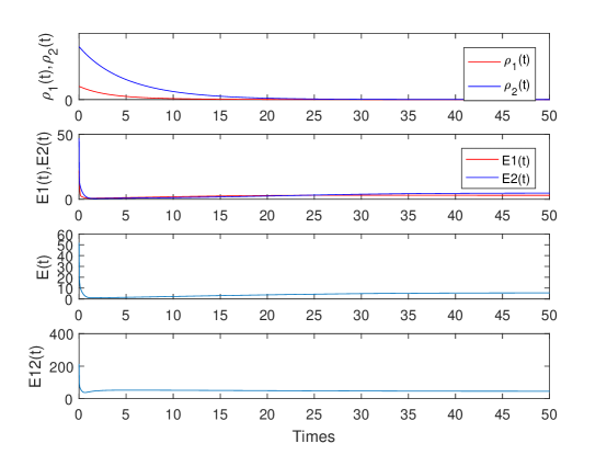
Now, we assume that the first 202020 nodes constitute the infectious individual group in the above concerned network, and the latter 303030 ones represent the susceptible group, we shall show that when the epidemic spreads, the network can reach two different behavior synchronization states for those two groups individuals via the second control strategy in this paper. In order to demonstrate this case, we introduce two types of local dynamical behaviors with the same form as Example 1, but distinct coefficient matrices as

C2=(4.5004.5),A2=(20.154.5)andC3=(1.8001.8),A3=(0.10.10.40.4).formulae-sequenceformulae-sequencesubscript𝐶24.5004.5subscript𝐴220.154.5andsubscript𝐶31.8001.8subscript𝐴30.10.10.40.4\displaystyle C_{2}=\left(\begin{array}[]{cc}-4.5&0\\ 0&-4.5\end{array}\right),A_{2}=\left(\begin{array}[]{cc}-2&-0.1\\ -5&4.5\\ \end{array}\right)~{}\text{and}~{}C_{3}=\left(\begin{array}[]{cc}-1.8&0\\ 0&-1.8\end{array}\right),A_{3}=\left(\begin{array}[]{cc}0.1&-0.1\\ -0.4&0.4\\ \end{array}\right).

Then, we can get the ζ=2.4462𝜁2.4462\zeta=2.4462 such that

(xy)T[f(x)f(y)]ζ(xy)T(xy).superscript𝑥𝑦𝑇delimited-[]𝑓𝑥𝑓𝑦𝜁superscript𝑥𝑦𝑇𝑥𝑦(x-y)^{T}[f(x)-f(y)]\leq\zeta(x-y)^{T}(x-y).

Select θ=1,𝜃1\theta=1, and we can easily get that

λmax(L11+12L12L12T)<(ζ+12),subscript𝜆subscript𝐿1112subscript𝐿12superscriptsubscript𝐿12𝑇𝜁12\displaystyle\lambda_{\max}\big{(}-L_{11}+\frac{1}{2}L_{12}L_{12}^{T}\big{)}<-\big{(}\zeta+\frac{1}{2}\big{)},
λmax(L22+12L21L21T)<(ζ+12),subscript𝜆subscript𝐿2212subscript𝐿21superscriptsubscript𝐿21𝑇𝜁12\displaystyle\lambda_{\max}\big{(}-L_{22}+\frac{1}{2}L_{21}L_{21}^{T}\big{)}<-\big{(}\zeta+\frac{1}{2}\big{)},

so the synchronization conditions in Theorem 4 are satisfied under the appropriate control strength. In this case, we select the initial infectious probabilities for two groups as ρ1(0)=0.01subscript𝜌100.01\rho_{1}(0)=0.01 and ρ2(0)=0.04,subscript𝜌200.04\rho_{2}(0)=0.04, respectively.

Then let λ=0.4>0.2422,𝜆0.40.2422\lambda=0.4>0.2422, by using the second control strategy, adding the controllers to a part of nodes in each group with the appropriate control strength, the epidemic probability reach a stable state, and the network achieve two types of behavior synchronization. In Fig. 4, one can see that the ρ1(t)subscript𝜌1𝑡\rho_{1}(t) (ρ1(t)=i=120ρi(t)subscript𝜌1𝑡superscriptsubscript𝑖120subscript𝜌𝑖𝑡\rho_{1}(t)=\sum_{i=1}^{20}\rho_{i}(t)) and ρ2(t)subscript𝜌2𝑡\rho_{2}(t) (ρ2(t)=i=130ρi(t)subscript𝜌2𝑡superscriptsubscript𝑖130subscript𝜌𝑖𝑡\rho_{2}(t)=\sum_{i=1}^{30}\rho_{i}(t)) get the positive stable values in the end. And the errors E1(t)𝐸1𝑡E1(t) and E2(t)𝐸2𝑡E2(t) in each groups and the whole errors E(t)𝐸𝑡E(t) of all nodes’ states are also tend to the zeros, while the errors E12(t)𝐸12𝑡E12(t) between two groups do not tend to zero, which indicates the main results in our paper.
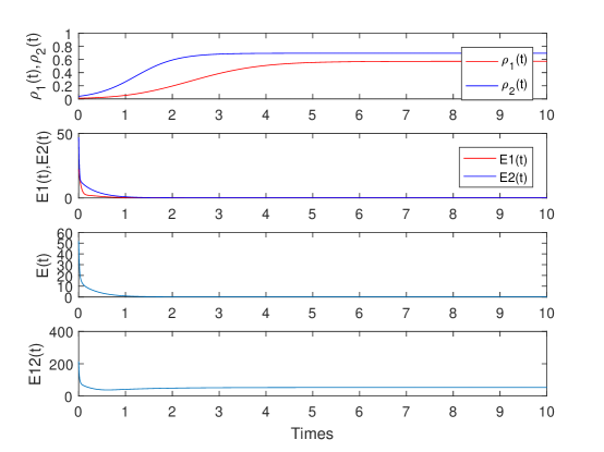
Refer to caption
Fig. 4: The ρ1(t)subscript𝜌1𝑡\rho_{1}(t), ρ2(t)subscript𝜌2𝑡\rho_{2}(t), the errors in each groups, all errors of the whole nodes’ states in the network and the errors between each groups with the infection rate λ=0.4𝜆0.4\lambda=0.4 under the second control strategy.

If we select λ=0.7,𝜆0.7\lambda=0.7, then the infectious probability for each groups will have a higher stable values, as shown in Fig. 5.
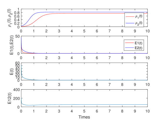
Refer to caption
Fig. 5: The ρ1(t)subscript𝜌1𝑡\rho_{1}(t), ρ2(t)subscript𝜌2𝑡\rho_{2}(t), the errors in each groups, all errors of the whole nodes’ states in the network and the errors between each groups with the infection rate λ=0.7𝜆0.7\lambda=0.7 under the second control strategy.

When the infection rate is less than the value 1(1+α)ρ(A)11𝛼𝜌𝐴\frac{1}{(1+\alpha)\rho(A)}, e.g., λ=0.07<0.0807,𝜆0.070.0807\lambda=0.07<0.0807, we can obtain Fig. 6. In which, the infectious probabilities for two groups ρ1(t)subscript𝜌1𝑡\rho_{1}(t) and ρ2(t)subscript𝜌2𝑡\rho_{2}(t) tend to zero eventually. And the errors in two groups E1(t)𝐸1𝑡E1(t) and E2(t),𝐸2𝑡E2(t), as well as the whole errors for the network do not tend to zero. Which indicates that once the infection rate is less than a certain value 1(1+α)ρ(A)11𝛼𝜌𝐴\frac{1}{(1+\alpha)\rho(A)}, the disease will be extinct in the end, and meanwhile the controllers are invalid so that none behavior synchronization.
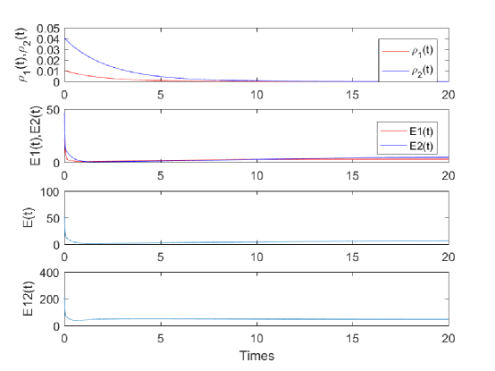
Refer to caption
Fig. 6: The ρ1(t)subscript𝜌1𝑡\rho_{1}(t), ρ2(t)subscript𝜌2𝑡\rho_{2}(t), the errors in each groups, all errors of the whole nodes’ states in the network and the errors between each groups with the infection rate λ=0.07𝜆0.07\lambda=0.07 under the second control strategy.
Remark 5.

As for the case that the infection rate is located between the value 1(1+α)ρ(A)11𝛼𝜌𝐴\frac{1}{(1+\alpha)\rho(A)} and the epidemic threshold 1(1α)ρ(A),11𝛼𝜌𝐴\frac{1}{(1-\alpha)\rho(A)}, we select two values of λ𝜆\lambda to see what changes there will be under the two control strategies. On the one hand, let λ=0.15[0.0807,0.2422].𝜆0.150.08070.2422\lambda=0.15\in[0.0807,0.2422]. Under the first control strategy, the ρ(t)𝜌𝑡\rho(t) curve and errors are shown in Fig. 7. We can see that the infectious probability tends to a stable positive value, while the network dose not get the behavior synchronization reflected by the error curve. On the other hand, let λ=0.1,𝜆0.1\lambda=0.1, and the infectious possibilities and the errors under the second control strategy are shown in Fig. 8. In that case, the infection rate tend to zero, and the errors so not. Hence, it may be more complex and varied in the case that the infection rate belongs to the interval [0.0807,0.2422],0.08070.2422[0.0807,0.2422], and some corresponding measures should be discussed according to the concrete conditions.
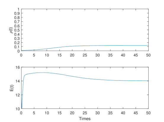
Refer to caption
Fig. 7: The epidemic probability and the synchronization errors for all nodes under the first control strategy with the infection rate λ=0.15.𝜆0.15\lambda=0.15.
Refer to caption
Fig. 8: The ρ1(t)subscript𝜌1𝑡\rho_{1}(t), ρ2(t)subscript𝜌2𝑡\rho_{2}(t), the errors in each groups, all errors of the whole nodes’ states in the network and the errors between each groups with the infection rate λ=0.1𝜆0.1\lambda=0.1 under the second control strategy.

5 Conclusions

In this paper, we investigate the epidemic controlling behavioral synchronization problem for a class of epidemic synchronous complex dynamical networks aroused from the contagions transmission, in which the quenched mean-field theory is introduced in the epidemic system. More realistically, the case of inhibition of contact behavior is concerned in the epidemic models. First, the existence of endemic equilibrium in view of the epidemic threshold and the global stability of disease-free equilibrium are discussed. Then, based on the proven technique of pinning feedback strategy, where only a part of nodes need to be controlled, and the design of two types of pinning schemes depending on nodes’ information of infection, two desired epidemic control behavior synchronization are achieved by means of the definition of behavioral synchronization. Sufficient conditions for epidemic control behavior synchronization under the contagions spreading are derived. The numerical simulations are exhibited to demonstrate the effectiveness of the main results obtained in this paper.

Acknowledgments

This work was jointly supported by the NSFC under grants 11572181 and 11331009.

References

References

  • [1] T.B. Lee, D.J. Weitzner, Creating a science of the Web, Science, 313 (5788) (2006) 769-771.
  • [2] G. Orosz, R.E. Wilson, G. Stépán, Traffic jiams: dynamics and control, Phil. Trans. Roy. Soc. A, 368 (1928) (2010) 4455-4479.
  • [3] A.L. Barabási, Z.N. Oltvai, Network biology: understanding the cell’s function organization, Nat. Rev. Gene., 5 (2) (2004) 101-113.
  • [4] A.L. Barabási, N. Gulbahce, J. Loscalzo, Network medicine: a network-based approach to hunman disease, Nat. Rev. Gene., 12 (1) (2011) 56-68.
  • [5] M. Vidal, M.E. Cusick, A.L. Barabási, Interactome networks and human disease, Cell, 144 (6) (2011) 986-995.
  • [6] J. Bascompte, Disentangling the web of life, Science, 325 (5939) (2009) 416-419.
  • [7] J.W. Wang, L.L. Rong, Cascade-based attack vulnerability on the US power grid, Safety Sci., 47 (2009) 1331-1336.
  • [8] M.H. Schweitzer, G. Fagiolo, D. Sornette, Economic networks: the net challenges, Science, 325 (5939) (2009) 422-425.
  • [9] A. Garas, P. Argyrakis, C. Rozenblat, M. Tomassini, S. Havlin, Worldwide spreading of economic crisis, New J. Phys., 12 (2) (2010) 185-188.
  • [10] P. Dodds, R. Muhamad, D. Watts, An experimental study of search in global social networks, Science, 301 (5634) 2003 827-829.
  • [11] H. Shen, Y. Zhu, L. Zhang, J.H. Park, Extended dissipative state estimation for Markov jump neural networks with unreliable links, IEEE Trans. Neural. Netw. Learn Syst., 28 (2) (2017) 346-358.
  • [12] M.E.J. Newman, Spread of epidemic disease on networks, Phys. Rev. E, 66 (1) (2002) 016128/1-11.
  • [13] H. Gao, J. Lam, G. Chen, New criteria for synchronization stability of geberal complex dynamical networks with coupling delays, Phys. Lett. A, 360 (2006) 263-273.
  • [14] J.Q. Lu, J. D. Cao, Adaptive synchronization of uncertain dynamical networks with delayed coupling, Nonlinear Dyn., 53 (1-2) (2008) 107-115.
  • [15] X. Liu, T. Chen, Cluster synchronization in community networks via intermittent pinning control, IEEE Trans. Neural Netw., 22 (2011) 1009-1020.
  • [16] K.H. Wang, X.C. Fu, K.Z. Li, Cluster synchronization in community networks with nonidentical nodes, Chaos, 19 (2009) 023106.
  • [17] S. Wang, H. Yao, The effect of control strength on lag synchrnization of nonlinear coupled complex networks, Abstr. Appl. Anal., 2012 (2012) 810364.
  • [18] W. Guo, Lag synchronization of complex networks via pinnnig control, Nonlinear Anal. RWA., 12 (2012) 2579-2585.
  • [19] M. Rosenblum, A. Pikovsky, J. Kurth, From phase to lag synchronization in coupled chaotic oscillator, Phys. Rev. Lett., 78 (1997) 4193-4196.
  • [20] H. Shen, J.H. Park, Z.G. Wu, Z. Zhang, Finite-time Hsubscript𝐻H_{\infty} synchronization for complex networks with semi-Markov jump topology, Commun. Nonlinear Sci., 24 (1-3) (2015) 40-51.
  • [21] P.R. Li, Z.J. Bao, W.J. Fan, Impulsive synchronization criteria for a class dynamical complex network with internal delay, Trans. Inst. Meas. Control, 34 (8) (2012) 927-936.
  • [22] S. Gomez, A. Arenas, Discrete-time Markov chain approach to contact-based disease spreading in complex networks, Europhys. Lett., 89 (2010) 38009.
  • [23] C.Y. Zheng, C.Y. Xia, Q.T. Guo, Interplay between SIR-based disease spreading and awareness diffusion on multiplex networks, J. Parallel Distr. Com., 115 (2018) 20-28.
  • [24] H.J. Zang, The effects of global awareness on the spreading of epidemics in multiplex networks, Phys. A, 492 (2018) 1495-1506.
  • [25] X.D. Wei, L.J. Liu, W.S. Zhou, Global stability and attractivity of a network-based SIS epidemic model with nonmonotone incidence rate, Phys. A, 469 (2017) 789-798.
  • [26] L. Xue, C. Scoglio, Network-level reproduction number and extinction threshold for vector-borne diseases, Math. Biosci. Eng., 12 (3) (2015) 565-584.
  • [27] S.P. Ansari, S.K. Agrawal, S. Das, Stability analysis of fractional-order generalized chaotic susceptible-infected-recovered epidemic model and its synchronization using active control method, Pramana J. Phys., 84 (1) (2015) 23-32.
  • [28] G. Yan, Z.Q. Fu, J. Ren, W.X. Wang, Collective synchronization induced by epidemic dynamics on complex networks with communities, Phys. Rev. E, 75 (1) (2007) 016108.
  • [29] D.G. Xu, X.Y. Xu, C.H. Yang, Spreading dynamics and synchronization behavior of periodic diseases on complex networks, Phys. A, 466 (2017) 544-551.
  • [30] Z.L. Tang, S.M. Li, Epidemic model based security analysis of firefly clock synchronization in wireless sensor networks, Internattonal J. Securtty App., 9 (6) (2015) 19-34.
  • [31] K.Z. Li, X.C. Fu, M. Small, Z.J. Ma, Adaptive mechanism between dynamical synchronization and epidemic behavior on complex networks, Chaos, 21 (3) (2011) 033111.
  • [32] K.Z. Li, Z.J. Ma, Z. Jia, M. Small, X.C. Fu, Interplay between collective behavior and spreading dynamics on complex networks, Chaos, 22 (2012) 043113.
  • [33] M.F. Sun, Y.J. Lou, J.Q. Duan, X.C. Fu, Behavioral synchronization induced by epidemic spread in complex networks, Chaos, 27 (6) (2017) 063101.
  • [34] T.P. Chen, X.W. Liu, W.L. Lu, Pinning complex networks by a single controller, IEEE Trans. Circutts-I, 54 (6) (2007) 1317-1326.
  • [35] S. Manaffam, M. K. Talebi, A. K. Jain, A. Behal, Synchronization in networks of identical systems via pinning: application to distributed secondary control of microgrids, IEEE Trans. Contr. Syst. T., 25 (6) (2017) 2227-2234.
  • [36] X.W. Liu, T.P. Chen, Synchronization of complex networks via aperiodically intermittent pinning control, IEEE Trans. Automat. Contr., 60 (12) (2015) 3316-3321.
  • [37] M.Y. Li, Z.S. Shuai, Global-stability problem for coupled systems of differential equations on networks, J. Differ. Equations, 248 (1) (2010) 1-20.
  • [38] J.Y. Wang, J.W. Feng, C. Xu, Y. Zhao, J.Q. Feng, Pinning synchronization of nonlinearly coupled complex networks with time-varying delays using m-matrix strategies, Neurocomputing, 177 (2016) 89-97.
  • [39] J.Y. Wang, J.W. Feng, C. Xu, Y. Zhao, Cluster synchronization of nonlinearly-coupled complex networks with nonidentical nodes and asymmetrical coupling matrix, Nonlinear Dyn., 67 (2) (2012) 1635-1646.
  • [40] F.Z. Zhang, Matrix Theory: Basic results and techniques, New York: Springer, (2010) pp 68.