Comparison-Based Random Forests

Abstract

Assume we are given a set of items from a general metric space, but we neither have access to the representation of the data nor to the distances between data points. Instead, suppose that we can actively choose a triplet of items $(A,B,C)$ and ask an oracle whether item $A$ is closer to item $B$ or to item $C$. In this paper, we propose a novel random forest algorithm for regression and classification that relies only on such triplet comparisons. In the theory part of this paper, we establish sufficient conditions for the consistency of such a forest. In a set of comprehensive experiments, we then demonstrate that the proposed random forest is efficient both for classification and regression. In particular, it is even competitive with other methods that have direct access to the metric representation of the data.

1 Introduction

Assume we are given a set of items from a general metric space $(\mathcal{X},\delta)$, but we neither have access to the representation of the data nor to the distances between data points. Instead, we have access to an oracle that we can actively ask a triplet comparison: given any triplet of items $(x_{i},x_{j},x_{k})$ in the metric space $\mathcal{X}$, is it true that

$$\delta(x_{i},x_{j})<\delta(x_{i},x_{k})\;\;\;\text{?}$$

Such a comparison-based framework has become popular in recent years, for example in the context of crowd-sourcing applications (Tamuz et al., 2011; Heikinheimo and Ukkonen, 2013; Ukkonen et al., 2015), and more generally, whenever humans are supposed to give feedback or when constructing an explicit distance or similarity function is difficult (Wilber et al., 2015; Zhang et al., 2015; Wah et al., 2015; Balcan et al., 2016; Kleindessner and von Luxburg, 2017).

In the present work, we consider classification and regression problems in a comparison-based setting where we are given the labels $y_{1},\ldots,y_{n}$ of unknown objects $x_{1},\ldots,x_{n}$, and we can actively query triplet comparisons between objects. An indirect way to solve such problems is to first construct an “ordinal embedding” of the data points in a (typically low-dimensional) Euclidean space that satisfies the set of triplet comparisons, and then to apply standard machine learning methods to the Euclidean data representation. However, this approach is often not satisfactory because this new representation necessarily introduces distortions in the data. Furthermore, all existing ordinal embedding methods are painfully slow, even on moderate-sized datasets (Agarwal et al., 2007; van der Maaten and Weinberger, 2012; Terada and von Luxburg, 2014). In addition, one has to estimate the embedding dimension, which is a challenging task by itself (Kleindessner and Luxburg, 2015).

As an alternative, we solve the classification/regression problems by a new random forest algorithm that requires only triplet comparisons. Standard random forests (Biau and Scornet, 2016) are one of the most popular and successful classification/regression algorithms in Euclidean spaces (Fernández-Delgado et al., 2014). However, they heavily rely on the underlying vector space structure. In our comparison-based setting we need a completely different tree building strategy. We use the recently described comparison tree (Haghiri et al., 2017) for this purpose (which in Euclidean cases would be distantly related to linear decision trees (Kane et al., 2017b; Ezra and Sharir, 2017; Kane et al., 2017a)). A comparison-based random forest (CompRF) consists of a collection of comparison trees built on the training set.

We study the proposed CompRF both from a theoretical and a practical point of view. In Section 3, we give sufficient conditions under which a slightly simplified variant of the comparison-based forest is statistically consistent. In Section 4, we apply the CompRF to various datasets. In the first set of experiments we compare our random forests to traditional CART forests on Euclidean data. In the second set of experiments, the distances between objects are known while their representation is missing. Finally, we consider a case in which only triplet comparisons are available.

2 Comparison-Based Random Forests

Figure 1: Construction of the comparison tree, illustrated in the Euclidean setting. (i) The current cell contains points with two different labels. (ii) Two pivot points with opposite labels are chosen randomly from all sample points in the current cell (circled black dots). (iii) The current cell is split according to whether points are closer to the one or the other pivot; in the Euclidean setting this corresponds to a hyperplane split. (iv) Result after recursive application of this principle with final leaf size $n_{0}=10$.

Random forests, first introduced in Breiman (2001), are one of the most popular algorithms for classification and regression in Euclidean spaces. In a comprehensive study on more than $100$ classification tasks, random forests show the best performance among many other general purpose methods (Fernández-Delgado et al., 2014). However, standard random forests heavily rely on the vector space representation of the underlying data points, which is not available in a comparison-based framework. Instead, we propose a comparison-based random forest algorithm for classification and regression tasks. The main ingredient is the comparison tree, which only uses of triplet comparisons and does not rely on Euclidean representation or distances between items.

Let us recap the CART random forest: The input consists of a labeled set $D_{n}=\{(x_{1},y_{1}),(x_{2},y_{2}),\ldots,(x_{n},y_{n})\}\subset\mathbb{R}^{d}\times\mathbb{R}$. To build an individual tree, we first draw a random subsample $D_{s}$ of $a_{n}$ points from $D_{n}$. Second, we select a random subset $Dim_{s}$ of size mtry of all possible dimensions $\{1,2,\ldots,d\}$. The tree is then built based on recursive, axis-aligned splits along a dimension randomly chosen from $Dim_{s}$. The exact splitting point along this direction is determined via the CART criterion, which also involves the labels of the subset $D_{s}$ of points (see Biau and Scornet (2016) for details). The tree is grown until each cell contains at most $n_{0}$ points—these cells then correspond to the leaf nodes of the tree. To estimate a regression function $m(x)$, each individual tree routes the query point to the appropriate leaf and outputs the average response over all points in this leaf. The random forest aggregates $M$ such trees. Let us denote the prediction of tree $i$ at point $x$ by $m_{i}(x,\Theta_{i},D_{n})$, where $\Theta_{i}$ encodes the randomness in the tree construction. Then the final forest estimation at $x$ is the average result over all trees (for classification, the average is replaced by a majority vote):

$$m_{M,n}(x;\left(\Theta_{i}\right)_{1\leq i\leq M},D_{n})=\frac{1}{M}\sum_{i=1}^{M}{m_{i}(x,\Theta_{i},D_{n})}\,.$$

The general consensus in the literature is that CART forests are surprisingly robust to parameter choices. Consequently, people use explicit rules of thumb, for example to set $\texttt{mtry}=\left\lceil d/3\right\rceil$, and $n_{0}=5$ (resp. $n_{0}=1$) for regression (resp. classification) tasks.

We now suggest to replace CART trees by comparison trees, leading to comparison-based random forests (CompRF). Comparison trees have originally been designed to find nearest neighbors by recursively splitting the search space into smaller subspaces. Inspired by the CART criterion, we propose a supervised variant of the comparison tree, which we refer to as “supervised comparison tree.”

Algorithm 1 $CompTree(S,n_{0})$:
Supervised comparison tree construction

0:  Labeled data $S$ and maximum leaf size $n_{0}$

0:  Comparison tree $T$

1:  $T.root\leftarrow S$

2:  if $|S|>n_{0}$ then

3:     Sample distinct $(x_{1},y_{1}),(x_{2},y_{2})\in S$ s.t. $y_{1}\neq y_{2}$(if all points have the same label choose randomly)

4:     $S_{1}\leftarrow\{(x,y)\in S:\delta(x,x_{1})\leq\delta(x,x_{2})\}$

5:     $T.leftpivot\leftarrow x_{1},$  $T.rightpivot\leftarrow x_{2}$

6:     $T.leftchild\leftarrow CompTree(S_{1},n_{0})$

7:     $T.rightchild\leftarrow CompTree(S\backslash S_{1},n_{0})$

8:  end if

9:  Return $T$

For classification, the supervised comparison tree construction for a labeled set $S\subset\mathcal{X}\times\{0,1\}$ is as follows (see Algorithm 1 and Figure 1): we randomly choose two pivot points $x_{1}$ and $x_{2}$ with different labels $y_{1}$ and $y_{2}$ among the points in $S$ (the case where all the points in $S$ have the same label is trivial). For every remaining point $(x,y)\in S$, we request the triplet comparison “$\delta(x,x_{1})<\delta(x,x_{2})$.” The answer to this query determines the relative position of $x$ with respect to the generalized hyperplane separating $x_{1}$ and $x_{2}$. We assign the points closer to $x_{1}$ to the first child node of $S$ and the points closer to $x_{2}$ to the other one. We now recurse the algorithm on the child nodes until less than $n_{0}$ points remain in every leaf node of the tree.

The supervised pivot selection is analogous to the CART criterion. However, instead of a costly optimization over the choice of split, it only requires to choose pivots with different labels. In Section 4.1, we empirically show that the supervised split procedure leads to a better performance than the CART forests for classification tasks.

For regression, it is not obvious how the pivot selection should depend on the output values. Here we use an unsupervised version of the forest (unsupervised CompRF): we choose the pivots $x_{1},x_{2}$ without considering $y_{1},y_{2}$.

The final comparison-based forest consists of $M$ independently constructed comparison trees. To assign a label to a query point, we traverse every tree to a leaf node, then we aggregate all the items in the leaf nodes of $M$ trees to estimate the label of the query item. For classification, the final label is the majority vote over the labels of the accumulated set (in the multiclass case we use a one vs. one approach). For regression we use the mean output value.

Algorithm 2 $CompRF(D_{n},q,M,n_{0},r)$:
CompRF prediction at query $q$

0:  Labeled dataset $D_{n}\subset\mathcal{X}\times\{0,1\}$, query $q\in\mathcal{X}$, leaf size $n_{0}$, trees $M$ and subsampling ratio $r$.

0:  $y_{q}=$ label prediction for $q$

1:  Set $C=\emptyset$ as the list of predictor items

2:  for j=1,…,M do

3:     Take a random subsample $D_{s}\subset D_{n}$, s.t., $\frac{|D_{s}|}{|D_{n}|}=r$

4:     $T_{j}\leftarrow CompTree(D_{s},n_{0})$

5:     Given $q$, traverse the tree $T_{j}$ to the leaf node $N_{j}$

6:     $C\leftarrow C\cup N_{j}$

7:  end for

8:  Return MajorityVote($\{y|(x,y)\in C\}$)

Intuitive comparison: The general understanding is that the efficiency of CART random forests is due to: (1) the randomness due to subsampling of dimensions and data points (Breiman, 1996); (2) the CART splitting criterion that exploits the label information already in the tree construction (Breiman et al., 1984). A weakness of CART splits is that they are necessarily axis-aligned, and thus not well-adapted to the geometry of the data.

In comparison trees, randomness is involved in the tree construction as well. But once a splitting direction has been determined by choosing the pivot points, the exact splitting point along this direction cannot be influenced any more, due to the lack of a vector space representation. On the other hand, the comparison tree splits are well adapted to the data geometry by construction, giving some advantage to the comparison trees.

All in all, the comparison-based forest is a promising candidate with slightly different strengths and weaknesses than CART forest. Our empirical comparison in Section 4.1 reveals that it performs surprisingly well and can even outperform CART forests in certain settings.

3 Theoretical Analysis

Despite their intensive use in practice, theoretical questions regarding the consistency of the original procedure of Breiman (2001) are still under investigation. Most of the research focuses on simplified models in which the construction of the forest does not depend on the training set at all (Biau, 2012), or only via the $x_{i}$s but not the $y_{i}$s (Biau et al., 2008; Ishwaran and Kogalur, 2010; Denil et al., 2013). Recent efforts nearly closed this gap, notably Scornet et al. (2015), where it is shown that the original algorithm is consistent in the context of additive regression models and under suitable assumptions. However, there is no previous work on the consistency of random forests constructed only with triplet comparisons.

As a first step in this direction, we investigate the consistency of individual comparison trees, which is the first building block in the study of random forests consistency. As it is common in the theoretical literature on random forests, we consider a slightly modified version of the comparison tree. We assume that the pivot points are not randomly drawn from the underlying sample but according to the true distribution of the data. In this setting, we show that, when the number of observations grows to infinity, (i) the diameter of the cells converges to zero in probability, and (ii) each cell contains an arbitrarily large number of observations. Using a result of Devroye et al. (1996), we deduce that the associated classifier is consistent. The challenging part of the proof is to obtain control over the diameter of the cells. Intuitively, as in Dasgupta and Freund (2008, Lemma 12), it suffices to show that each cut has a larger probability to decrease the diameter of the current cell than that of leaving it unchanged. To prove this in our case is very challenging since both the position and the decrease in diameter caused by the next cut depend on the geometry of the cell.

3.1 Continuous Comparison Tree

As it is the case for most theoretical results on random forests, we carry out our analysis in a Euclidean setting (however, the comparison-forest only has indirect access to the Euclidean metric via triplet queries). We assume that the input space is $\mathcal{X}=[0,1]^{d}$ with distance $\delta$ given by the Euclidean norm, that is, $\delta\left(x,y\right)=\left\lVert x-y\right\rVert$. Let $X$ be a random variable with support included in $[0,1]^{d}$. We assume that the observations $X_{1},\ldots,X_{n}\in[0,1]^{d}$ are drawn independently according to the distribution of $X$. We make the following assumptions:

Assumption 3.1.

The random variable $X\in[0,1]^{d}$ has density $f$ with respect to the Lebesgue measure on $[0,1]^{d}$. Additionally, $f$ is finite and bounded away from $0$.

For any $x,y\in\mathbb{R}^{d}$, let us define

$$\Delta(x,y)\vcentcolon=\bigl{\{}z\in\mathbb{R}^{d}\mid\delta\left(x,z\right)=\delta\left(y,z\right)\bigr{\}}\,.$$

In the Euclidean setting, $\Delta(x,y)$ is a hyperplane that separates $\mathbb{R}^{d}$ in two half-spaces. We call $H_{x}$ (resp. $H_{y}$) the open half-space containing $x$ (resp. $y$). The set $S_{1}$ in Algorithm 1 corresponds to $S\cap H_{x_{1}}$.

We can now define the continuous comparison tree.

Definition 1 (Continuous comparison tree).

A continuous comparison tree is a random infinite binary tree $T^{0}$ obtained via the following iterative construction:

• The root of $T^{0}$ is $[0,1]^{d}$;

• Assuming that level $\ell$ of $T^{0}$ has been built already, then level $\ell+1$ is built as follows: For every cell $C$ at height $\ell$, draw $X_{1},X_{2}\in C$ independently according to the distribution of $X$ restricted to $C$. The children of $C$ are defined as the closure of $C\cap H_{X_{1}}$ and $C\cap H_{X_{2}}$.

For any sequence $\left(p_{n}\right)_{n\geq 0}$, a truncated, continuous comparison tree $T^{0}(p_{n})$ consists of the first $\left\lfloor p_{n}\right\rfloor$ levels of $T^{0}$.

From a mathematical point of view, the continuous tree has a number of advantages. (i) Its construction does not depend on the responses $Y_{1},\ldots,Y_{n}$. Such a simplification is quite common because data-dependent random tree structures are notoriously difficult to analyze (Biau et al., 2008). (ii) Its construction is formally independent of the finite set of data points, but “close in spirit”: Rather than sampling the pivots among the data points in a cell, pivots are independently sampled according to the underlying distribution. Whenever a cell contains a large number of sample points, both distributions are close, but they may drift apart when the diameter of the cells go to $0$. (iii) In the continuous comparison tree, we stop splitting cells at height $\left\lfloor p_{n}\right\rfloor$, whereas in the discrete setting we stop if there is less than $n_{0}$ observations in the current cell. As a consequence, $T^{0}(p_{n})$ is a perfect binary tree: each interior node has exactly $2$ children. This is typically not the case for comparison trees.

3.2 Consistency

To each realization of $T^{0}(p_{n})$ is associated a partition of $[0,1]^{d}$ into disjoint cells $A_{1,n},A_{2,n},\ldots,A_{2^{p_{n}},n}\,.$ For any $x\in[0,1]^{d}$, let $A(x)$ be the cell of $T^{0}(p_{n})$ containing $x$. Let us assume that the responses $\left(Y_{i}\right)_{1\leq i\leq n}$ are binary labels. We consider the classifier defined by majority vote in each cell, that is,

$$g_{n}(x)\vcentcolon=\begin{cases}1\enspace\text{if}\enspace\sum_{X_{i}\in A(x)}\operatorname{\mathds{1}}_{Y_{i}=1}\geq\sum_{X_{i}\in A(x)}\operatorname{\mathds{1}}_{Y_{i}=0}\\ 0\enspace\text{otherwise.}\end{cases}$$

Define $L_{n}\vcentcolon=\operatorname{\mathbb{P}}\left(g_{n}(X)\neq Y\middle|D_{n}\right).$ Following Devroye et al. (1996), we say that the classifier $g_{n}$ is consistent if

$$\operatorname{\mathbb{E}}\left[L_{n}\right]=\operatorname{\mathbb{P}}\left(g_{n}(X)\neq Y\right)\xrightarrow[n\to+\infty]{}L^{\star}\,,$$

where $L^{\star}$ is the Bayes error probability. Our main result is the consistency of the classifier associated with the continuous comparison tree truncated to a logarithmic height.

Theorem 3.1 (Consistency of comparison-based trees).

Under Assumption 3.1, the classifier associated to the continuous, truncated tree $T^{0}(\alpha\log n)$ is consistent for any constant $0<\alpha<1/\log 2$.

In particular, since each individual tree is consistent, a random forest with base tree $T^{0}(p_{n})$ is also consistent. Theorem 3.1 is a first step towards explaining why comparison-based trees perform well without having access to the representation of the points. Also note that, even though the continuous tree is a simplified version of the discrete tree, they are quite similar and share all important characteristics. In particular, they roughly have the same depth—with high probability, the comparison tree has logarithmic depth (Haghiri et al., 2017, Theorem 1).

Table 1: Average and standard deviation of classification error for the CompRF vs. other methods. The first three rows describe datasets.

	MNIST	Gisette	UCIHAR	Isolet
Dataset Size	70000	7000	10229	6238
Variables	728	5000	561	617
Classes	10	2	5	26
KNN	2.91	3.50	12.15	8.27
CART RF	2.90 ($\pm$ 0.05)	3.04 ($\pm$ 0.26)	7.47 ($\pm$ 0.32)	5.48 ($\pm$ 0.27)
CompRF unsupervised	4.21 ($\pm$ 0.05)	3.28 ($\pm$ 0.19)	8.70 ($\pm$ 0.32)	6.65 ($\pm$ 0.14)
CompRF supervised	2.50 ($\pm$ 0.05)	2.48 ($\pm$ 0.13)	6.54 ($\pm$ 0.11)	4.43 ($\pm$ 0.26)

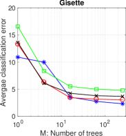
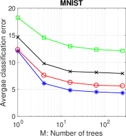
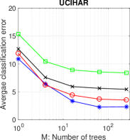
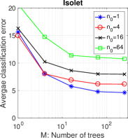
Figure 2: Average classification error of the CompRF algorithm on classification datasets. X-Axis shows the number of trees used in the forest. The title denotes the dataset and each curve corresponds to a fixed value of $n_{0}$.

3.3 Sketch of the Proof

Since the construction of $T^{0}(p_{n})$ does not depend on the labels, we can use Theorem 6.1 of Devroye et al. (1996). It gives sufficient conditions for classification rules based on space partitioning to be consistent. In particular, we have to show that the partition satisfies two properties: first, the leaf cells should be small enough, so that local changes of the distribution can be detected; second, the leaf cells should contain a sufficiently large number of points so that averaging among the labels makes sense. More precisely, we have to show that (1) $\operatorname{diam}\left(A(X)\right)\to 0$ in probability, where $\operatorname{diam}\left(A\right)\vcentcolon=\sup_{x,y\in A}\delta\left(x,y\right)$ is the diameter of $A$, and (2) $N(X)\to\infty$ in probability, where $N(X)$ is the number of sample points in the cell containing $X$. The second point is simple, because it is sufficient to show that the number of cells in the partition associated to $T^{0}(\alpha\log n)$ is $\mathrm{o}\left(n\right)$ (according to Lemma 20.1 in Devroye et al. (1996) and the remark that follows). Proving (1) is much more challenging. A sketch of the proof of (1) follows—note that the complete version of the proof of Theorem 3.1 can be found in the supplementary material.

The critical part in proving (1) is to show that, for any cell of the continuous comparison tree, the diameter of its descendants at least $k$ levels below is halved with high probability. More precisely, the following proposition shows that this probability is lower bounded by $1-\delta$, where $\delta$ is exponentially decreasing in $k$.

Proposition 3.1 (Diameter control).

Let $C$ be a cell of $T^{0}(X)$ such that $\operatorname{diam}\left(C\right)\leq D$. Then, under Assumption 3.1, the probability that there exists a descendant of $C$ which is more than $k$ levels below and yet has diameter greater than $D/2$ is at most $\delta=c\gamma^{k}$, where $c>0$ and $\gamma\in(0,1)$ are constants depending only on the dimension $d$ and the density $f$.

The proof of Proposition 3.1 amounts to showing that the probability of decreasing the diameter of any given cell is higher than the probability of keeping it unchanged—see the supplementary material.

Assuming Proposition 3.1, the rest of the proof goes as follows. Let us set $\epsilon\in(0,1)$. We are going to show that

$$\operatorname{\mathbb{P}}\left(\operatorname{diam}\left(A(X)\right)>\epsilon\right)\longrightarrow 0\quad\text{when}\quad n\to+\infty\,.$$

Let $\Gamma$ be the path in $T^{0}(\alpha\log n)$ that goes from the root to the leaf $A$ of maximum diameter. This path has length $\left\lfloor p_{n}\right\rfloor$ according to the definition of $T^{0}(\alpha\log n)$. The root, which consists of the set $[0,1]^{d}$, has diameter $\sqrt{d}$. This means that we need to divide the diameter of this cell $\pi=\left\lceil\log_{2}\sqrt{d}/\epsilon\right\rceil$ times to obtain cells with diameter smaller than $\epsilon$. Let us set $k=\left\lfloor p_{n}/\pi\right\rfloor$ and pick cells $\left(C^{(j)}\right)_{0\leq j\leq\pi}$ along $\Gamma$ such that $C^{(0)}=[0,1]^{d}$, $C^{(\pi)}=A$, and such that there are more than $k$ levels between $C^{(j)}$ and $C^{(j+1)}$. Then we can prove that $\operatorname{\mathbb{P}}\left(\operatorname{diam}\left(A\right)>\epsilon\right)$ is smaller than

$$\sum_{j=1}^{\pi}\operatorname{\mathbb{P}}\left(\operatorname{diam}\left(C^{(j)}\right)>\dfrac{\sqrt{d}}{2^{j}}\middle|\operatorname{diam}\left(C^{(j-1)}\right)\leq\frac{\sqrt{d}}{2^{j-1}}\right)\,.$$

Furthermore, according to Prop. 3.1, the quantity in the last expression is upper bounded by $\pi c\gamma^{k}$. Since $k=O\left(\log n\right)$ and $\gamma\in(0,1)$, we can conclude. ∎

Table 2: Average and standard deviation of the RMSE for the CompRF vs. CART regression forest.

	ONP	Boston	ForestFire	WhiteWine
Dataset Size	39644	506	517	4898
Variables	58	13	12	11
CART RF	1.04 ($\pm$ 0.50) $\cdot 10^{4}$	3.02 ($\pm$ 0.95)	45.32 ($\pm$ 4.89)	59.00 ($\pm$ 2.94)$\cdot 10^{-2}$
CompRF	1.05 ($\pm$ 0.50) $\cdot 10^{4}$	6.16 ($\pm$ 1.00)	45.37 ($\pm$ 4.69)	72.46 ($\pm$ 3.16) $\cdot 10^{-2}$

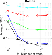
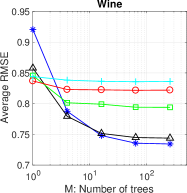
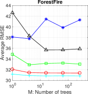
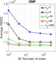
Figure 3: Average RMSE of the CompRF algorithm on regression datasets. X-Axis shows the number of trees used in the forest. The title denotes dataset and each curve corresponds to a fixed value of $n_{0}$.

4 Experiments

In this section, we first examine comparison-based forests in the Euclidean setting. Secondly, we apply the CompRF method to non-Euclidean datasets with a general metric available. Finally we run experiments in the setting where we are only given triplet comparisons.

4.1 Euclidean Setting

Here we examine the performance of CompRF on classification and regression tasks in the Euclidean setting, and compare it against CART random forests as well as the KNN classifier as a baseline. As distance function for KNN and CompRF we use the standard Euclidean distance. Since the CompRF only has access to distance comparisons, the amount of information it uses is considerably lower than the information available to the CART forest. Hence, the goal of this experiment is not to show that comparison-based random forests can perform better, but rather to find out whether the performance is still acceptable.

To emphasize the role of supervised pivot selection, we report the performance of the unsupervised CompRF algorithm in classification tasks as well. The tree structure in the unsupervised CompRF chooses the pivot points uniformly at random without considering the labels.

For the sake of simplicity, we do not perform subsampling when building the CompRF trees. We report some experiments concerning the role of subsampling in Section 3.2 of supplementary material. All other parameters of CompRF are adjusted by cross-validation.

4.1.1 Classification

We use four classification datasets. MNIST (LeCun et al., 1998) and Gisette are handwritten digit datasets. Isolet and UCIHAR are speech recognition and human activity recognition datasets respectively (Lichman, 2013). Details of the datasets are shown in the first three rows of Table 1.

Parameters of CompRF: We examine the behaviour of the CompRF with respect to the choice of the leaf size $n_{0}$ and the number of trees $M$. We perform $10$-fold cross-validation over $n_{0}\in\{1,4,16,64\}$ and $M\in\{1,4,16,64,256\}$. In Figure 2 we report the resulting cross validation error. Similar to the recommendation for CART forests (Biau and Scornet, 2016), we achieve the best performance when the leaf size is small, that is $(n_{0}=1)$. Moreover, there is no significant improvement for $M$ greater than $100$.

Comparison between CompRF, CART and KNN: Table 1 shows the average and standard deviation of classification error for $10$ independent runs of CompRF, CART forest and KNN. Training and test sets are given in the respective datasets. The parameters $n_{0}$ and $M$ of CompRF and CART, and $k$ of KNN are chosen by $10$-fold cross validation on the training set. Note that KNN is not randomized, thus there is no standard deviation to report.

Table 3: Average and standard deviation of the classification error for the CompRF in comparison with kernelSVM on graph datasets with two graph kernels: WL-subtree and WL-edge.

	MUTAG	ENZYMES	NCI1	NCI109
Train Size	188	600	4110	4127
Classes	2	6	2	2
WL-subtree kernel
Kernel SVM	17.77 ($\pm$ 7.31)	47.16 ($\pm$ 5.72)	15.96 ($\pm$ 1.56)	15.55 ($\pm$ 1.40)
KNN	14.00 ($\pm$ 8.78)	48.17 ($\pm$ 4.48)	18.13 ($\pm$ 2.27)	18.74 ($\pm$ 1.97)
CompRF unsupervised	14.44 ($\pm$ 7.94)	39.33 ($\pm$ 6.49)	17.96 ($\pm$ 1.85)	19.10 ($\pm$ 2.22)
CompRF supervised	13.89 ($\pm$ 7.97)	39.83 ($\pm$ 5.00)	17.35 ($\pm$ 1.98)	18.71 ($\pm$ 2.61)
WL-edge kernel
Kernel SVM	15.55 ($\pm$ 6.30)	53.67 ($\pm$ 6.52)	15.13 ($\pm$ 1.44)	15.38 ($\pm$ 1.69)
KNN	12.78 ($\pm$ 7.80)	51.00 ($\pm$ 4.86)	18.56 ($\pm$ 1.36)	18.30 ($\pm$ 1.82)
CompRF unsupervised	11.67 ($\pm$ 7.15)	38.50 ($\pm$ 4.19)	17.91 ($\pm$ 1.42)	19.56 ($\pm$ 1.61)
CompRF supervised	11.11 ($\pm$ 8.28)	38.17 ($\pm$ 5.35)	18.05 ($\pm$ 1.63)	18.40 ($\pm$ 2.27)

The results show that, surprisingly, CompRF can slightly outperform the CART forests for classification tasks even though it uses considerably less information. The reason might be that the CompRF splits are better adapted to the geometry of the data than the CART splits. While the CART criterion for selecting the exact splitting point can be very informative for regression (see below), for classification it seems that a simple data dependent splitting criterion as in the supervised CompRF can be as efficient. Conversely, we see that unsupervised splitting as in the unsupervised CompRF is clearly worse than supervised splitting.

4.1.2 Regression

Next we consider regression tasks on four datasets. Online news popularity (ONP) is a dataset of articles with the popularity of the article as target (Fernandes et al., 2015). Boston is a dataset of properties with the estimated value as target variable. ForestFire is a dataset meant to predict the burned area of forest fires, in the northeast region of Portugal (Cortez and Morais, 2007). WhiteWine (Wine) is a subset of wine quality dataset (Cortez et al., 2009). Details of the datasets are shown in the first two rows of Table 2.

Since the regression datasets have no separate training and test set, we assign 90% of the items to the training and the remaining 10% to the test set. In order to remove the effect of the fixed partitioning, we repeat the experiments 10 times with random training/test set assignments. Note that we use CompRF with unsupervised tree construction for regression.

Parameters of CompRF: We report the behaviour of the CompRF with respect to the parameters $n_{0}$ and $M$. We perform 10-fold cross-validation with the same range of parameters as in the previous section. Figure 3 shows the average root mean squared error (RMSE) over the 10 folds. The cross-validation is performed for 10 random training/test set assignments. The figure corresponds to the first assignment out of 10 (the behaviour for the other training/test set assignments is similar). The CompRF algorithm shows the best performance with $n_{0}=1$ for the Boston and ForestFire datasets, however larger values of $n_{0}$ lead to better performance for other datasets. We believe that the main reason for this variance is the unsupervised tree construction in the CompRF algorithm for regression.

Comparison between CompRF and CART: Table 2 shows the average and standard deviation of the RMSE for the CompRF and CART forests over the 10 runs with random training/test set assignment. For each combination of training and test sets we tuned parameters independently by cross validation. CompRF is constructed with unsupervised splitting, while the CART forests are built using a supervised criterion. We can see that on the Boston and Wine datasets, the performance of the CART forest is substantially better than the CompRF. In this case, ignoring the Euclidean representation of the data and just relying on the comparison-based trees leads to a significant decrease in performance. However the performance of our method on the other two datasets is quite the same as CART forests. We can conclude that in some cases the CART criterion can be essential for regression. However, note that if we are just given a comparison-based setting—without actual vector space representation—it is hardly possible to propose an efficient supervised criterion for splitting.

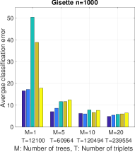
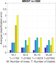
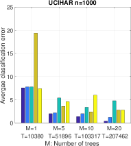
Figure 4: Average classification error of the CompRF in comparison with embedding approach on classification datasets with less than 1000 items. EmbKNN-Same (resp. EmbCART-Same) denotes the TSTE+KNN using the same triplets as CompRF, while EmbKNN-Rand (resp. EmbCART-Rand) stands for using TSTE with the same number of random triplets. X-Axis show the number of trees $(M)$ used for the CompRF and the corresponding number of triplets $(T)$ for the embedding. Each set of bars corresponds to a fixed $M$. Note that by increasing $M$, the number of triplets used by CompRF will be increased, as it appears in the X-Axis.

4.2 Metric, non-Euclidean Setting

In this set of experiments we aim to demonstrate the performance of the CompRF in general metric spaces. We choose graph-structured data for this experiment. Each data-point is a graph, and as a distance between graphs we use graph-based kernel functions. In particular, the Weisfeiler-Lehman graph kernels are a family of graph kernels that have promising results on various graph datasets (Shervashidze et al., 2011). We compute the WL-subtree and WL-edge kernels on four of the datasets reported in Shervashidze et al. (2011): MUTAG, ENZYMES, NCI1 and NCI109. In order to evaluate triplet comparisons based on the graph kernels, we first convert the kernel matrix to a distance matrix in the standard way (expressing the Gram matrix in terms of distances).

We compare supervised and unsupervised CompRF with the Kernel SVM and KNN classifier in Table 3. Note that in this setting, CART forests are not applicable as they would require an explicit vector space representation. Parameters of the Kernel SVM and $k$ of the KNN classifier are adjusted with 10-fold cross-validation on training sets.

We set the parameters of the CompRF to $n_{0}=1$ and $M=200$, as it shows acceptable performance in the Euclidean setting. We assign 90% of the items as training and the remaining 10% as the test set. The experiment is repeated 10 times with random training/test assignments. The average and standard deviation of classification error is reported in Table 3. The CompRF algorithm outperforms the kernel SVM on the MUTAG and ENZYMES datasets. However, it has slightly lower performance on the other two datasets. However, note that the kernel SVM requires a lot of background knowledge (one has to construct a kernel in the first place, which can be difficult), whereas our CompRF algorithm neither uses the explicit distance values nor requires them to satisfy the axioms of a kernel function.

4.3 Comparison-Based Setting

Now we assume that the distance metric is unknown and inaccessible directly, but we can actively ask for triplet comparisons. In this setting, the major competitors to comparison-based forests are indirect methods that first use ordinal embedding to a Euclidean space, and then classify the data in the Euclidean space. As practical active ordinal embedding methods do not really exist we settle for a batch setting in this case. After embedding, we use CART forests and the KNN classifier in the Euclidean space.

Comparing various ordinal embedding algorithms, such as GNMDS (Agarwal et al., 2007), LOE (Terada and von Luxburg, 2014) and TSTE (van der Maaten and Weinberger, 2012) shows that the TSTE in combination with a classifier consistently outperforms the others (see Section 3.1 in the supplement). Therefore, we here only report the comparison with the TSTE embedding algorithm. We choose the embedding dimension by 2-fold cross-validation in the range of $d\in\{10,20,30,40,50\}$ (embedding in more than 50 dimensions is impossible in practice due to the running time of the TSTE). We also adjust $k$ of the KNN classifier in the cross-validation process.

We design a comparison-based scenario based on Euclidean datasets. First, we let CompRF choose the desired triplets to construct the forest and classify the test points. The embedding methods are used in two different scenarios: once with exactly the same triplets as in the CompRF algorithm, and once with a completely random set of triplets of the same size as the one used by CompRF.

The size of our datasets by far exceeds the number of points that embedding algorithms, particularly TSTE, can handle. To reduce the size of the datasets, we choose the first two classes, then we subsample $1000$ items. Isolet has already less than $1000$ items in first two classes. We assign half of the dataset as training and the other half as test set. Bar plots in Figure 4 show the classification error of the CompRF in comparison with embedding methods with various numbers of trees in the forests ($M$). We set $n_{0}=1$ for the CompRF.

In each set of bars, which corresponds to a restricted comparison-based regime, CompRF outperforms embedding methods or has the same performance. Another significant advantage of CompRF in comparison with the embedding is the low computation cost. A simple demonstration is provided in Section 3.3 of the supplementary material.

5 Conclusion and Future Work

We propose comparison-based forests for classification and regression tasks. This method only requires comparisons of distances as input. From a practical point of view, it works surprisingly well in all kinds of circumstances (Euclidean spaces, metric spaces, comparison-based setting) and is much simpler and more efficient than some of its competitors such as ordinal embeddings.

We have proven consistency in a simplified setting. As future work, this analysis should be extended to more realistic situations, namely tree construction depending on the sample; forests with inconsistent trees, but the forest is still consistent; and finally the supervised splits. In addition, it would be interesting to propose a comparison-based supervised tree construction for the regression tasks.

See pages - of supplementary.pdf

References

- Agarwal et al. [2007] S. Agarwal, J. Wills, L. Cayton, G. Lanckriet, D. Kriegman, and S. Belongie. Generalized non-metric multidimensional scaling. In AISTATS, pages 11–18, 2007.
- Balcan et al. [2016] M.F. Balcan, E. Vitercik, and C. White. Learning combinatorial functions from pairwise comparisons. In COLT, pages 310–335, 2016.
- Biau [2012] G. Biau. Analysis of a random forests model. JMLR, 13(4):1063–1095, 2012.
- Biau and Scornet [2016] G. Biau and E. Scornet. A random forest guided tour. Test, 25(2):197–227, 2016.
- Biau et al. [2008] G. Biau, L. Devroye, and G. Lugosi. Consistency of random forests and other averaging classifiers. JMLR, 9(9):2015–2033, 2008.
- Breiman [1996] L. Breiman. Bagging predictors. Machine learning, 24(2):123–140, 1996.
- Breiman [2001] L. Breiman. Random forests. Machine Learning, 45(1):5–32, 2001.
- Breiman et al. [1984] L. Breiman, J. Friedman, C.J. Stone, and R.A. Olshen. Classification and regression trees. CRC press, 1984.
- Cortez and Morais [2007] P. Cortez and A.J.R. Morais. A Data Mining Approach to Predict Forest Fires using Meteorological Data. In Portuguese Conference on Artificial Intelligence, pages 512–523, 2007.
- Cortez et al. [2009] P. Cortez, A. Cerdeira, F. Almeida, T. Matos, and J. Reis. Modeling wine preferences by data mining from physicochemical properties. Decision Support Systems, 47(4):547–553, 2009.
- Dasgupta and Freund [2008] S. Dasgupta and Y. Freund. Random projection trees and low dimensional manifolds. In STOC, pages 537–546, 2008.
- Denil et al. [2013] M. Denil, D. Matheson, and N. Freitas. Consistency of online random forests. In ICML, pages 1256–1264, 2013.
- Devroye et al. [1996] L. Devroye, L. Györfi, and G. Lugosi. A probabilistic theory of pattern recognition. Springer, 1996.
- Ezra and Sharir [2017] E. Ezra and M. Sharir. A nearly quadratic bound for the decision tree complexity of k-sum. In LIPIcs-Leibniz International Proceedings in Informatics, volume 77. Schloss Dagstuhl-Leibniz-Zentrum fuer Informatik, 2017.
- Fernandes et al. [2015] K. Fernandes, P. Vinagre, and P. Cortez. A proactive intelligent decision support system for predicting the popularity of online news. In Portuguese Conference on Artificial Intelligence, pages 535–546, 2015.
- Fernández-Delgado et al. [2014] M. Fernández-Delgado, E. Cernadas, S. Barro, and D. Amorim. Do we need hundreds of classifiers to solve real world classification problems. JMLR, 15(1):3133–3181, 2014.
- Haghiri et al. [2017] S. Haghiri, D. Ghoshdastidar, and U. von Luxburg. Comparison-based nearest neighbor search. In AISTATS, pages 851–859, 2017.
- Heikinheimo and Ukkonen [2013] H. Heikinheimo and A. Ukkonen. The crowd-median algorithm. In HCOMP, 2013.
- Ishwaran and Kogalur [2010] H. Ishwaran and U. B. Kogalur. Consistency of random survival forests. Statistics & probability letters, 80(13):1056–1064, 2010.
- Kane et al. [2017a] D.M. Kane, S. Lovett, and S. Moran. Near-optimal linear decision trees for k-sum and related problems. arXiv preprint arXiv:1705.01720, 2017a.
- Kane et al. [2017b] D.M. Kane, S. Lovett, S. Moran, and J. Zhang. Active classification with comparison queries. Foundations Of Computer Science (FOCS), 2017b.
- Kleindessner and Luxburg [2015] M. Kleindessner and U. Luxburg. Dimensionality estimation without distances. In AISTATS, pages 471–479, 2015.
- Kleindessner and von Luxburg [2017] M. Kleindessner and U. von Luxburg. Kernel functions based on triplet comparisons. In NIPS, pages 6810–6820, 2017.
- LeCun et al. [1998] Y. LeCun, L. Bottou, Y. Bengio, and P. Haffner. Gradient-based learning applied to document recognition. Proceedings of the IEEE, 86(11):2278–2324, 1998.
- Lichman [2013] M. Lichman. UCI machine learning repository, 2013. Available at http://archive.ics.uci.edu/ml.
- Scornet et al. [2015] E. Scornet, G. Biau, and J.-P. Vert. Consistency of random forests. The Annals of Statistics, 43(4):1716–1741, 2015.
- Shervashidze et al. [2011] N. Shervashidze, P. Schweitzer, E.J. Leeuwen, K. Mehlhorn, and K.M. Borgwardt. Weisfeiler-lehman graph kernels. JMLR, 12:2539–2561, 2011.
- Tamuz et al. [2011] O. Tamuz, C. Liu, S. Belongie, O. Shamir, and A. Kalai. Adaptively learning the crowd kernel. In ICML, pages 673–680, 2011.
- Terada and von Luxburg [2014] Y. Terada and U. von Luxburg. Local ordinal embedding. In ICML, pages 847–855, 2014.
- Ukkonen et al. [2015] A. Ukkonen, B. Derakhshan, and H. Heikinheimo. Crowdsourced nonparametric density estimation using relative distances. In HCOMP, 2015.
- van der Maaten and Weinberger [2012] L. van der Maaten and K. Weinberger. Stochastic triplet embedding. In Machine Learning for Signal Processing (MLSP), pages 1–6, 2012. Code available at http://homepage.tudelft.nl/19j49/ste.
- Wah et al. [2015] C. Wah, S. Maji, and S. Belongie. Learning localized perceptual similarity metrics for interactive categorization. In Winter Conference on Applications of Computer Vision (WACV), pages 502–509, 2015.
- Wilber et al. [2015] M. Wilber, I.S. Kwak, D. Kriegman, and S. Belongie. Learning concept embeddings with combined human-machine expertise. In ICCV, pages 981–989, 2015.
- Zhang et al. [2015] L. Zhang, S. Maji, and R. Tomioka. Jointly learning multiple measures of similarities from triplet comparisons. arXiv preprint arXiv:1503.01521, 2015.