Evaluating and Characterizing Incremental Learning from Non-Stationary Data

Abstract

Incremental learning from non-stationary data poses special challenges to the field of machine learning. Although new algorithms have been developed for this, assessment of results and comparison of behaviors are still open problems, mainly because evaluation metrics, adapted from more traditional tasks, can be ineffective in this context. Overall, there is a lack of common testing practices. This paper thus presents a testbed for incremental non-stationary learning algorithms, based on specially designed synthetic datasets. Also, test results are reported for some well-known algorithms to show that the proposed methodology is effective at characterizing their strengths and weaknesses. It is expected that this methodology will provide a common basis for evaluating future contributions in the field.

1 Introduction

Networked computing devices are now ubiquitous. The processing capacity and size of these devices allow them to be used outside the office, allowing them to deal almost in real-time with the enormous amount of data that can be sensed from physical or virtual environments. These devices will be used more and more to process large scale continuous flows of data using machine learning techniques. In such a context, we clearly need methods for achieving Incremental Learning (IL), that is the capacity to process the data by learning methods in an incremental fashion, dealing with the changes that may occur in the environment we are sensing.

The notion of IL has been previously used in different contexts. Giraud-Carrier [1] distinguishes the concept of an Incremental Learning Task (ILT) from the concept of an Incremental Learning Algorithm (ILA). An ILT is defined as: “A learning task where the training examples used to solve it become available over time, usually one at a time.”, whereas an ILA “is incremental if, for any given training sample, it produces a sequence of hypotheses such that the current hypothesis depends only on the previous hypotheses and the current example.”. This definition implies that the task is essentially sequential, and that the algorithm implements some type of Markov process.

Some application domains that may be considered ILTs, or at least, where ILAs are usually considered well suited are:

• Learning with Concept Drift [2]. Concept drift appears when new data is not consistent with past data. This means that some unobserved aspect of reality was correlated with expected results, and varying values of that “hidden context” must force variation on learned models. Most references in this field assume a principle of batch learning, that is, complete training data is available and can be processed before the algorithm is requested to provide an answer.

• Learning from Large Datasets [3]. Defined as scenarios where a huge amount of learning data is available, which imposes constraints on the space required for representation.

• Learning from Data Streams. Defined by a continuous stream of learning data, which makes preprocessing of data unfeasible. These problems are also assumed to include the restriction that data can only be read once (one-pass learning) and usually assume non-stationarity of data A recent review of current techniques in this field can be found in [4].

• Real-time Learning. A particular case of Learning from Data Streams where hard time constraints are also imposed. The learner has to be ready to respond in a specific (usually reduced) period of time. This may also require special-purpose hardware for many applications. See [5] for some specifics in this field.

An early definition from Aha and Kibler [6] limits IL to sequential processing of examples in an instance based learning algorithm. This restrictive definition, however, provides little insight on the key issues of IL. Other more detailed definitions [7, 8, 9, 10] include a mixture of task features that incremental algorithms need to address. They vary slightly depending on the topic of the paper, for instance in [8] it is related to Learning from Large Datasets, while in [9] they are referring to Learning from Data Streams.

For the purposes of the present work, we are using the following three task features to define an ILT: Sequential Data (SD), Continuous Flow (CF), and Non-Stationary Distributions (NSD). SD simply means that data becomes available in a certain meaningful order. CF states that a never ending flow of new training data need to be learned. NSD specifies that underlying class distributions and priors may evolve over time, and thus that embedded class models should be able to adapt. An algorithm that deals with SD and CF, but not NSD, is often called online, whereas an algorithm that assumes that all training data is available before learning is called offline. An ILA is simply an algorithm capable of dealing with all three features of an ILT.

For the NSD feature, any change in class distributions can be assimilated to a concept drift. Typical class instances may thus move within the feature space, and their spread (i.e., variance of their distribution) can also evolve dynamically. But the ILT is more general than just a concept drift. Changes in class priors allow for dynamical appearance or disappearance of concepts.

Similarly, an ILA is also characterized by the following four algorithm features: Sequential Processing (SP), Online Processing (OP), Any-Time Response (ATR), and Adaptation to Change (AC). SP means that data is learned as it arrives, thus taking data ordering into account. OP implies that a complete or final data set is never expected; data should be processed in a single pass. ATR states that a prediction of the data class label must be available at any time. Finally, AC specifies that embedded class models must be able to adapt to changes in data, either stationary or non-stationary.

Other constraints arise from CF and OP: Time Invariance (TI), and Space Invariance (SI). TI means that each training sample should be processed in constant time, regardless of the amount of data encountered so-far. SI implies that internal data structures should require an approximately constant amount of memory, also independent of the amount of previously processed data.

A typical ILA will process patterns either one at a time or in chunks, creating a new model from the past model or models and new information at some intervals. In the meantime, it is able to respond with the “best guess” answer of the moment from the “current” model.

Table I summarizes how different fields of application can be classified with respect to task and algorithm features, and specifies the particular incremental learning from non-stationary data task, which is the scope of the rest of the paper.

TABLE I: Relation between areas of research in incremental learning and the various tasks, algorithms features, and constraints they consider (SD: Sequential Data, CF: Continuous Flow, NSD: Non-Stationary Distributions, SP: Sequential Processing, OP: Online Processing, ATR: Any-Time Response, AC: Adaptation to Change, TI: Time Invariance, and SI: Space Invariance).

Area	SD	CF	NSD	SP	OP	ATR	AC	TI	SI
Learning with concept drift	Yes	No	Yes	No	No	No	Yes	Weak	Weak
Learning from large datasets	No	Yes	No	No	Yes	Yes	No	Weak	Hard
Learning from data streams	Yes	Yes	Usually	Yes	Yes	Yes	Usually	Weak	Hard
Real-time learning from data streams	Yes	Yes	Usually	Yes	Yes	Yes	Usually	Hard	Hard
Learning from non-stationary data	Yes	Yes	Yes	Yes	Yes	Yes	Yes	Weak	Weak

2 IL with Non-Stationary Environments

The IL domain is vast and, as illustrated in the previous section, its scope varies according to the author. In the current work, we are restricting our review to the specific literature related to incremental learning from non-stationary data, as represented in Table I. More specifically, we are reviewing literature of related fields, analyzing the type of algorithms that are being used, the datasets used to test them, and the measurements used to evaluate and compare algorithms on those datasets.

2.1 Algorithms for Incremental Non-Stationary Learning

One of the first models that directly addresses many of the concerns specific to ILA was Adaptive Resonance Theory (ART [11]). The authors address a core issue for non-stationary systems in what they call the stability versus plasticity dilemma: learners must be able to react to significant events (plasticity) but not every event has to be learned (stability), as this can be proven to lead to unstable behavior. ART deals with the problem by being able to change between two different “learning” modes, and autonomously recognize when the algorithm should change between them.

This key issue is the concern of most of the algorithms that are specifically designed to deal with non-stationary data in an incremental manner. However, the underlying representation may vary, from classification trees to neural network or support vector approaches.

One of the first attempts at IL is IB3 [6]. In this case representation is a set of instances that are considered “relevant” and used with a nearest neighbor classification rule. Incremental learning is based on an adaptive learning and forgetting mechanism: it keeps or deletes instances based on the accuracy of the instance compared to the relative frequency of its class. As we will see later, determining which instances are relevant is a common way of “incrementalization” of algorithms whose underlying models are more complex. Nearest neighbor approaches have been studied in [12], where the authors suggest a solution based on an instance weighting approach. If a proper window size can be selected to only consider the most recent patterns, very simple lazy learning approaches can also be competitive [13].

In tree learning, an algorithm that is often referenced is CVFDT [14]. It is a decision tree classifier that is able to rapidly process new data incrementally, thus making it adequate for learning from real time data streams. It is also able to learn from non-stationary data, using a sliding window of stored patterns. The mechanism updates the current tree when new data arrives, learning the new pattern and forgetting the oldest one. When this operation invalidates parts of the current model, one or more candidate replacements are generated; when the accuracy of one of the replacements exceeds the accuracy of the current model, that part of the model is replaced by the candidate. The window size changes dynamically during the execution.

Neural network learning can usually be performed in an incremental way. For instance, in [10] an incremental online learning method for single layer Neural Networks that is able to balance learning from past and new instances, is presented. The method is based on an incremental weight adapting that was previously proven to be lossless, that is, equivalent to batch learning up to the same data. The advantage is that this network does not include an explicit change detection mechanism and does not store past models. The core of the model is a forgetting function incorporated into the objective function to be minimized by the weight adapting mechanism. Selection of the forgetting function becomes the key to efficient performance in non-stationary environments.

A field that has increasing interest in non-stationary environments is ensemble based learning. Several reviews of the specific mechanisms used in this field are available (see for instance [15]); one of the basic reasons to use ensembles is that the incremental and adaptive part of the algorithm can be achieved independently of the nature of the base classifier used.

One of the first attempts on this subject can be found in [8]. In this case, classifiers are built based on small chunks of training data; when the ensemble is complete, new classifiers can replace old ones based on the accuracy increase over the new chunks of data. This allows the complete ensemble to self-adapt to changing data.

A typical mechanism for ensemble learning is dynamic combination. For instance, this is used in Learn++ [16] to learn incrementally in the context of non-stationary data. The ensemble dynamically combines classifiers based on weights that depend on the success rate of each classifier for the current dataset. So this weight allocation is the part of the algorithm that is incremental and able to adapt to non-stationary data. In recent versions of this ensemble approach, such as Learn++.NSE [7], ensembles that had good accuracy in the past are not deleted, so they can become active in the future. In this way, if the nature of the change is cyclical, the algorithm will have an advantage when past conditions reappear. Another aspect of incremental learning is considered in [17], that has a better behavior in situations where new classes appear in data.

Also new data can be used to update the underlying classifiers, using mechanisms derived from the bagging or boosting batch learning algorithms. Online bagging or boosting were proposed by Oza [18]; and variants have been proposed that take into account non-stationary data, such as ONSBoost [19]. An analysis of several versions of online bagging or boosting is performed in  [20].

2.2 Incrementalization of Algorithms

Renewed interest on incremental algorithms has led to a significant trend in research that tries to adapt existing non-incremental algorithms to an incremental behavior.

This incrementalization approach can be conducted in several ways:

• Adapt the learning mechanism itself so it becomes purely incremental. For instance, weights on a Neural Network are adapted every time a new pattern is available to the system.

• Use an instance windows or instance weighting mechanism but make no modifications to the algorithm itself; recalculate model at fixed intervals using these windows or weights to decide which data is used for training the new model.

• Use all or part of the data to create an initial model; monitor changes in data (using a detection function) and rebuild the model whenever deemed necessary based on new data.

Several studies have adapted non-incremental classification methods in one of the above ways:

• Basic lazy learning algorithms, such as K-Nearest Neighbor can be transformed into robust non-stationary classifiers provided they perform classification using only a certain number of the most recent patterns received for training (window size, $wsize$). If this parameter is well suited for a given problem, this approach can outperform some popular NSL methods [13].

• Evolutionary algorithms may adapt to change if a change detection mechanism is implemented and used to vary their parameters. For instance in [21] an Adaptive Genetic Programming classifier is used for non-stationary data. In this case, data is divided in separate windows, either overlapping or non-overlapping. For every window change, a number of iterations is required in order to allow the algorithm to converge to a solution.

• Other classifiers based on an incremental concept use an incremental version of Growing Neural Gas (GNG) as a way of positioning prototypes. GNG is a clustering method that aims to learn a topology. Its behavior is unsupervised, but in Supervised Neural Gas [22], GNG units may be used as centers for a Radial Basis Function Neural Network to be applied to classification. In [23] it was shown how GNG can adapt to slow changes due to its forgetting mechanism, so this feature may be used to implement adaptation to change.

• Incremental algorithms have been proposed for vector quantization methods, including Incremental Learning Vector Quantization [24], that is claimed to work in non-stationary environments.

• Online Support Vector Machine (OSVM) is usually oriented to provide efficient SVM implementations able to deal with large datasets. Depending on implementation, algorithms are able to perform sequential and online processing, and deliver anytime response, but the SVM model is not able to adapt to change. In [25] an exact version of support vector learning is documented, that provides optimal adjustment of the SVM support vectors given a new sample. In [26] some implementation issues are studied in order to provide an efficient support vector learning algorithm.

• Stochastic Gradient Descent (SGD) techniques have been proven in [27] to be successful options for online classification of large datasets using SVMs. The accuracy loss due to its approximate nature (compared to exact optimization techniques) is easily balanced by its computational effectiveness. The method can be incremental as SGD does not remember which examples were used to adjust the classifier in previous iterations. SGD update functions are provided for several classification and regression algorithms, including Adaline, Perceptron, and SVMs.

2.3 Algorithms Dealing with Concept Drift

The field of Concept Drift (CD) explicitly deals with non-stationary data, while the incremental nature of learning is not required. Most work is related to algorithms that work on complete training datasets in batch mode. However, there is a trend that is moving towards considering how mechanisms might work on online scenarios. A comprehensive review of the field can be found in [28].

A learning task with CD can be characterized in terms of two orthogonal dimensions: drift frequency [29] and drift extent [30]. The authors work with bounding those dimensions in order to ensure a certain degree of learning ability from a non-stationary flow of data.

Widmer and Kubat [31] introduce several important topics in this area and propose some techniques to deal with them. This article provides a set of algorithms, called the FLORA family, each version improving a specific aspect of the problem. The basic mechanisms these algorithms use are an adaptive window of trusted data and a repository of hypotheses. The algorithm monitors the appearance of concept drifts by tracking changes in accuracy.

A family of algorithms based on Info-Fuzzy networks is formed by OLIN, IOLIN and Enhanced and Multiple Model IOLIN [32, 33, 34]. The first algorithm uses a regenerative approach, constructing new models for each block of data (defined by a sliding window). The second adopts an incremental approach whenever no major concept drift is detected between windows. The third work introduces further enhancements and a way of recovering old models that become reusable.

In [35], the authors carry out an extensive treatment of concept drift using non-incremental classifiers (SVM), but adopting a weighting schema for patterns used for learning. Several cases are examined, ranging from sudden change to slow drift. The authors claim that incremental versions of SVM were not of interest as they are not designed for non-stationary data.

2.4 Evaluation Metrics

Evaluating the performance of ILA presents specific problems and must take into account aspects not present in conventional evaluation of learning.

Early papers such as [6] already described measures of performance that are aimed to address each of the significant characteristics of so-called “incremental algorithms”. In that work, measures that should be taken into account when evaluating the success of a ILA are:

1. Generality: This is the kind of concept which can be described by the representation mechanism and is learnable by the algorithm.

2. Accuracy: This is the classification accuracy, either in terms of averaged success or error rate.

3. Learning Rate: This is the speed at which classification accuracy increases during training. It is a more useful indicator of the performance of the learning algorithm than the accuracy for finite-sized training sets.

4. Incorporation Costs: These are the costs incurred while updating the concept descriptions with a single training instance. They include classification costs.

5. Storage Requirement: This is the size of the concept description (for instance for instance-based algorithms, it is defined as the number of saved instances used for classification decisions).

Measures of accuracy and learning rate can be extended for non-stationary data scenarios. However, accuracy has to be measured in a specific way due to the continuous nature of learning, because traditional accuracy measures assume that: a) the dataset is finite; b) the concepts represented by learning do not change. We shall use learning rate to describe how the algorithm reacts to changes in data.

The continuous nature of input data means that common ways of estimating accuracy of learning cannot be used. This applies to train-and-test, cross-validation, or leave-one-out methods, which are common practice in batch learning, where a representative test set can be separated from training data at the beginning of the learning phase and used only for validation of the generated model after training.

Almost every published paper that deals with non-stationary data evaluates its performance by graphically comparing accuracy plots, either using an accumulated accuracy or displaying average accuracy over a sliding window of fixed size, to be able to account for transient states where algorithms are adapting to changes.

Two different methods have been used to evaluate accuracy of incremental algorithms [9]: using a separate holdout set of patterns for testing; or using Predictive Sequential (Prequential) evaluation. The latter has the advantage that no explicit test set has to be defined and extracted from data. Discussion on how prequential error relates to holdout error can be found in [9], and analysis of prequential statistics is available in [36].

Average Prequential Error ($AE_{preq}$) is the average value of the classification error when patterns are presented to the current model and before the model can learn from them. After evaluation, the pattern(s) can be used to update (train) the model. For this reason this evaluation method is also referred to as the Interleaved Test-then-Train method.

Most papers do not take into consideration an explicit measure of how algorithms perform in terms of Learning Rate, Incorporation Costs or Storage Requirements. Sometimes temporal plots of the prequential error are used, where the time axis corresponds to the number of patterns used for training. This measure can be labelled as $AE_{preq}(n)$, where $n$ is the time, or pattern number, up to which the error is averaged.

The value of $AE_{preq}(n)$ can be calculated as:

$$AE_{preq}(n)=\frac{1}{n}\sum_{i=1}^{n}L(p_{i},o_{i}),$$ (1)

where $p_{i}$ is the prediction for pattern $i$ and $o_{i}$ the observed value for $i$, while $n$ is the number of patterns over which the error is measured, and $L$ a loss function. The loss function can be defined as the 0-1 loss for achieving conventional classification:

$$L(p_{i},o_{i})=\left\{\begin{array}[]{ll}0,&\mbox{if }p_{i}=o_{i}\\ 1,&\mbox{otherwise}\end{array}\right..$$ (2)

For finite-size datasets, algorithms are compared using this value over the whole process ($AE_{preq}$), that is, we use Eq. 1 for a value of $n$ equal to the number of patterns in the dataset.

It is also useful to observe the actual behavior of error at every stage, in order to remove the effect of the accumulation of the past errors. Thus, a third measure is used, $AE^{w}_{preq}(n)$, that is, the average prequential error calculated over a sliding window of $w$ (window size) patterns:

$$AE_{preq}^{w}(n)=\frac{1}{w}\sum_{i=n-w}^{n}L(p_{i},o_{i}).$$ (3)

Additional topics are being introduced in this field. One of these issues is described in [37]. When dealing with imbalanced class distributions, algorithms may fail to take into account patterns with lower frequencies. We consider that this aspect is also interesting in a non-stationary environment, as class frequencies are not available from the outset and determining whether the set is balanced or imbalanced cannot be decided in advance.

In [38] the authors introduce a novel measure for assessment of IL algorithms, called Recovery Analysis. This metric describes behavior of the algorithms in the moment of change between two stationary states, by measuring the maximum decrease in performance and the recovery time required by each algorithm.

Finally in [39], the authors realize that most scenarios depend on the assumption of temporal independence of data and propose a procedure and a metric that can be used when that assumption is not true.

2.5 Datasets

Several artificial and real-world datasets have been used to test algorithms with non-stationary data. Most of these datasets were produced from the Concept Drift field. Several datasets are referenced in [20], with some of these sets being presented in Table II.

TABLE II: Relation of datasets frequently used in literature for learning from non-stationary data. A: Artificial Dataset, R: Real dataset, At: number of attributes, Cl: number of classes

Dataset	Reference	A/R	At	Cl
SEA concepts generator	[8]	A	3	2
STAGGER concepts	[40]	A	3	2
LED Generator	[41]	A	24	2
Rotating Hyperplane	[14]	A	V	2
Rotating Gaussian	[42]	A	2	2
Electricity dataset	[43]	R	7	2
Traffic data streams	[34]	R	12	7
Brain-computer interface	[44]	R	5	2
Mountain Fire scenario	[42]	R	3	2

Unfortunately, these datasets are being used without much information concerning the type of problems they bring to the learning algorithms. It would be desirable to have some information on the specific features that these datasets are expected to test in algorithms. Also, there is a lack of reference values to which actual performance on these datasets can be evaluated, and most papers basically compare the proposed algorithm in some of these datasets without further information on how the selected dataset was chosen.

For artificial datasets, another problem arises when instead of the datasets themselves, only dataset generation algorithms are described, based on some parameters and/or random initialization. Parameters may include dimensionality, size of concept drift, etc. Also, some authors use random radial basis functions (Random RBF generators) [20]. In those cases it is in general impossible to determine whether actual data sources were close, distant, separable or superimposed. Some authors describe their artificial datasets with more detail. For instance, in [15] several artificial datasets are proposed. For each dataset, the type of change is described, and for each dataset a Severity measure indicates the percentage of the input space whose class changes after the drift is complete.

3 IL Evaluation Methodology

In this work we propose an evaluation methodology for testing the capabilities of any algorithm in dealing with incremental learning tasks. The aim of this methodology is to formalize a test bench that can be used to evaluate incremental algorithms able to learn from non-stationary data.

In this way we design a set of evaluation tests, corresponding to features that should be considered in the evaluation of any incremental learning algorithm. Each evaluation test is composed of a dataset, its optimal Bayes error (that is, a minimal error bound for the dataset) and the description of the dynamics of the data transformation, including changes in class distributions and class priors.

3.1 Algorithms

Before presenting the various test benchmarks, which is the core contribution of this paper, we want to introduce the various learning methods that will be tested against these benchmarks, These methods will be tested to assert that the proposed benchmarks are properly measuring the specific property that we want to assess.

This selection of reference algorithms is by no means exhaustive over all possible incremental algorithms in the literature. We selected a varied set of algorithms whose behaviors, strengths and weaknesses are well known and understood. Indeed, by using algorithms of different types, we hope to see how different mechanisms are responsible for good or bad results in each of the defined objectives.

We have used the Massive Online Analysis (MOA) [45] software environment to provide the algorithms and run the experiments. Among the algorithms it provides, we have selected the following:

Naive Nayes (NB) constructs a static model from which we can assess how classifiers designed for stationary data degrade in the non-stationary case. This version of Naive Bayes calculates its model incrementally.

Stochastic Gradient Descent (SGD) has been used to train classifiers for large-scale problems (e.g.  [27]). We use it for NSL because, under certain assumptions related to the number and type of classifier, it is able to quickly adapt to non-stationary data. The version we selected uses a two-class SVM with linear kernel.

Dynamic Weighted Majority (DWM) [46] is an ensemble method that is able to classify non-stationary data using a dynamic weight assignment to base classifiers that depends on their current accuracy. Classifiers are created or pruned dynamically. We used a Naive Bayes base learner for DWM.

OZABAG-ADWIN [20] is an online bagging method that is adapted to concept drift by using a self-adapting window of patterns for training. Window size is changed depending on a decision function called ADWIN. This type of change detector monitors a random variable and decides if a change has taken place depending on the result of a statistical test performed on the value of the variable measured over two different sets of data: past data and current data. For instance, ADWIN detects change in the mean values of the false positive rate of the classifier. If both values of the averages false positive rate differ significantly given a certain confidence value, the window size is reduced by removing old data. We used a ensemble of $10$ base classifiers, each one learns a Hoeffding tree structure using CVFDT [14].

Although NN classification may seem elementary, we use this approach to assess the success of time-based forgetfulness. By using a fixed-size sliding window, the algorithm will use only recent data for classification. Obviously the selection of the proper window size becomes the problem in that case. We therefore investigate three window sizes: NN¹⁰⁰, NN¹⁵⁰⁰, and NN⁶⁰⁰⁰. The smaller window (100) tends to favor adaptation to change, while the larger one (6000) tends to increase accuracy.

We must remark here that it is not our intention, per se, to test the accuracy and performance of these methods. The methods were not chosen for their particular performance or popularity, but rather to set up an experimental environment to validate the efficacy of our methodology for the comparison of different incremental learning methods.

3.2 Properties of interest

The key point, when designing a testing methodology, is to determine exactly what needs to be measured. For instance, we might wish to evaluate “plasticity”, but this type of concept is too vague to be practical. Another approach would be to enumerate all possible data transformations. Assuming Gaussian distributions, this means moving centers and changing variances in different directions, using different dynamics. Obviously, we need to restrict ourselves to a subset of possibilities.

In this context, the following properties were selected in order to guide the creation of data models that are apt at evaluating the adaptive capabilities of incremental learning algorithms:

1. Contradiction in the presence of global change; contradiction refers to non stationarity that causes new knowledge to disagree with older knowledge; adaptability to this requires some form of forgetfulness; global change refers to distributions that simultaneously all undergo similar transformations.

2. Contradiction in the presence of local change; in contrast to global change, local change refers to different transformations applied to different distributions.

3. Long-term memory; refers to past knowledge that has not been used for a while, but then becomes useful again; adaptability to this assumes that forgetting mechanisms are not exclusively time-based.

4. Change in distribution frequency; refers to priors that change over time.

5. Appearance of new concepts; refers to new distributions that are, at some point in time, added to existing mixtures, or that create whole new classes.

6. Speed of change; refers to the scale of non-stationarity, that is slow vs fast changes.

7. Effect of dimensionality; refers to the input feature space dimensionality.

8. Complex non-stationary changes; refers to combinations of other relevant properties.

3.3 Data Modeling and Generation

In the following, we model data using a mixture of mixtures. Let $C_{i}^{t}$ denote the $i^{th}$ class at time $t$, $i=1,\ldots,K^{t}$, of a non-stationary $K^{t}$-class problem. Each class is modeled by a mixture of $k_{i}^{t}$ distributions $\{{\cal G}_{i,1}^{t},\ldots,{\cal G}_{i,k_{i}^{t}}^{t}\}$, where exponent $t$ stresses the time dependence of the distributions. Then, the density function $p(\mathbf{x},t)$ represents the probability of observing vector $\mathbf{x}$ at time $t$:

$$p(\mathbf{x},t)=\sum_{i=1}^{K^{t}}\sum_{j=1}^{k_{i}^{t}}P({\cal G}_{i,j}^{t})\,p(\mathbf{x}\,|\,{\cal G}_{i,j}^{t}),$$ (4)

where $P({\cal G}_{i,j}^{t})$ is the a priori probability of the $j^{th}$ distribution of $C_{i}^{t}$ and $p(\mathbf{x}\,|\,{\cal G}_{i,j}^{t})$ the density function of ${\cal G}_{i,j}^{t}$. With such a model, the probability that $\mathbf{x}$ belongs to $C_{i}^{t}$ is expressed by:

$$P(C_{i}^{t}\,|\,\mathbf{x},t)=\frac{\sum_{j=1}^{k_{i}^{t}}P({\cal G}_{i,j}^{t})\,p(\mathbf{x}\,|\,{\cal G}_{i,j}^{t})}{p(\mathbf{x},t)}.$$ (5)

This equation defines the ground truth. The optimal Bayesian classifier is obtained by selecting, for a pattern $\mathbf{x}$, the class $i$ that maximices $P(C_{i}^{t}\,|\,\mathbf{x},t)$.

If we arbitrarily set $p(\mathbf{x}\,|\,{\cal G}_{i,j}^{t})\sim{\cal N}(\bm{\mu}_{i,j}^{t},\bm{\Sigma}_{i,j}^{t})$, a multidimensional Gaussian distribution with center $\bm{\mu}_{i,j}^{t}$ and covariance matrix $\bm{\Sigma}_{i,j}^{t}$, the data model becomes a mixture of Gaussian mixtures.

To generate data using this model, at each discrete time step $t$, we first randomly select distribution ${\cal G}_{s}^{t}$ with probability:

$$P_{s}=\frac{P({\cal G}_{s}^{t})}{\sum_{i=1}^{K^{t}}\sum_{j=1}^{k_{i}^{t}}P({\cal G}_{i,j}^{t})},$$ (6)

using a proportional random selection, and then generate $\mathbf{x}$ using $p(\mathbf{x}\,|\,{\cal G}_{s}^{t})$.

3.4 Model Description

Models are described by a set of named classes (typically “A”, “B”, “C”, etc.), composed of a weight parameter plus a mixture of Gaussian distributions. Distributions are specified by a start time index, a weight parameter, an initial position (center), an initial covariance matrix, and a sequence of cascading transforms. Each transform is associated with a duration parameter, during which a shape preserving (similarity) transformation is applied linearly; the transform is defined by rotation angles, scale factor, and translation.

The start index of a distribution determines at which time it begins to exist. Before that index, it is not part of the class mixture. The class itself starts to exist at the beginning of its first distribution. The duration of a distribution is equal to the sum of the durations of its cascade of transforms. To exist, a distribution must thus define at least one transform with a non null duration. To set a stationary distribution, an identity transform should be specified (the default), that is a transform with unit scale, null rotation, and null translation.

The rotation and scale parameters of a transform are applied to the covariance matrix of its Gaussian distribution, while the translation parameters are applied to its center position. The transforms are sequential and cumulative, with each transform defining a separate phase of non-stationarity. The distribution at the beginning of a new transform is equal to the distribution at the end of the previous transform. A transform is applied gradually, in a linear fashion, during its full duration. For an instantaneous transformation, the duration parameter should be set to zero.

The weights of classes and distributions are used to determine the distribution priors that enable data generation. Let $w_{i}$ denote the weight associated with class $C_{i}$, and $w_{i,j}$ the weight of distribution ${\cal G}_{i,j}$. Then, prior $P({\cal G}_{s,v}^{t})$ of some active distribution ${\cal G}_{s,v}^{t}$ at time $t$ is computed by:

$$P({\cal G}_{s,v}^{t})=\frac{w_{s}w_{s,v}}{\sum_{i=1}^{K^{t}}w_{i}\sum_{j=1}^{k_{i}^{t}}w_{i,j}},$$ (7)

where $K^{t}$ is the number of active classes at time $t$, and $k_{i}^{t}$ the number of active distributions within the mixture of class $C_{i}^{t}$.

4 Datasets and results

In this section, we go through all of the properties that were presented in Section 3.2 and describe the corresponding datasets that are proposed to test these properties. We then apply these datasets to all of the algorithms presented in Section 3.1 and report results.

TABLE III: Results for all datasets, values are final $AE_{preq}$ in %.

Problem	Opt.	NB	SGD	DWM	OZAB	NN100	NN1500	NN6000
NSGT	2.95	25.27	7.68	4.21	4.20	4.83	6.77	10.97
NSGT-F	2.91	41.73	14.14	6.90	4.39	4.77	11.79	12.04
NSGR	0.00	49.61	0.04	0.90	0.54	0.02	0.02	36.95
NSLC	4.05	6.44	4.25	4.91	4.72	6.19	6.12	7.77
NSGT-I	2.93	25.05	8.02	5.85	4.48	4.80	9.58	10.28
NSPC	5.76	5.94	6.77	6.24	6.16	9.00	8.73	8.90
NSPC-A	5.37	6.09	5.89	6.09	5.98	8.45	8.28	8.82
NSGT-5D	5.74	25.43	9.35	7.34	7.63	12.18	11.16	11.88
NSCX	4.18	14.28	12.94	6.90	6.08	6.47	8.62	10.19

In Table IV we summarize the parameters used for each of the datasets. All datasets are two-dimensional and have $10000$ patterns. For each distribution in a dataset, a sequence of transitions describe the changes applied to the distribution parameters. Distributions and transitions are also described graphically in Fig 1.

TABLE IV: Summary of dataset parameters. Transform types: rmoveto$(r_{x},r_{y})$, relative translation of $r_{x},r_{y}$ units; wchangeto$(w)$, linear change from current weight to $w$; scale$(s)$, linear change in variance until its value is multiplied by s; rotate$(g)$, rotation of $g$ degrees

dataset	dims	size	initial distributions parameters					phases of transformation
			class	weight	center	stddev	rotation	period	transform type
NSGT	2	10001	A	1.0	$(0.0,0.0)$	$(2.5,1.0)$	$45^{\circ}$	0-9999	rmoveto$(10,10)$
			B		$(5.0,0.0)$		$-45^{\circ}$
NSGT-F	Same as NSGT							0-9999	rmoveto$(30,30)$
NSGR	2	10001	A	1.0	$(10.0,0.0)$	($2.0,5.0$)	$45^{\circ}$	0-9999	rotate once around origin
			B		$(-10.0,0.0)$
NSLC	2	10001	A	1.0	$(-2.0,2.0)$	$(2.5,1.0)$	$45^{\circ}$	0-9999	rmoveto$(0.0,-4.0)$
			B		$(2.0,-2.0)$		$-45^{\circ}$		rmoveto$(0.0,4.0)$
NSGT-I	2	10001	A	1.0	$(0.0,0.0)$	$(2.5,1.0)$	$45^{\circ}$	0-4999	rmoveto$(10,10)$
								5000	rmoveto$(-10,-10)$
								5001-10000	rmoveto$(10,10)$
			B		$(5.0,0.0)$		$-45^{\circ}$	0-4999	rmoveto$(10,10)$
								5000	rmoveto$(-10,-10)$
								5001-10000	rmoveto$(10,10)$
NSPC	2	10001	A1	$0.05$	$(-2.0,0.0)$	$(2.5,1.0)$	$45^{\circ}$	500-9499	wchangeto$(0.45)$
			A2	$0.45$	$(2.0,0.0)$		$-45^{\circ}$		wchangeto$(0.05)$
			B	$0.5$	$(0.0,3.5)$	$(1.0,1.0)$	$0^{\circ}$
NSPC-A	2	10001	A1	0.0	Same as NSPC			5000	wchangeto$(0.5)$
			A2	0.5					wchangeto$(0.0)$
			B	0.5	Same as NSPC
NSGT-5D	5	10001	A	0.5	$(0.0,0.0,0.0,0.0,0.0)$	$(1.0,1.0,1.0,$	$0^{\circ}$	0-9999	rmoveto$(6.3,6.3,6.3,6.3,6.3)$
			B		$(3.15,0.0,0.0,0.0,0.0)$	$1.0,1.0)$
NSCX	2	10001	A1	$0.65$	$(0.0,0.0)$	$(2.5,1.0)$	$30^{\circ}$	0-4999	rmoveto$(5.0,5.0)$, rotate$(90^{\circ})$, scale$(2)$
								5000-9999	rmoveto$(5.0,5.0)$, wchangeto$(1.00)$
			A2	$0.35$	$(0.0,-4.0)$	$(0.6,2.0)$	$0^{\circ}$
			B	$0.0$	$(-2.0,3.0)$	$(1.5,0.5)$	$0^{\circ}$	0-499	wchangeto$(0.2)$
				$0.2$				500-1999	rmoveto$(3.0,-4.0)$,rotate$(30^{\circ})$, wchangeto$(0.5)$
				$0.5$				2000-4499	rmoveto$(4.0,-1.0)$,rotate$(30^{\circ})$, wchangeto$(0.8)$
				$0.8$				4500-9999	rmoveto$(6.0,5.0)$,rotate$(30^{\circ})$, wchangeto$(1.0)$

We have generated ten versions of each of the datasets, using different random seeds for sampling. Hereafter we report average results for these ten runs, and graphics are also generated using the average result for each data point. This allows a reduced variance in the average results and produces smoother graphics. Whenever results are shown, boldface indicates the best algorithm. This comparison does not take into account the Bayes Optimal classifier which is listed in the first column. All algorithms whose average result is not significantly different from the best, with a significance value of $\alpha=0.05$, are also in boldface. This comparison was made using pairwise Wilcoxon tests.

Results of these experiments are summarized in Table III, where we show the value of the Average Prequential Error ($AE_{preq}$, see Eq. 1) at the end of the datasets.

4.1 Contradiction in the Presence of Global Change

The first two datasets seek to evaluate the adaptability to global contradiction, that is, the ability of algorithms to modify their internal model in order to globally follow moving distributions that are linked together in some way. In these datasets, contradictions are introduced gradually, by translating both distribution centers in order to maintain their relative positions, so that the samples of one distribution gradually occupy the position of previous samples of the other.

NSGT (for non-stationary global translation) starts with two overlapping distributions that drift linearly in a fixed direction, preserving their relative positions and orientations, see Fig. 1a. NSGR simulates the rotation of the two distribution centers around a mid-point, see Fig. 1b. Contradictions will begin to appear when the angle of rotation approaches 180 degrees and will continue for an additional 180 degrees.

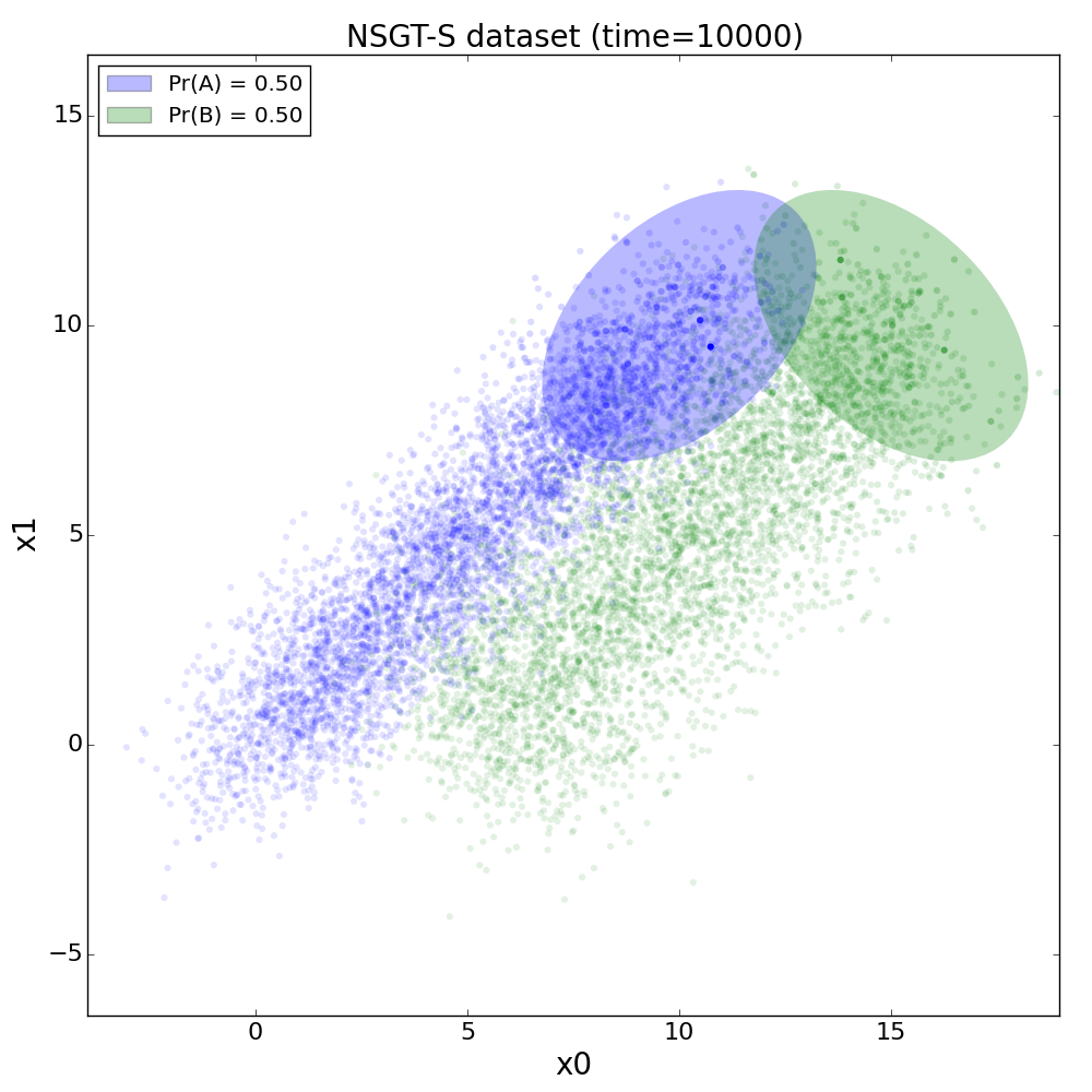
(a) NSGT, NSGT-I and NSGT-F

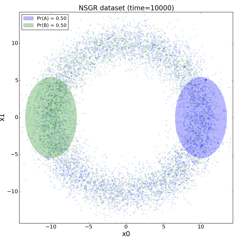
(b) NSGR

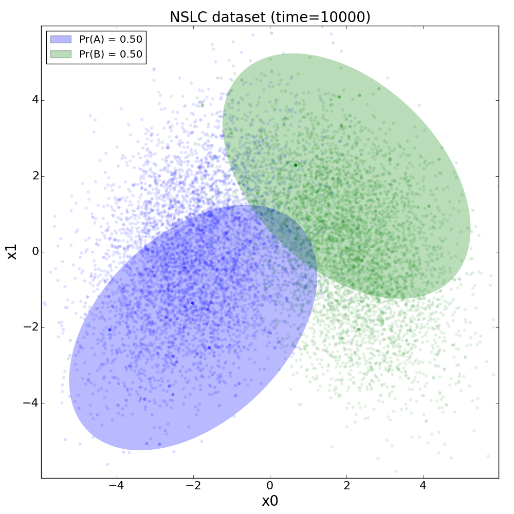
(c) NSLC

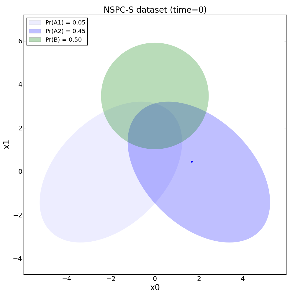
(d) NSPC: Start

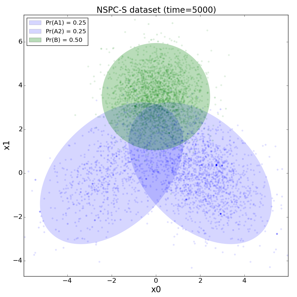
(e) NSPC: Pattern 5000

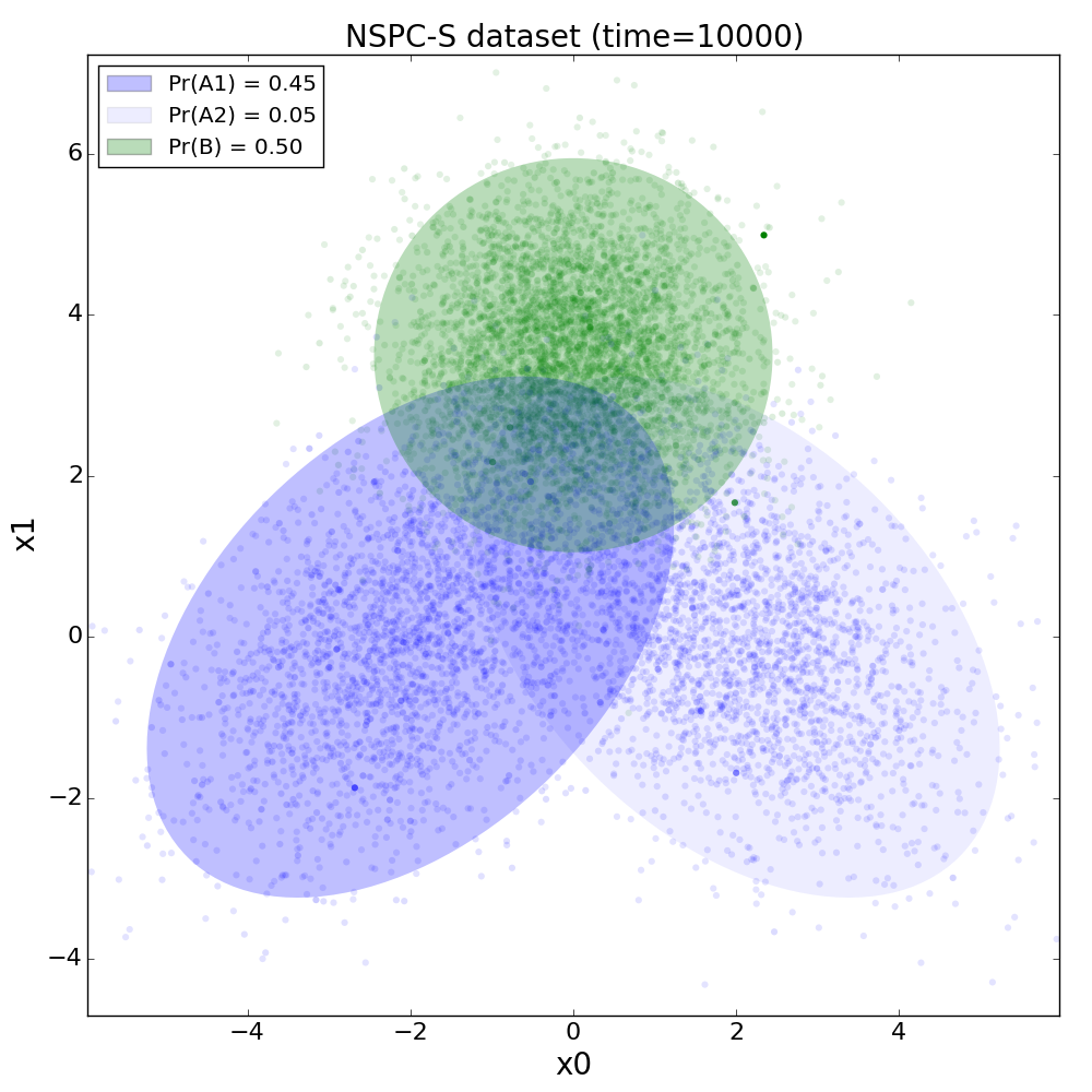
(f) NSPC: Pattern 10000

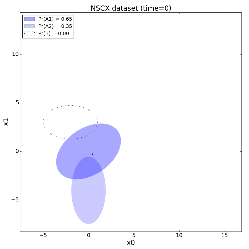
(g) NSCX: Start

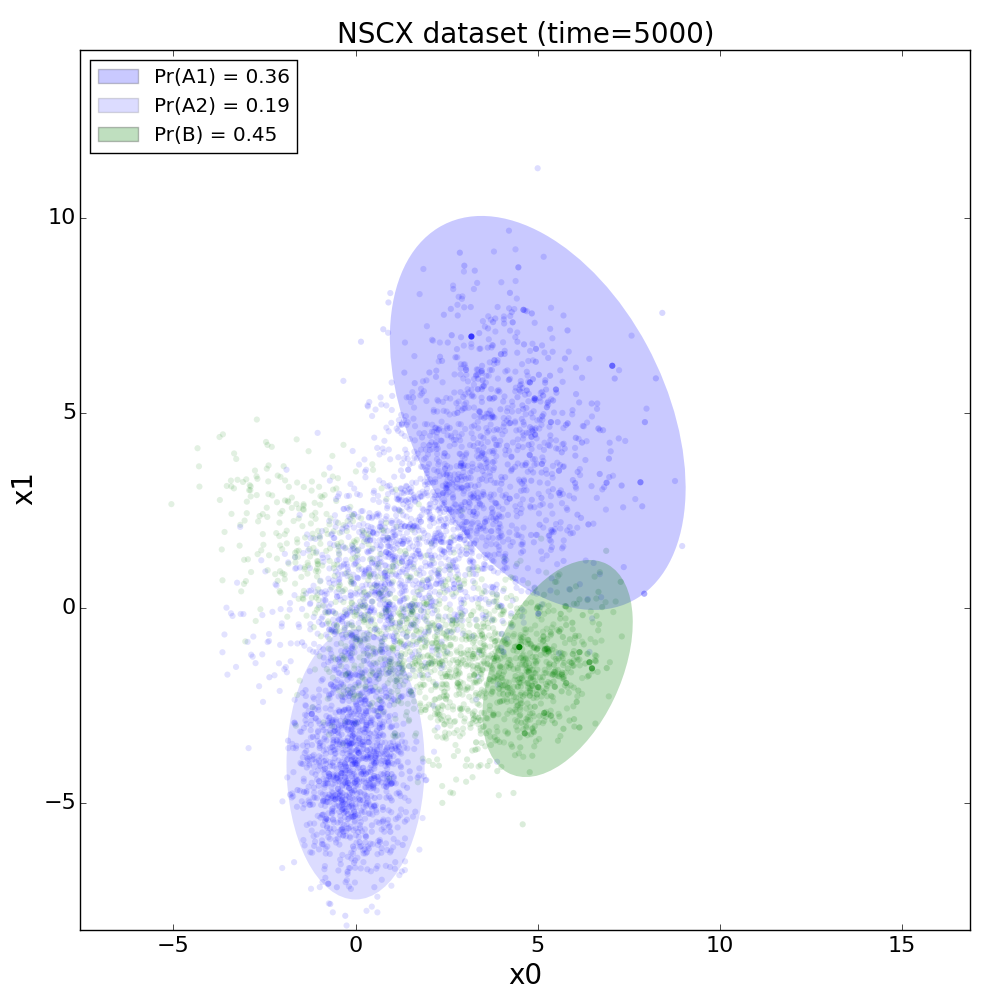
(h) NSCX: Pattern 5000

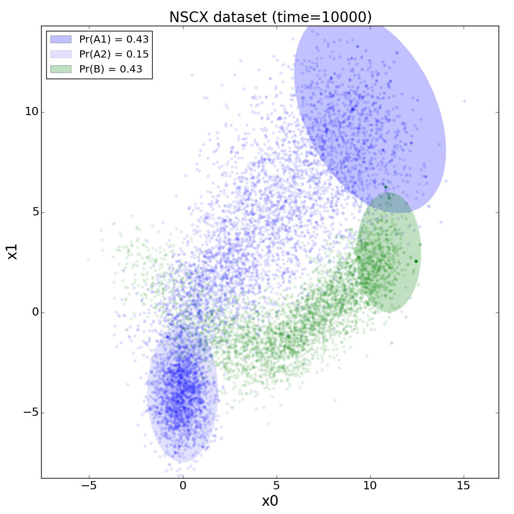
(i) NSCX: Pattern 10000

Figure 1: Graphical description for all the datasets. Blue color is distribution A (or A1 and A2 in some cases) and green is B (B1 and B2). Ellipses are used to represent the distributions at a given point of time, where size is a measure of variance of the distribution. Color intensity is a measure of the a priori probability of the distribution. Patterns are plotted to show the trajectories.

In Table III we can see that DWN and OZAB perform equally well, while NN has a good result if we select the smaller window size (NN¹⁰⁰). Thus, this dataset requires either management of contradiction, or a short time-based memory window. SGD is able to adapt a separation surface to some extent, however, its final accuracy is intermediate. NB is the worst, as expected, as it is not designed to adapt to contradiction in any way.

In addition to the final value of $AE_{preq}$, much information may be extracted from figures that show $AE^{500}_{preq}$. They can be used to show the dynamic behavior of some of the methods, as they average error during a period of time, thus providing clear transitory situations. For instance, Fig. 2a shows that NB is not able to adapt to this type of change at all, as the error increases up to 50% and never recovers.

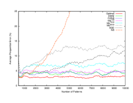
(a) NSGT

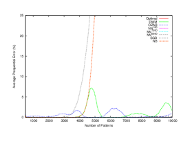
(b) NSGR

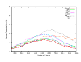
(c) NSLC

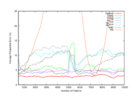
(d) NSGT-I

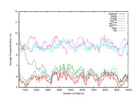
(e) NSPC

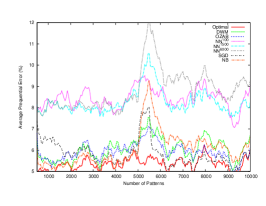
(f) NSPC-A

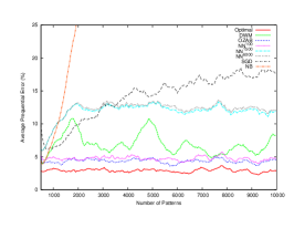
(g) NSGT-F

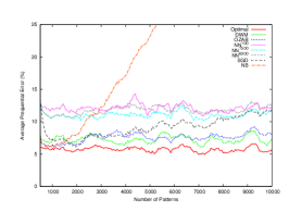
(h) NSGT-5D

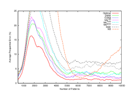
(i) NSCX

Figure 2: Evolution of average prequential error for our datasets, with a window of 500 patterns ($AE^{500}_{preq}(n)$).

With SGD, the error slowly increases over time, so the longer the dataset, the worse for this method. SGD is creating a separation surface that takes into account past data that is no longer valid, and in doing so, it is not really forgetting contradictory data. Ensemble algorithms specifically designed for non-stationary datasets (DWM and OZAB) perform well. Even though their approaches to non-stationarity are different, both are working in this case, and the error tends to be stable after a certain number of patterns. Also NN¹⁰⁰ has a stable $AE^{500}_{preq}$, because it avoids contradiction by taking into account only the most recent data. However, NN is less accurate than other methods when distributions overlap.

Regarding NSGR, Table III shows that the optimal Bayes serious concern to most algorithms as shown by NN¹⁰⁰; it can be classified quite accurately by simply adjusting the memory window to a minimal size, because there is no significant overlap between distributions. In this dataset SGD achieves a second-best performance, because it seems to be able to rotate the plane separating both distributions as needed. On the other hand, having a long-term memory is clearly detrimental, as we can see from NN with a long window (6000) because if all data is retained in the memory, the new data completely contradicts past data. NB is the extreme case of this effect.

Some additional information can be obtained from Fig. 2b. When distributions move close to 90 degrees (pattern 2500) new data contradicts the old data learned at the start. The contradiction reaches a maximum when angle is 180 degrees (pattern 5000). Both periods are clearly shown in Fig. 2b by the behavior of NB, that is unable to adapt to this type of contradiction.

Different algorithms react differently in this moment of change, and the amount of deviation from the original error and the time it takes to revert to a good level of error may be used as a measure of the “inertia” of the algorithms, that is, resistance to change. In checking the values associated with the peaks starting at pattern index 2500 we can deduce that OZAB detects change earlier than DWM and adapts slower. DWM detects change near pattern of index 5000 and is abruptly affected. Then, it rapidly adapts towards a good classification error. SGD is unaffected by this change, so we understand that it is adapting constantly to the new data.

4.2 Contradiction in the Presence of Local Change

The dataset in this section includes different trajectories for each of the distributions. We consider these changes as a local transformation in the input space. In Dataset NSLC, for non-stationary local change, the starting and final distributions can be easily identified, as they begin separately – see for instance Fig. 1c.

When the middle of the sequence has been attained, the distributions overlap and then separate again. Even in the presence of change, the patterns are sampled from distributions that are located roughly on each side of a vertically-oriented decision frontier. This means that a complex representation may not provide much advantage over a very simple one, such as a single linear hyperplane or a NN classifier with a memory composed of just a few patterns. The optimal frontier, however, should perform a rotation of 90 degrees during the sequence to properly classify data.

Table III shows that many algorithms are able to perform well in the NSLC dataset.The less accurate is again NN with the longest sliding window. The reason for the performance of NN⁶⁰⁰⁰ is that a long sliding window size (6000) is unable to forget past knowledge and assigns the wrong class to new data over the end of the dataset.

In this case we can assess that sometimes incremental algorithms not designed for non-stationary data may seem to work well if they are only evaluated using $AE_{preq}$ . Indeed, NB leads to a result similar to that observed for NN in this dataset because it has a good behavior until distributions exchange their positions. The best algorithm is SGD, since this dataset has a simple representation with a surface of separation that changes slowly enough for SGD to adjust to contradiction.

A more detailed analysis (Fig. 2c) reveals some information that is not obvious from the accumulated error measure.

Indeed, around pattern 5000 where the overlap is at a maximum, the error rises above 10% for NN, because NN is the most affected by the increase in the distribution overlap (due to the nearest neighbor sensitivity to noise), but remains close to the optimum for the rest. When the two distributions are separating, all of SGD, DWM and OZAB track the new distributions following the optimal error very closely. Also NN¹⁰⁰ decreases; but the NB error is increasingly separating from the optimal, indicating clearly that even when the overall accuracy is satisfactory, NB is only performing well during the first part of the dataset.

4.3 Long-term Memory

We define long-term memory as the ability of an algorithm to retain what was learned in the past as long as it is not contradictory with more recent learning. To assess this property, we propose the dataset NSGT-I (non-stationary global translation, iterated). This dataset has two phases, each of them based on dataset NSGT. For the first phase, we sampled data for half of the duration (5000 patterns). Then, distributions were reset to their starting positions and we repeated the process.

In Fig. 1a we see how patterns for the first phase are distributed in two diagonal bands when the second phase begins. An algorithm with long term memory might be able to learn the surface of separation and thus improve its results for the second phase of the dataset.

Results in Table III show that OZAB and NN¹⁰⁰ are the best algorithms, and also DWM performs well. However, this seems contradictory to the fact that NN¹⁰⁰ has, by definition, no long term memory.

The difficulty of deciding if the algorithm exhibits long-term memory is that the error metric is not an adequate means of evaluating on this feature. Both phases of the dataset must be compared, which can be done by analysing the average prequential error $AE^{w}_{preq}$ plotted in Fig. 2d.

In this figure we detect different behaviors:

• OZAB and DWM have a peak around pattern 5000, and after some learning they return to acceptable levels of error. That is, the model is not retaining data from the first phase when the second phase begins, and some time is required to adapt to the phase transition.

• NN¹⁰⁰ is unaffected by the transition at pattern 5000. This is a result of the fact that the algorithm takes into account the new patterns for classification immediately, while old patterns in memory are distant from the area where patterns are being observed. That is, the results are not caused by long-term memory, but by instant adaptation.

• In contrast, SGD seems to retain useful information concerning the first part of the algorithm, which accounts for a reduction in error during phase 2. For SGD, the error is abruptly reduced when the second phase begins at its minimum level. We conclude that SGD exhibits a behavior compatible with long term memory.

For direct comparison of the effect of long term memory in NN algorithms, in Fig. 2d we can compare results for NN with different window sizes, compared to the error of NB. The plot indicates that NN⁶⁰⁰⁰ behaved better in the second phase than in the first phase. However, this was not shown in the average error measure as the overall performance was clearly better when the window size was smaller (NN¹⁰⁰).

Also NB exhibits long term memory, as phase 2 has less error than phase 1. The error drops until the Bayes error has been reached at the middle of phase 2 (pattern 7000), where distributions have moved half of their trajectory. This means that in phase 1 an “average” model was learned which was able to perform optimally at this point in time.

4.4 Change in Distribution Frequency

The NSPC dataset contains data from three distributions, two of class A (A1 and A2), one of class B. The class B distribution does not change during the dataset. Distributions of class A undergo a change in a priori probability: at the beginning of the dataset, the one to the right (A2) has a probability of $0.45$ and the one to the left (A1) has a probability of $0.05$ (Fig. 1d). During the dataset, probabilities are slowly exchanged during a time period of 9000 patterns, until the situation is reversed towards the end of the dataset (Fig. 1f). As a priori probabilities for both distributions for class A always sum up to $0.5$, both classes (A and B) are balanced at all times during the dataset.

Table III shows results for this dataset. In Fig. 2e we present the average prequential error ($AE^{500}_{preq}$) for a sliding window of 500 patterns.

In this dataset NB has the best performance, meaning that the slow variation in a priori probabilities is processed adequately and incorporated into its model. Nearest-neighbor approaches lead to the worst results, independently of the window size; however a medium window size (NN¹⁵⁰⁰) seems to provide a slightly better result in these conditions. In addition to NB, the algorithms DWM, OZAB and SGD also follow the optimal Bayes classifier closely. Note that the performance of DWM is much poorer than that of NB, even when its base classifier is NB. This means that the ensemble mechanism is being confused by this dataset.

4.5 Appearance of New Concepts

The NSPC-A dataset is a variation on NSPC. A priori probabilities are not changed slowly, but abruptly, from a starting situation where priors are $0$ for A1 (the leftmost distribution) and $0.5$ for A2 (the rightmost distribution), to the end situation with the opposite situation of $0.5$ (for A1) and $0.0$ (for A2) – see illustration in Fig. 1d, Fig.1e and Fig. 1f.

Table III shows results for this dataset, while Fig. 2f presents the average prequential error for a sliding window of 500 patterns.

The behavior of algorithms for this dataset depends on how they react to the abrupt change, more than the actual difference in the accumulated error, which is similar for all algorithms, except for those based on NN. SGD and OZAB are significantly better than NB, but the difference in accumulated error is small anyway.

Fig. 2f indicates that most of the algorithms perform well during the two “stable” periods at the beginning and the end of the dataset, while reaction to the change in pattern 5000 is very different: NB has a significant increase in error and adapts very slowly towards the end of the dataset; SGD has a high increase, but adapts quickly; DWM has an even smaller increase at the peak, but seems to be unable to adapt completely, since the performance at the end of the dataset is poorer than at the beginning; OZAB exhibits the smallest increase in error, but returns to the levels it had at the beginning.

As with NSPC, nearest-neighbor approaches have the worst results. In Fig. 2f we see that for NN algorithms, the lack of performance is not only related to the transition in pattern 5000, but to problems in separating these distributions that have a high degree of overlap.

4.6 Speed of Change

In this section we investigate the effect of the speed of change in terms of accuracy. For that purpose, we use the dataset NSGT-F (a “fast” version of NSGT), and compare the results with results of the basic (or “slow” version) shown previously. NSGT-F is described by two distributions that undergo a global translation (see Fig. 1a) as in NSGT, but distribution centers are moved three times the distance in each coordinate. The speed of change is thus three times the speed in NSGT.

In Table III, comparison between NSGT-F and the NSGT dataset shows that NB, SGD and DWM have a very significant decrease in performance, while OZAB is mostly unaffected by this change. NN¹⁰⁰ performs better in this case, almost matching the performance of OZAB.

Fig. 2g provides an illustration of the average prequential error for a sliding window of 500 patterns. The trends for NB and SGD were the same as for NSGT, i.e., their error increased towards the end of the dataset. Higher velocity has an important effect because this increase starts earlier and grows at a faster rate. The decrease in accuracy for DWM (which performed well when translation was slow), is caused by peaks of increased error that are later corrected. This can be explained by the mechanism of member creation of the DWM ensemble. In this case, too much error is accumulated until a new ensemble member is activated to adapt to the new data.

4.7 Effect of Dimensionality

Datasets in two dimensions allow visualization, and are thus convenient for inspection and validation of performances. However, behavior of algorithms may change drastically as dimensionality increases given the exponential growth of the input space this generates.

In some research studies, the effect of a dimensionality increase is verified by adding noisy and useless dimensions that must be filtered out by learning methods in order to achieve optimal classification accuracy. We are not considering this case here as we believe this to be a problem of feature selection/extraction, which may be dealt with using other techniques designed for that purpose. Instead, we are including additional dimensions that are useful and informative, with changes over the distributions of the data that are performed over all these dimensions.

The NSGT-5D dataset is based on the NSGT dataset presented in Sec. 4.1, with distributions this time defined in a 5D input space and a translation of the distributions over the time steps parallel to the vector $[1.0\,1.0\,1.0\,1.0\,1.0]$.

The 2-D projection of the distributions and their movement would be similar to that of NSGT (see Fig. 1a).

The covariance matrices parametrizing the distributions have been adjusted to ensure that there is a significant overlap between the distributions. The amount of overlap was estimated by the error of the optimal Bayes classifier and tuned to be similar to the one reported for NSGT. We used symmetrical distributions for simplicity.

It is expected that some algorithms require more patterns to be able to model a distribution as dimension grows. However, increasing the number of patterns would decrease the speed at which the distributions are moving in the input space. We adjusted the distance moved by the distribution centers to ensure that the dataset NSGT-5D use the same number of patterns ($10000$), and that the speed of movement remains equal to the speed in NSGT.

Table III presents the results obtained for NSGT-5D, while Fig. 2h presents the evolution of its prequential error over time.

These results are similar to the results obtained for NSGT, except for the fact that the performance of the NN algorithms decreased for NN¹⁰⁰, while NN⁶⁰⁰⁰ remained unaffected. This is expected due to the known dimensionality issues of the NN rule. This means that in these types of algorithms the window size must be adjusted to take into account both change and dimensionality at the same time.

As in the case of NSGT, the algorithms DWM and OZAB exhibited better performance than that of SGD, especially if we consider the last part of the dataset where SGD is increasing its error. So even with an increase in dimensions, the former results are generally applicable to these algorithms.

4.8 Complex Non-stationary Changes

Finally, we introduce the dataset NSCX that combines several types of changes. This dataset has two initial distributions (A1 and A2) (Fig. 1g) that are then separated by a third one (B) which appears gradually (change in prior) and translates downwards (local change) while A2 moves diagonally. A1 and A2 exchange their a priori probabilities gradually. We also perform a rotation of distributions A1 and B, and the variance of A1 grows with time. Note that, contrary to the previous datasets, during part of the evolution of the dataset, distributions are non-separable by a single hyperplane (Fig. 1h), but towards the end they can easy be separated with a linear frontier (Fig. 1i).

Table III presents the results obtained for the NSCX dataset, while Fig. 2i presents the evolution of its prequential error over time.

Overall, OZAB is the best algorithm followed by DWM and NN¹⁰⁰ which are able to provide good results. However, SGD is unable to perform much better than NB. It must be noted that OZAB and NN are the algorithms that, in general terms, are able to classify distributions with more complex representations.

The plot for the optimal error (see Fig. 2i) indicates that the distributions increasingly overlap during the first part of the dataset but then become separated again. This improves the overall behavior of the NN algorithms towards the end. While the final situation seems to be an “easy” situation, that is, it is linearly separable (Fig.1i), SGD is not able to evolve towards a linear separation frontier. At the end of the dataset, DWM shows no adaptation towards the optimal classifer error.

5 Summary of Results

For a proper assessment of Non-Stationary Learning (NSL) methods, we are proposing a methodology that includes: several datasets that test different features of the methods; datasets with parameters that allow the speed of change to be varied; metrics that are able to discard averaging effects of the accumulated error rate (i.e., average prequential error with a sliding window).

The NSGT dataset indicates that, as expected, NB is not designed to adapt to even global change, that is, the simplest type of change involving global displacement in the input space with no relative change. For SGD we showed that error increases with time. OZAB and DWM can deal with contradiction by adapting their internal model, either instance weights (OZAB) or member weights (DWM) when their accuracy is reduced. Also NN¹⁰⁰ achieves good results with a simple time-based forgetting mechanism.

NSGR shows that if a very simple representation is enough to represent data (SGD, NN¹⁰⁰), then simple algorithms may work better than complex ones (OZAB, DWM).

For local change (NSLC), SGD was shown as a good option that was able to adapt to transitory increase in complexity. It can also generate a very exact linear separation between overlapping distributions that can rotate as the distributions intersect. NN approaches, on the other side, are much less tolerant to overlap and are affected in a greater proportion when the Bayes error increases.

The NSGT-I dataset was specifically designed to test which methods can recall models created early during learning. We were able to detect this feature in NB, SGD, and in the version of NN that had a longer memory window.

Change in a priori probability was well processed by all algorithms when it was gradual (NSPC). However, abruptly introducing change (NSPC-A) induces different behaviors depending on the inertia and adaptability of the different algorithms. Here, OZAB was very successful but slow to adapt, while SGD was greatly perturbed by the change, but was able to rapidly adapt later.

Concerning speed of change, the behavior of the analyzed algorithms can be evaluated using our methodology. For instance, when changes occurs more rapidly (NSGT-F dataset), it appears that SGD is unable to retain its good results due to its accumulative increase in error. Also DWM seems to have more difficulty in adapting to rapid change than OZAB, while for NN algorithms this depends on the window size: as expected, a small window size is adequate for rapid adaptation.

The dataset NSGT-5D, with its extra dimension, also shows some of the well-known features of the algorithms. Behavior in two dimensions does not always carry-on to input spaces of higher dimensions, specially for NN, where the smaller window size, that was capable of adaptating very well to change in many situations, is unable to maintain the good results it has for the 2-dimensional version of this dataset.

Finally, the dataset NSCX can be used to evaluate representation issues and complex situations. In this context NN seemed to be a good option, except when overlap between distributions of two classes increases. The SGD algorithm relies on a linear discriminant, and thus would not be able to cope with non-linearly separable datasets such as NSCX. This weakness is clear in Fig. 2i where SGD was unable to perform well once the third distribution was introduced. Both OZAB and DWM were able to perform reasonably well.

Overall OZAB and DWM were the most flexible and accurate NSL algorithms. They have an equilibrium between error (usually lower for OZAB) and speed (DWM has a much lower computational cost). SGD was able to perform well when the representation of the separation surface is simple and change is slow. NN with a short memory window can be competitive and is flexible enough for any type of surface of separation or velocity of change, but it is adversely affected both by noise (overlap between distributions) and the dimensionality of the problem.

6 Conclusions

This paper presents a testbed for the evaluation of algorithms in the field of Incremental Learning from Non-Stationary data (NSL). This task is defined in relation to other fields that share some characteristics. Specifically we refer to these algorithms as incremental learning algorithms and they must deal with sequential data, continuous flow, and non-stationary distributions.

This field has no definite criteria for comparison. The analysis of the state of the art shows that authors are comparing algorithms using datasets that were not initially oriented towards NSL. Also, the basic characteristics of these datasets such as the amount and speed of change remain undefined. This means that we cannot determine which features of an algorithm are being tested when we claim that a method provides good results on one of the datasets in the literature.

Most of our work has been oriented towards the identification of the most relevant tests that have to be performed in order to determine if a proposed incremental learning algorithm will be able to perform the task at hand. These tests include contradiction, long-term memory, local distribution invariance, global distribution invariance, data frequency invariance, adaptation to new data, dimensionality invariance, and velocity invariance.

We have created artificial datasets where each of the former tests can be performed independently. Experiments have been performed using these datasets and well-known algorithms. Results confirm that our testbed can be used to compare candidate algorithms in a generic way. The discussion of the results also provides guidelines on how metrics should be interpreted.

Alejandro Cervantes graduated as Telecommunications Engineer at Universidad Politécnica of Madrid (Spain), in 1993. He received his PhD in Computer Science at Carlos III of Madrid in 2007. He is currently an assistant professor at the Computer Science Department at this same University. His current interests focus in algorithms for classification of non-stationary data, large multi-objective optimization problems, and swarm intelligence algorithms for data mining.

Christian Gagné received a B.Ing. in Computer Engineering and a PhD in Electrical Engineering from Université Laval in 2000 and 2005, respectively. He is professor of Computer Engineering at Université Laval since 2008. His research interests are on the engineering of intelligent systems, in particular systems involving machine learning and evolutionary computation. He is member of the editorial board of Genetic Programming and Evolvable Machines, and participated in the organization of several conferences.

Pedro Isasi is engineer in Computer Science for Polytechnic University of Madrid since 1991 and received his PhD at this same university in 1994. From 2001, he is a Professor in Computer Science at Carlos III of Madrid University. He is funder and director of the Neural Network and Evolutionary Computation Laboratory. His principal researches are in the field of Machine Learning, Metaheuristics and evolutionary optimization methods, mainly applied to prediction and classification.

Marc Parizeau Marc Parizeau is a professor of Computer Engineering at Université Laval, Québec City. He obtained his Ph.D. in 1992 from École Polytechnique de Montréal. His research interests are in the field of intelligent systems, in machine learning for pattern recognition in particular, parallel and distributed systems. In 2008, he created a High Performance Computing center at Université Laval, and is the current scientific Director of Calcul Québec, one of the four regional divisions of Compute Canada, the national HPC platform.

References

- [1] C. Giraud-Carrier, “A note on the utility of incremental learning,” AI Communications, vol. 13, no. 4, pp. 215–223, December 2000.
- [2] D. P. Helmbold and P. M. Long, “Tracking drifting concepts by minimizing disagreements,” Machine Learning, vol. 14, pp. 27–45, January 1994.
- [3] L. Bottou and O. Bousquet, “Learning using large datasets,” in Mining Massive DataSets for Security, ser. NATO ASI Workshop Series. Amsterdam: IOS Press, 2008, pp. 15–26.
- [4] M. Kholghi, H. Hassanzadeh, and M. Keyvanpour, “Classification and evaluation of data mining techniques for data stream requirements,” in Proc. of International Symposium on Computer Communication Control and Automation (3CA ’10), vol. 1, may 2010, pp. 474 –478.
- [5] P. Domingos and G. Hulten, “Mining high-speed data streams,” in Proc. of the 6th ACM SIGKDD international conference on Knowledge discovery and data mining (KDD ’06). New York, NY, USA: ACM, 2000, pp. 71–80.
- [6] D. W. Aha and D. Kibler, “Instance-based learning algorithms,” in Machine Learning, 1991, pp. 37–66.
- [7] R. Elwell and R. Polikar, “Incremental learning of concept drift in nonstationary environments,” IEEE Transactions on Neural Networks, vol. 22, no. 10, pp. 1517–1531, 2011.
- [8] W. N. Street and Y. Kim, “A streaming ensemble algorithm (SEA) for large-scale classification,” in Proc. of ACM SIGKDD international conference on Knowledge discovery and data mining (KDD ’01). New York, NY, USA: ACM, 2001, pp. 377–382.
- [9] J. a. Gama, R. Sebastião, and P. P. Rodrigues, “Issues in evaluation of stream learning algorithms,” in Proc. of the 15th ACM SIGKDD international conference on Knowledge discovery and data mining (KDD ’09). New York, NY, USA: ACM, 2009, pp. 329–338.
- [10] D. Martínez-Rego, B. Pérez-Sánchez, O. Fontenla-Romero, and A. Alonso-Betanzos, “A robust incremental learning method for non-stationary environments,” Neurocomputing, vol. 74, no. 11, pp. 1800 – 1808, 2011.
- [11] G. Carpenter and S. Grossberg, “The ART of adaptive pattern recognition by a self-organizing neural network,” Computer, vol. 21, no. 3, pp. 77 –88, mar 1988.
- [12] C. Alippi and M. Roveri, “Just-in-time adaptive classifiers part I: Detecting nonstationary changes,” IEEE Transactions on Neural Networks, vol. 19, no. 7, pp. 1145–1153, jul 2008.
- [13] A. Bifet, B. Pfahringer, J. Read, and G. Holmes, “Efficient data stream classification via probabilistic adaptive windows,” in Proc. of the 28th Annual ACM Symposium on Applied Computing (SAC ’13). New York, NY, USA: ACM, 2013, pp. 801–806.
- [14] G. Hulten, L. Spencer, and P. Domingos, “Mining time-changing data streams,” in Proc. of the 7th ACM SIGKDD international conference on Knowledge discovery and data mining (KDD ’01). New York, NY, USA: ACM, 2001, pp. 97–106.
- [15] L. Minku and X. Yao, “DDD: A new ensemble approach for dealing with concept drift,” IEEE Transactions on Knowledge and Data Engineering, vol. 24, no. 4, pp. 619–633, April 2012.
- [16] M. Muhlbaier and R. Polikar, “Multiple classifiers based incremental learning algorithm for learning in nonstationary environments,” in Proc. of the International Conference on Machine Learning and Cybernetics (ICMLC ’08), vol. 6, aug 2007, pp. 3618 –3623.
- [17] M. Muhlbaier, A. Topalis, and R. Polikar, “Learn++.NC: Combining ensemble of classifiers with dynamically weighted consult-and-vote for efficient incremental learning of new classes,” IEEE Transactions on Neural Networks, vol. 20, no. 1, pp. 152–168, jan. 2009.
- [18] N. C. Oza, “Online ensemble learning,” Ph.D. dissertation, The University of California, Berkeley, CA, Sep 2001.
- [19] A. Pocock, P. Yiapanis, J. Singer, M. Luján, and G. Brown, “Online non-stationary boosting,” Lecture Notes in Computer Science, vol. 5997, pp. 205–214, 2010.
- [20] A. Bifet, G. Holmes, B. Pfahringer, R. Kirkby, and R. Gavaldà, “New ensemble methods for evolving data streams,” in Proceedings of the 15th ACM SIGKDD international conference on Knowledge discovery and data mining (KDD ’09). New York, NY, USA: ACM, 2009, pp. 139–148.
- [21] M. Riekert, K. Malan, and A. Engelbrect, “Adaptive genetic programming for dynamic classification problems,” in IEEE Congress on Evolutionary Computation (CEC ’09), may 2009, pp. 674 –681.
- [22] B. Fritzke, “Fast learning with incremental RBF networks,” in Neural Processing Letters, vol. 1, 1994, pp. 2–5.
- [23] Y. Prudent and A. Ennaji, “An incremental growing neural gas learns topologies,” in Proceedings of the 2005 IEEE International Joint Conference on Neural Networks (IJCNN ’05), vol. 2, july-aug 2005, pp. 1211 – 1216.
- [24] Y. Xu, S. Furao, O. Hasegawa, and J. Zhao, “An online incremental learning vector quantization,” in Proceedings of the 13th Pacific-Asia Conference on Advances in Knowledge Discovery and Data Mining (PAKDD ’09). Berlin, Heidelberg: Springer-Verlag, 2009, pp. 1046–1053.
- [25] G. Cauwenberghs and T. Poggio, “Incremental and Decremental Support Vector Machine Learning,” in Proc. of Advances in Neural Information Processing Systems (NIPS ’00), 2000, pp. 409–415.
- [26] P. Laskov, C. Gehl, S. Krüger, K.-r. Müller, K. Bennett, and E. Parrado-hern, “Incremental support vector learning: Analysis, implementation and applications,” Journal of Machine Learning Research, vol. 7, p. 2006, 1968.
- [27] L. Bottou, “Large-scale machine learning with stochastic gradient descent,” in Proceedings of the 19th International Conference on Computational Statistics (COMPSTAT’2010), Y. Lechevallier and G. Saporta, Eds. Paris, France: Springer, August 2010, pp. 177–187.
- [28] A. Tsymbal, “The problem of concept drift: Definitions and related work,” Department of Computer Science, Trinity College: Dublin, Ireland, Tech. Rep., 2004.
- [29] A. Kuh and T. Petsche, “Learning time varying concepts with applications to pattern recognition problems,” in Proc. of the Conference on Signals, Systems and Computers (SS&C ’90), vol. 2, nov 1990, p. 971.
- [30] D. P. Helmbold and P. M. Long, “Tracking drifting concepts using random examples,” in Proc. of the annual workshop on Computational learning theory (COLT ’91). San Francisco, CA, USA: Morgan Kaufmann Publishers Inc., 1991, pp. 13–23.
- [31] G. Widmer and M. Kubat, “Learning in the presence of concept drift and hidden contexts,” in Machine Learning, vol. 23, 1996, pp. 69–101.
- [32] M. Last, “Online classification of nonstationary data streams,” Intellingence Data Analysis, vol. 6, pp. 129–147, April 2002.
- [33] L. Cohen, G. Avrahami, M. Last, A. Kandel, and O. Kipersztok, “Incremental Classification of Nonstationary Data Streams,” in Proc. of the International Workshop on Knowledge Discovery in Data Streams, 2005, pp. 117–124.
- [34] L. Cohen, G. Avrahami-Bakish, M. Last, A. Kandel, and O. Kipersztok, “Real-time data mining of non-stationary data streams from sensor networks,” Information Fusion, vol. 9, no. 3, pp. 344 – 353, 2008, special Issue on Distributed Sensor Networks.
- [35] R. Klinkenberg, “Learning drifting concepts: Example selection vs. example weighting,” Intelligent Data Analysis, vol. 8, no. 3, pp. 281–300, Aug. 2004.
- [36] A. P. Dawid, “Statistical theory: The prequential approach,” Journal of the Royal Statistical Society-A, vol. 147, pp. 278–292, 1984.
- [37] S. Chen and H. He, “Towards incremental learning of nonstationary imbalanced data stream: a multiple selectively recursive approach,” Evolving Systems, vol. 2, pp. 35–50, 2011.
- [38] A. Shaker and E. Hüllermeier, “Recovery analysis for adaptive learning from non-stationary data streams: Experimental design and case study,” Neurocomputing, vol. 150, Part A, no. 0, pp. 250 – 264, 2015.
- [39] A. Bifet, J. Read, I. Žliobaitė, B. Pfahringer, and G. Holmes, “Pitfalls in benchmarking data stream classification and how to avoid them,” in Machine Learning and Knowledge Discovery in Databases, ser. Lecture Notes in Computer Science, H. Blockeel, K. Kersting, S. Nijssen, and F. Železný, Eds. Springer Berlin Heidelberg, 2013, vol. 8188, pp. 465–479.
- [40] J. C. Schlimmer and R. H. Granger, Jr., “Incremental learning from noisy data,” Machine Learning, vol. 1, pp. 317–354, mar 1986.
- [41] L. Breiman, J. H. Friedman, R. A. Olshen, and C. J. Stone, Classification and regression trees. New York, N.Y: CRC Press, 1999.
- [42] S. M. Lee and S. J. Roberts, “Sequential dynamic classification using latent variable models,” The Computer Journal, vol. 53, pp. 1415–1429, November 2010.
- [43] M. Harries, “SPLICE-2 comparative evaluation: Electricity pricing,” University of New South Wales, Tech. Rep., 1999.
- [44] D. R. Lowne, S. J. Roberts, and R. Garnett, “Sequential non-stationary dynamic classification with sparse feedback,” Pattern Recognition, vol. 43, pp. 897–905, mar 2010.
- [45] A. Bifet, G. Holmes, B. Pfahringer, P. Kranen, H. Kremer, T. Jansen, and T. Seidl, “MOA: Massive online analysis, a framework for stream classification and clustering,” Journal of Machine Learning Research - Proceedings Track, vol. 11, pp. 44–50, 2010.
- [46] J. Z. Kolter and M. A. Maloof, “Dynamic weighted majority: An ensemble method for drifting concepts,” The Journal of Machine Learning Research, vol. 8, pp. 2755–2790, December 2007.