Arnoldi decomposition, GMRES, and preconditioning
for linear discrete ill-posed problems

Abstract

GMRES is one of the most popular iterative methods for the solution of large linear systems of equations that arise from the discretization of linear well-posed problems, such as Dirichlet boundary value problems for elliptic partial differential equations. The method is also applied to iteratively solve linear systems of equations that are obtained by discretizing linear ill-posed problems, such as many inverse problems. However, GMRES does not always perform well when applied to the latter kind of problems. This paper seeks to shed some light on reasons for the poor performance of GMRES in certain situations, and discusses some remedies based on specific kinds of preconditioning. The standard implementation of GMRES is based on the Arnoldi process, which also can be used to define a solution subspace for Tikhonov or TSVD regularization, giving rise to the Arnoldi–Tikhonov and Arnoldi-TSVD methods, respectively. The performance of the GMRES, the Arnoldi–Tikhonov, and the Arnoldi-TSVD methods is discussed. Numerical examples illustrate properties of these methods.

1 Introduction

This paper considers the solution of linear systems of equations

$$A\mathbf{x}=\mathbf{b},\qquad A\in{{\mathbb{C}}}^{m\times m},\qquad\mathbf{x},\mathbf{b}\in{{\mathbb{C}}}^{m},$$ (1)

with a large matrix $A$ with many “tiny” singular values of different orders of magnitude. In particular, $A$ is severely ill-conditioned and may be rank-deficient. Linear systems of equations (1) with a matrix of this kind are commonly referred to as linear discrete ill-posed problems. They arise, for instance, from the discretization of linear ill-posed problems, such as Fredholm integral equations of the first kind with a smooth kernel.

In many linear discrete ill-posed problems that arise in science and engineering, the right-hand side vector $\mathbf{b}$ is determined through measurements and is contaminated by a measurement error $\mathbf{e}\in{\mathbb{C}}^{m}$. Thus,

$$\mathbf{b}=\mathbf{b}_{\rm exact}+\mathbf{e},$$ (2)

where $\mathbf{b}_{\rm exact}\in{{\mathbb{C}}}^{m}$ denotes the unknown error-free right-hand side associated with $\mathbf{b}$. We will assume that $\mathbf{b}_{\rm exact}$ is in the range of $A$, denoted by ${\mathcal{R}}(A)$, because this facilitates the use of the discrepancy principle to determine a suitable value of a regularization parameter; see below for details. The error-contaminated right-hand side $\mathbf{b}$ is not required to be in ${\mathcal{R}}(A)$.

We would like to compute the solution of minimal Euclidean norm, $\mathbf{x}_{\rm exact}$, of the consistent linear discrete ill-posed problem

$$A\mathbf{x}=\mathbf{b}_{\rm exact}.$$ (3)

Since the right-hand side $\mathbf{b}_{\rm exact}$ is not known, we seek to determine an approximation of $\mathbf{x}_{\rm exact}$ by computing an approximate solution of the available linear system of equations (1). We note that due to the severe ill-conditioning of the matrix $A$ and the error $\mathbf{e}$ in $\mathbf{b}$, the least-squares solution of minimal Euclidean norm of (1) generally is not a useful approximation of $\mathbf{x}_{\rm exact}$.

A popular approach to determine a meaningful approximation of $\mathbf{x}_{\rm exact}$ is to apply an iterative method to the solution of (1) and terminate the iterations early enough so that the error in $\mathbf{b}$ is not significantly propagated into the computed approximate solution. The most popular iterative methods for the solution of large linear discrete ill-posed problems are LSQR by Paige and Saunders [21, 25, 28, 51], which is based on partial Golub–Kahan decomposition of $A$, and GMRES [7, 8, 23], which is based on partial Arnoldi decomposition of $A$. Here “GMRES” refers to both the standard GMRES method proposed by Saad and Schultz [58] as well as to variants that have been found to perform better when applied to the solution of linear discrete ill-posed problems; see, e.g., [19, 33, 41] for examples.

The LSQR method requires the evaluation of two matrix-vector products in each iteration, one with $A$ and one with its conjugate transpose, which we denote by $A^{*}$. GMRES only demands the computation of one matrix-vector product with $A$ per iteration. This makes GMRES attractive to use when it is easy to evaluate matrix-vector products with $A$ but not with $A^{*}$. This is, for instance, the case when $A$ approximates a Fredholm integral operator of the first kind and matrix-vector products with $A$ are evaluated by a multipole method. Then $A$ is not explicitly formed and matrix-vector products with $A^{*}$ are difficult to compute; see, e.g., [24] for a discussion on the multipole method. It may be difficult to evaluate matrix-vector products with $A^{*}$ also when solving nonlinear problems and $A$ represents a Jacobian matrix, whose entries are not explicitly computed; see [14] for a discussion on such a solution method.

The fact that GMRES does not require the evaluation of matrix-vector products with $A^{*}$ leads to that for many linear discrete ill-posed problems (1), this method requires fewer matrix-vector product evaluations than LSQR to determine a desired approximate solution, see, e.g., [4, 5, 8] for illustrations, as well as [6] for related examples. However, there also are linear discrete ill-posed problems (1), whose solution with LSQR requires fewer matrix-vector product evaluations than GMRES, or for which LSQR furnishes a more accurate approximation of $\mathbf{x}_{\rm exact}$ than GMRES; see below for illustrations, as well as [30]. Reasons for poor performance of GMRES include:

1. The low-dimensional solution subspaces used by GMRES are poorly suited to represent $\mathbf{x}_{\rm exact}$. It is often not possible to rectify this problem by carrying out many iterations, since this typically results in severe propagation of the error $\mathbf{e}$ in $\mathbf{b}$ into the iterates determined by GMRES.

2. The desired solution $\mathbf{x}_{\rm exact}$ may be approximated accurately in solution subspaces generated by GMRES, but the method determines iterates that furnish poor approximations of $\mathbf{x}_{\rm exact}$.

3. The GMRES iterates suffer from contamination of propagated error due to the fact that the initial vector in the Arnoldi decomposition used for the solution of (1) is a normalization of the error-contaminated vector $\mathbf{b}$.

It is the purpose of the present paper to discuss the above mentioned shortcomings of GMRES, illustrate situations when they occur, and provide some remedies. Section 2 defines the Arnoldi process and GMRES, and shows that the solution subspaces used by GMRES may be inappropriate. Also LSQR is briefly discussed, and distances to relevant classes of matrices are introduced. In Section 3, we define the set of generalized Hermitian matrices and the set of generalized Hermitian positive semidefinite matrices. The distance of the matrix $A$ in (1) to these sets sheds light on how quickly GMRES applied to the solution of the linear system of equations (1) will converge. Section 4 describes “preconditioning techniques.” The “preconditioners” discussed do not necessarily reduce the condition number, and they are not guaranteed to reduce the number of iterations. Instead, they are designed to make the matrix of the preconditioned linear system of equations closer the set of generalized Hermitian positive semidefinite matrices. This often results in that the computed solution is a more accurate approximation of $\mathbf{x}_{\rm exact}$ than approximate solutions of the unpreconditioned linear system (1). In Section 5 we consider the situation when GMRES applied to the solution of (1) yields poor approximations of $\mathbf{x}_{\rm exact}$, but the solution subspace generated by the Arnoldi process contains an accurate approximation of $\mathbf{x}_{\rm exact}$. We propose to carry out sufficiently many steps of the Arnoldi process and compute an approximation of $\mathbf{x}_{\rm exact}$ in the solution subspace generated by Tikhonov regularization or truncated singular value decomposition. Both regularization methods allow the use of a solution subspace of larger dimension than GMRES. A few computed examples that illustrate the discussion of the previous sections are presented in Section 6, and Section 7 contains concluding remarks.

2 GMRES for linear discrete ill-posed problems

GMRES is a popular iterative method for the solution of large linear systems of equations with a square nonsymmetric matrix (1) that arise from the discretization of well-posed problems; see, e.g., Saad [57]. The $k$th iterate, $\mathbf{x}_{k}$, determined by GMRES, when applied to the solution of (1) with initial iterate $\mathbf{x}_{0}=\mathbf{0}$, satisfies

$$\|A\mathbf{x}_{k}-\mathbf{b}\|=\min_{\mathbf{x}\in{{\mathbb{K}}}_{k}(A,\mathbf{b})}\|A\mathbf{x}-\mathbf{b}\|,\qquad\mathbf{x}_{k}\in{{\mathbb{K}}}_{k}(A,\mathbf{b}),$$ (4)

where

$${{\mathbb{K}}}_{k}(A,\mathbf{b})=\mbox{span}\{\mathbf{b},A\mathbf{b},\ldots,A^{k-1}\mathbf{b}\}$$

is a Krylov subspace and $\|\cdot\|$ denotes the Euclidean vector norm. We tacitly assume that $k$ is sufficiently small so that $\mbox{dim}({{\mathbb{K}}}_{k}(A,\mathbf{b}))=k$, which in turn guarantees that the iterate $\mathbf{x}_{k}$ is uniquely defined. We will throughout this section assume that $1\leq k\ll m$. The standard implementation of GMRES [57, 58] is based on the Arnoldi process, here given with the modified Gram–Schmidt implementation.

Algorithm 1.

The Arnoldi process

0.	Input $A\in{\mathbb{C}}^{m\times m}$, ${\mathbf{b}}\in{\mathbb{C}}^{m}\backslash\{\mathbf{0}\}$
1.	$\mathbf{v}_{1}:=\mathbf{b}/\|\mathbf{b}\|$;
2.	for $j=1,2,\ldots,k$ do
3.		$\mathbf{w}:=A{\mathbf{v}}_{j}$;
4.		for $i=1,2,\ldots j$ do
5.			$h_{i,j}:={\mathbf{v}}_{i}^{*}\mathbf{w}$; $\mathbf{w}:=\mathbf{w}-{\mathbf{v}}_{i}h_{i,j}$;
6.		end for
7.		$h_{j+1,j}:=\|\mathbf{w}\|$; $\mathbf{v}_{j+1}:=\mathbf{w}/h_{j+1,j}$;
8.	end for

Algorithm 1 generates orthonormal vectors $\mathbf{v}_{1},\mathbf{v}_{2},\ldots,\mathbf{v}_{k+1}$, the first $k$ of which form a basis for ${{\mathbb{K}}}_{k}(A,\mathbf{b})$. Define the matrices $V_{k}=[\mathbf{v}_{1},\mathbf{v}_{2},\ldots,\mathbf{v}_{k}]$ and $V_{k+1}=[V_{k},\mathbf{v}_{k+1}]$. The scalars $h_{i,j}$ determined by the algorithm define an upper Hessenberg matrix $H_{k+1,k}\in{{\mathbb{C}}}^{(k+1)\times k}$, i.e., the $h_{i,j}$ are the nontrivial entries of $H_{k+1,k}$. Using these matrices, the recursion formulas for the Arnoldi process can be expressed as a partial Arnoldi decomposition,

$$AV_{k}=V_{k+1}H_{k+1,k}.$$ (5)

The above relation is applied to compute the GMRES iterate $\mathbf{x}_{k}$ as follows: Express (4) as

$$\min_{\mathbf{x}\in{{\mathbb{K}}}_{k}(A,\mathbf{b})}\|A\mathbf{x}-\mathbf{b}\|=\min_{\mathbf{y}\in{{\mathbb{C}}}^{k}}\|AV_{k}\mathbf{y}-\mathbf{b}\|=\min_{\mathbf{y}\in{{\mathbb{C}}}^{k}}\|H_{k+1,k}\mathbf{y}-\mathbf{e}_{1}\|\mathbf{b}\|\,\|,$$ (6)

where the orthonormality of the columns of $V_{k}$ and the fact that $\mathbf{b}=V_{k+1}\mathbf{e}_{1}\|\mathbf{b}\|$ have been exploited. Throughout this paper $\mathbf{e}_{j}=[0,\ldots,0,1,0,\ldots,0]^{*}$ denotes the $j$th axis vector. The small minimization problem on the right-hand side of (6) can be solved conveniently by QR factorization of $H_{k+1,k}$; see [57]. Denote the solution by $\mathbf{y}_{k}$. Then $\mathbf{x}_{k}=V_{k}\mathbf{y}_{k}$ solves (4) and $\mathbf{r}_{k}=\mathbf{b}-A\mathbf{x}_{k}$ is the associated residual error. Since ${{\mathbb{K}}}_{k-1}(A,\mathbf{b})\subset{{\mathbb{K}}}_{k}(A,\mathbf{b})$, we have $\|\mathbf{r}_{k}\|\leq\|\mathbf{r}_{k-1}\|$; generally this inequality is strict. Note that $\|\mathbf{r}_{k}\|=\|\mathbf{e}_{1}\|\mathbf{b}\|-H_{k+1,k}\mathbf{y}_{k}\|$, so that the norm of the residual vector can be monitored using projected quantities, which are inexpensive to compute. We remark that a reorthogonalization procedure can be considered with Algorithm 1, by running an additional modified Gram–Schmidt step for the vector $\mathbf{w}$ after step 6 has been performed: this has the effect of assuring the columns of $V_{k+1}$ a better numerical orthogonality.

Assume that a fairly accurate bound $\delta>0$ for the norm of the error $\mathbf{e}$ in $\mathbf{b}$ is available,

$$\|\mathbf{e}\|\leq\delta,$$ (7)

and let $\tau\geq 1$ be a user-chosen parameter that is independent of $\delta$. The discrepancy principle prescribes the iterations of GMRES applied to the solution of (1) to be terminated as soon as an iterate $\mathbf{x}_{k}$ has been determined such that the associated residual error $\mathbf{r}_{k}$ satisfies

$$\|\mathbf{r}_{k}\|\leq\tau\delta.$$ (8)

The purpose of this stopping criterion is to terminate the iterations before the iterates $\mathbf{x}_{k}$ are severely contaminated by propagated error that stems from the error $\mathbf{e}$ in $\mathbf{b}$. Note that the residual $\mathbf{r}_{\rm exact}=\mathbf{b}-A\mathbf{x}_{\rm exact}$ satisfies the inequality (8). This follows from the consistency of (3), and (7). Also iterations with LSQR are commonly terminated with the discrepancy principle; see, e.g., [7, 21, 25] for discussions on the use of the discrepancy principle for terminating iterations with GMRES and LSQR.

The LSQR method [51] is an implementation of the conjugate gradient method applied to the normal equations,

$$A^{*}A\mathbf{x}=A^{*}\mathbf{b},$$ (9)

with a Hermitian positive semidefinite matrix. LSQR circumvents the explicit formation of $A^{*}A$. When using the initial iterate $\mathbf{x}_{0}=\mathbf{0}$, LSQR determines approximate solutions of (1) in a sequence of nested Krylov subspaces ${{\mathbb{K}}}_{k}(A^{*}A,A^{*}\mathbf{b})$, $k=1,2,\ldots~{}$. The $k$th iterate, $\mathbf{x}_{k}$, computed by LSQR satisfies

$$\|A\mathbf{x}_{k}-\mathbf{b}\|=\min_{\mathbf{x}\in{{\mathbb{K}}}_{k}(A^{*}A,A^{*}\mathbf{b})}\|A\mathbf{x}-\mathbf{b}\|,\qquad\mathbf{x}_{k}\in{{\mathbb{K}}}_{k}(A^{*}A,A^{*}\mathbf{b});$$

see [2, 51] for further details on LSQR.

When $\delta$ in (7) is fairly large, only few iterations can be carried out by GMRES or LSQR before (8) is satisfied. In particular, an accurate approximation of $\mathbf{x}_{\rm exact}$ can then be determined by GMRES only if $\mathbf{x}_{\rm exact}$ can be approximated well in a low-dimensional Krylov subspace ${{\mathbb{K}}}_{k}(A,\mathbf{b})$. Moreover, it has been observed that GMRES based on the Arnoldi process applied to $A$ with initial vector $\mathbf{b}$ may determine iterates $\mathbf{x}_{k}$ that are contaminated by more propagated error than iterates generated by LSQR; see [30]. A reason for this is that a normalization of the error-contaminated vector $\mathbf{b}$ is the first column of the matrix $V_{k}$ in the Arnoldi decomposition (5), and the error $\mathbf{e}$ in $\mathbf{b}$ is propagated to all columns of $V_{k}$ by the Arnoldi process. A remedy for this difficulty is to use a modification of the Arnoldi decomposition,

$$A\widehat{V}_{k}=V_{k+j}H_{k+j,k},$$ (10)

with $j\geq 2$. The columns of $\widehat{V}_{k}\in{\mathbb{C}}^{m\times k}$ form an orthonormal basis for the Krylov subspace ${\mathbb{K}}_{k}(A,A^{(j-1)}\mathbf{b})$, in which we are looking for an approximate solution. Moreover, the columns of $V_{k+j}\in{\mathbb{C}}^{m\times(k+j)}$ form an orthonormal basis for ${\mathbb{K}}_{k+j}(A,\mathbf{b})$, and all entries of the matrix $H_{k+j,k}\in{\mathbb{C}}^{(k+j)\times k}$ below the $j$th subdiagonal vanish; see [19] for details. The special case when $j=2$ is discussed in [41]. When $j=1$, the decomposition (10) simplifies to (5).

A reason why applying the decomposition (10) may be beneficial is that, in our typical applications, the matrix $A$ is a low-pass filter. Therefore, the high-frequency error in the vector $\widehat{V}_{k}\mathbf{e}_{1}=A^{(j-1)}\mathbf{b}/\|A^{(j-1)}\mathbf{b}\|$ is damped.

The following examples illustrate that GMRES may perform poorly also when there is no error in $\mathbf{b}$, in the sense that GMRES may require many iterations to solve the system of equations or not be able to compute a solution at all. While the coefficient matrices of these examples are artificial, related ones (e.g., the test problem heat) can be found in Hansen’s Regularization Tools [27], and also arise in image restoration when the available image has been contaminated by motion blur; see [16, Section 4].

Example 2.1. Let $A$ in (1) be the downshift matrix

$$A=\left[\begin{array}[]{cccccc}0&0&0&\cdots&0&0\\ 1&0&0&\cdots&0&0\\ 0&1&0&\cdots&0&0\\ &0&\ddots&\vdots&0&0\\ &&\ddots&&0&0\\ &&&0&1&0\end{array}\right]\in{{\mathbb{C}}}^{m\times m}$$ (11)

and let $\mathbf{b}=\mathbf{e}_{2}$. The minimal-norm solution of the linear system of equations (1) is $\mathbf{x}_{\rm exact}=\mathbf{e}_{1}$. Since ${{\mathbb{K}}}_{k}(A,\mathbf{b})={\rm span}\{\mathbf{e}_{2},\mathbf{e}_{3},\ldots,\mathbf{e}_{k+1}\}$, it follows that the solution of (4) is $\mathbf{x}_{k}=\mathbf{0}$ for $1\leq k<m$. These solutions are poor approximations of $\mathbf{x}_{\rm exact}$. GMRES breaks down at step $m$ due to division by zero in Algorithm 1. Thus, when $m$ is large GMRES produces poor approximations of $\mathbf{x}_{\rm exact}$ for many iterations before breakdown. While breakdown of GMRES can be handled, see [54], the lack of convergence of the iterates towards $\mathbf{x}_{\rm exact}$ for many steps remains. The poor performance of GMRES in this example stems from the facts that $A$ is a shift operator and the desired solution $\mathbf{x}_{\rm exact}$ has few nonvanishing entries. We remark that the minimal-norm solution $\mathbf{x}_{\rm exact}=\mathbf{e}_{1}$ of (1) lives in ${{\mathbb{K}}}_{1}(A^{*}A,A^{*}\mathbf{b})$ and LSQR determines this solution in one step.    $\Box$

Example 2.1 illustrates that replacing a linear discrete ill-posed problem (1) with a non-Hermitian coefficient matrix $A$ by a linear discrete ill-posed problem (9) having a Hermitian positive semidefinite matrix $A^{*}A$ may be beneficial. To shed some light on the possible benefit of this kind of replacement, with the aim of developing suitable preconditioners different from $A^{*}$, we will discuss the distance of a square matrix $A$ to the set of Hermitian matrices ${\mathbb{H}}$, the set of anti-Hermitian (skew-Hermitian) matrices ${\mathbb{A}}$, the set of normal matrices ${\mathbb{N}}$, the set of Hermitian positive semidefinite matrices ${\mathbb{H}}_{+}$, and the set of Hermitian negative semidefinite matrices ${\mathbb{H}}_{-}$. We are interested in the distance to the set of normal matrices, because it is known that GMRES may converge slowly when the matrix $A$ in (1) is far from ${\mathbb{N}}$. Specifically, the rate of convergence of GMRES may be slow when $A$ has a spectral factorization with a very ill-conditioned eigenvector matrix; see [38, Theorem 3] and [39] for discussions. We remark that when $A$ belongs to the classes ${\mathbb{N}}$, ${\mathbb{H}}$, ${\mathbb{A}}$, or ${\mathbb{H}}_{+}$, the Arnoldi process and GMRES can be simplified; see, e.g., Eisenstat [20], Huckle [32], Paige and Saunders [50], and Saad [57, Section 6.8].

We measure distances between a matrix $A$ and the sets ${\mathbb{H}}$, ${\mathbb{A}}$, ${\mathbb{N}}$, and ${\mathbb{H}}_{\pm}$ in the Frobenius norm, which for a matrix $M$ is defined as $\|M\|_{F}=({\rm trace}(M^{*}M))^{1/2}$. The following proposition considers the matrix of Example 2.1.

Proposition 2.

Let the matrix $A\in{\mathbb{C}}^{m\times m}$ be defined by (11). The relative distances in the Frobenius norm to the sets of the Hermitian and anti-Hermitian matrices are

$$\frac{{\rm dist}_{F}(A,{\mathbb{H}})}{\|A\|_{F}}=\frac{1}{\sqrt{2}}$$ (12)

and

$$\frac{{\rm dist}_{F}(A,{\mathbb{A}})}{\|A\|_{F}}=\frac{1}{\sqrt{2}},$$ (13)

respectively. Moreover,

$$\frac{{\rm dist}_{F}(A,{\mathbb{N}})}{\|A\|_{F}}\leq\frac{1}{\sqrt{m}},$$ (14)

$$\frac{{\rm dist}_{F}(A,{{\mathbb{H}}_{+}})}{\|A\|_{F}}=\frac{\sqrt{3}}{2}$$ (15)

and

$$\frac{{\rm dist}_{F}(A,{{\mathbb{H}}_{-}})}{\|A\|_{F}}=\frac{\sqrt{3}}{2}.$$ (16)

Proof.

The distance (12) is shown in [43, Section 5], and (13) can be shown similarly. Thus, the matrix $A$ is equidistant to the sets ${\mathbb{H}}$ and ${\mathbb{A}}$. The upper bound (14) for the distance to the set of normal matrices is achieved for a circulant matrix; see [43, Section 9]. The distance to ${\mathbb{H}}_{+}$ is given by

$${\rm dist}_{F}(A,{\mathbb{H}}_{+})=\left(\sum_{\lambda_{i}(A_{{\mathbb{H}}})<0}\lambda_{i}^{2}(A_{{\mathbb{H}}})+\|A_{{\mathbb{A}}}\|_{F}^{2}\right)^{1/2},$$ (17)

see Higham [31, Theorem 2.1]. Here $A_{{\mathbb{H}}}=(A+A^{*})/2$ and $A_{{\mathbb{A}}}=(A-A^{*})/2$ denote the Hermitian and skew-Hermitian parts of $A$, respectively, and $\lambda_{1}(A_{{\mathbb{H}}}),\ldots,\lambda_{m}(A_{{\mathbb{H}}})$ are the eigenvalues of $A_{{\mathbb{H}}}$. We note that the distance in the Frobenius norm to the set ${\mathbb{H}}_{+}$ is the same as the distance to the set of Hermitian positive definite matrices. The eigenvalues of $A_{{\mathbb{H}}}$ are known to be

$$\lambda_{j}(A_{{\mathbb{H}}})=\cos\frac{\pi j}{m+1},\qquad j=1,2,\ldots,m;$$ (18)

see, e.g., [44, Section 2]. The expression (15) now follows from $\|A\|_{F}^{2}=m-1$, $\|A_{{\mathbb{A}}}\|^{2}=(m-1)/2$, and the fact that the sum in (17) evaluates to $(m-1)/4$. Finally, (16) follows from

$${\rm dist}_{F}(A,{\mathbb{H}}_{-})=\left(\sum_{\lambda_{i}(A_{{\mathbb{H}}})>0}\lambda_{i}^{2}(A_{{\mathbb{H}}})+\|A_{{\mathbb{A}}}\|_{F}^{2}\right)^{1/2}$$

and the fact that the eigenvalues (18) are allocated symmetrically with respect to the origin. ∎

Proposition 2 shows the matrix (11) to be close to a normal matrix and Example 2.1 illustrates that closeness to normality is not sufficient for GMRES to give an accurate approximation of the solution within a few iterations. Indeed, we can modify the matrix (11) to obtain a normal matrix and, as the following example shows, GMRES requires many iterations to solve the resulting linear system of equations.

Example 2.2. Let the matrix $A$ be a circulant obtained by setting the $(1,m)$-entry of the matrix (11) to one, and let the right-hand side $\mathbf{b}$ be the same as in Example 2.1. Then the solution is $\mathbf{x}_{\rm exact}=\mathbf{e}_{1}$. Similarly as in Example 2.1, GMRES yields the iterates $\mathbf{x}_{k}=\mathbf{0}$ for $1\leq k<m$. The solution is not achieved until the iterate $\mathbf{x}_{m}$ is computed. A related example is presented by Nachtigal et al. [38]. We remark that the matrix $A^{*}A$ is the identity, so the first iterate determined by LSQR with initial iterate $\mathbf{x}_{0}=\mathbf{0}$ is $\mathbf{x}_{\rm exact}$. Thus, LSQR performs much better than GMRES also for this example.   $\Box$

The dependence of the convergence behavior of GMRES on the eigenvalues and eigenvectors of $A$ is complicated; see Du et al. [17] for a recent discussion and references. It is therefore not clear whether replacing the matrix $A$ in (1) by a matrix that is closer to the sets ${\mathbb{H}}$, ${\mathbb{H}}_{+}$, or ${\mathbb{H}}_{-}$ by choosing a suitable preconditioner, and then applying GMRES to the preconditioned linear system of equations so obtained, will yield an improved approximation of $\mathbf{x}_{\rm exact}$. Moreover, we do not want the preconditioner to give severe propagation of the error $\mathbf{e}$ in $\mathbf{b}$ into the computed iterates; see Hanke et al. [26] for an insightful discussion on the construction of preconditioners for linear discrete ill-posed problems. Nonetheless, when $A$ is close to the set ${\mathbb{H}}_{+}$ and the eigenvalues of $A$ cluster in a small region in the complex plane, convergence typically is fairly rapid. This suggests that we should determine a preconditioner such that the preconditioned matrix is close to the set ${\mathbb{H}}_{+}$. Since the convergence of GMRES applied to the solution of (1) is invariant under multiplication of the matrix $A$ by a complex rotation $\mathrm{e}^{\mathrm{i}\varphi}$, where $\mathrm{i}=\sqrt{-1}$ and $-\pi<\varphi\leq\pi$, it suffices that the preconditioned matrix is close to a “rotated” Hermitian positive semidefinite matrix $\mathrm{e}^{\mathrm{i}\varphi}N$, where $N\in{\mathbb{H}}_{+}$. In the following we refer to the set of “rotated” Hermitian matrices as the set of generalized Hermitian matrices, and denote it by ${\mathbb{G}}$. It contains normal matrices $A\in{\mathbb{C}}^{m\times m}$, whose eigenvalues are collinear; see below. The set of “rotated” Hermitian positive semidefinite matrices is denoted by ${\mathbb{G}}_{+}$ and referred to as the set of generalized Hermitian positive semidefinite matrices.

3 Generalized Hermitian and Hermitian positive semidefinite matrices

In the following, we show some properties of generalized Hermitian and generalized Hermitian positive semidefinite matrices.

Proposition 3.

The matrix $A\in{\mathbb{C}}^{m\times m}$ is generalized Hermitian if and only if there exist $\varphi\in(-\pi,\pi]$ and $\alpha\in{\mathbb{C}}$ such that

$$A=\mathrm{e}^{\mathrm{i}\varphi}B+\alpha\,I,$$ (19)

where $B\in{\mathbb{C}}^{m\times m}$ is an Hermitian matrix and $I\in{\mathbb{C}}^{m\times m}$ denotes the identity.

Proof.

Let $A\in{\mathbb{C}}^{m\times m}$ be a generalized Hermitian matrix. Then there is a unitary matrix $U\in{\mathbb{C}}^{m\times m}$ such that $A=U\Lambda U^{*}$, where $\Lambda=\mathrm{diag}[\lambda_{1},\ldots,\lambda_{m}]\in{\mathbb{C}}^{m\times m}$, and $A$ has collinear eigenvalues, i.e., there exist $\varphi\in(-\pi,\pi]$ and $\alpha\in{\mathbb{C}}$ such that

$$\Lambda=\mathrm{e}^{\mathrm{i}\varphi}D+\alpha I,$$

where $D=\mathrm{diag}[d_{1},\ldots,d_{m}]\in{\mathbb{R}}^{m\times m}$, so that $\lambda_{i}=\mathrm{e}^{\mathrm{i}\varphi}d_{i}+\alpha$ for $1\leq i\leq m$. Thus, the matrix

$$B:=\mathrm{e}^{-\mathrm{i}\varphi}(A-\alpha I)=\mathrm{e}^{-\mathrm{i}\varphi}(U\Lambda U^{*}-\alpha I)=U(\mathrm{e}^{-\mathrm{i}\varphi}(\Lambda-\alpha I))U^{*}=UDU^{*}$$

is Hermitian.

Conversely, if $B=\mathrm{e}^{-\mathrm{i}\varphi}(A-\alpha I)$ is Hermitian, then $B=UDU^{*}$, where $U\in{\mathbb{C}}^{m\times m}$ is unitary and $D\in{\mathbb{R}}^{m\times m}$ is diagonal. Hence, $A=\mathrm{e}^{\mathrm{i}\varphi}B+\alpha\,I=U(\mathrm{e}^{\mathrm{i}\varphi}D+\alpha I)U^{*}$ has collinear eigenvalues and is unitarily diagonalizable. ∎

Proposition 4.

If the matrix $Z=[z_{i,j}]\in{\mathbb{C}}^{m\times m}$ is generalized Hermitian, then there exist $\theta\in(-\pi,\pi]$ and $\gamma\in{\mathbb{R}}$ such that

$$z_{i,j}=\left\{\begin{array}[]{lr}\overline{z}_{j,i}\,\mathrm{e}^{\mathrm{i}\theta},&\mathrm{if}\;i\neq j,\\ \overline{z}_{i,i}\,\mathrm{e}^{\mathrm{i}\theta}+\gamma\,\mathrm{e}^{\mathrm{i}\frac{\theta+\pi}{2}},&\mathrm{if}\;i=j,\end{array}\right.$$ (20)

where the bar denotes complex conjugation.

Proof.

It follow from Proposition 3 that there exist an angle $\phi\in(-\pi,\pi]$ and a scalar $\beta\in{\mathbb{C}}$ such that $\mathrm{e}^{\mathrm{i}\phi}Z+\beta\,I$ is Hermitian, i.e.,

$$\mathrm{e}^{\mathrm{i}\phi}Z+\beta I=\mathrm{e}^{-\mathrm{i}\phi}Z^{*}+\overline{\beta}I.$$

Thus,

$$Z=\mathrm{e}^{-2\mathrm{i}\phi}Z^{*}-2\,\mathrm{e}^{\mathrm{i}\frac{\pi-2\phi}{2}}\mathrm{Im}(\beta)I.$$

Setting $\theta=-2\phi$ and $\gamma=-2\,\mathrm{Im}(\beta)$ concludes the proof. ∎

Proposition 5.

Let $A=[a_{i,j}]\in{\mathbb{C}}^{m\times m}$. If

$$m\,\mathrm{Trace}(A^{2})\neq\mathrm{Trace}(A),$$ (21)

then the unique closest generalized Hermitian matrix $\widehat{A}=[\widehat{a}_{i,j}]\in{\mathbb{C}}^{m\times m}$ to $A$ in the Frobenius norm is given by

$$\widehat{a}_{i,j}=\left\{\begin{array}[]{lr}\frac{1}{2}(a_{i,j}+\overline{a}_{j,i}\mathrm{e}^{\mathrm{i}\widehat{\theta}}),&\mathrm{if}\;i\neq j,\\ \frac{1}{2}(a_{i,i}+\overline{a}_{i,i}\mathrm{e}^{\mathrm{i}\widehat{\theta}}+\widehat{\gamma}\,\mathrm{e}^{\mathrm{i}\frac{\widehat{\theta}+\pi}{2}}),&\mathrm{if}\;i=j,\end{array}\right.$$ (22)

where

$$\widehat{\theta}=\arg(\mathrm{Trace}(A^{2})-\frac{1}{m}(\mathrm{Trace}(A))^{2}),\qquad\widehat{\gamma}=\frac{2}{m}\,\mathrm{Im}(\mathrm{e}^{-\mathrm{i}\frac{\widehat{\theta}}{2}}\mathrm{Trace}(A)).$$

Moreover, the distance of $A$ to the set ${\mathbb{G}}$ of generalized Hermitian matrices is given by

$${\rm dist}_{F}(A,{\mathbb{G}})=\sqrt{\frac{\|A\|_{F}^{2}}{2}-\frac{1}{2}\mathrm{Re}\left(\mathrm{e}^{-\mathrm{i}\widehat{\theta}}\sum_{i,j=1}^{m}a_{i,j}a_{j,i}\right)-\frac{1}{m}\left(\mathrm{Im}\left(\mathrm{e}^{-\mathrm{i}\frac{\widehat{\theta}}{2}}\sum_{i=1}^{m}a_{i,i}\right)\right)^{2}}.$$

If (21) is violated, then there are infinitely many matrices $\widehat{A}(\theta)=[\widehat{a}_{i,j}(\theta)]\in{\mathbb{C}}^{m\times m}$, depending on an arbitrary angle $\theta$, at the same minimal distance from $A$, whose entries are given by

$$\widehat{a}_{i,j}(\theta)=\left\{\begin{array}[]{lr}\frac{1}{2}(a_{i,j}+\overline{a}_{j,i}\mathrm{e}^{\mathrm{i}\theta}),&\mathrm{if}\;i\neq j,\\ \frac{1}{2}(a_{i,i}+\overline{a}_{i,i}\mathrm{e}^{\mathrm{i}\theta}+\widehat{\gamma}\,\mathrm{e}^{\mathrm{i}\frac{\theta+\pi}{2}}),&\mathrm{if}\;i=j.\end{array}\right.$$ (23)

Proof.

The entries of the generalized Hermitian matrix $Z(\theta,\gamma)=[z_{i,j}(\theta,\gamma)]\in{\mathbb{C}}^{m\times m}$, that minimizes the distance of $A$ in the Frobenius norm from the set ${\mathbb{G}}$ for the given angle $\theta$ and real $\gamma$, are determined by minimizing $\|A-Z\|^{2}$, where the matrix $Z\in{\mathbb{C}}^{m\times m}$ is subject to the equality constraints of Proposition 4. The method of Lagrange multipliers produces

$$z_{i,j}(\theta,\gamma)=\left\{\begin{array}[]{lr}\frac{1}{2}(a_{i,j}+\overline{a}_{j,i}\mathrm{e}^{\mathrm{i}\theta}),&\mathrm{if}\;i\neq j,\\ \frac{1}{2}(a_{i,i}+\overline{a}_{i,i}\mathrm{e}^{\mathrm{i}\theta}+\gamma\,\mathrm{e}^{\mathrm{i}\frac{\theta+\pi}{2}}),&\mathrm{if}\;i=j.\end{array}\right.$$ (24)

Substituting these values into $\|A-Z\|_{F}$ yields

$$d(\theta,\gamma) = \|A-Z(\theta,\gamma)\|_{F}^{2}=\frac{1}{4}\sum_{\begin{subarray}{c}i,j=1\\ i\neq j\end{subarray}}^{m}|a_{i,j}-\overline{a}_{j,i}\mathrm{e}^{\mathrm{i}\theta}|^{2}+\frac{1}{4}\sum_{i=1}^{m}|a_{i,i}-(\overline{a}_{i,i}\mathrm{e}^{\mathrm{i}\theta}+\gamma\,\mathrm{e}^{\mathrm{i}\frac{\theta+\pi}{2}})|^{2}$$

$$= \frac{\|A\|_{F}^{2}}{2}+\frac{m}{4}\gamma^{2}-\frac{1}{2}\mathrm{Re}\left(\mathrm{e}^{-\mathrm{i}\theta}\sum_{i,j=1}^{m}a_{i,j}a_{j,i}\right)-\gamma\mathrm{Im}\left(\mathrm{e}^{-\mathrm{i}\frac{\theta}{2}}\sum_{i=1}^{m}a_{i,i}\right).$$

The desired values of $\theta$ and $\gamma$ are determined by minimizing $d(\theta,\gamma)$. It follows that $\partial d(\theta,\gamma)/\partial\gamma=0$ if and only if

$$\gamma=\widehat{\gamma}(\theta)=\frac{2}{m}\,\mathrm{Im}\left(\mathrm{e}^{-\mathrm{i}\frac{\theta}{2}}\sum_{i=1}^{m}a_{i,i}\right).$$

Thus, we obtain

$$d(\theta,\widehat{\gamma}(\theta))=\frac{\|A\|_{F}^{2}}{2}-\frac{1}{2}\mathrm{Re}\left(\mathrm{e}^{-\mathrm{i}\theta}\sum_{i,j=1}^{m}a_{i,j}a_{j,i}\right)-\frac{1}{m}\left(\mathrm{Im}\left(\mathrm{e}^{-\mathrm{i}\frac{\theta}{2}}\sum_{i=1}^{m}a_{i,i}\right)\right)^{2}.$$

Then $d^{\prime}(\theta,\widehat{\gamma}(\theta))=0$ if and only if

$$\left(\mathrm{Re}(w_{1})-\frac{1}{m}\mathrm{Re}(w_{2}^{2})\right)\sin\theta=\left(\mathrm{Im}(w_{1})-\frac{1}{m}\mathrm{Im}(w_{2}^{2})\right)\cos\theta,$$

where $w_{1}=\sum_{i,j=1}^{m}a_{i,j}a_{j,i}$ and $w_{2}=\sum_{i=1}^{m}a_{i,i}$. Thus, if $mw_{1}\neq w_{2}^{2}$, one has

$$\widehat{\theta}=\arg(w_{1}-\frac{1}{m}w_{2}^{2}).$$

This concludes the proof. ∎

Corollary 6.

Let the matrix $A=[a_{i,j}]\in{\mathbb{C}}^{m\times m}$ have trace zero. If

$$\sum_{i,j=1}^{m}a_{i,j}a_{j,i}\neq 0,$$ (25)

then the unique closest generalized Hermitian matrix $\widehat{A}=[\widehat{a}_{i,j}]\in{\mathbb{C}}^{m\times m}$ to $A$ in the Frobenius norm is given by

$$\widehat{a}_{i,j}=\frac{1}{2}(a_{i,j}+\overline{a}_{j,i}\mathrm{e}^{\mathrm{i}\widehat{\theta}}),$$ (26)

where

$$\widehat{\theta}=\arg\left(\sum_{i,j=1}^{m}a_{i,j}a_{j,i}\right).$$

Moreover,

$${\rm dist}_{F}(A,{\mathbb{G}})=\sqrt{\frac{\|A\|_{F}^{2}-|\sum_{i,j=1}^{m}a_{i,j}a_{j,i}|}{2}}.$$

If (25) is violated, then there are infinitely many matrices $\widehat{A}(\theta)=[\widehat{a}_{i,j}(\theta)]\in{\mathbb{C}}^{m\times m}$, depending on an arbitrary angle $\theta$, at the same minimal distance from $A$, namely

$${\widehat{a}}_{i,j}(\theta)=\frac{a_{i,j}+\overline{a}_{j,i}\mathrm{e}^{\mathrm{i}\theta}}{2},\qquad 1\leq i,j\leq m.$$ (27)

Proof.

The result follows by observing that the optimal values of $\widehat{\theta}$ and $\widehat{\gamma}$ determined by Proposition 5 are given by $\widehat{\theta}=\arg(\mathrm{Trace}(A^{2}))$ and $\widehat{\gamma}=0$. ∎

We refer to a generalized Hermitian matrix $A\in{\mathbb{C}}^{m\times m}$, whose eigenvalues for suitable $\varphi\in(-\pi,\pi]$ and $\alpha\in{\mathbb{C}}$ satisfy

$$\lambda_{i}=\rho_{i}\mathrm{e}^{\mathrm{i}\varphi}+\alpha,\,\,\mathrm{with}\,\,\rho_{i}\geq 0,\;\;\;1\leq i\leq m,$$

as a generalized Hermitian positive semidefinite matrix. We denote the set of generalized Hermitian positive semidefinite matrices by ${\mathbb{G}}_{+}$.

Proposition 7.

The matrix $A\in{\mathbb{C}}^{m\times m}$ is generalized Hermitian positive semidefinite if and only if there are constants $\varphi\in(-\pi,\pi]$ and $\alpha\in{\mathbb{C}}$ such that

$$A=\mathrm{e}^{\mathrm{i}\varphi}B+\alpha\,I,$$ (28)

where the matrix $B\in{\mathbb{C}}^{m\times m}$ is Hermitian positive semidefinite.

Proof.

The proposition follows from the proof of Proposition 3, where we use the fact that the diagonal entries of the diagonal matrix $D$ are nonnegative. ∎

We are interested in measuring the distance between $A$ and the set ${\mathbb{G}}_{+}$ in the Frobenius norm. We deduce from (22) that, if (21) holds, then the unique closest generalized Hermitian matrix is of the form

$$\widehat{A}=\frac{A+\mathrm{e}^{\mathrm{i}\widehat{\theta}}A^{*}+\widehat{\gamma}\,\mathrm{e}^{\mathrm{i}\frac{\widehat{\theta}+\pi}{2}}I}{2}=\mathrm{e}^{\mathrm{i}\frac{\widehat{\theta}}{2}}\widetilde{A}+\frac{\widehat{\gamma}}{2}\,\mathrm{e}^{\mathrm{i}\frac{\widehat{\theta}+\pi}{2}}I,$$ (29)

where $\widetilde{A}$ denotes the Hermitian part of $\mathrm{e}^{-\mathrm{i}\frac{\widehat{\theta}}{2}}A$. The identity (29) shows that the unique closest generalized Hermitian positive semidefinite matrix to $A$ can be written as

$$\widehat{A}_{+}:=\mathrm{e}^{\mathrm{i}\frac{\widehat{\theta}}{2}}\widetilde{A}_{+}+\frac{\widehat{\gamma}}{2}\,\mathrm{e}^{\mathrm{i}\frac{\widehat{\theta}+\pi}{2}}I,$$

where $\widetilde{A}_{+}$ denotes the Hermitian positive semidefinite matrix closest to $\mathrm{e}^{-\mathrm{i}\frac{\widehat{\theta}}{2}}A$. The construction of $\widetilde{A}_{+}$ can be easily obtained following [31]. Thus, the distance

$${\rm dist}_{F}(A,{\mathbb{G}}_{+})=\|A-\widehat{A}_{+}\|_{F}\geq{\rm dist}_{F}(A,{\mathbb{G}})$$

can be computed similarly as (17), taking into account the squared sum of the negative eigenvalues of $\widetilde{A}$.

4 Some preconditioning techniques

Preconditioning is a popular technique to improve the rate of convergence of GMRES when applied to the solution of linear systems of equations that are obtained by discretizing a well-posed problem; see, e.g., [57] for a discussion and references. This technique replaces a linear system of equations (1) by a left-preconditioned system

$$MA\mathbf{x}=M\mathbf{b}$$ (30)

or by a right-preconditioned system

$$AM\mathbf{y}=\mathbf{b},\qquad\mathbf{x}:=M\mathbf{y},$$ (31)

and applies GMRES to the solution of one of these preconditioned systems. The matrix $M\in{\mathbb{C}}^{m\times m}$ is referred to as a preconditioner. In the well-posed setting, $M$ typically is chosen so that the iterates generated by GMRES when applied to (30) or (31) converge to the solution faster than iterates determined by GMRES applied to the original (unpreconditioned) linear system of equations (1). We would like $M$ to have a structure that allows rapid evaluation of matrix-vector products $M\mathbf{y}$, $\mathbf{y}\in{\mathbb{C}}^{m}$. One may apply left- and right-preconditioners simultaneously, too.

Preconditioning also can be applied to the solution of linear discrete ill-posed problems (1); see, e.g., [16, 18, 26, 29, 47, 55]. The aim of the preconditioner $M$ in this context is to determine a solution subspace ${{\mathbb{K}}}_{k}(MA,M\mathbf{b})$ for problem (30), or a solution subspace $M{{\mathbb{K}}}_{k}(AM,\mathbf{b})$ for problem (31), that contain accurate approximations of $\mathbf{x}_{\rm exact}$ already when their dimension $k$ is small. Moreover, we would like to choose $M$ so that the error $\mathbf{e}$ in $\mathbf{b}$ is not severely amplified and propagated into the computed iterates when solving (30) or (31). We seek to achieve these goals by choosing particular preconditioners $M$ such that the matrices $MA$ or $AM$ are close to the sets ${\mathbb{H}}_{+}$ or $\mathbb{G}_{+}$. We will also comment on the distance of these matrices to the sets ${\mathbb{H}}$ and ${\mathbb{A}}$. We remark that right-preconditioning generally is more useful than left-preconditioning, because the GMRES residual norm for the system (31) can be cheaply evaluated by computing the residual norm of a low-dimensional system of equations. This is a favorable feature when a stopping criterion based on the residual norm is used, such as the discrepancy principle. Henceforth, we focus on right-preconditioning. We describe several novel approaches to construct a preconditioner that can be effective in a variety of situations.

When the matrix $A$ is a shift operator, GMRES may not be able to deliver an accurate approximation of $\mathbf{x}_{\rm exact}$ within a few iterations (this is the case of Example 2.1). To remedy this difficulty, we propose to approximate $A$ by a circulant matrix $C_{A}$. We may, for instance, determine $C_{A}$ as the solution of the matrix nearness problem discussed in [12, 13, 42],

$$\min_{C\in{\mathbb{C}}^{m\times m}~{}{\rm circulant}}\|C-A\|_{F},$$ (32)

and use the preconditioner

$$M=C_{A}^{-1}.$$ (33)

The minimization problem (32) easily can be solved by using the spectral factorization

$$C_{A}=WD_{A}W^{*},$$ (34)

where the matrix $D_{A}\in{\mathbb{C}}^{m\times m}$ is diagonal and $W\in{\mathbb{C}}^{m\times m}$ is a unitary fast Fourier transform (FFT) matrix; see [15] for details. Hence,

$$\|C_{A}-A\|_{F}=\|D_{A}-W^{*}AW\|_{F},$$

and it follows that $D_{A}$ is made up of the diagonal entries of $W^{*}AW$. The computation of the matrix $D_{A}$, with the aid of the FFT, requires ${\mathcal{O}}(m^{2}\log_{2}(m))$ arithmetic floating point operations (flops); see [12, 13, 42] for details. Alternatively, a circulant preconditioner may be computed as the solution of the matrix nearness problem

$$\min_{C\in{\mathbb{C}}^{m\times m}\\ ~{}{\rm circulant}}\|I-C^{-1}A\|_{F}.$$ (35)

This minimization problem is discussed in [18, 60, 61]. The solution is given by $C_{AA^{*}}C_{A^{*}}^{-1}$; see [61]. The flop count for solving (35), by using the FFT, also is ${\mathcal{O}}(m^{2}\log_{2}(m))$; see [12, 42, 61].

A cheaper way to determine a circulant preconditioner (34) is to let $\mathbf{x}\in{\mathbb{C}}^{m}$ be a random vector, define $\mathbf{y}:=A\mathbf{x}$, and then determine the diagonal matrix $D_{A}$ in (34) by requiring that $\mathbf{y}=C_{A}\mathbf{x}$. This gives

$$D_{A}={\rm diag}[(W^{*}\mathbf{y})/(W^{*}\mathbf{x})]\,,$$ (36)

where the vector division is component-wise. The computation of $D_{A}$ in this way only requires the evaluation of two fast Fourier transforms and $m$ scalar divisions, which only demands ${\mathcal{O}}(m\log_{2}(m))$ flops. We remark that further approaches to construct circulant preconditioners are discussed in the literature; see [12, 42]. Moreover, $\rm{e}^{\rm{i}\theta}$-circulants, which allow an angle $\theta$ as an auxiliary parameter can be effective preconditioners; they generalize the preconditioners (32) and (35) and also can be constructed with ${\mathcal{O}}(m^{2}\log_{2}(m))$ flops; see [45, 47].

Having determined the preconditioner $M$, we apply the Arnoldi process to the matrix $AM$ with initial vector $\mathbf{b}$. The evaluation of each matrix-vector product with $M$ can be carried out in ${\mathcal{O}}(m\log_{2}(m))$ flops by using the FFT for both circulant and $\rm{e}^{\rm{i}\theta}$-circulant preconditioners. Iterations are carried out until the discrepancy principle is satisfied. Let $\mathbf{y}_{k}$ be the solution of (31) so obtained. Then $\mathbf{x}_{k}=M\mathbf{y}_{k}$ is an approximation of $\mathbf{x}_{\rm exact}$.

A generic approach to determine a preconditioner $M$ that makes $AM$ closer to the set ${\mathbb{H}}_{+}$ than $A$ is to carry out $k_{\rm P}$ steps of the Arnoldi process applied to $A$ with initial vector $\mathbf{b}$. Assuming that no breakdown occurs, this yields a decomposition of the form (5) with $k$ replaced by $k_{\rm P}$, and we define the approximation

$$A_{k_{\rm P}}:=V_{k_{\rm P}+1}H_{k_{\rm P}+1,k_{\rm P}}V^{*}_{k_{\rm P}}$$ (37)

of $A$. If $A_{k_{\rm P}}$ contains information about the dominant singular values of the matrix $A$ only, then $A_{k_{\rm P}}$ is a regularized approximation of $A$. This property is illustrated numerically in [22] for severely ill-conditioned matrices. Moreover, in a continuous setting and under the assumption that $A$ is a Hilbert–Schmidt operator of infinite rank [56, Chapter 2], it is shown in [48] that the SVD of $A$ can be approximated by computing an Arnoldi decomposition of $A$. This property is inherited in the discrete setting of the present paper, whenever a suitable discretization of a Hilbert–Schmidt operator is used.

The approximation (37) suggests the simple preconditioner

$$M:=A_{k_{\rm P}}^{*}.$$ (38)

The rank of this preconditioner is at most $k_{\rm P}$ and, therefore, GMRES applied to the solution of (31) will break down within $k_{\rm P}$ steps; see, e.g., [3, 54] for discussions on GMRES applied to linear systems of equations with a singular matrix. We would like to choose $k_{\rm P}$ large enough so that GMRES applied to (31) does not break down before a sufficiently accurate approximation of $\mathbf{x}_{\rm exact}$ has been determined. The following proposition sheds light on some properties of the matrix $AM$ when $M$ is defined by (38).

Proposition 8.

Assume that $k_{\rm P}$ steps of the Arnoldi process applied to $A$ with initial vector $\mathbf{b}$ can be carried out without breakdown, and let the preconditioner $M$ be defined by (38). Then $AM$ is Hermitian positive semidefinite with rank $k_{\rm P}$, and $\mathcal{R}(AM)\subset\mathcal{R}(V_{k_{\rm P}+1})$.

Proof.

From (37) and the decomposition (5), with $k$ replaced by $k_{\rm P}$, it is immediate to verify that

$$AM = AA^{*}_{k_{\rm P}}=AV_{k_{\rm P}}H_{k_{\rm P}+1,k_{\rm P}}^{*}V_{k_{\rm P}+1}^{*}$$

$$= V_{k_{\rm P}+1}H_{k_{\rm P}+1,k_{\rm P}}H_{k_{\rm P}+1,k_{\rm P}}^{*}V_{k_{\rm P}+1}^{*}=C_{k_{\rm P}+1,k_{\rm P}}C_{k_{\rm P}+1,k_{\rm P}}^{*},$$

where

$$C_{k_{\rm P}+1,k_{\rm P}}=V_{k_{\rm P}+1}H_{k_{\rm P}+1,k_{\rm P}}\in{\mathbb{C}}^{m\times k_{\rm P}}$$ (39)

is a matrix of rank at most $k_{\rm P}$. Finally, for any $\mathbf{z}\in{\mathbb{C}}^{m}$, we have

$$AM\mathbf{z}=V_{k_{\rm P}+1}H_{k_{\rm P}+1,k_{\rm P}}H_{k_{\rm P}+1,k_{\rm P}}^{*}V_{k_{\rm P}+1}^{*}\mathbf{z}\,.$$

This shows that $AM\mathbf{z}\in V_{k_{\rm P}+1}$. ∎

Since $AA^{*}_{k_{\rm P}}$ is singular, problem (31) should be considered a least-square problem, i.e., instead of solving (31) one should compute

$$\mathbf{y}=\arg\min_{\widehat{\mathbf{y}}\in{\mathbb{C}}^{m}}\left\|C_{k_{\rm P}+1,k_{\rm P}}C_{k_{\rm P}+1,k_{\rm P}}^{*}\widehat{\mathbf{y}}-\mathbf{b}\right\|,\qquad\mathbf{x}=A_{k_{\rm P}}^{*}\mathbf{y}\,,$$ (40)

where $C_{k_{\rm P}+1,k_{\rm P}}$ is defined by (39). It follows from the definition (37) of $A_{k_{\rm P}}$, and the fact that $\mathcal{R}(V_{k_{\rm P}})={\mathbb{K}}_{k_{\rm P}}(A,\mathbf{b})$, that the solution $\mathbf{x}$ of (40) belongs to ${\mathbb{K}}_{k_{\rm P}}(A,\mathbf{b})$. A regularized solution of the minimization problem (40) can be determined in several ways. For instance, one can apply a few steps of the Arnoldi process (Algorithm 1) to compute an approximate solution of the least-squares problem (40), i.e., one applies the Arnoldi process to the matrix $C_{k_{\rm P}+1,k_{\rm P}}C_{k_{\rm P}+1,k_{\rm P}}^{*}$ with initial vector $\mathbf{v}_{1}=\mathbf{b}/\|\mathbf{b}\|$. We note that the latter application of the Arnoldi process does not require additional matrix-vector product evaluations with the matrix $A$. Alternatively, we may determinine a regularized solution of (40) by using Tikhonov regularization or applying the truncated singular value decomposition (TSVD) of the matrix $C_{k_{\rm P}+1,k_{\rm P}}$. We will discuss the latter regularization techniques in detail in Section 5. Computational experiments reported in Section 6 show that it is often possible to determine a meaningful approximation of $\mathbf{x}_{\rm exact}$ by computing a regularized solution of (40) even when GMRES applied to the original problem (1) yields a poor approximation of $\mathbf{x}_{\rm exact}$.

The approximation (37) of $A$ also can be used to define the preconditioner

$$M:=A_{k_{\rm P}}^{*}+(I-V_{k_{\rm P}}V^{*}_{k_{\rm P}})=V_{k_{\rm P}}H_{k_{\rm P}+1,k_{\rm P}}^{*}V_{k_{\rm P}+1}^{*}+(I-V_{k_{\rm P}}V_{k_{\rm P}}^{*}).$$ (41)

The number of steps $k_{\rm P}$ should be chosen so that the matrix $AM$ is fairly close to the set ${\mathbb{H}}_{+}$. Differently from the preconditioner (38), the preconditioner (41) has rank $m$, as $\mathcal{R}(M)=\mathcal{R}(V_{k_{\rm P}})\oplus\mathcal{R}(V_{k_{\rm P}}^{\perp})$. The preconditioned coefficient matrix defined by the preconditioner (41),

$$\begin{array}[]{rcl}AM&=&AA^{*}_{k_{\rm P}}+A(I-V_{k_{\rm P}}V_{k_{\rm P}}^{*})\\ &=&V_{k_{\rm P}+1}H_{k_{\rm P}+1,k_{\rm P}}H_{k_{\rm P}+1,k_{\rm P}}^{*}V_{k_{\rm P}+1}^{*}+A(I-V_{k_{\rm P}}V_{k_{\rm P}}^{*}),\end{array}$$ (42)

is non-Hermitian. A few steps of the Arnoldi process (Algorithm 1) can be applied to the matrix (42) to determine a regularized solution of (31). However, differently from the situation when using the preconditioner (38), this requires additional matrix-vector product evaluations with $A$. Regularization of (31) when the preconditioner is defined by (41) can again be achieved by applying Tikhonov or TSVD regularization. An analogue of Proposition 8 does not hold for the preconditioner $M$ defined by (41). Instead, we can show the following result.

Proposition 9.

Assume that $k_{\rm P}+j$ steps of the Arnoldi process applied to $A$ with initial vector $\mathbf{b}$ can be carried out without breakdown, and let the preconditioner $M$ be defined by (41). Then the iterate $\mathbf{y}_{j}$ determined in the $j$th step of GMRES applied to the preconditioned system (31) with initial approximate solution $\mathbf{y}_{0}=\mathbf{0}$ belongs to the Krylov subspace ${\mathbb{K}}_{k_{\rm P}+j}(A,\mathbf{b})$.

Proof.

We show the proposition by induction. It is immediate to verify that

$$\mathbf{y}_{1}\in{\mathbb{K}}_{1}(AM,\mathbf{b})=\textrm{span}\{\mathbf{b}\}={\mathbb{K}}_{1}(A,\mathbf{b})\subset{\mathbb{K}}_{k_{\rm P}}(A,\mathbf{b})\subset{\mathbb{K}}_{k_{\rm P}+1}(A,\mathbf{b})\,.$$

Assume that $\mathbf{y}_{i}\in{\mathbb{K}}_{k_{\rm P}+i}(A,b)$. Then, since

$$\mathbf{y}_{i+1}\in{\mathbb{K}}_{i+1}(AM,\mathbf{b})\subset\textrm{span}\{\mathbf{b},\,AM{\mathbb{K}}_{k_{\rm P}+i}(A,\mathbf{b})\}\,,$$

$\mathbf{y}_{i+1}$ is a linear combination of vectors of this subspace, i.e.,

$$\mathbf{y}_{i+1}=s_{1}\mathbf{b}+AMV_{k_{\rm P}+i}\mathbf{s}_{k_{\rm P}+i}=s_{1}\mathbf{b}+V_{k_{\rm P}+1}\mathbf{s}_{k_{\rm P}+1}+V_{k_{\rm P}+i+1}\mathbf{s}_{k_{\rm P}+i+1}\,,$$

where $s_{1}\in{\mathbb{C}}$, $\mathbf{s}_{k_{\rm P}+1}\in{\mathbb{C}}^{k_{\rm P}+1}$, $\mathbf{s}_{k_{\rm P}+i}\in{\mathbb{C}}^{k_{\rm P}+i}$, and $\mathbf{s}_{k_{\rm P}+i+1}\in{\mathbb{C}}^{k_{\rm P}+i+1}$. Here we have used the definition (41) of $M$ and the Arnoldi decomposition (5), with $k$ replaced by $k_{\rm P}$. Hence, $\mathbf{y}_{i+1}\in\mathcal{R}(V_{k_{\rm P}+i+1})={\mathbb{K}}_{k_{\rm P}+i+1}(A,\mathbf{b})$. ∎

Assume that the conditions of Proposition 9 hold, and let $\mathbf{y}_{j}=V_{k_{\rm P}+j}\mathbf{s}_{k_{\rm P}+j}$ with $\mathbf{s}_{k_{\rm P}+j}\in{\mathbb{C}}^{k_{\rm P}+j}$. Then the corresponding approximate solution $\mathbf{x}_{j}$ of (31) satisfies

$$\mathbf{x}_{j}=M\mathbf{y}_{j}=MV_{k_{\rm P}+j}\mathbf{s}_{k_{\rm P}+j}\in\mathcal{R}(V_{k_{\rm P}+j})={\mathbb{K}}_{k_{\rm P}+j}(A,\mathbf{b})\,.$$

Hence, application of the GMRES method with the right-preconditioner (41) determines an approximate solution in the (unpreconditioned) Krylov subspace ${\mathbb{K}}_{k_{\rm P}+j}(A,\mathbf{b})$.

We conclude this section by considering two more preconditioners, that are related to (38) and (41), and which may enhance the regularization properties of Arnoldi methods even if they are not designed with the goal of reducing the distance of $A$ to the sets ${\mathbb{H}}$ or ${\mathbb{H}}_{+}$. Assume, as above, that the Arnoldi algorithm does not break down during the first $k_{\rm P}$ steps. Then the matrix $A_{k_{\rm P}}$ defined by (37) can be computed, and one may use

$$M:=A_{k_{\rm P}}\,.$$ (43)

as a preconditioner. Similarly to (38), this preconditioner has at most rank $k_{\rm P}$ and, assuming that $A_{k_{\rm P}}$ only contains information about the $k_{\rm P}$ dominant singular values of $A$, $M$ may be regarded as a regularized approximation of $A$. Note that, by exploiting the Arnoldi decomposition (5) with $k$ replaced by $k_{\rm P}+1$, one obtains the following expression

$$AM=V_{k_{\rm P}+2}H_{k_{\rm P}+2,k_{\rm P}+1}H_{k_{\rm P}+1,k_{\rm P}}V_{k_{\rm P}}^{*}.$$ (44)

We note that when applying a few (at most $k_{\rm P}$) steps of GMRES to compute an approximate solution of the preconditioned system (31), no additional matrix-vector product evaluations with the matrix $A$ are necessary, in addtion to the $k_{\rm P}+1$ matrix-vector product evaluations required to determine the right-hand side of (44). The iterate $\mathbf{x}_{j}$ determined at the $j$th step of GMRES applied to the preconditioned system (31) belongs to $\mathcal{R}(V_{k_{\rm P}+2})={\mathbb{K}}_{k_{\rm P}+2}(A,\mathbf{b})$.

The preconditioner

$$M:=A_{k_{\rm P}}+(I-V_{k_{\rm P}}V^{*}_{k_{\rm P}})=V_{k_{\rm P}+1}H_{k_{\rm P}+1,k_{\rm P}}V_{k_{\rm P}}^{*}+(I-V_{k_{\rm P}}V_{k_{\rm P}}^{*}).$$ (45)

is analogous to (41). This preconditioner also was considered in [36] in the framework of the solution of a sequence of slowly-varying linear systems of equations. Similarly to (43), the preconditioner (45) does guarantee that the precondioned matrix $AM$ is close to the set ${\mathbb{H}}_{+}$. By using the Arnoldi decomposition (5) with $k$ replaced by $k_{\rm P}+1$, we obtain

$$AM=AA_{k_{\rm P}}+A(I-V_{k_{\rm P}}V_{k_{\rm P}}^{*})=V_{k_{\rm P}+2}H_{k_{\rm P}+2,k_{\rm P}+1}H_{k_{\rm P}+1,k_{\rm P}}V_{k_{\rm P}}^{*}+A(I-V_{k_{\rm P}}V_{k_{\rm P}}^{*}).$$

It is evident that, even if $k_{\rm P}+1$ steps of the Arnoldi process have been carried out to define $M$, additional matrix-vector products with $A$ are required when applying the Arnoldi process to the preconditioned system (31). Using the same arguments as in Proposition 9, one can show that, if $k_{\rm P}+j$ steps of the Arnoldi process applied to $A$ with initial vector $\mathbf{b}$ can be carried out without breakdown, then the iterate $\mathbf{y}_{j}$ determined at the $j$th iteration of GMRES applied to the preconditioned system (31) and the corresponding approximate solution $\mathbf{x}_{j}=M\mathbf{y}_{j}$ of (1) belong to ${\mathbb{K}}_{k_{\rm P}+j}(A,\mathbf{b})$. We note that Tikhonov or TSVD regularization can be applied when solving the preconditioned system (31) with either one of the preconditioners (43) or (45).

5 Solving the preconditioned problems

As already suggested in the previous section, instead of using GMRES to solve the preconditioned system (31) with one of the preconditioners described, one may wish to apply additional regularization in order to determine an approximate solution of (1) of higher quality. In the following we discuss application of Tikhonov and TSVD regularilzation. We refer to the solution methods so obtained as the Arnoldi–Tikhonov and Arnoldi-TSVD methods, respectively. Due to the additional regularization, both these method allow the use of a solution subspace of larger dimension than preconditioned GMRES without additional regularization. This helps reduce so-called “semi-convergence”.

The Arnoldi–Tikhonov method for (31) determines an approximate solution $\mathbf{x}_{\mu}$ of (1) by first computing the solution $\mathbf{y}_{\mu}$ of the Tikhonov minimization problem

$$\min_{\mathbf{y}\in{\mathbb{K}}_{k}(AM,\mathbf{b})}\{\|AM\mathbf{y}-\mathbf{b}\|^{2}+\mu\|\mathbf{y}\|^{2}\},$$ (46)

where $\mu>0$ is a regularization parameter to be specified, and then evaluates the approximation $\mathbf{x}_{\mu}=M\mathbf{y}_{\mu}$ of $\mathbf{x}_{\rm exact}$. The minimization problem (46) has a unique solution for any $\mu>0$. Application of $k$ steps of the Arnoldi process to the matrix $AM$ with initial vector $\mathbf{b}$ gives the Arnoldi decomposition

$$AMV_{k}=V_{k+1}H_{k+1,k}\,,$$ (47)

which is analogous to (5). Using (47), the minimization problem (46) can be expressed as the reduced Tikhonov minimization problem

$$\min_{\mathbf{z}\in{\mathbb{C}}^{k}}\{\|H_{k+1,k}\mathbf{z}-\|\mathbf{b}\|\mathbf{e}_{1}\|^{2}+\mu\|\mathbf{z}\|^{2}\},$$ (48)

whose minimizer $\mathbf{z}_{\mu}$ gives the approximate solution $\mathbf{y}_{\mu}:=V_{k}\mathbf{z}_{\mu}$ of (46), so that $\mathbf{x}_{\mu}:=M\mathbf{y}_{\mu}$ is an approximate solution of (1).

The Arnoldi-TSVD method seeks to determine an approximate solution of (31) by using a truncated singular value decomposition of the (small) matrix $H_{k+1,k}$ in (47). Let $\mathbf{y}:=V_{k}\mathbf{z}$. Then, using (47), we obtain

$$\min_{\mathbf{y}\in{\mathbb{K}}_{k}(AM,\mathbf{b})}\|AM\mathbf{y}-\mathbf{b}\|=\min_{\mathbf{z}\in{\mathbb{C}}^{k}}\|H_{k+1,k}\mathbf{z}-\|\mathbf{b}\|\mathbf{e}_{1}\|.$$ (49)

Let $H_{k+1,k}=U_{k+1}\Sigma_{k}W_{k}^{*}$ be the singular value decomposition. Thus, the matrices $U_{k+1}\in{\mathbb{C}}^{(k+1)\times(k+1)}$ and $W_{k}\in{\mathbb{R}}^{k\times k}$ are unitary, and

$$\Sigma_{k}={\rm diag}[\sigma_{1}^{(k)},\sigma_{2}^{(k)},\ldots,\sigma_{k}^{(k)}]\in{\mathbb{R}}^{(k+1)\times k}$$

is diagonal (and rectangular), with nonnegative diagonal entries ordered according to $\sigma_{1}^{(k)}\geq\sigma_{2}^{(k)}\geq\ldots\geq\sigma_{k}^{(k)}\geq 0$. Define the diagonal matrix

$$\Sigma_{k}^{(j)}={\rm diag}[\sigma_{1}^{(k)},\ldots,\sigma_{j}^{(k)},0,\ldots,0]\in{\mathbb{R}}^{(k+1)\times k}$$

by setting the $k-j$ last diagonal entries of $\Sigma_{k}$ to zero, and introduce the associated rank-$j$ matrix $H_{k+1,k}^{(j)}:=U_{k+1}\Sigma_{k}^{(j)}W_{k}^{*}$. Let $\mathbf{z}^{(j)}$ denote the minimal norm solution of

$$\min_{\mathbf{z}\in{\mathbb{C}}^{k}}\|H_{k+1,k}^{(j)}\mathbf{z}-\|\mathbf{b}\|\mathbf{e}_{1}\|.$$ (50)

Problem (50) is the truncated singular value decomposition (TSVD) method applied to the solution of the reduced minimization problem in the right-hand side of (49); see, e.g., [21, 28] for further details on the TSVD method. Once the solution $\mathbf{z}^{(j)}$ of (50) is computed, we get the approximate solution $\mathbf{y}^{(j)}:=V_{k}\mathbf{z}^{(j)}$ of (49), from which we obtain the approximate solution $\mathbf{x}^{(j)}:=M\mathbf{y}^{(j)}$ of (1). A modified TSVD method described in [46] also can be used.

All the methods discussed in this section are inherently multi-parameter, i.e., their success depends of the appropriate tuning of more than one regularization parameter. In the remainder of this section we will discuss reliable strategies to effectively choose these parameters. First of all, when the preconditioners (38), (41), (43), and (45) are used, an initial number of Arnoldi iterations, $k_{\rm P}$, has to be carried out. Since we would like these preconditioners $M$ to be suitable regularized approximations of the matrix $A$, a natural way to determine $k_{\rm P}$ is to monitor the expansion of the Krylov subspace ${\mathbb{K}}_{k_{\rm P}}(A,\mathbf{b})$. The subdiagonal elements $h_{i+1,i}$, $i=1,2,\dots,k$, of the Hessenberg matrix $H_{k+1,k}$ in (5) are helpful in this respect; see [23, 49]. We terminate the initial Arnoldi process as soon as an index $k_{\rm P}$ such that

$$h_{k_{\rm P}+1,k_{\rm P}}<\tau_{1}^{\prime}\quad\mbox{and}\quad\frac{\left|h_{k_{\rm P}+1,k_{\rm P}}-h_{k_{\rm P},k_{\rm P}-1}\right|}{h_{k_{\rm P},k_{\rm P}-1}}>\tau_{1}^{\prime\prime}$$ (51)

is found. By choosing $\tau_{1}^{\prime}$ small, we require some stabilization to take place while generating the Krylov subspace ${\mathbb{K}}_{k}(A,\mathbf{b})$; simultaneously, by setting $\tau_{1}^{\prime\prime}$ close to 1, we require the subdiagonal entries of $H_{k+1,k}$ to stabilize. In terms of regularization, this criterion is partially justified by the bound

$$\prod\nolimits_{j=1}^{k_{\rm P}}h_{j+1,j}\leq\prod\nolimits_{j=1}^{k_{\rm P}}\sigma_{j}\,,$$

see [37], which states that, on geometric average, the sequence $\{h_{j+1,j}\}_{j\geq 1}$ decreases faster than the singular values. Numerical experiments reported in [23] indicate that the quantity $\|A-V_{k+1}H_{k+1,k}V_{k}^{*}\|$ decreases to zero as $k$ increases with about the same rate as the singular values of $A$. More precisely, even though no theoretical results are available at present, one can experimentally verify that typically

$$\|A-V_{k+1}H_{k+1,k}V_{k}^{*}\|\simeq{\sigma}_{k+1}^{(k+1)},$$

where $\sigma_{k+1}^{(k+1)}$ is the $(k+1)$st singular value of $H_{k+2,k+1}$ ordered in decreasing order. Here $\|\cdot\|$ denotes the spectral norm of the matrix.

Note that there is no guarantee that the above estimate is tight: Firstly, we would have equality only if the matrices $V_{k+1}U_{k+1}$ and $V_{k}W_{k}$ coincide with the matrices with the right and left singular vectors of the TSVD of the matrix $A$. If this is not the case, then we may have $\|A-V_{k+1}H_{k}V_{k}^{*}\|\gg{\sigma}_{k+1}^{(k+1)}$. Secondly, one cannot guarantee that ${\sigma}_{k+1}^{(k+1)}\geq\sigma_{k+1}$. Nevertheless, experimentally it appears reliable to terminate the Arnoldi iterations when the product $p_{\sigma}^{(k)}:={\sigma}_{1}^{(k)}{\sigma}_{k+1}^{(k+1)}$ is sufficiently small, i.e., one should stop as soon as

$$p_{\sigma}^{(k_{\rm P})}:={\sigma}_{1}^{(k_{\rm P})}{\sigma}_{k_{\rm P}+1}^{(k_{\rm P}+1)}<\tau_{2}\,,$$ (52)

where $\tau_{2}$ is a user-specified threshold.

Once the preconditioner $M$ has been determined, other regularization parameters should be suitably chosen: Namely, the number of preconditioned Arnoldi iterations and, in case the Arnoldi–Tikhonov (48) or Arnoldi-TSVD (50) methods are considered, one also has to determine a value for the regularization parameter $\mu>0$ or truncation parameter $j\in\mathbb{N}$, respectively. Since choosing the number of Arnoldi iterations is less critical (i.e., one can recover good solutions provided that suitable values for $\mu$ or $j$ are set at each iteration), we propose to use the discrepancy principle to determine the latter and stop only when a maximum number of preconditioned Arnoldi iterations have been computed. Specifically, when using the Arnoldi–Tikhonov method, we choose $\mu$ so that the computed solution $\mathbf{x}_{\mu}$ satisfies

$$\|A\mathbf{x}_{\mu}-\mathbf{b}\|=\tau\delta.$$ (53)

We remark that this $\mu$-value can be computed quite rapidly by substituting the Arnoldi decomposition (47) into (53); see [9, 23, 35] for discussions on unpreconditioned Tikhonov regularization. There also are other approaches to determining the regularization parameter; see, e.g., [34, 53]. When applying the Arnoldi-TSVD method, we choose $j$ as small as possible so that the discrepancy principle is satisfied, i.e.,

$$\|H_{k+1,k}^{(j)}\mathbf{z}^{(j)}-\|\mathbf{b}\|\mathbf{e}_{1}\|\leq\tau\delta,$$ (54)

and tacitly assume that $j<k$; otherwise $k$ has to be increased. For most reasonable values of $\tau$ and $\delta$, the equations (53) and (54) have a unique solution $\mu>0$ and $j>0$, respectively.

6 Computed examples

This section illustrates the performance of the preconditioners introduced in Section 4 used with GMRES, or with the Arnoldi–Tikhonov and Arnoldi-TSVD methods described in Section 5. The Arnoldi algorithm is implemented with reorthogonalization. A first set of experiments considers moderate-scale test problems from [27], and takes into account the preconditioners described in the second part of Section 4 only. A second set of experiments considers realistic large-scale problems arising in the framework of 2D image deblurring, and also includes comparisons with circulant preconditioners. Comparisons with the unpreconditioned counterparts of these methods are presented. All the computations were carried out in MATLAB R2016b on a single processor 2.2 GHz Intel Core i7 computer.

To keep the notation light, we let $C_{1}$, $C_{2}$, and $C_{3}$ be the preconditioners obtained by solving (32), (35), (36), respectively. Also, we let $M_{1}$, $M_{2}$, $M_{3}$, and $M_{4}$ be the preconditioners in (38), (41), (43), (45), respectively. The unpreconditioned GMRES, Arnoldi–Tikhonov, and Arnoldi-TSVD methods are referred to as “GMRES”, “Tikh”, and “TSVD”, respectively; their preconditioned counterparts are denoted by “GMRES($P_{a}$)”, “Tikh($P_{a}$)”, and “TSVD($P_{a}$)”, where $P\in\{C,M\}$ and $a\in\{1,2,3,4\}$. In the following graphs, specific markers are used for the different preconditioners: ‘$\circ$’ denotes $C_{1}$, ‘$\Box$’ denotes $C_{2}$, ‘$\lhd$’ denotes $C_{3}$, ‘$\diamond$’ denotes $M_{4}$, and ‘$\ast$’ indicates that no preconditioner is used. For some test problem we report results for LSQR, with associated marker ‘$+$’. The stopping criteria (51), (52), (53), and (54) are used with the parameters $\tau_{1}^{\prime}=10^{-4}$, $\tau_{1}^{\prime\prime}=0.9$, $\tau_{2}=10^{-10}$, and $\tau=1.01$. We use the relative reconstruction error, defined by $\|\mathbf{x}_{\rm exact}-\mathbf{x}_{k}\|/\|\mathbf{x}_{\rm exact}\|$ or $\|\mathbf{x}_{\rm exact}-\mathbf{x}_{\mu}\|/\|\mathbf{x}_{\rm exact}\|$, as a measure of the reconstruction quality.

First set of experiments

We consider problems (1) with a nonsymmetric coefficient matrix of size $m=200$ and a right-hand side vector that is affected by Gaussian white noise, with relative noise level $\|\mathbf{e}\|/\|\mathbf{b}\|=10^{-2}$. For all the tests, the maximum allowed number of Arnoldi iterations in Algorithm 1 is $k=60$.

baart. This is a Fredholm integral equation of the first kind [1]. All the methods are tested with and without additional regularization, and with different preconditioners. The standard GMRES method is known to perform well on this test problem; nonetheless, we can experimentally show that the new preconditioned solvers can outperform GMRES. In the left frames of Figure 1, we report the relative error history for different preconditioners (also defined with different parameters $k_{\rm P}$) and for different solvers. We can clearly see that, if no additional Tikhonov or TSVD regularization is incorporated (top left frame of Figure 1), “semi-convergence” appears after only few steps, though its effect is less evident when the preconditioner $M_{2}$ is used. When additional regularization in Tikhonov or TSVD form is incorporated (mid and bottom left frames of Figure 1), all the preconditioned methods are more stable and exhibit improved relative errors (when compared with GMRES without Tikhonov or TSVD regularization. For the present test problem, the preconditioners $M_{3}$ and $M_{4}$ perform the best. Indeed, the reconstructions displayed in the right-hand side of Figure 1 show that the boundary values of the solution are accurately recovered when $M_{3}$ or $M_{4}$ are used. Applying the stopping rule (52) to determine the number of Arnoldi steps that define the preconditioner yields $k_{\rm P}=9$; the stopping rule (51) gives the same value. We report the behavior of relevant quantities used to set $k_{\rm P}$ in the top frames of Figure 3. Note that increasing the number of Arnoldi iterations, $k_{\rm P}$, is not always beneficial. Indeed, a larger $k_{\rm P}$-value may result in a more severe loss of orthogonality in the Arnoldi process (Algorithm 1), even if reorthogonalization is used, so that numerical inaccuracies may affect the computation of all the preconditioners (38)-(45). Moreover, preconditioners (38) and (43) should be a rank-$k_{\rm P}$ regularized approximation of the original matrix $A^{T}$ and $A$, respectively; by increasing $k_{\rm P}$ these approximations become increasingly ill-conditioned and, therefore, less successful in regularizing the problem at hand. The best relative errors attained by each iterative method (considering different choices of solvers and preconditioners) are reported in Table 1, where averages over 30 different realizations of the noise in the vector $\mathbf{b}$ are shown.

(a)	(b)
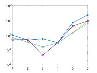
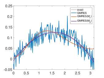
(c)	(d)
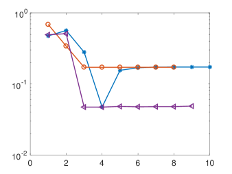
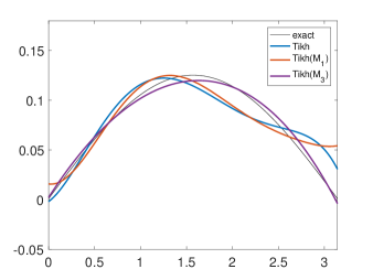
(e)	(f)

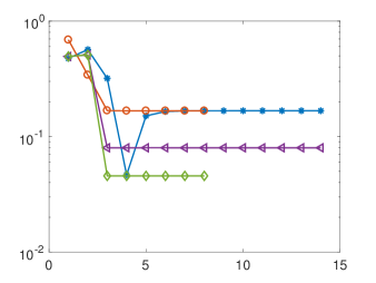
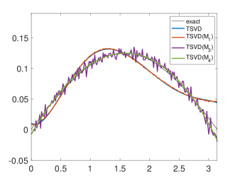
Fig. 1: Test problem baart, with $m=200$ and $\|\mathbf{e}\|/\|\mathbf{b}\|=10^{-2}$. (a) Relative error history, without any additional regularization and $k_{\rm P}=9$. (b) Best approximations, without any additional regularization and $k_{\rm P}=9$. (c) Relative error history, with Arnoldi–Tikhonov and $k_{\rm P}=9$. (d) Approximations for $k=6$, with Arnoldi–Tikhonov and $k_{\rm P}=9$. (e) Relative error history, with Arnoldi-TSVD and $k_{\rm P}=39$. (f) Approximations for $k=9$, with Arnoldi-TSVD and $k_{\rm P}=39$.

heat. We consider a discretization of the inverse heat equation formulated as a Volterra integral equation of the first kind; this problem can be regarded as numerically rank-deficient, with numerical rank equal to 195. According to the analysis in [33], GMRES does not converge to the minimum norm solution of (1) for this problem, as the null spaces of $A$ and $A^{T}$ are different. For this test problem, considering the preconditioned methods described in Section 5, with some of the preconditioners derived in Section 4, can make a dramatic difference. When applying stopping rule (52) to set the number of Arnoldi iterations defining the preconditioners, we get $k_{\rm P}=23$; also for this problem, stopping rule (51) prescribes a similar $k_{\rm P}$. We report the behavior of relevant quantities used to set $k_{\rm P}$ in the bottom frames of Figure 3. In the left frames of Figure 2 we report the relative error history when different preconditioners (also defined with respect to different parameters $k_{\rm P}$) and different solvers are considered. In all these graphs, the unpreconditioned Arnoldi–Tikhonov and Arnoldi-TSVD solutions diverge, with the best approximations being the ones recovered during the first iteration, i.e., the ones belonging to $\textrm{span}\{\mathbf{b}\}$. The approximate solutions computed using the preconditioners (38)-(45) with $k_{\rm P}=23$ do not look much improved; indeed, while the ones obtained with $M_{1}$ and $M_{2}$ do not degenerate as quickly, the ones obtained with $M_{3}$ and $M_{4}$ are even worse than the unpreconditioned ones. However, if the maximum allowed value of $k_{\rm P}$ (i.e., $k_{\rm P}=60$) is chosen, the gain of using a preconditioned approach is evident. While the regularizing preconditioners $M_{3}$ and $M_{4}$ still perform very poorly, the preconditioners $M_{1}$ and $M_{2}$, which seek to make the matrix $AM$ Hermitian positive semidefinite by incorporating an approximate regularized version of $A^{T}$, allow us to reconstruct a solution, whose quality is close to the one achieved with LSQR. The right frames of Figure 2 display the history of the corresponding relative residuals (or discrepancies). We can clearly see that the residuals are good indicators of the performance of these methods. Indeed, for $k_{\rm P}=23$ all the residuals (except for the LSQR one) have quite large norm and, in particular, the discrepancy principle (8), (53), (54) is far from being satisfied. For $k_{\rm P}=60$, the preconditioned Arnoldi–Tikhonov method with the preconditioners $M_{1}$ or $M_{2}$ eventually satisfies the discrepancy principle. Also, the approximate solution obtained with $M_{1}$ reproduces the main features of of the exact solution, though some spurious oscillations are present. This is probably due to the tiny value $\mu=1.2287\cdot 10^{-8}$ selected for the regularization parameter according to the discrepancy principle (53); spurious oscillations are likely to be removed if a larger value for $\mu$ is used. The smallest relative errors attained by each iterative method (considering different choices of solvers and preconditioners) are reported in Table 1, where averages over 30 different realizations of the noise in the vector $\mathbf{b}$ are shown.

(a)	(b)
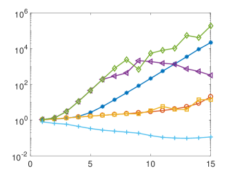
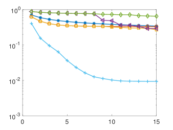
(c)	(d)
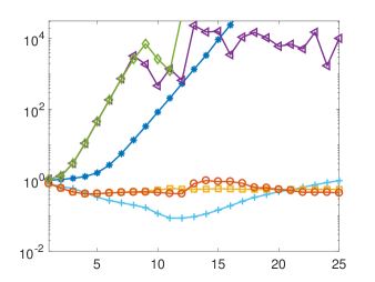
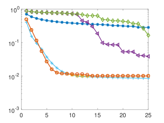
(e)

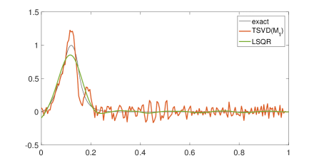
Fig. 2: Test problem heat, with $m=200$ and $\|\mathbf{e}\|/\|\mathbf{b}\|=10^{-2}$. (a) Relative error history, with Arnoldi-TSVD and $k_{\rm P}=23$. (b) Relative residual history, with Arnoldi-TSVD and $k_{\rm P}=23$. (c) Relative error history, with Arnoldi–Tikhonov and $k_{\rm P}=60$. (d) Relative residual history, with Arnoldi–Tikhonov and $k_{\rm P}=60$. (e) Best approximations, with Arnoldi–Tikhonov and $k_{\rm P}=60$.

baart, $h_{i+1,i}$	baart, $p_{\sigma}^{(i)}$
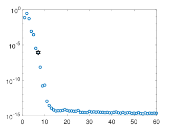
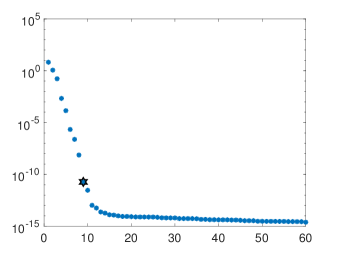
heat, $h_{i+1,i}$	heat, $p_{\sigma}^{(i)}$

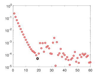
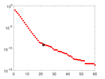
Fig. 3: Illustration of the stopping criteria (51) and (52) for the test problems baart (top row) and heat (bottom row). In the left column, the values of the subdiagonal entries $h_{i+1,i}$ of the Hessenberg matrix $H_{k+1,k}$ are plotted against $i$ ($i=1,\dots,k$). In the right column, the products $p_{\sigma}^{(i)}:=\sigma_{1}^{(i)}\sigma_{i+1}^{(i+1)}$ of the extremal singular values of $H_{i+1,i}$ are plotted against $i$.

Table 1: Average values of the best relative errors over 30 runs of the test problems in the first set of experiments, with $\|\mathbf{e}\|/\|\mathbf{b}\|=10^{-2}$. The smaller parameter $k_{\rm P}$ satisfies, on average, the stopping rule (52); the larger parameter $k_{\rm P}$ is obtained adding 30 to the smaller parameter $k_{\rm P}$.

	baart
	TSVD		Tikh		none
	$k_{\rm P}=9$	$k_{\rm P}=39$	$k_{\rm P}=9$	$k_{\rm P}=39$	$k_{\rm P}=9$	$k_{\rm P}=39$
–	4.7202e-02	4.7202e-02	6.7530e-02	6.7530e-02	3.0950e-01	3.0950e-01
$M_{1}$	2.2148e-02	1.6744e-01	2.4002e-02	1.7926e-01	1.8452e-02	1.5647e-01
$M_{2}$	1.6689e-01	1.2429e-01	1.7733e-01	1.3091e-01	1.5838e-01	1.2517e-01
$M_{3}$	4.5578e-02	6.1255e-02	6.6982e-02	6.7486e-02	4.5029e-02	6.1259e-02
$M_{4}$	1.7025e-02	4.5678e-02	2.4297e-02	6.8386e-02	1.7027e-02	4.1604e-02
LSQR	1.5787e-01	1.5787e-01	1.5787e-01	1.5787e-01	1.5787e-01	1.5787e-01
	heat
	TSVD		Tikh		none
	$k_{\rm P}=20$	$k_{\rm P}=50$	$k_{\rm P}=20$	$k_{\rm P}=50$	$k_{\rm P}=20$	$k_{\rm P}=50$
–	6.5870e-01	6.5870e-01	5.6767e-01	5.6767e-01	1.0584e+00	1.0584e+00
$M_{1}$	1.0296e+00	3.6071e-01	1.0296e+00	3.6173e-01	1.0296e+00	3.6136e-01
$M_{2}$	1.0296e+00	3.6390e-01	1.0119e+00	3.0444e-01	1.0296e+00	3.6390e-01
$M_{3}$	1.0747e+00	1.0747e+00	1.0747e+00	1.0747e+00	1.0747e+00	1.0747e+00
$M_{4}$	1.0747e+00	1.0747e+00	1.0747e+00	1.0375e+00	1.0747e+00	1.0747e+00
LSQR	9.2105e-02	9.2105e-02	9.2105e-02	9.2105e-02	9.2105e-02	9.2105e-02

Second set of experiments

We consider 2D image restoration problems, where the available images are affected by a spatially invariant blur and Gaussian white noise. In this setting, given a point-spread function (PSF) that describes how a single pixel is deformed, a blurring process is modeled as a 2D convolution of the PSF and an exact discrete finite image $X_{\rm exact}\in{\mathbb{R}}^{n\times n}$. Here and in the following, a PSF is represented as a 2D image. A 2D image restoration problem can be expressed as a linear system of equations (1), where the 1D array $\mathbf{b}$ is obtained by stacking the columns of the 2D blurred and noisy image (so that $m=n^{2}$), and the square matrix $A$ incorporates the convolution process together with some given boundary conditions. Our experiments consider two different gray scale test images, two different PSFs, and reflective boundary conditions; the sharp images are artificially blurred, and noise of several levels is added. Matrix-vector products are computed efficiently by using the routines in Restore Tools [40]. The maximum allowed number of Arnoldi iterations in Algorithm 1 is $k=100$, and $k_{\rm P}$ is set according to (52).

Anisotropic motion blur. For this experiment, a geometric test image of size $64\times 64$ pixels is taken as sharp image. It is displayed, together with a PSF modeling motion in two orthogonal directions, and the available corrupted data (with noise level $\|\mathbf{e}\|/\|\mathbf{b}\|=2\cdot 10^{-2}$), in the top frames of Figure 5. GMRES and right-preconditioned GMRES with preconditioners $C_{1}$, $C_{2}$, and $C_{3}$ are considered. The preconditioners $M_{i}$, $i=1,\dots,4$, do not perform well in this case, even when the maximum number of Arnoldi steps $k_{\rm P}=100=k$ is performed; this is probably due to the fact that the PSF is quite unsymmetric. Figure 4 displays the history of the relative reconstruction errors for these solvers. The most effective preconditioner for this problem is $C_{2}$. Moreover, both $C_{1}$ and $C_{2}$ require only a few iterations to compute an accurate solution and exhibit a quite stable behavior afterwards: for this reason we do not consider the Arnoldi–Tikhonov and Arnoldi-TSVD methods for this test problem.

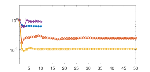
Fig. 4: Image deblurring problem with anisotropic motion blur. Relative error history of GMRES and right-preconditioned GMRES methods (with preconditioners $C_{1}$, $C_{2}$, and $C_{3}$). The GMRES and GMRES($C_{3}$) curves are truncated because severe “semi-convergence” occurs.

Figure 5 shows the best restorations achieved by each method; relative errors and the corresponding number of iterations are displayed in the caption.

exact	PSF	corrupted
GMRES	GMRES($C_{1}$)	GMRES($C_{2}$)

Fig. 5: Image deblurring problem with anisotropic motion blur. The upper row displays the test data. The lower row do spays the best reconstructions obtained by: GMRES method ($6.0804e-01$, $k=13$); GMRES($C_{1}$) method ($1.6452e-01$, $k=2$); GMRES($C_{2}$) method ($8.8234e-02$, $k=3$); GMRES($C_{3}$) method ($6.0316e-01$, $k=3$).

Isotropic motion blur. The test data for this experiment are displayed in Figure 6. We consider a $17\times 17$ PSF modeling diagonal motion blur. The noise level is $5\cdot 10^{-3}$. Figure 7 shows the best restorations achieved by each method; relative errors and the corresponding number of iterations are displayed in the caption.

exact	PSF	corrupted

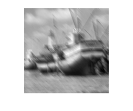
Fig. 6: From left to right: exact image; blow-up ($600\%$) of the diagonal motion PSF; blurred and noisy available image, with $\|\mathbf{e}\|/\|\mathbf{b}\|=5\cdot 10^{-3}$.

TSVD	TSVD($M_{1}$)	TSVD($M_{3}$)

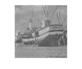
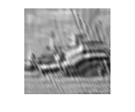
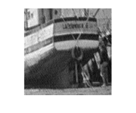
Fig. 7: The lower row displays blow-ups ($200\%$) of the restored images in the upper row. From left to right: unpreconditioned Arnoldi-TSVD method ($1.0481e-01$, $k=26$); TSVD($M_{1}$) method ($1.0081e-01$, $k_{\rm P}=50$, $k=7$); TSVD($M_{3}$) method ($2.5948e-01$, $k_{\rm P}=50$, $k=35$).

All the methods carry out more iterations than in the previous example, due to the smaller amount of noise in the present example. Visual inspection of the images in Figure 7 shows that the unpreconditioned Arnoldi-TSVD solution to bear some motion artifacts, as the restored image displays some shifts in the diagonal directions, i.e., in the direction of the motion blur. These spurious effects are not so pronounced in the TSVD($M_{1}$) restoration, as the preconditioner (38) makes the problem more symmetric. The reconstruction produced by TSVD($M_{3}$) is noticeably worse; indeed, the preconditioner (43) merely approximates a regularized inverse of $A$, and this is not desirable when applying the Arnoldi algorithm to a very unsymmetric blur. The results obtained when applying the Arnoldi–Tikhonov methods are very similar to the ones obtained with the Arnoldi-TSVD methods. We therefore do not show the former.

7 Conclusions

This paper presents an analysis of the GMRES method and the Arnoldi algorithm with applications to the regularization of large-scale linear ill-posed problems. Theoretical properties that involve the distance of the original coefficient matrix to classes of generalized Hermitian matrices are derived. Novel preconditioners based on matrices stemming from the standard Arnoldi decomposition are introduced, and the resulting right-preconditioned linear systems are solved with methods based on the preconditioned Arnoldi algorithm, or the new preconditioned Arnoldi–Tikhonov and Arnoldi-TSVD methods. Numerical results on a variety of test problems clearly show the benefits of applying the new preconditioning techniques.

References

- [1] M. L. Baart, The use of auto-correlation for pseudo-rank determination in noisy ill-conditioned least-squares problems, IMA J. Numer. Anal., 2 (1982), pp. 241–247.
- [2] Å. Björck, Numerical Methods in Matrix Computation, Springer, New York, 2015.
- [3] P. N. Brown and H. F. Walker, GMRES on (nearly) singular systems, SIAM J. Matrix Anal. Appl., 18 (1997), pp. 37–51.
- [4] D. Calvetti, B. Lewis, and L. Reichel, Restoration of images with spatially variant blur by the GMRES method, in Advanced Signal Processing Algorithms, Architectures, and Implementations X, ed. F. T. Luk, Proceedings of the Society of Photo-Optical Instrumentation Engineers (SPIE), vol. 4116, The International Society for Optical Engineering, Bellingham, WA, 2000, pp. 364–374.
- [5] D. Calvetti, B. Lewis, and L. Reichel, On the choice of subspace for iterative methods for linear discrete ill-posed problems, Int. J. Appl. Math. Comput. Sci., 11 (2001), pp. 1069–1092.
- [6] D. Calvetti, B. Lewis, and L. Reichel, Krylov subspace iterative methods for nonsymmetric discrete ill-posed problems in image restoration, in Advanced Signal Processing Algorithms, Architectures, and Implementations XI, ed. F. T. Luk, Proceedings of the Society of Photo-Optical Instrumentation Engineers (SPIE), vol. 4474, The International Society for Optical Engineering, Bellingham, WA, 2001, pp. 224–233.
- [7] D. Calvetti, B. Lewis, and L. Reichel, On the regularizing properties of the GMRES method, Numer. Math., 91 (2002), pp. 605–625.
- [8] D. Calvetti, B. Lewis, and L. Reichel, GMRES, L-curves, and discrete ill-posed problems, BIT, 42 (2002), pp. 44–65.
- [9] D. Calvetti, S. Morigi, L. Reichel, and F. Sgallari, Tikhonov regularization and the L-curve for large discrete ill-posed problems, J. Comput. Appl. Math., 123 (2000), pp. 423–446.
- [10] D. Calvetti and L. Reichel, Tikhonov regularization of large linear problems, BIT, 43 (2003), pp. 263–283.
- [11] D. Calvetti, L. Reichel, and A. Shuibi, Invertible smoothing preconditioners for linear discrete ill-posed problems, Appl. Numer. Math., 54 (2005), pp. 135–149.
- [12] R. H.-F. Chan and X.-Q. Jin, An Introduction to Iterative Toeplitz Solvers, SIAM, Philadelphia, 2007.
- [13] T. F. Chan, An optimal circulant preconditioner for Toeplitz systems, SIAM J. Sci. Statist. Comput., 9 (1988), pp. 766–771.
- [14] T. F. Chan and K. R. Jackson, Nonlinearly preconditioned Krylov subspace methods for discrete Newton algorithms, SIAM J. Sci. Statist. Comput., 5 (1984), pp. 533–542.
- [15] P. J. Davis, Circulant Matrices, 2nd ed., Chelsea, New York, 1994.
- [16] M. Donatelli, D. Martin, and L. Reichel, Arnoldi methods for image deblurring with anti-reflective boundary conditions, Appl. Math. Comput., 253 (2015), pp. 135–150.
- [17] K. Du, J. Duintjer Tebbens, and G. Meurant, Any admissible harmonic Ritz value set is possible for GMRES, Electron. Trans. Numer. Anal., 47 (2017), pp. 37–56.
- [18] L. Dykes, S. Noschese, and L. Reichel, Circulant preconditioners for discrete ill-posed Toeplitz systems, Numer. Algorithms, 75 (2017), pp. 477–490.
- [19] L. Dykes and L. Reichel, A family of range restricted iterative methods for linear discrete ill-posed problems, Dolomites Research Notes on Approximation, 6 (2013), pp. 27–36.
- [20] S. C. Eisenstat, Equivalence of Krylov subspace methods for skew-symmetric linear systems, arXiv:1512.00311, 2015.
- [21] H. W. Engl, M. Hanke, and A. Neubauer, Regularization of Inverse Problems, Kluwer, Dordrecht, 1996.
- [22] S. Gazzola, P. Novati, and M. R. Russo, Embedded techniques for choosing the parameter in Tikhonov regularization, Numer. Linear Algebra Appl., 21 (2014), pp. 796–812.
- [23] S. Gazzola, P. Novati, and M. R. Russo, On Krylov projection methods and Tikhonov regularization, Electron. Trans. Numer. Anal., 44 (2015), pp. 83–123.
- [24] L. Greengard and V. Rokhlin, A new version of the fast multipole method for the Laplace equation in three dimensions, Acta Numer., 6 (1997), pp. 229–269.
- [25] M. Hanke, Conjugate Gradient Type Methods for Ill-Posed Problems, Longman, Harlow, 1995.
- [26] M. Hanke, J. Nagy, and R. Plemmons, Preconditioned iterative regularization for ill-posed problems, in L. Reichel, A. Ruttan, and R. S. Varga, eds., Numerical Linear Algebra, de Gruyter, Berlin, 1993, pp. 141–163.
- [27] P. C. Hansen, Regularization Tools version 4.0 for Matlab 7.3, Numer. Algorithms, 46 (2007), pp. 189–194.
- [28] P. C. Hansen, Rank-Deficient and Discrete Ill-Posed Problems, SIAM, Philadelphia, 1998.
- [29] P. C. Hansen and T. K. Jensen, Smoothing-norm preconditioning for regularizing minimum-residual methods, SIAM J. Matrix Anal., 29 (2006), pp. 1–14.
- [30] P. C. Hansen and T. K. Jensen, Noise propagation in regularizing iterations for image deblurring, Electron. Trans. Numer. Anal., 31 (2008), pp. 204–220.
- [31] N. J. Higham, Computing a nearest symmetric positive semidefinite matrix, Linear Algebra Appl., 103 (1988), pp. 103–118.
- [32] T. Huckle, The Arnoldi method for normal matrices, SIAM J. Matrix Anal. Appl., 15 (1994), pp. 479–489.
- [33] T. K. Jensen and P. C. Hansen, Iterative regularization with minimal residual methods, BIT, 47 (2007), pp. 103–120.
- [34] S. Kindermann, Convergence analysis of minimization-based noise level-free parameter choice rules for linear ill-posed problems, Electron. Trans. Numer. Anal., 38 (2011), pp. 233–257.
- [35] B. Lewis and L. Reichel, Arnoldi–Tikhonov regularization methods, J. Comput. Appl. Math., 226 (2009), pp. 92–102.
- [36] D. Loghin, D. Ruiz, and A. Touhami, Adaptive preconditioners for nonlinear systems of equations, J. Comput. Appl. Math., 189 (2006), pp. 362–374.
- [37] I. Moret, A note on the superlinear convergence of GMRES, SIAM J. Numer. Anal., 34 (1997), pp. 513–516.
- [38] N. M. Nachtigal, S. C. Reddy, and L. N. Trefethen, How fast are nonsymmetric matrix iterations?, SIAM J. Matrix Anal. Appl., 13 (1992), pp. 778–795.
- [39] N. M. Nachtigal, L. Reichel, and L. N. Trefethen, A hybrid GMRES algorithm for nonsymmetric linear systems, SIAM J. Matrix Anal. Appl., 13 (1992), pp. 796–825.
- [40] J. G. Nagy, K. M. Palmer, and L. Perrone, Iterative methods for image deblurring: a Matlab object oriented approach, Numer. Algorithms, 36 (2004), pp. 73–93.
- [41] A. Neuman, L. Reichel, and H. Sadok, Implementations of range restricted iterative methods for linear discrete ill-posed problems, Linear Algebra Appl., 436 (2012), pp. 3974–3990.
- [42] M. K. Ng, Iterative Methods for Toeplitz Systems, Oxford University Press, Oxford, 2004.
- [43] S. Noschese, L. Pasquini, and L. Reichel, The structured distance to normality of an irreducibel real tridiagonal matrix, Electron. Trans. Numer. Anal., 28 (2007), pp. 65–77.
- [44] S. Noschese, L. Pasquini, and L. Reichel, Tridiagonal Toeplitz matrices: properties and novel applications, Numer. Linear Algebra Appl., 20 (2013), pp. 302–326.
- [45] S. Noschese and L. Reichel, The structured distance to normality of Toeplitz matrices with application to preconditioning, Numer. Linear Algebra Appl., 18 (2011), pp. 429–447.
- [46] S. Noschese and L. Reichel, A modified TSVD method for discrete ill-posed problems, Numer. Linear Algebra Appl., 21 (2014), pp. 813–822.
- [47] S. Noschese and L. Reichel, A note on superoptimal generalized circulant preconditioners, Appl. Numer. Math., 75 (2014), pp. 188–195.
- [48] P. Novati, Some properties of the Arnoldi based methods for linear ill-posed problems, SIAM J. Numer. Anal. 55 (2017), pp. 1437–1455.
- [49] P. Novati and M. R. Russo, A GCV based Arnoldi–Tikhonov regularization method, BIT, 54 (2014), pp. 501–521.
- [50] C. C. Paige and M. A. Saunders, Solution of sparse indefinite systems of linear equations, SIAM J. Numer. Anal., 12 (1975), pp. 617–629.
- [51] C. C. Paige and M. A. Saunders, LSQR: An algorithm for sparse linear equations and sparse least squares, ACM Trans. Math. Software, 8 (1982), pp. 43–71.
- [52] D. L. Phillips, A technique for the numerical solution of certain integral equations of the first kind, J. ACM, 9 (1962), pp. 84–97.
- [53] L. Reichel and G. Rodriguez, Old and new parameter choice rules for discrete ill-posed problems, Numer. Algorithms, 63 (2013), pp. 65–87.
- [54] L. Reichel and Q. Ye, Breakdown-free GMRES for singular systems, SIAM J. Matrix Anal. Appl., 26 (2005), pp. 1001–1021.
- [55] L. Reichel and Q. Ye, Simple square smoothing regularization operators, Electron. Trans. Numer. Anal., 33 (2009), pp. 63–83.
- [56] J. R. Ringrose, Compact Non-Self-Adjoint Operators, Van Nostrand Reinhold, London, 1971.
- [57] Y. Saad, Iterative Methods for Sparse Linear Systems, 2nd ed., SIAM, Philadelphia, 2003.
- [58] Y. Saad and M. H. Schultz, GMRES: a generalized minimal residual method for solving nonsymmetric linear systems, SIAM J. Sci. Stat. Comput., 7 (1986), pp. 856–869.
- [59] C. B. Shaw, Jr., Improvements of the resolution of an instrument by numerical solution of an integral equation, J. Math. Anal. Appl., 37 (1972), pp. 83–112.
- [60] V. V. Strela and E. E. Tyrtyshnikov, Which circulant preconditioner is better?, Math. Comp., 65 (1996), pp. 137–150.
- [61] E. E. Tyrtyshnikov, Optimal and superoptimal circulant preconditioners, SIAM J. Matrix Anal. Appl., 13 (1992), pp. 459–473.