HitNet: a neural network with capsules embedded in a Hit-or-Miss layer, extended with hybrid data augmentation and ghost capsules

Abstract

Neural networks designed for the task of classification have become a commodity in recent years. Many works target the development of better networks, which results in a complexification of their architectures with more layers, multiple sub-networks, or even the combination of multiple classifiers. In this paper, we show how to redesign a simple network to reach excellent performances, which are better than the results reproduced with CapsNet on several datasets, by replacing a layer with a Hit-or-Miss layer. This layer contains activated vectors, called capsules, that we train to hit or miss a central capsule by tailoring a specific centripetal loss function. We also show how our network, named HitNet, is capable of synthesizing a representative sample of the images of a given class by including a reconstruction network. This possibility allows to develop a data augmentation step combining information from the data space and the feature space, resulting in a hybrid data augmentation process. In addition, we introduce the possibility for HitNet, to adopt an alternative to the true target when needed by using the new concept of ghost capsules, which is used here to detect potentially mislabeled images in the training data.

1 Introduction

Figure 1: Graphical representation of the structure of our new network, named HitNet. Our contributions are highlighted in red, and comprise a new Hit-or-Miss layer, a centripetal loss, prototypes that can be built with the decoder, and ghost capsules that can be embedded in the HoM layer. Source code is available at http://www.telecom.ulg.ac.be/hitnethttp://www.telecom.ulg.ac.be/hitnet.

Convolutional neural networks (CNNs) have become an omnipresent tool for image classification and have been revolutionizing the field of computer vision for the last few years. With the emergence of complex tasks such as ImageNet classification [4], the networks have grown bigger and deeper while regularly featuring new layers and other extensions. However, CNNs are not intrinsically viewpoint-invariant, meaning that the spatial relations between different features are generally not preserved when using CNNs. Therefore, some models were designed in the spirit of increasing their representational power by encapsulating information in activated vectors called capsules, a notion introduced by Hinton in [6].

Recent advances on capsules are presented in [22], in which Sabour et al. mainly focus on MNIST digits classification [11]. For that purpose, they develop CapsNet, a CNN that shows major changes compared to conventional CNNs. As described in [22], “a capsule is a group of neurons whose activity vector represents the instantiation parameters of a specific type of entity such as an object or an object part.” Hence, the concept of capsule somehow adds a (geometrical) dimension to the “capsuled” layers, which is meant to contain richer information about the features captured by the network than in conventional feature maps. The transfer of information from the capsules of a layer to the capsules of the next layer is learned through a dynamic routing mechanism [7, 22]. The length of the capsules of the last layer, called DigitCaps, is used to produce a prediction vector whose entries are in the $[0,1]$ range thanks to an orientation-preserving squashing activation applied beforehand to each capsule, and which encodes the likelihood of the existence of each digit on the input image. This prediction vector is evaluated through a “margin loss” that displays similarities with the squared Hinge loss. In an encoder-decoder spirit, the capsules of DigitCaps can be fed to a decoder sub-network that aims at reconstructing the initial image, which confers the capsules a natural interpretation of the features that they encoded.State-of-the-art results are reported by Sabour et al. in [22] on MNIST dataset. Other experiments carried out on affNIST [26], multiMNIST [22], SVHN [18], smallNORB [12] and CIFAR10 [9] (with an ensemble of 7 networks) show promising results as well. Unfortunately, current implementations of CapsNet with dynamic routing are considerably slower than conventionnal CNNs, which is a major drawback of this process.

Since the publication of [22], several works have been conducted to improve CapsNet’s speed and structure ([3, 7, 21, 28]) and to apply it to more complex data ([1, 14, 19]) and various tasks ([16] for localization, [10] for segmentation, [29] for hypernymy detection, [2] for reinforcement learning). However, it appears that all the attempts (e.g. [5, 15, 17, 24]) to reproduce the results provided in [22] failed to reach the performances reported by Sabour et al.

The first part of this work is devoted to the construction of a neural network, named HitNet, that uses the capsule approach only in one layer, called Hit-or-Miss layer (HoM, the counterpart of DigitCaps) and that provides fast and repeatedly better performances than those reported in [5, 15, 17, 24] with CapsNet. We also provide its associated loss, that we call centripetal loss (counterpart of the margin loss).

The strong representational behavior expected from CapsNet allows to perform the joint multi-task of classification and reconstruction. It is thus possible to take advantage of capsules to capture the natural variations of important class-specific features of the training data, as illustrated in [22]. By browsing through the space of features and using the decoder appropriately, it is thus possible to perform data generation and data augmentation. Augmenting the data is recognized as a powerful way to prevent overfitting and increase the ability of the network to generalize to unseen data at test time, which leads to better classification results [20]. This process is often applied entirely either in the data space or in the feature space [30]. As a second part, we present a way of using the capsules of HoM to derive a hybrid data augmentation algorithm that relies on both real data and synthetic feature-based data by introducing the notion of prototype, a class representative learned indirectly by the decoder.

Not only do we use capsules for data-driven applications such as data generation and data augmentation, but we can also use them to define new notions that serve novel purposes. The one that we want to highlight as third part is the possibility to allow HitNet to adopt an alternative choice to the true class when needed, through the notion of ghost capsule that we embed in HoM. More specifically, in this work, we show how to use ghost capsules to analyze the training set and to detect potentially mislabeled training images, which is often eluded in practice despite being of paramount importance.

In short, our contributions are threefold:

1. We develop HitNet, a neural network that uses capsules in a new way through a Hit-or-Miss layer and a centripetal loss, and we demonstrate the superiority of HitNet over the results reproduced by other authors with CapsNet.

2. We derive a hybrid data space and feature space data augmentation process via the capsules of HoM and prototypes.

3. We provide a way for HitNet to identify another plausible class for the training images if necessary with the new notion of ghost capsules. We exemplify this notion by detecting potentially mislabeled training images, or training images that may need two labels.

These contributions are described in that order in Section 2, then tested in Section 3.

2 HitNet: rethinking DigitCaps and beyond

HitNet essentially introduces a new layer, the Hit-or-Miss layer, that is universal enough to be used in many different networks. HitNet as presented hereafter is thus an instance of a shallow network that hosts this HoM layer and illustrates its potential.

2.1 Introducing hits, misses, the centripetal approach, and the Hit-or-Miss layer

In the case of CapsNet, large activated values are expected from the capsule of DigitCaps corresponding to the true class of a given image, similarly to usual networks. From a geometrical perspective in the feature space, this results in a capsule that can be seen as a point that the network is trained to push far from the center of the unit hypersphere, in which it ends up thanks to the squashing activation function. We qualify such an approach as “centrifugal”. In that case, a first possible issue is that one has no control on the part(s) of the sphere that will be targeted by CapsNet, and a second one is that the capsules of two images of the same class might be located far from each other ([23, 32]), which are two debatable behaviors.

To solve these issues, we hypothesize that all the images of a given class share some class-specific features and that this assumption should also manifest through their respective capsules. Hence, given an input image, we impose that HitNet targets the center of the feature space to which the capsule of the true class belongs, so that it corresponds to what we call a hit. The capsules related to the other classes have thus to be sent far from the center of their respective feature spaces, which corresponds to what we call a miss. Our point of view is thus the opposite of Sabour et al.’s; instead, we have a centripetal approach with respect to the true class.

The squashing activation function induces a dependency between the features of a capsule of DigitCaps, in the sense that their values are conditioned by the overall length of the capsule. If one feature of a capsule has a large value, then the squashing prevents the other features of that capsule to take large values as well; alternatively, if the network wishes to activate many features in a capsule, then none of them will be able to have a large value. None of these two cases fit with the perspective of providing strong activations for several representative features as desired in Sabour et al. Besides, the orientation of the capsules, preserved with the squashing activation, is not used explicitly for the classification; preserving the orientation might thus be a superfluous constraint.

Therefore, we replace this squashing activation by a BatchNormalization (BN, [8]) followed by a conventional sigmoid activation function applied element-wise. We obtain a layer composed of capsules as well that we call the Hit-or-Miss (HoM) layer, which is HitNet’s counterpart of DigitCaps. Consequently, all the features obtained in HoM’s capsules can span the $[0,1]$ range and they can reach any value in this interval independently of the other features. The feature spaces in which the capsules of HoM lie are thus unit hypercubes.

Defining the centripetal loss

Given the use of the element-wise sigmoid activation, the centers of the reshaped target spaces are, for each of them, the central capsules $C:(0.5,\,\ldots,\,0.5)$. The $k$-th component of the prediction vector $y_{\text{pred}}$ of HitNet, denoted $y_{\text{pred},\,k}$, is given by the Euclidean distance between the $k$-th capsule of HoM and $C$:

$$y_{\text{pred},\,k}=||\text{HoM}_{k}-C||.$$ (1)

To give a tractable form to the notions of hits, misses, centripetal approach described above and justify HoM’s name, we design a custom centripetal loss function with the following requirements:

1. The loss generated by each capsule of HoM has to be independent of the other capsules. We thus get rid of any probabilistic notion during the training.

2. The capsule of the true class does not generate any loss when belonging to a close isotropic neighborhood of $C$, which defines the hit zone. Outside that neighborhood, it generates a loss increasing with its distance to $C$. The capsules related to the remaining classes generate a loss decreasing with their distance to $C$ inside a wide neighborhood of $C$ and do not generate any loss outside that neighborhood, which is the miss zone. These loss-free zones are imposed to stop penalizing capsules that are already sufficiently close (if associated with the true class) or far (if associated with the other classes) from $C$ in their respective feature space.

3. The gradient of the loss with respect to $y_{\text{pred},\,k}$ cannot go to zero when the corresponding capsule approaches the loss-free zones defined in requirement 2. To guarantee this behavior, we impose a constant gradient around these zones. This is imposed to help the network make hits and misses.

4. For the sake of consistency with requirement 3, we impose piecewise constant gradients with respect to $y_{\text{pred},\,k}$, which thus defines natural bins around $C$, as the rings of archery targets, in which the gradient is constant.

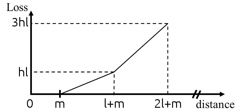
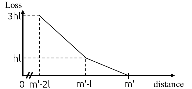
All these elements contribute to define a loss which is a piecewise linear function of the predictions and which is centripetal with respect to the capsule of the true class. We thus call it our centripetal loss. Its derivative with respect to $y_{\text{pred},\,k}$ is a staircase-like function, which goes up when $k$ is the index of the true class (see Figure 2a) and goes down otherwise (see Figure 2b). A generic analytic formula of a function of a variable $x$, whose derivative is an increasing staircase-like function where the steps have length $l$ and height $h$ and vanish on $[0,m]$ is mathematically given by:

$$L_{l,h,m}(x)=H\{x-m\}\,(f+1)\,h\,(x-m-0.5\,f\,l),$$ (2)

where $H\{.\}$ denotes the Heaviside step function and $f=\left\lfloor\frac{x-m}{l}\right\rfloor$ ($\left\lfloor.\right\rfloor$ is the floor function). Hence the loss generated by the capsule of the true class is given by $L_{l,h,m}(y_{\text{pred},\,k})$, where $k$ is the index of the true class. The loss generated by the capsules of the other classes can be directly obtained from Equation 2 as $L_{l^{\prime},h^{\prime},\sqrt{n}/2-m^{\prime}}(\sqrt{n}/2-y_{\text{pred},\,k^{\prime}})$ (for any index $k^{\prime}$ of the other classes) if the steps have length $l^{\prime}$, height $h^{\prime}$, vanish after $m^{\prime}$ and if the capsules have $n$ components. The use of $\sqrt{n}/2$ originates from the fact that the maximal distance between a capsule of HoM and $C$ is given by $\sqrt{n}/2$ and thus the entries of $y_{\text{pred}}$ will always be in the interval $[0,\sqrt{n}/2]$. Consequently, the centripetal loss of a given training image is given by

$$L=\sum_{k=1}^{K}y_{\text{true},\,k}\,L_{l,h,m}(y_{\text{pred},\,k})+\lambda(1-y_{\text{true},\,k})\,L_{l^{\prime},h^{\prime},\sqrt{n}/2-m^{\prime}}(\sqrt{n}/2-y_{\text{pred},\,k})$$ (3)

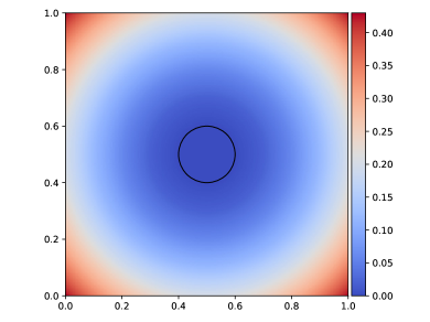
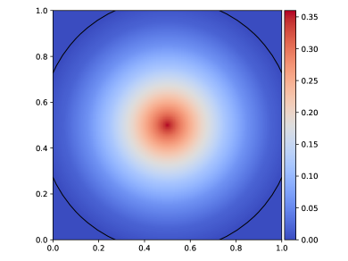
where $K$ is the number of classes, $y_{\text{true},\,k}$ denotes the $k$-th component of the vector $y_{\text{true}}$, and $\lambda$ is a down-weighting factor set as $0.5$ as in [22]. The loss associated with the capsule of the true class and the loss associated with the other capsules are represented in Figure 2 in the case where $n=2$.

(a)

(b)

(c)

(d)

Figure 2: Representation of the centripetal loss given in Equation 2 as function of the distance of the capsule of the true class (a) and of the other classes (b) from $C$. Then, visualization of the centripetal loss in the 2-dimensional case ($n=2$). The loss associated with the capsule of the true class is given by plot (c). The loss-free hit zone is the area within the black circle, with radius $m$. The loss generated by the other capsules is given by plot (d). The loss-free miss zone is the area outside the black circle, with radius $m^{\prime}$.

Architecture of HitNet

Basically, HitNet incorporates a HoM layer built upon feature maps and used in pair with the centripetal loss. In our experiments, we have adopted a shallow structure to obtain these feature maps to highlight the benefits of the HoM layer. HitNet’s complete architecture is displayed in Figure 1. It is composed of the following elements:

1. Two $9\times 9$ (with strides (1,1) then (2,2)) convolutional layers with 256 channels and ReLU activations, to obtain feature maps.

2. A fully connected layer to a $K\times n$ matrix, followed by a BN and an element-wise sigmoid activation, which produces HoM composed of $K$ capsules of size $n$.

3. The Euclidean distance with the central capsule $C:(0.5,\,\ldots,\,0.5)$ is computed for each capsule of HoM, which gives the prediction vector of the model $y_{\text{pred}}$.

4. All the capsules of HoM are masked (set to $0$) except the one related to the true class (to the predicted class at test time), then they are concatenated and sent to a decoder, which produces an output image $X_{\text{rec}}$, that aims at reconstructing the initial image. The decoder consists in two fully connected layers of size $512$ and $1024$ with ReLU activations, and one fully connected layer to a matrix with the same dimensions as the input image, with a sigmoid activation (this is the same decoder as in [22]).

If $X$ is the initial image and $y_{\text{true}}$ its one-hot encoded label, then $y_{\text{true}}$ and $y_{\text{pred}}$ produce a loss $L_{1}$ through the centripetal loss given by Equation 3 while $X$ and $X_{\text{rec}}$ generate a loss $L_{2}$ through the mean squared error. The final composite loss associated with $X$ is given by $L=L_{1}+\alpha\,L_{2}$, where $\alpha$ is set to $0.392$ ([5, 22]). For the classification task, the label predicted by HitNet is the index of the lowest entry of $y_{\text{pred}}$. The hyperparameters involved in $L_{1}$ are chosen as $l=l^{\prime}=0.1$, $h=h^{\prime}=0.2$, $m=0.1$, $m^{\prime}=0.9$, $n=16$ and $\lambda=0.5$ as in [22].

2.2 Beyond HitNet: Prototypes, data generation and hybrid data augmentation

Prototypes

The simultaneous use of HoM and a decoder offers new possibilities in terms of image processing. It is essential to underline that in our centripetal approach, we ensure that all the images of a given class will have all the components of their capsule of that class close to $0.5$. In other words, we regroup these capsules in a convex space around $C$. This central capsule $C$ stands for a fixed point of reference, hence different from a centroid, from which we measure the distance of the capsules of HoM; from the network’s point of view, $C$ stands for a capsule of reference from which we measure deformations. In consequence, we can use $C$ instead of the capsule of a class of HoM, zero out the other capsules and feed the result in the decoder: the reconstructed image will correspond to the image that the network considers as a canonical image of reference for that class, which we call its prototype.

Data generation

After constructing the prototypes, we can slightly deform them to induce variations in the reconstruction without being dependent on any training image, just by feeding the decoder with a zeroed out HoM plus one capsule in a neighborhood of $C$. This allows to identify what the features of HoM represent. For the same purpose, Sabour et al. need to rely on a training image because the centrifugal approach does not directly allows to build prototypes. In our case, it is even possible to compute an approximate range in which the components can be tweaked. If a sufficient amount of training data is available, we can expect the individual features of the capsules of the true classes to be approximately Gaussian distributed with mean $0.5$ and standard deviation $m/\sqrt{n}$, thus the $[0.5-2m/\sqrt{n},0.5+2m/\sqrt{n}]$ interval should provide a satisfying overview of the physical interpretation embodied in a given feature of HoM. The approximate knowledge of the distributions also enables us to perform data generation, by sampling for instance a Gaussian vector of size $n$, with mean $0.5$ and standard deviation $m/\sqrt{n}$ , inserting it as a capsule in HoM, zeroing out the other capsules and feeding the result in the decoder.

Hybrid data augmentation

The capsules of HoM only capture the important features that allow the network to identify the class of the images and to perform an approximate reconstruction via the decoder. This implies that the images produced by the decoder are not detailed enough to look realistic. The details are lost in the process; generating them back is hard. It is easier to use already existing details, i.e. those of images of the training set. We can thus set up a hybrid feature-based and data-based data augmentation process:

• Take a training image $X$ and feed it to a trained HitNet network.

• Extract its HoM and modify the capsule corresponding to the class of $X$.

• Reconstruct the image obtained from the initial capsule, $X_{\text{rec}}$, and from the modified one, $X_{\text{mod}}$.

• The details of $X$ are contained in $X-X_{\text{rec}}$. Thus the new (detailed) image is $X_{\text{mod}}+X-X_{\text{rec}}$. Clip the values to ensure that the resulting image has values in the appropriate range (e.g. [0,1]).

2.3 Beyond HitNet: Ghost capsules

One of the main assets of HitNet is the flexibility in the use of the HoM layer. It can be easily exploited to perform different tasks other than classification. In order to show an additional possibility of HitNet, we develop the notion of ghost capsules, that can be integrated within the network. The use of ghost capsules allows the network, for each training sample, to zero-out the loss associated with a capsule related to a class that the network considers as a reasonable prediction and that is different from the true class. Several situations can benefit from this process. For example, it can be used to assess the quality of the training set through the detection of potentially mislabeled images in that set. Detecting them is an important aspect since mislabeled training data pollute the whole training by forcing the network to learn unnatural features, or even mistakes; this constrains the network to memorize outliers in dedicated neurons.

Definition of “ghost capsule”

In order to give the network the capacity to allow an alternative to the labels provided, we introduce the notion of “ghost capsule”, which is associated with every image of the training set. The key idea is the following: during the training phase, for each image, instead of forcing the network to produce one capsule that makes a hit and $K-1$ capsules that make misses, we demand one hit for the capsule of the true class and $K-2$ misses for as many capsules of the other classes; the remaining capsule is the so-called “ghost capsule”, denoted by GC hereafter. By “capsule of the true class” of an image, we mean the capsule associated with the class corresponding to the label provided by the annotator with the image. The GC is the capsule of the HoM layer which is the closest to $C$ among the $K-1$ capsules not corresponding to the true class. The loss associated with the GC is zeroed out, hence the GC is not forced to make a hit nor a miss, and it is not involved in the update of the weights from one batch to the next; it is essentially invisible to the loss in the back-propagation, hence its name.

From an implementation point of view, training HitNet with a GC per image is similar to training it without GC; only the centripetal loss needs to be adjusted. Given a training image, its one-hot encoded label $y_{\text{true}}$ and the output vector of the network $y_{\text{pred}}$, the centripetal loss initially defined by Equation 3 formally becomes

$$L_{\text{ghost}}=\sum_{k=1}^{K}y_{\text{true},\,k}\,L_{l,h,m}(y_{\text{pred},\,k})+\lambda(1-{\color[rgb]{1,0,0}\tilde{y}_{\text{true},\,k}})\,L_{l^{\prime},h^{\prime},\sqrt{n}/2-m^{\prime}}(\sqrt{n}/2-y_{\text{pred},\,k}),$$ (4)

where ${\color[rgb]{1,0,0}\tilde{y}_{\text{true},\,k}}=1$ if $k$ is the true class index or the GC class index, and ${\color[rgb]{1,0,0}\tilde{y}_{\text{true},\,k}}=0$ otherwise.

Two important characteristics are thus associated with a GC: its class, which is always one of the $K-1$ classes not corresponding to the true class of the sample, and its distance with $C$. The GC class of an image is obtained in a deterministic way, it is not a Dropout ([25]) nor a learned Dropout variant (as e.g. [13]). Besides, this class is likely to change from one epoch to the next in the early stages of the training, until the network decides what choice is the best. Ideally, a GC will make a hit when its class is a plausible alternative to the true class or if the image deserves an extra label, and will make a miss otherwise. The evolution of a GC during the training is dictated by the overall evolution of the network.

Subsequently, in the situations described above, at the end of the training, mislabeled or confusing images should actually display two hits: one hit for the capsule corresponding to the true class since the network was forced to make that hit, and one hit for the capsule corresponding to the other plausible class since the network was not told to push this capsule towards the miss zone and since the image displays the features needed to identify this alternate class. Looking at the images with a GC in the hit zone at the end of the training allows to detect the images for which the network suspects an error in the label, or which images possibly deserve two labels.

3 Experiments and results

In this section, we present some experiments and the results obtained with HitNet. The structure of the section mirrors that of Section 2, i.e. it is divided in three parts, which directly correspond to the three parts of Section 2: (1) general performances of HitNet, (2) use of the decoder, and (3) use of ghost capsules.

3.1 Classification results of HitNet

Hereafter, we report the results obtained with HitNet. First, we compare the performances of HitNet on MNIST classification task with baseline models to show that HitNet produces repeatedly close to state-of-the-art performances. Then, we compare the performances of HitNet with reproduced experiments with CapsNet on several datasets.

Description of the networks used for comparison

We compare the performances of HitNet to three other networks for the MNIST digits classification task. For the sake of a fair comparison, a structure similar to HitNet is used as much as possible for these networks. First, they are made of two $9\times 9$ convolutional layers with 256 channels (with strides (1,1) then (2,2)) and ReLU activations as for HitNet. Then, the first network is N1:

• N1 (baseline model, conventional CNN) has a fully connected layer to a vector of dimension $10$, then BN and Softmax activation, and is evaluated with the usual categorical cross-entropy loss. No decoder is used.

The two other networks, noted N2 and N2b, have a fully connected layer to a $10\times 16$ matrix, followed by a BN layer as N1 and HitNet, then

• N2 (CapsNet-like model) has a squashing activation. The Euclidean distance with $O:(0,\,\ldots,\,0)$ is computed for each capsule, which gives the output vector of the model $y_{\text{pred}}$. The margin loss (centrifugal) of [22] is used;

• N2b has a sigmoid activation. The Euclidean distance with $C:(0.5,\,\ldots,\,0.5)$ is computed for each capsule, which gives the output vector of the model $y_{\text{pred}}$. The margin loss (centrifugal) of [22] is used.

Let us recall that, compared to N2 and N2b, HitNet has a sigmoid activation, which produces the capsules of HoM. The $L^{2}$ distance with $C:(0.5,\,\ldots,\,0.5)$ is computed for each capsule, which gives the output vector of the model $y_{\text{pred}}$, and the centripetal loss given by Equation 3 is used. Network N2b is tested to show the benefits of the centripetal approach of HitNet over the centrifugal one, regardless of the squashing or sigmoid activations. Also, during the training phase, the decoder used in HitNet is also used with N2 and N2b.

Classification results on MNIST

Each network is trained $20$ times during $250$ epochs with the Adam optimizer with a constant learning rate of $0.001$, with batches of $128$ images. The images of a batch are randomly shifted of up to $2$ pixels in each direction (left, right, top, bottom) with zero padding as in [22]. The metrics presented here for a given network are the average metrics over the $20$ runs of that network calculated on the MNIST test set. The learning rate is kept constant to remove its possible influence on the results, which may differ from one network structure to another. Besides, this lead us to evaluate the “natural” convergence of the networks since the convergence is not forced by a decreasing learning rate mechanism. To our knowledge, this practice is not common but should be used to properly analyze the natural convergence of a network.

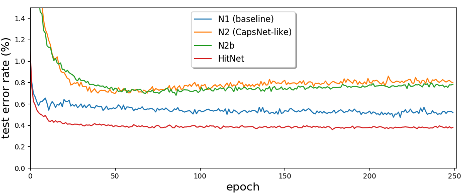
The results throughout the epochs are plotted in Figure 3. The error rates of the four models are reported in Table 1 and, as it can also be seen in Figure 3, they clearly indicate that the centripetal approach of HitNet is better suited than a centrifugal approach, regardless of the activation used. This observation is confirmed if the squashing function is used in HitNet, in which case a test error rate of about $0.40\%$ is obtained.

In Table 1, the column “Standard deviation (Std)” represents the variability that is obtained in the error rate among the $20$ runs of a given network. The column “Irregularity” relates to the average (over the $20$ runs) of the standard deviation of the last $100$ error rates recorded for each run. A low irregularity represents a more “natural” convergence of the runs of a given network since it measures the variability of the error rate within a run. This indicator makes sense in the context of a constant learning rate and no overfitting, as observed with HitNet.

These two metrics both indicate superior performances when using HitNet, in the sense that there is an intrinsically better natural convergence associated with the centripetal approach (lower irregularity) and more consistent results between the runs of a same model (lower standard deviation). Let us note that all the runs of HitNet converged and no overfitting is observed. The question of the convergence is not studied in [22] and the network is stopped before it is observed diverging in [17].

Then, we run the same experiments but with a decreasing learning rate, to see how the results are impacted when the convergence is forced. The learning rate is multiplied by a factor $0.95$ at the end of each epoch. As a result, the networks stabilize more easily around a local minimum of the loss function, improving their overall performances. It can be noted that HitNet is less impacted, which indicates that HitNet converges to similar states with or without decreasing learning rate. The conclusions are the same as previously: HitNet performs better. Let us note that in this case, the irregularity is not useful anymore. We replace it by the best error rate obtained for a converged run of each type of network.

Figure 3: Evolution of the average test error rate on MNIST over the $20$ runs of each network as a function of the epochs, with a constant learning rate. The superiority of HitNet can be seen. The convergence is also finer in that case, in light of the weaker oscillations from one epoch to the next (lower irregularity).

	Constant learning rate			Decreasing learning rate
Network	Err. rate %	Std ($\times 10^{-2}$)	Irreg. ($\times 10^{-2}$)	Err. rate %	Std ($\times 10^{-2}$)	Best %
Baseline	$0.52$	$0.060$	$0.060$	$0.42$	$0.027$	$0.38$
CapsNet-like	$0.79$	$0.089$	$0.053$	$0.70$	$0.076$	$0.53$
N2b	$0.76$	$0.072$	$0.048$	$0.72$	$0.074$	$0.62$
HitNet	$\mathbf{0.38}$	$\mathbf{0.033}$	$\mathbf{0.025}$	$\mathbf{0.36}$	$\mathbf{0.025}$	$\mathbf{0.32}$

Table 1: Performance metrics on MNIST of the four networks described in the text, showing the superiority of HitNet.

Comparisons with reported results of CapsNet on several datasets

As far as MNIST is concerned, the best test error rate reported in [22] is $0.25\%$, which is obtained with dynamic routing and is an average of 3 runs only. However, to our knowledge, this result has yet to be confirmed, as the best tentative reproductions reach error rates which compare with our results, as shown in Table 2. Let us note that, in [27], authors report a $0.21\%$ test error rate, which is the best performance published so far. Nevertheless, this score is reached with a voting committee of five networks that were trained with random crops, rotation and scaling as data augmentation processes. They achieve $0.63\%$ without the committee and these techniques; if only random crops are allowed (as done here with the shifts of up to 2 pixels), they achieve $0.39\%$. It is important to underline that such implementations report excessively long training times, mainly due to the dynamic routing part. For example, the implementation [5] appears to be about $13$ times slower than HitNet, for comparable performances. Therefore, HitNet produces results consistent with state-of-the art methods on MNIST while being simple, light and fast.

The results obtained with HitNet and those obtained with CapsNet in different sources on Fashion-MNIST, CIFAR10, SVHN, affNIST are also compared in Table 2. For fair comparisons, the architecture of HitNet described in Section 2.1 is left untouched. The results reported are obtained with a constant learning rate and are average error rates on $20$ runs as previously. Some comments about these experiments are given below:

1. Fashion-MNIST: HitNet outperforms reproductions of CapsNet except for [5], but this result is obtained with horizontal flipping as additional data augmentation process.

2. CIFAR10: HitNet outperforms the reproductions of CapsNet. The result provided in [22] is obtained with an ensemble of $7$ models. However, the individual performances of HitNet and of the reproductions do not suggest that ensembling them would lead to that result, as also suggested in [31], which reaches between $28\%$ and $32\%$ test error rates.

3. SVHN: HitNet outperforms CapsNet from [17], which is the only source using CapsNet with this dataset.

4. affNIST: HitNet outperforms the results provided in [24] and even in Sabour et al. by a comfortable margin. We performed the same experiment as the one described in [22]. Each image of the MNIST train set is placed randomly (once and for all) on a black background of $40\times 40$ pixels, which constitutes the training set of the experiment. The images of the batches are not randomly shifted of up to $2$ pixels in each direction anymore. After training, the models are tested on affNIST test set, which consists in affine transformations of MNIST test set. Let us note that a test error rate of only $2.7\%$ is obtained if the images of the batches are randomly shifted of up to $2$ pixels in each direction as for the previous experiments.

CapsNet from	MNIST	Fashion-MNIST	CIFAR10	SVHN	affNIST
Sabour et al. [22]	0.25	-	10.60	4.30	21.00
Nair et al. [17]	0.50	10.20	32.47	8.94	-
Guo [5]	0.34	6.38	27.21	-	-
Liao [15]	0.36	9.40	-	-	-
Shin [24]	0.75	10.98	30.18	-	24.11
HitNet	0.38/0.32	7.70	26.70	5.50	16.97

Table 2: Comparison between the error rates (in %) reported on various experiments with CapsNet and HitNet, in which case the average results over $20$ runs are reported.

3.2 Using the decoder for visualization and hybrid data augmentation

In this section, we present some results related to Section 2.2 about the uses of the decoder to build prototypes, to perform data generation and data augmentation.

Constructing prototypes, interpreting the features and data generation

As mentioned in Section 2.2, the centripetal approach gives a particular role to the central capsule $C:(0.5,...,0.5)$, in the sense that it can be used to generate prototypes of the different classes. The prototypes obtained from an instance of HitNet trained on MNIST are displayed in Figure 4.

Figure 4: Prototypes obtained at the end of the training by feeding the decoder with capsules of zeros except one, which is replaced by the central capsule $C:(0.5,\,\ldots,\,0.5)$. These prototypes can be seen as the reference images from which HitNet evaluates the similarity with the input image through HoM.

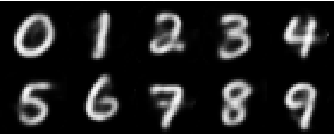
It is then particularly easy to visualize what each component represents by tweaking the components of $C$ around $0.5$; there is no need to distort real images as in [22]. Also, in our case, as mentioned in Section 2.2, the range $[0.5-2m/\sqrt{n},0.5+2m/\sqrt{n}]$ is suitable to tweak the parameters, while these ranges are not predictable with CapsNet and may vary from one feature to another, as it can be inferred from [23, 32] where the capsules of a class do not necessarily fall close to each other. The range in question $[0.5-2m/\sqrt{n},0.5+2m/\sqrt{n}]$ is actually confirmed by looking at the distributions of the individual features embodied in the capsules. On MNIST, HitNet captures some features that are positional characteristics, others can be related to the width of the font or to some local peculiarities of the digits, as in [22]. Sampling random capsules close to $C$ for a given class thus generates new images whose characteristics are combinations of the characteristics of the training images. It thus makes sense to encompass all the capsules of training images of that class in a convex space, as done with HitNet, to ensure the consistency of the images produced, while CapsNet does not guarantee this behavior ([23, 32]).

Let us note that, as underlined in [17], the reconstructions obtained for Fashion-MNIST lacks details and those of CIFAR10 and SVHN are somehow blurred backgrounds; this is also the case for the prototypes. We believe that at least three factors could provide an explanation: the decoder is too shallow, the size of the capsules is too short, and the fact that the decoder has to reconstruct the whole image, including the background, which is counterproductive.

Hybrid data augmentation

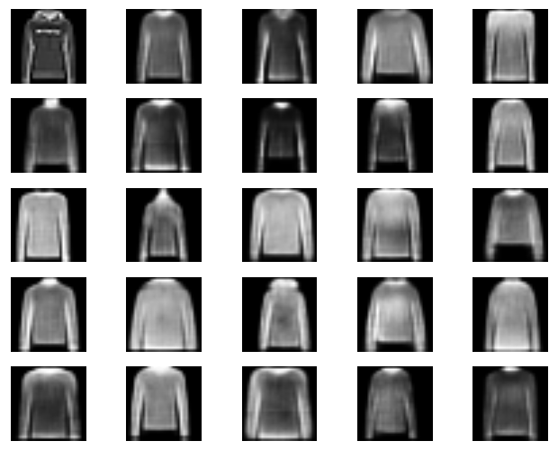
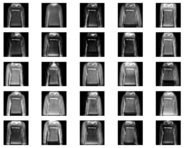
The quality of the data generated as described above depends on multiple factors, such as the number of features extracted and the quality of the decoder. Given a restricted amount of information, that is, capsules of size $16$, the decoder can only reconstruct approximations of initial images, which may not look realistic enough in some contexts. In order to incorporate the details lost in the computation of HoM, the hybrid feature-based and data-based data augmentation technique described in Section 2.2 can be applied. The importance of adding the details and thus the benefits over the sole data generation process can be visualized in Figure 5 with the FashionMNIST dataset.

(a)

(b)

(c)

(d)

Figure 5: Examples of hybrid data augmentation using the Fashion-MNIST dataset (the resolution is increased for more visual comfort). In (a) and (b), the top left image is an original image $X$ from the dataset and the image on its right is its corresponding reconstruction $X_{\text{rec}}$ from HoM (these images are the same in (a) and (b)). In (a), the $23$ remaining images are modified versions of $X_{\text{rec}}$ obtained by tweaking the components of its capsule in HoM. These images correspond to $23$ examples of $X_{\text{mod}}$. We can see that they do not contain any detail but rather serve as a skeleton on which the details $X-X_{\text{rec}}$ should be added. Adding these details to each of them gives the $23$ remaining images of (b), thus displaying $X_{\text{mod}}+X-X_{\text{rec}}$, clipped to the $[0,1]$ range, which are the images generated by the hybrid data augmentation explained in the text. The same process is shown with a different original image $X$ in (c) and (d). We can see that adding the details allows to generate convincing detailed images.

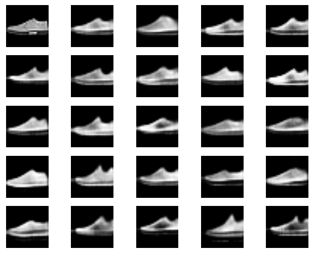
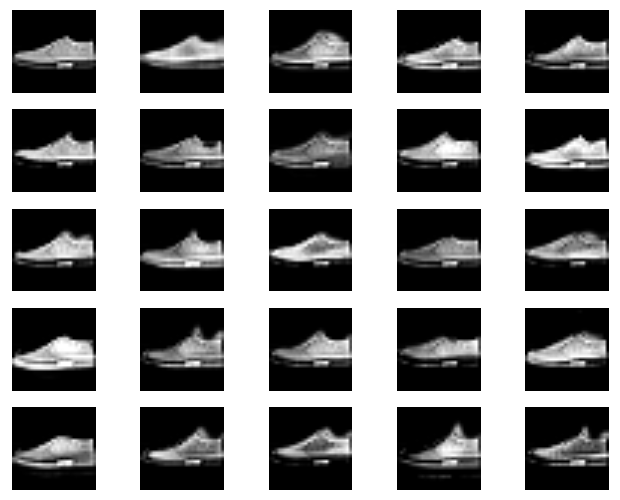
The classification performances can be marginally increased with this data augmentation process as it appeared that networks trained from scratch on such data (continuously generated on-the-fly) perform slightly better than when trained with the original data. On MNIST, the average error rate on $20$ models decreased to $0.33\%$ with a constant learning rate and to $0.30\%$ with a decreasing learning rate. In our experiments, $3$ of these models converged to $0.26\%$, one converged to $0.24\%$. Some runs reached $0.20\%$ test error rate at some epochs. With a bit of luck, a blind selection of one trained network could thus lead to a new state of the art, even though it is known that MNIST digits classification results will probably not reach better performances due to inconsistencies in the test set. The average test error rate on Fashion-MNIST decreases by $0.2\%$, on CIFAR10 by $1.5\%$ and on SVHN by $0.2\%$. These results could presumably be improved with more elaborate feature maps extractors and decoders, given the increased complexity of these datasets. The data augmentation is not performed on affNIST since the purpose of this dataset is to measure the robustness of the network to (affine) transformations.

	MNIST	Fashion-MNIST	CIFAR10	SVHN
HitNet	0.38	7.70	26.70	5.50
HitNet with DA	0.33	7.50	25.20	5.30
HitNet with DA and dlr (best)	0.24	-	-	-

Table 3: Test error rates obtained with the hybrid data augmentation (DA) process, showing slightly better performances. On MNIST, we obtained state-of-the-art performance with a decreasing learning rate.

3.3 Analyzing a training set and detecting possibly mislabeled images with ghost capsules

In this section, we illustrate the use of ghost capsules described in Section 2.3 to analyze the training set of MNIST and detect potentially erroneous labels. We train HitNet $20$ times with GC, which gives us $20$ models, and we examine the $20$ GC associated with each image by these models.

Agreement between the models

We first study the agreement between the models about the $20$ GC classes selected for each image. For that purpose, we examine the distribution of the number of different classes $N_{c}$ given to the $20$ GC of each image. It appears that the $20$ models all agree ($N_{c}=1$) on the same GC class for $28\%$ of the training images, which represents $16.859$ images.

To refine our analysis, we now focus on the $16.859$ images that have all their GC in the same class ($N_{c}=1)$ and that potentially make some hits. These images have a pair (true class, GC class) and their distribution suggests that some pairs are more likely to occur, such as $(3,5)$ for $2333$ images, $(4,9)$ for $2580$ images, $(7,2)$ for $1360$ images, $(9,4)$ for $2380$ images, which gives a glimpse of the classes that might be likely to be mixed up by the models. Confusions may occur because of errors in the true labels, but since these numbers are obtained on the basis of an agreement of $20$ models trained from the same network structure, this may also indicate the limitations of the network structure itself in its ability to identify the different classes. However, a deeper analysis is needed to determine if these numbers indicate a real confusion or not, that is, which of them make hits and which do not.

So far, we know that for these $16.859$ images, the $20$ models agree on one GC class ($N_{c}=1)$. We can examine if the $20$ models agree on their distance from $C$ for their class. For that purpose, for each image, we compute the mean and the standard deviation of its $20$ GC distances from $C$. An interesting observation is that when the mean distance gets closer to the hit zone threshold (which is $m=0.1$), then the standard deviation decreases, which indicates that all the models tend to agree on the fact that a hit is needed. This is particularly interesting in the case of mislabeled images (examples are provided hereafter, in Figure 6). Indeed, if an image of a “4” is labeled as “5” (confusion), not only are the $20$ models likely to provide $20$ GC with the same class (“4” here), but they will also all make a hit in that class “4” and thus identify it as a highly doubtful image.

Identification of doubtful images

We can now narrow down the analysis to the images that are the most likely to be mislabeled, that is, those with a mean distance smaller than $m$; there are only $71$ such images left. The associated pairs (true class, GC class) are given in Table 4. From the expected confusions mentioned above $(3,5)$, $(4,9)$, $(7,2)$, $(9,4)$, we can see that $(7,2)$ is actually not so much represented in the present case, while the pairs $(1,7)$ and $(7,1)$ subsisted in a larger proportion, and that the pairs $(4,9)$ and $(9,4)$ account for almost half of the images of interest.

		True class										Total
		0	1	2	3	4	5	6	7	8	9
GC class	0	0	0	0	0	0	0	0	0	0	0	0
	1	0	0	0	0	2	0	0	6	0	0	8
	2	0	0	0	0	0	0	0	1	0	0	1
	3	0	0	0	0	0	2	0	0	0	0	2
	4	0	0	0	0	0	0	1	0	0	20	21
	5	0	0	0	8	0	0	1	0	0	0	9
	6	0	0	0	0	0	2	0	0	0	0	2
	7	0	7	2	0	1	0	0	0	0	2	12
	8	0	0	0	1	0	0	0	0	0	0	1
	9	0	0	0	1	13	0	0	1	0	0	15
Total		0	7	2	10	16	4	2	8	0	22	71

Table 4: Distribution of pairs (true class, GC class) for MNIST training images having a unique GC class and their mean distance from $C$ smaller than the hit zone threshold.

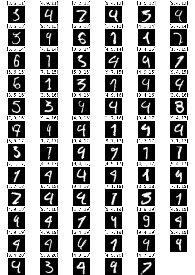
The last refinement that we make is a look at the number of hits among the $20$ GC of these $71$ images. We know that their mean distance from $C$ is smaller than $m$, but neither this mean distance nor the standard deviation clearly indicate how many of the $20$ models actually make a hit for these $71$ images. It appears that all these images have at least $55\%$ $(11/20)$ of their GC in the hit zone and that more than $75\%$ $(55/71)$ of the images have a hit for at least $75\%$ $(15/20)$ of the models, which indicates that when the mean distance is smaller than $m$, it is the result of a strong agreement between the models. Finally, the $71$ images, sorted by number of hits, are represented in Figure 6. The true label, the GC class, and the number of hits are indicated for each image. Some of these images are clearly mislabeled and some are terribly confusing by looking almost the same but having different labels, which explains the GC class selected and the number of hits obtained. While pursuing a different purpose, the DropMax technique used in [13] allowed the authors to identify “hard cases” of the training set which are among the $71$ images represented in Figure 6.

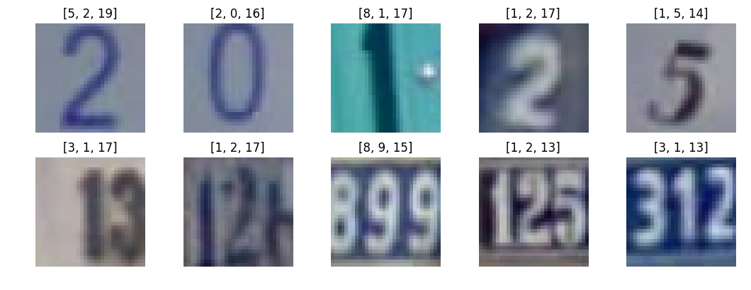
Following the same process as above, we use ghost capsules with SVHN. Again, we are able to detect images that are clearly mislabeled, as seen in Figure 6. In addition, in this case, the use of ghost capsules allows us to detect images that deserve multiple labels since multiple digits are present in the images, as seen in Figure 6.

(a)

(b)

Figure 6: (a) The $71$ images (resolution is increased for more visual comfort) of MNIST training set whose $20$ GC have a mean distance from $C$ smaller than the hit zone threshold, sorted by an increasing number of hits. The three numbers in brackets indicate respectively the true label, the GC class, the number of hits in the GC class. (b) A selection of images of SVHN obtained following the same process with ghost capsules. In the first row, the images are clearly mislabeled. In the second row, the images deserve several labels.

Ghost capsules could be used in other contexts. For example, we could imagine that a human annotator hesitates between two classes in the labelling process because the image is confusing. The annotator chooses one class and the ghost capsule deals with the confusion by potentially choosing the other class without penalizing the network. In another scenario, several annotators may give two different labels for the same image. We could handle this potential conflict with ghost capsules, by first attributing the image one of the labels suggested by the annotators (e.g. the most suggested) then training the network and finally checking whether the ghost capsule of that image is associated with the other label suggested and, if so, whether it makes a hit or not.

4 Conclusion

We introduce HitNet, a deep learning network characterized by the use of a Hit-or-Miss layer composed of capsules, which are compared to central capsules through a new centripetal loss. The idea is that the capsule corresponding to the true class has to make a hit in its target space, and the other capsules have to make misses. The novelties reside in the reinterpretation and in the use of the HoM layer, which provides new insights on how to use capsules in neural networks. Besides, we present two additional possibilities of using HitNet. In the first one, we explain how to build prototypes, which are class representatives, how to deform them to perform data generation, and how to set up a hybrid data augmentation process. This is done by combining information from the data space and from the feature space. In the second one, we design ghost capsules that are used to allow the network to alleviate the loss of capsules related to plausible alternative classes.

In our experiments, we demonstrate that HitNet is capable of reaching state-of-the-art performances on MNIST digits classification task with a shallow architecture and that HitNet outperforms the results reproduced with CapsNet on several datasets, while being at least $10$ times faster. The convergence of HitNet does not need to be forced by a decreasing learning rate mechanism to reach good performances. HitNet does not seem to suffer from overfitting, and provides a small variability in the results obtained from several runs. We also show how prototypes can be built as class representatives and we illustrate the hybrid data augmentation process to generate new realistic data. This process can also be used to marginally increase classification performances. Finally, we examplify how the ghost capsules help identifying suspicious labels in the training set, which allows to pinpoint images that should be considered carefully in the training process.

Future work

As far as the classification performances are concerned, one of the main advantages of the HoM layer is that is can be incorporated in any other network. This implies that the sub-part of HitNet used to compute the feature maps that are fully connected to HoM can be replaced by more elaborate networks to increase the performances on more complex tasks.

In a similar way, the prototypes and all the reconstructions made by the decoder could be improved by using a more advanced decoder sub-network and capsules with more components. In real-life cases such as CIFAR10 and SVHN, it could also be useful to make a distinction between the object of interest and the background. For example, features designed to reconstuct the background only could be used. If segmentation masks are available, one could also use the capsules to reconstruct the object of interest in the segmented image, or simply the segmentation mask. One could also imagine to attach different weights to the features captured by the capsules, so that those not useful for the classification are used in the reconstruction only. The flexibility of HoM allows to implement such ideas easily.

Regarding ghost capsules, they could be used to perform a built-in top-k classification, by using $k$ ghost capsules in the training process. In a binary classification task, they could be used only after a given number of epochs, which would make more sense than using them at the beginning of the training. The ghost capsule could also generate some loss but with a given probability to take into account the fact that it does not correspond to the true class and that is should be penalized in some way.

Comparing the results on other benchmark datasets would help promoting HitNet in a near future as well.

Acknowledgements

We are grateful to M. Braham for introducing us to the work of Sabour et al. and for all the fruitful discussions.

This research is supported by the DeepSport project of the Walloon region, Belgium. A. Cioppa has a grant funded by the FRIA, Belgium. We also thank NVIDIA for the support.

References

- [1] P. Afshar, A. Mohammadi, and K. Plataniotis. Brain tumor type classification via capsule networks. CoRR, abs/1802.10200, February 2018.
- [2] P.-A. Andersen. Deep reinforcement learning using capsules in advanced game environments. CoRR, abs/1801.09597, January 2018.
- [3] M. Bahadori. Spectral capsule networks. In International Conference on Learning Representations (ICLR), April-May 2018. Withdrawn paper.
- [4] J. Deng, W. Dong, R. Socher, L. Li, K. Li, and L. Fei-Fe. ImageNet: A large-scale hierarchical image database. In IEEE International Conference on Computer Vision and Pattern Recognition (CVPR), pages 248–255, Miami, Florida, USA, June 2009.
- [5] X. Guo. CapsNet-Keras. https://github.com/XifengGuo/CapsNet-Keras, 2017.
- [6] G. Hinton, A. Krizhevsky, and S. Wang. Transforming auto-encoders. In International Conference on Artificial Neural Networks (ICANN), volume 6791 of Lecture Notes in Computer Science, pages 44–51. Springer, 2011.
- [7] G. Hinton, S. Sabour, and N. Frosst. Matrix capsules with EM routing. In International Conference on Learning Representations (ICLR), Vancouver, BC, Canada, April-May 2018.
- [8] S. Ioffe and C. Szegedy. Batch normalization: Accelerating deep network training by reducing internal covariate shift. In International Conference on Machine Learning (ICML), pages 448–456, Lille, France, July 2015.
- [9] A. Krizhevsky. Learning multiple layers of features from tiny images, 2009. Technical report, University of Toronto.
- [10] R. Lalonde and U. Bagci. Capsules for objects segmentation. CoRR, abs/1804.04241, May 2018.
- [11] Y. Lecun, L. Bottou, Y. Bengio, and P. Haffner. Gradient-based learning applied to document recognition. Proceedings of IEEE, 86(11):2278–2324, November 1998.
- [12] Y. LeCun, Fu Jie Huang, and L. Bottou. Learning methods for generic object recognition with invariance to pose and lighting. In IEEE International Conference on Computer Vision and Pattern Recognition (CVPR), volume 2, pages 97–104, Washington, DC, USA, June-July 2004.
- [13] H. Lee, J. Lee, S. Kim, E. Yang, and S. Hwang. DropMax: Adaptive variational softmax. CoRR, abs/1712.07834, December 2017.
- [14] Y. Li, M. Qian, P. Liu, Q. Cai, X. Li, J. Guo, H. Yan, F. Yu, K. Yuan, J. Yu, L. Qin, H. Liu, W. Wu, P. Xiao, and Z. Zhou. The recognition of rice images by UAV based on capsule network. Cluster Computing, pages 1–10, March 2018.
- [15] H. Liao. CapsNet-Tensorflow. https://github.com/naturomics/CapsNet-Tensorflow, 2018.
- [16] W. Liu, E. Barsoum, and J. Owens. Object localization and motion transfer learning with capsules. CoRR, abs/1805.07706, May 2018.
- [17] P. Nair, R. Doshi, and S. Keselj. Pushing the limits of capsule networks. Technical note, 2018.
- [18] Y. Netzer, T. Wang, A. Coates, A. Bissacco, B. Wu, and A. Ng. Reading digits in natural images with unsupervised feature learning. In Advances in Neural Information Processing Systems (NIPS), volume 2011, Granada, Spain, December 2011.
- [19] J. O’Neill. Siamese capsule networks. CoRR, abs/1805.07242, May 2018.
- [20] L. Perez and J. Wang. The effectiveness of data augmentation in image classification using deep learning. CoRR, abs/1712.04621, December 2017.
- [21] D. Rawlinson, A. Ahmed, and G. Kowadlo. Sparse unsupervised capsules generalize better. CoRR, abs/1804.06094, April 2018.
- [22] S. Sabour, N. Frosst, and G. Hinton. Dynamic routing between capsules. CoRR, abs/1710.09829, October 2017.
- [23] A. Shahroudnejad, A. Mohammadi, and K. Plataniotis. Improved explainability of capsule networks: Relevance path by agreement. CoRR, abs/1802.10204, February 2018.
- [24] T. Shin. CapsNet-TensorFlow. https://github.com/shinseung428/CapsNetTensorflow, 2018.
- [25] N. Srivastava, G. Hinton, A. Krizhevsky, I. Sutskever, and R. Salakhutdinov. Dropout: A simple way to prevent neural networks from overfitting. Journal of Machine Learning Research, 15(1):1929–1958, January 2014.
- [26] T. Tieleman. affNIST. https://www.cs.toronto.edu/ tijmen/affNIST/, 2013.
- [27] L. Wan, M. Zeiler, S. Zhang, Y. Le Cun, and R. Fergus. Regularization of neural networks using dropconnect. In International Conference on Machine Learning (ICML), volume 28, pages 1058–1066, Atlanta, Georgia, USA, June 2013.
- [28] D. Wang and Q. Liu. An optimization view on dynamic routing between capsules. In International Conference on Learning Representations (ICLR), Vancouver, BC, Canada, April-May 2018.
- [29] Q. Wang, T. Ruan, Y. Zhou, C. Xu, D. Gao, and P. He. An attention-based Bi-GRU-CapsNet model for hypernymy detection between compound entities. CoRR, abs/1805.04827, May 2018.
- [30] S. Wong, A. Gatt, V. Stamatescu, and M. McDonnell. Understanding data augmentation for classification: When to warp? In Digital Image Computing: Techniques and Applications, pages 1–6, Gold Coast, Queensland, Australia, November-December 2016.
- [31] E. Xi, S. Bing, and Y. Jin. Capsule network performance on complex data. CoRR, abs/1712.03480, December 2017.
- [32] L. Zhang, M. Edraki, and G.-J. Qi. CapProNet: Deep feature learning via orthogonal projections onto capsule subspaces. CoRR, abs/1805.07621, May 2018.