Prediction on detection and characterization of Galactic disk microlensing events by LSST

Abstract

Upcoming LSST survey gives an unprecedented opportunity for studying populations of intrinsically faint objects using microlensing technique. Large field of view and aperture allow effective time-series observations of many stars in Galactic disk and bulge. Here, we combine Galactic models (for $|b|<10^{\rm{\circ}}$) and simulations of LSST observations to study how different observing strategies affect the number and properties of microlensing events detected by LSST. We predict that LSST will mostly observe long duration microlensing events due to the source stars with the averaged magnitude around $22$ in $r-$band, rather than high-magnification events due to fainter source stars. In Galactic bulge fields, LSST should detect on the order of $400$ microlensing events per square degree as compared to $15$ in disk fields. Improving the cadence increases the number of detectable microlensing events, e.g., improving the cadence from $6$ to $2$ days approximately doubles the number of microlensing events throughout the Galaxy. According to the current LSST strategy, it will observe some fields $900$ times during a $10-$year survey with the average cadence of $\sim 4\rm{-days}$ (I) and other fields (mostly toward the Galactic disk) around $180$ times during a $1-$year survey only with the average $\sim 1\rm{-day}$ cadence (II). We anticipate that the number of events corresponding to these strategies are $7900$ and $34000$, respectively. Toward similar lines of sight, LSST with the first observing strategy (I) will detect more and on average longer microlensing events than those observable with the second strategy. If LSST spends enough time observing near Galactic plane, then the large number of microlensing events will allow studying Galactic distribution of planets and finding isolated black holes among wealth of other science cases.

1. Introduction

The Large Synoptic Survey Telescope (LSST) is an optical and wide-field telescope whose primary mirror has $8.4\leavevmode\nobreak\ \rm{m}$ diameter and is now under construction in Chile (Ivezic et al., 2009). LSST is supposed to observe the most of the visible sky every $4$ days. Its field of view (FoV) and lifetime will be $9.6\leavevmode\nobreak\ \rm{deg^{2}}$ and $10$ years, respectively. The exposure time for each field will be $30\leavevmode\nobreak\ \rm{sec}$. During a night, LSST will observe each field twice with visits separated by $15-60$ minutes (LSST Science Collaboration et al., 2017). Hence, LSST will take about $1000$ images for most fields in the visible sky during its lifetime, i.e., the total number of visits in $10$ years is anticipated to be about $2.8$ million. Also $90$ percent of its time will be allocated to uniform observations with a constant cadence and during the rest of time, LSST will observe with other strategies.

LSST will (i) measure weak gravitational lensing to probe for any signals of dark energy and dark matter, (ii) map our galaxy and its objects, (iii) make an inventory of solar system components, and (iv) detect transient phenomena in optical band such as supernovae (Ivezic et al., 2009). However, other astrophysical events will be detected during the LSST lifetime. For instance, if Galactic disk is observed uniformly, then many microlensing events toward the Galactic bulge and disk will be detected. In this regard, Gould (2013) studied the possibility of probing the planet distribution in the Galactic plane by microlensing detection in addition to the transit technique.

When the light of a background source star passes through the gravitational field of a foreground massive object, it is bent toward the center of gravity, the so-called gravitational lensing event. In the Galactic scales, the light from a distant star can be lensed and as a result magnified by a collinear massive object which is called a gravitational microlensing event (Einstein, 1936). In these events the light from the background source star is magnified and produces two deformed images with unresolvable angular separation.

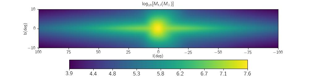
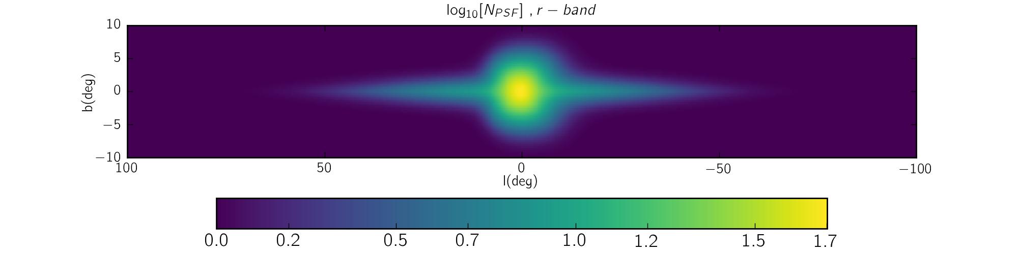
Figure 1.— Figure 1: Maps of the overall mass in the Galaxy $M_{t,l}\rm{[M_{\odot}]}$, which is the integration over the cumulative mass densities due to all stellar structures from the observer up to $20\leavevmode\nobreak\ \rm{kpc}$ toward each line of sight. Every line of sight covers the area $\Omega_{l}=(0.25\leavevmode\nobreak\ \rm{deg})^{2}$. Figure 1: the averaged number of collinear stars whose light enters the LSST PSF of a typical source star $N_{PSF}(l,b)$. The averaging is done over the detectable microlensing events.

Detecting microlensing events toward the Galactic disk by a survey telescope helps constraining the mass, spatial and velocity stellar distributions in the Galactic thin and thick disks and the Galactic bar. Probing microlensing events during $7$ seasons toward $4$ directions in the Galactic plane was done by EROS-II (Rahal et al., 2009). As a result of this project, $27$ microlensing candidates have been found. By performing a Monte Carlo simulation according to the EROS-II observing strategy and comparing the results from simulation with the real observation, Moniez et al. (2017) could test the Galactic models, different mass functions, etc. The problems with microlensing events toward the Galactic plane are: (i) we do not know source distances, whereas toward the Galactic bulge almost all of the source stars belong to the Galactic bulge and are located at the distance of approximately $8\leavevmode\nobreak\ \rm{kpc}$ far from us and (ii) the interstellar extinction is high and variable in both quantity and quality toward the Galactic disk. We lack detailed knowledge about extinction in the disk because there is no group of stars for which we apriority know colors and can be easily selected (red clump stars serve in the bulge). The poorly known extinction hampers optimizing observations and makes determination of event properties harder, (i.e., the source angular size, the size of the Einstein ring). These issues increase the number of degenerate physical parameters. However, the overall distributions of the observable parameters from observations can be used to examine the different models in the Galaxy.

LSST is suppose to uniformly observe the galactic plane. As a result, it will detect large number of microlensing events toward the Galactic disk and bulge and its results will help to probe different Galactic models of mass, velocity, special distribution, etc. In this work, we aim to simulate LSST observations toward the the Galactic bulge and disk with its observing strategies to predict detections of the Galactic disk microlensing events. We aim to specify the characteristics and statistics of the disk microlensing events which will be detected during its era. However, we do not consider the case of LSST providing supporting observations for the WFIRST microlensing survey to measure free-floating planet masses.

We perform a Monte Carlo simulation of detectable microlensing events during the LSST lifetime according to its observing strategy in details explained in section (2). In the following section, we discuss the optical depth, the rate of events and the number of observable events toward different directions resulted from the simulation. Also we discuss the impact of observing cadence on the results. In the section (4), we simulate observing microlensing events by considering two strategies for observation (I) $900$ epochs during $10$ years observation with the $3.9\rm{-day}$ cadence and (II) $180$ epochs during the first year with the $0.9\rm{-day}$ cadence, to predict statistics and properties of detectable microlensing events with these strategies. We summarize the results and conclude in the section (5).

2. Modeling of LSST microlensing observations

In order to simulate the microlensing events detectable by LSST, we (i) simulate an ensemble of model microlensing events toward different directions in the Galactic plane, (ii) generate synthetic data points for each of them by assuming that these events are being observed by LSST, and finally (iii) exert some criteria as detectability threshold to simulated microlensing events to determine (a) the LSST ability of detecting bulge and disk microlensing events and (b) the characteristics of these events. These three steps are discussed in the following subsections, respectively.

2.1. Simulating disk microlensing events

In the following, we illustrate how to generate the parameters of the source and the lens stars to make microlensing model light curves. For the source stars, their locations are specified according to the overall mass density throughout the Galaxy versus distance in a given direction $dM/dD_{s}\propto\rho_{t}(l,b,D_{s})D^{2}_{s}\Omega_{l}$, where $\rho_{t}(D_{s})$ is total mass density due to all stellar structures in our galaxy, i.e., the thin and thick disks, Galactic bulge (and bar), and the stellar halo, $D_{s}$ is the source distance from the observer, and $l$ and $b$ represent the Galactic longitude and latitude respectively. We model these mass densities using the Besançon model (Robin et al., 2003, 2012). One can find all details of these mass density profiles in the Appendix B of Moniez et al. (2017). The map of total mass $M_{t,l}=\int_{D_{s}}\rho_{t}(l,b,D_{s})D_{s}^{2}\leavevmode\nobreak\ dD_{s}\leavevmode\nobreak\ \Omega_{l}$ in the unit of $M_{\odot}$ per line of sight in the Galaxy is shown in Figure 1. In the simulation, the area corresponding to each line of sight is $\Omega_{l}=(0.25\leavevmode\nobreak\ \rm{deg})^{2}$.

We indicate the intrinsic photometric properties of the source stars in the same way as Penny et al. (2017) and use the old public version of the Besançon model. For each structure, we simulate a sample of stars in CFHTLS-Megacam photometry system without considering extinction. Then, the magnitudes in these filters, $u^{\star}g^{\prime}r^{\prime}i^{\prime}z^{\prime}$, are converted to the magnitudes in the Sloan Digital Sky Survey (SDSS) filters as (Gwyn, 2008):

$$u^{\star} = u-0.241\leavevmode\nobreak\ (u-g),$$

$$g^{\prime} = g-0.153\leavevmode\nobreak\ (g-r),$$

$$r^{\prime} = r-0.024\leavevmode\nobreak\ (g-r),$$

$$i^{\prime} = i-0.085\leavevmode\nobreak\ (r-i),$$

$$z^{\prime} = z+0.074\leavevmode\nobreak\ (i-z);$$ (1)

LSST filters are the same as the SDSS photometry system (Ivezic et al., 2009; Fukugita et al., 1996). These magnitudes can also be transformed to the standard Johnson-Cousins photometry system. We do not simulate the magnitude of source stars in the $y-$band filter. The Besançon model does not give the magnitude of stars in this band. However, the LSST photometric uncertainty in this band is high, i.e., the 5$\sigma$ depth for point sources in $y-$band, $m_{5,y}$, is $22.6$ whereas that for $z-$band is $24.45$.

In order to determine the apparent magnitude of the source stars, we add the distance modulus and the extinction due to the interstellar gas and dust to the absolute magnitudes. We use the 3D extinction map presented by Marshal et al. (2006). They measured 3D $K_{s}-$extinction map for the Galactic latitude in the range of $b\in[-10:10^{\rm{\circ}}]$ and the Galactic longitude in the range of $l\in[-100:100^{\rm{\circ}}]$ with the step $\Delta b=\Delta l=0.25^{\mathrm{\circ}}$ and the distance step $0.5\leavevmode\nobreak\ \rm{kpc}$. Then, we convert it to the extinction in $K-$band using $A_{K}=0.95\leavevmode\nobreak\ A_{K_{s}}$ (Marshall et al., 2006). The $K-$band extinction is converted to the extinction in other bands using Cardelli et al.(1989)’s relations. We assume $R_{V}$ of $2.5$ for Galactic bulge and $3.1$ for thin disk, thick disk, and the stellar halo (Nataf et al., 2013; Cardelli et al., 1989). We also add a Gaussian fluctuation to each extinction value with the width in the range $[0.017,0.04]$ depending on the wavelength (Cardelli et al., 1989). The source radius $R_{\star}$ is estimated using the Stefan-Boltezman relation: $L=\sigma T^{4}_{eff}4\pi R^{2}_{\star}$, where $L$ is the source luminosity, $T_{eff}$ is the effective surface temperature and $\sigma$ is the Stefan-Boltzmann constant.

The blending effect in the LSST observations is significant, because this telescope is anticipated to detect stars as faint as those with $24.3\leavevmode\nobreak\ \rm{mag}$ in $r-$band. The number of such faint stars in the Galaxy is very high, which makes high blending effects for these faint stars. Therefore, it is crucial to consider and accurately calculate the blending amount for each source star. In order to calculate the contribution of background stars in the each LSST Point Spread Function (PSF), we calculate the averaged number of collinear stars toward the source line of sight whose light enters the PSF area which is given by:

$$N_{PSF}(l,b)=\int_{D_{s}}\leavevmode\nobreak\ n_{t}(l,b,D_{s})\leavevmode\nobreak\ dD_{s}\leavevmode\nobreak\ D_{s}^{2}\leavevmode\nobreak\ \Omega_{PSF},$$ (2)

where $\Omega_{PSF}=\pi(\mathrm{FWHM}/2)^{2}$ in square arcsec is the LSST PSF area for a typical source star. $\mathrm{FWHM}$ is the Full Width at the Half Maximum of the brightness profile due to a typical source star which is $(1.22,1.10,0.99,0.97,0.95)$ in arcsec unit corresponding to the filters $ugriz$, respectively. The $n_{t}(l,b,D_{s})$ is the total number density of stars in a given direction and at the distance $D_{s}$ from the observer, which is given by:

$$n_{t}(l,b,D_{s})=\sum_{i=1}^{4}\leavevmode\nobreak\ \frac{\rho_{i}(l,b,D_{s})}{<M_{i}>}$$ (3)

where $\rho_{i}(l,b,D_{s})$ is the mass density for the $i$th structure of our galaxy, $<M_{i}>$ is the averaged mass amount for the $i$th structure and the summation is done over different structures. The equation (2) gives the average number of blending stars and the true number in each measurement has a gaussian fluctuation around this value with the width $\sqrt{N_{\rm{PSF}}}$. Figure 1 represents the map of $N_{\rm{PSF}}(l,b)$ in the Galaxy averaged over $N_{\rm{PSF}}$ of observable microlensing events. For each of these blending stars, we calculate their apparent magnitudes as explained in the previous paragraph and as a result the overall flux due to all of blending stars, i.e., $F_{base}=\sum_{i=1}^{N_{PSF}}10^{-0.4\leavevmode\nobreak\ m_{i}}$. One of these blending stars is the source star itself. The blending parameter is given by $f_{b}=F_{\star}/F_{base}$, where $F_{\star}=10^{-0.4m_{\star}}$ is the flux of the source star. In the real observation, if the overall magnitude due to all blending stars into a PSF reaches to the detection threshold, in that PSF one star is discerned, whereas in the simulation all of these blending stars pass the detectability criterion. In order to accordingly correct the simulation, we weight each simulated source star with its blending factor $f_{b}$.

For the lens population, we first indicate the lens distance from the observer $D_{l}$ using the lensing probability function $d\Gamma/dD_{l}\propto\rho_{t}(D_{l})\sqrt{D_{l}(D_{s}-D_{l})/D_{s}}$. According to the contribution of different structures in the total mass density at the location of the lens $\rho_{t}(D_{l})$, we determine to which structure the lens belongs to. Then, the lens mass is chosen from the corresponding mass density function to the lens structure. The Besançon model provides separate mass functions for different structures. We assume both source and lens stars have global and dispersion velocities (Kayser et al., 1986; Binney & Tremaine, 2008). In order to determine the lens-source relative velocity, we (i) obtain the velocity components in the observer coordinate system which axes are parallel with and normal to the line of sight direction and (ii) after projecting the source velocity in the lens plane subtract each component of the lens and source velocities. In the Besançon model, the values of different components of dispersion velocities depend on the stellar age and structure. In the simulation, we discard the events with the Einstein crossing time shorter than $0.5$ or longer than $300$ days. The longer microlensing events are hard distinguish in real observations (see, e.g., Mróz et al., 2017; Wyrzykowski et al., 2015). The lens impact parameter is chosen uniformly from the range $[0:1]$.

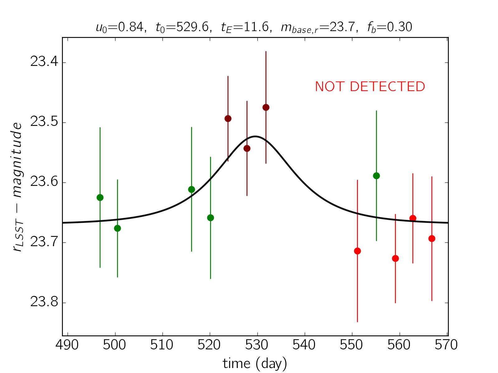
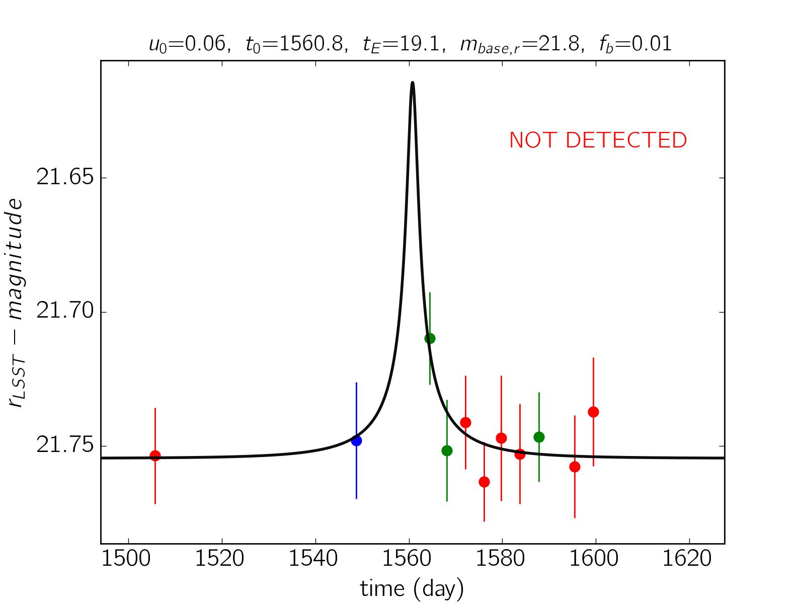
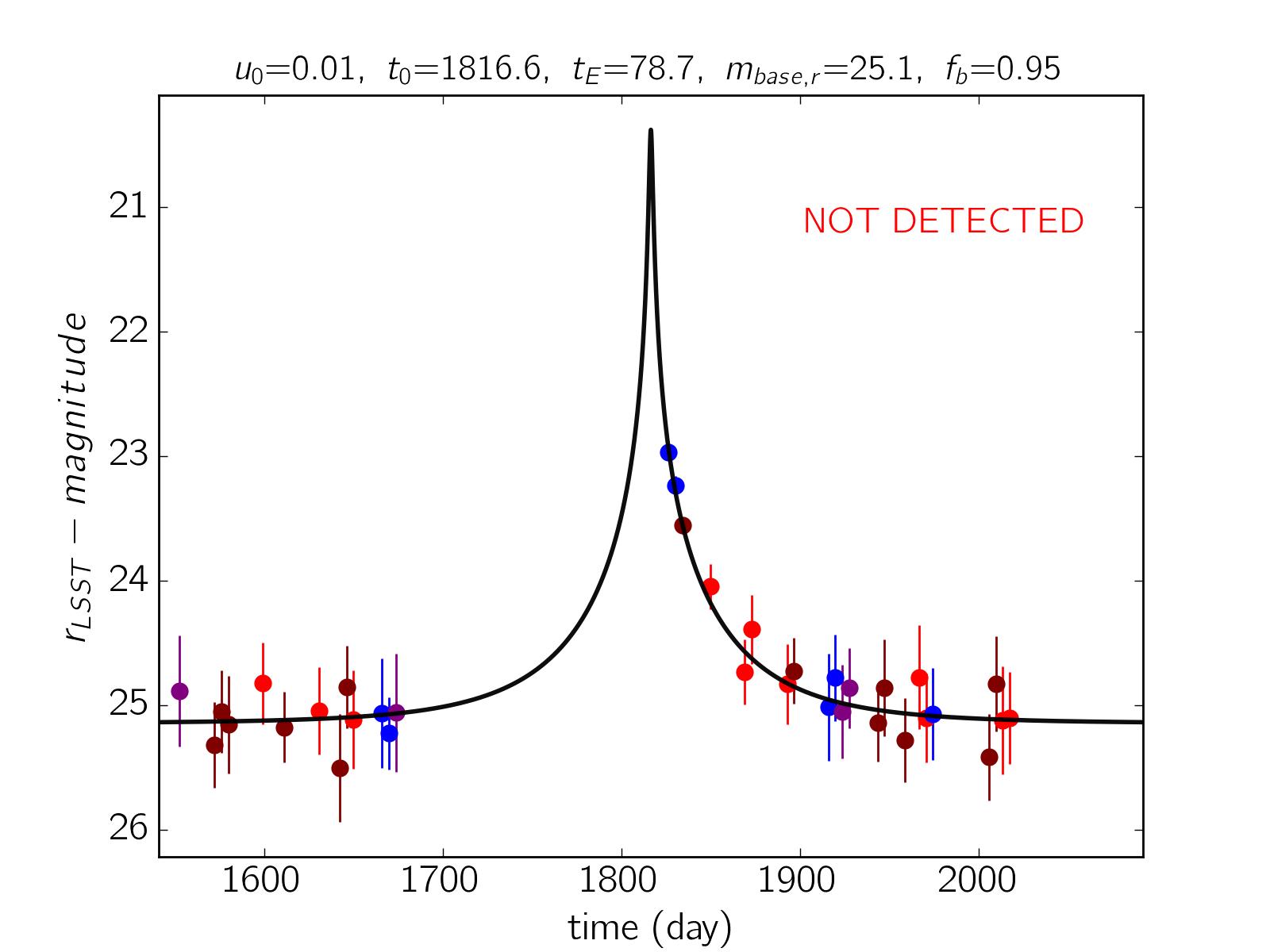
Figure 2.— Example simulated microlensing events with the synthetic data points taken by LSST which are not distinguishable. The parameters used to make each of them are mentioned at the top of each light curve. The color of data points indicates the filter used: purple, blue, green, red and brown data points are taken $ugriz$ filters respectively. The amounts of the background and intrinsic source flux depends on the filter used. We assume that these fluxes for each source star in all filters are measurable during the LSST observation. As a result, we can convert the measured magnitude in each filter to the corresponding magnitude in $r-$band and easily model all data points with one light curve.

2.2. Generating synthetic data points

After generating the model microlensing events, the observability of their source stars by LSST is checked. From simulated model microlensing events, we ignore the microlensing events (i) which source stars are too faint to be detected at least in one of the LSST filters even when they are at the peak of their light curves and (ii) which source stars are fainter than the saturation limit of LSST in all filters. These events certainly are not observable. We had the detection threshold (i.e., limiting magnitude) for different LSST filters as given by Ivezic et al. (2009) (Table 2).

In order to test the observability of microlensing signatures of the remaining microlensing events, we generate the hypothetically data points taken by LSST and then verify if they can be discerned as microlensing events by exerting some criteria. The data points are simulated in the range $[t_{0}-3.5t_{\rm{E}}:t_{0}+3.5t_{\rm{E}}]$, where $t_{\rm{E}}$ is the Einstein crossing time, $t_{0}$ is the time of the closest approach that was uniformly chosen in the range of $[0:T_{obs}]$, where $T_{obs}=10\leavevmode\nobreak\ \rm{yrs}$ is the LSST lifetime. If the start time $t_{min}$ is less than zero (i.e., $t_{min}=t_{0}-3.5t_{\rm{E}}<0$) we start simulating data points from $t_{min}=0.0$ and if the end time $t_{max}=t_{0}+3.5t_{\rm{E}}$ is greater than $T_{obs}$ we interrupt simulating data points on $T_{obs}$. The exposure time is fixed on $30\leavevmode\nobreak\ \mathrm{seconds}$. For timing the data points we also consider the seasonal gaps, i.e., the LSST observations happen only during about seven continuous months of each year. We assume that the weather is not suitable for the LSST observation with the probability of $20\%$ for each night. However, during each night, the uniform observation by LSST will take place with the probability of $90\%$ which is considered in the simulation.

For calculating the magnification factor, we consider the finite size effect of the source star and use the adaptive contouring algorithm (Dominik, 2007) to calculate the magnification while the lens distance from the source center is in the order of the source radius projected on the lens plane. The synthetic data points which are between saturation and detection limits of the LSST are considered. We ignore the microlensing parallax effect during magnification calculations.

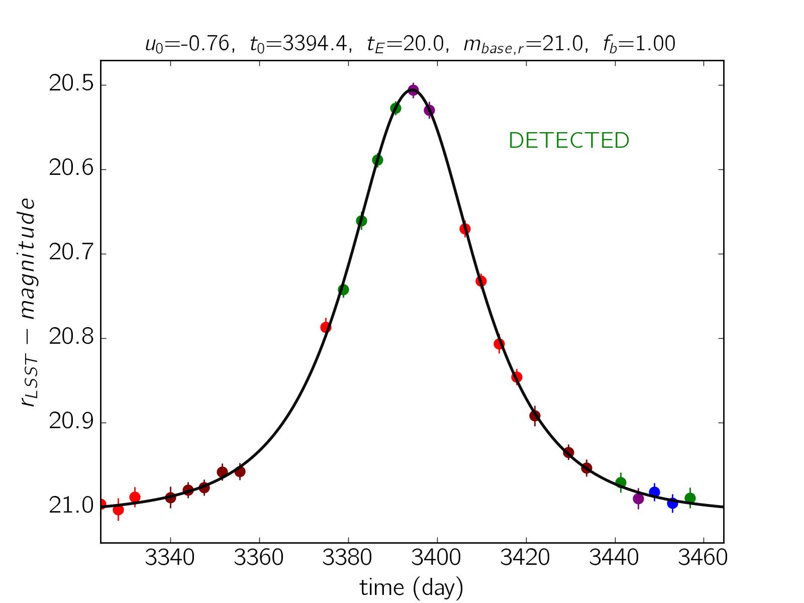
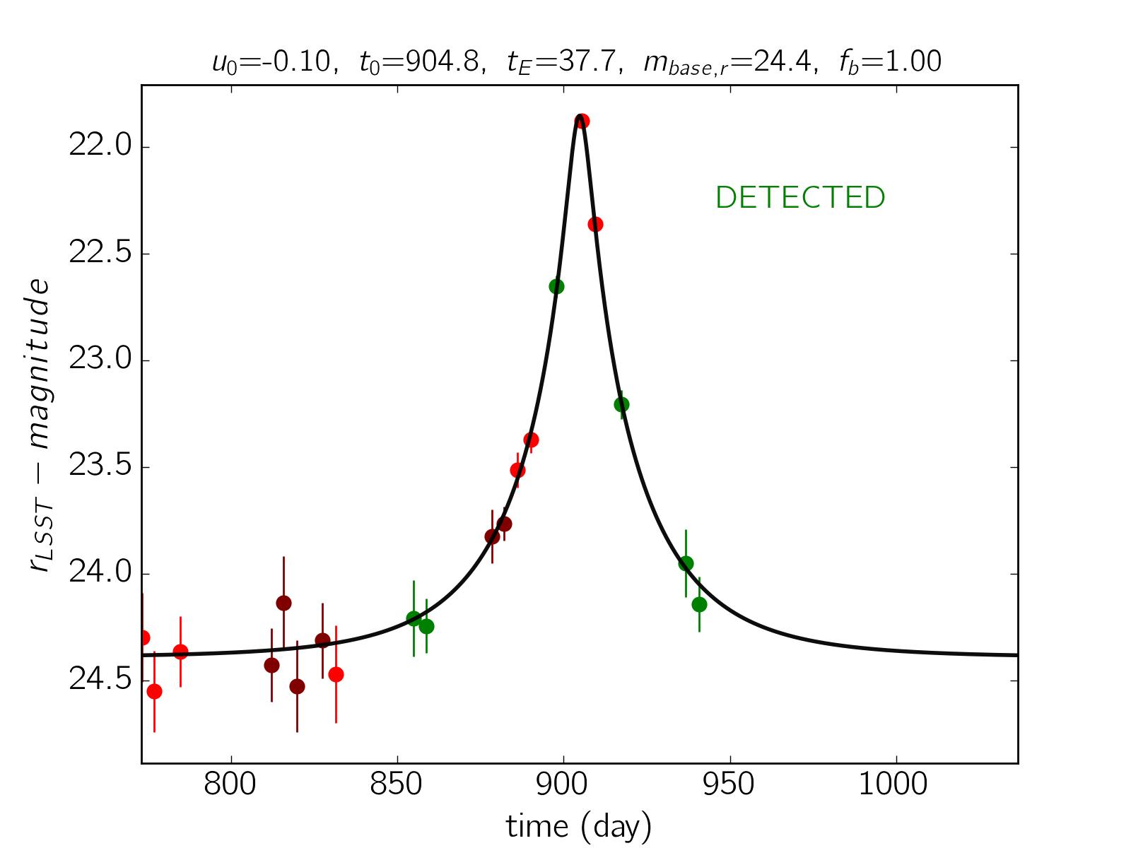
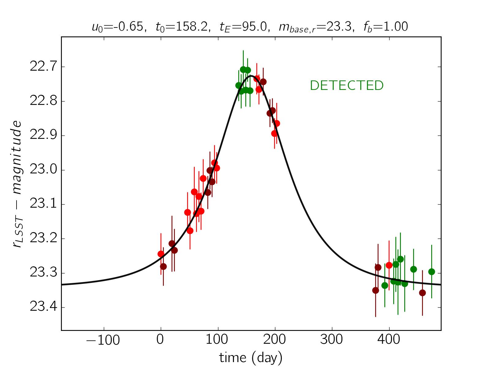
Figure 3.— Example simulated microlensing events which are detectable with LSST with the synthetic data points. More details can be found in the caption of Figure (2).

We assume that the observed magnitude of each data point has a gaussian fluctuation with respect to model value with the width equal to expected photometric error filter $j$ ($j\in ugriz$): $\sigma_{m,j}=\sqrt{\sigma^{2}_{sys}+\sigma^{2}_{rand,j}}$. The $\sigma_{m,j}$ contains the random and systematic photometric errors. We take into account these two uncertainties from Ivezic et al. (2009). For $\sigma_{rand}$ calculation we assumed sky brightness as given by Table 2 of the mentioned paper, i.e., ignoring impact of other stars and actual zenith distance. The photometric errors depend on wavelength and significantly decrease for the bright stars. In order to determine the epoch, airmass and filter used for taking each data point, we make a big ensemble of these parameters from Operations Simulator (OpSim) with the approved reference run minion${}_{-}1016$. Each data point is reported in one filter.

2.3. Detectability criteria

After generating synthetic data points of each model microlensing event, we probe if that event can be discerned. Our criteria for detectability are (i) there are at least $4$ consecutive data points (in any filter) with the observed magnification deviating from constant flux more than $5\leavevmode\nobreak\ \sigma_{m,j}$, (ii) the difference of $\chi^{2}$ from fitting the constant flux model and the microlensing model to the synthetic data points is larger than $200$, and finally (iii) the peak of the light curve should be between $t_{min}$ and $t_{max}$. As a result from the third criterion, we ignore the microlensing events for which the time of the closest approach is out of the LSST lifetime.

Six example simulated microlensing events with the synthetic data points are represented in Figures (2) and (3). The parameters used to make each of them are mentioned at the top of each light curve. $m_{base,r}$ is the baseline $r-$band brightness due to cumulative fluxes entered in the source PSF. The $t_{\rm{E}}$ and $t_{0}$ are expressed in the days. The amounts of the background and intrinsic source flux depend on the filter used. We assume that these fluxes for each source star in all filters are measurable during the LSST observation. As a result, we can convert the measured magnitude in each filter to the corresponding magnitude in $r-$band and easily model all data points with one light curve, as shown in the figures.

The first microlensing event shown in Figure 2 is not detectable by LSST, because of high blending. The source star is magnified enough, but the blending causes the enhancement in the stellar brightness due to the lensing effect to shrink and become on the order of the photometric noise. The microlensing event shown in Figure 2 is not recognizable although it is a high-magnification event. Indeed, its time scale is too short in comparison with the LSST cadence so that only a single data point is taken during the magnification. The next event represented in Figure 2 is not detectable also, although there is no blending effect and the event’s time scale is long enough. Because of the seasonal gap, the peak of the light curve is not covered by the LSST data points.

The microlensing events shown in Figure (3) are observable by LSST. The first event has the large impact parameter, i.e., small lensing effect. Most microlensing events with small blending effect and the bright source stars can be detected. The next one (represented in Figure 3) is detected. In contrast to the high-magnification microlensing event 2 which was not detectable, this high-magnification event is detected. The duration of this event is long enough to take several data points while the source star is magnified. The last microlensing event shown in Figure 3 is also recognizable. The long-duration microlensing events have higher chance to be detected during the LSST lifetime in comparison to the short duration events.

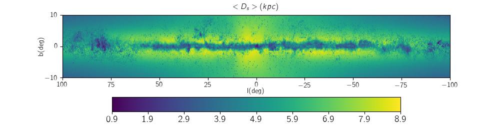
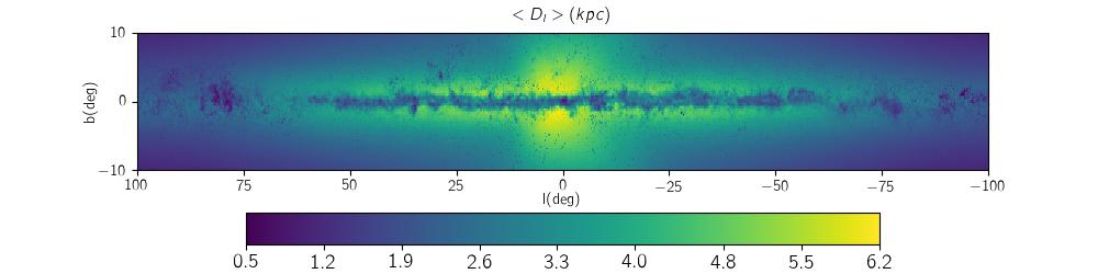
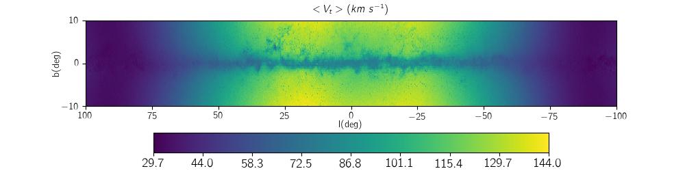
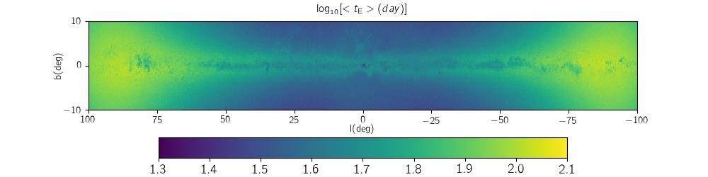
Figure 4.— Maps of physical parameters for microlensing events detectable by LSST toward the Galactic plane resulted from the Monte Carlo simulation. The parameters are the source and lens distances from the observer, the relative lens-source velocity and the Einstein crossing time from top to bottom, respectively.

Figures (2) and (3) show that the microlensing events of very faint source stars (specially those fainter than the LSST detection threshold) can not mostly be detected. These events need to be highly magnified to be detected, whereas the durations of high-magnification microlensing events are proportional to $t_{\rm{E}}u_{0}$, mostly too short in comparison with the LSST cadence. Whereas, the microlensing events of bright source stars even with low magnification or long-duration ones are more likely to be detected. For these events the time scale of the magnification is of order of the Einstein crossing time, most likely long enough for taking several data points by LSST. In the next section we study the characteristics and statistical properties of the detectable microlensing events.

3. Observable Microlensing events with LSST

For each direction specified with the Galactic longitude and latitude with the steps $\Delta(l)=\Delta(b)=0.25^{\rm{\circ}}$, we perform a Monte Carlo simulation of microlensing events and probe their detectability, so that for every direction we have an ensemble of the detected events. In the following subsection we plot the map of characterizations and statistics of these events to study them. The numbers behind these maps are listed in Table (6) and (5) of the online version.

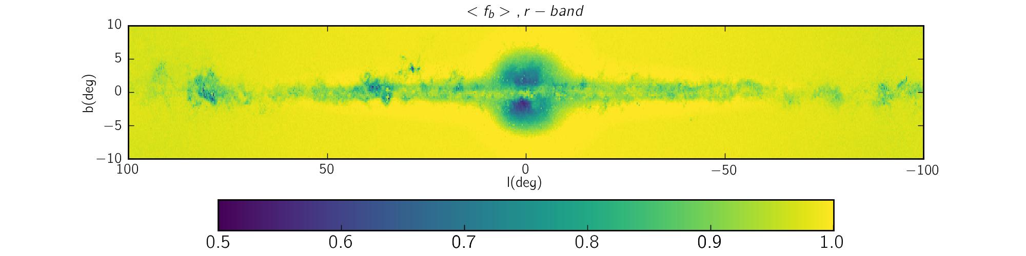
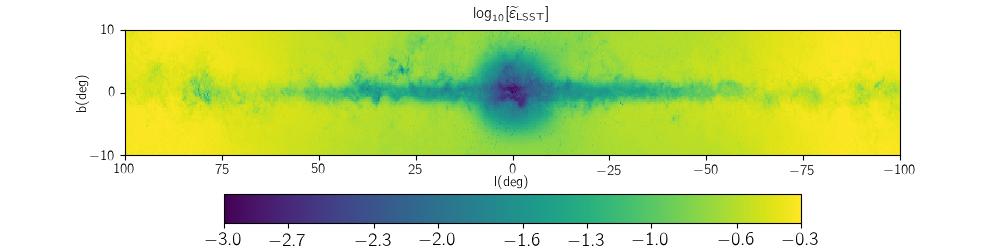
Figure 5.— Maps of the blending parameter in $r$-band of observable microlensing events (top) and the probability of detecting microlensing events $\widetilde{\varepsilon}_{\rm{LSST}}(l,b)$ (bottom), respectively.

3.1. Characterizations and statistics

In Figure (4), we plot the maps of the averaged physical parameters of the lens and source stars for the observable microlensing events. These parameters are the source and the lens distances from the observer, the relative lens-source velocity, and the Einstein crossing time from top to bottom. Toward the small latitudes ($|b|<2^{\rm{\circ}}$), the interstellar extinction is very high which causes mostly the microlensing events with closer source and lens stars to be detectable, see Figure 4 and 4. According to Figure 4, toward the Galactic bulge excluding the points with $|b|<2^{\rm{\circ}}$ most of the lens stars belong to the Galactic bulge and are located at the average distances around $6\leavevmode\nobreak\ \rm{kpc}$.

The Einstein crossing times of microlensing events far from the Galactic bulge are intrinsically much longer than those toward the Galactic bulge because the averaged relative lens-source velocity of the events far from the Galactic bulge is much smaller than that of the events toward the Galactic bulge, see Figures 4 and 4. For events that are far from the Galactic bulge on the sky, the relative lens-source velocity is smaller because the lens and source are close to each other and close to the Sun. Generally, the detectable microlensing events with LSST (due to long cadence) are a little longer than the detectable events with OGLE or MOA surveys toward similar lines of sight.

Figure (5) represents two maps: the top one, shows the blending parameter per line of sight averaged over the detectable microlensing events in $r$-band. The blending parameter $f_{b}$ is a function of the stellar number density and decreases while increasing the stellar number density (plotted in Figure 1). In the bottom map, we plot the probability of discerning microlensing events which their source stars are visible at least at one filter toward a given direction, $\widetilde{\varepsilon}_{\rm{LSST}}(l,b)$. For each line of sight, this probability is the fraction of the simulated microlensing events with detectable source stars (at least at one filter) which pass the detectability criteria (mentioned in the subsection 2.3). Generally, LSST detects the microlensing events with longer durations than typical values. Far from the Galactic bulge, the averaged Einstein timescale of microlensing events is longer than that of the events toward the Galactic bulge. On the other hand, the blending effect is ignorable toward the Galactic disk. These two effects make the probability function $\widetilde{\varepsilon}_{\rm{LSST}}(l,b)$ toward the Galactic plane be more than that toward the Galactic bulge.

For the statistics properties, we first calculate the overall optical depth due to all structures for the simulated microlensing events which are recognizable with LSST. The optical depth in given direction and distance can be calculated as (e.g., Moniez et al. (2017)):

$$\tau_{\rm{DIA}}(l,b,D_{s})=\frac{4\pi\leavevmode\nobreak\ G\leavevmode\nobreak\ D^{2}_{s}}{c^{2}}\int^{1}_{0}\leavevmode\nobreak\ x(1-x)\leavevmode\nobreak\ \rho_{t}(l,b,x)\leavevmode\nobreak\ dx,$$ (4)

where $x=D_{l}/D_{s}$. Toward the Galactic disk, the distance of the detectable sources has a wide distribution. In that case the optical depth results from averaging over optical depths due to different source distances (Rahal et al., 2009). We consider the source stars are visible at peak (but not at baseline), the so-called DIA optical depth (Kerins et al., 2009), $\tau_{\rm{DIA}}(l,b)$. The maps of the DIA optical depth is shown in Figures 6. The DIA optical depth is reduced in $|b|<2^{\circ}$ region due to the high extinction and blending, which prevent detection of events with sources at large distances.

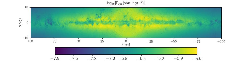
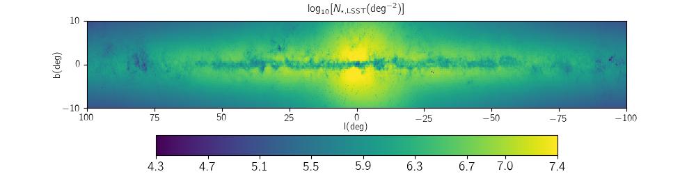
Figure 6.— Statistics of microlensing parameters for LSST Galactic plane events. These statistical parameters are the DIA optical depth, the observing rate of events detectable by the LSST per year, per star, the number of background stars detectable in at least one of the LSST filters per square degree and the number of detected microlensing events per year per square degree from top to bottom, respectively. In the last panel, the values of $\log_{10}[N_{e}]$ smaller than $-2$ are marked same as $-2$ and the smallest recorded value is $-3.5$.

Using the DIA optical depths, we estimate the observed event rate per line of sight as:

$$\Gamma_{\rm{obs}}(l,b)=\frac{2}{\pi}\left<\frac{\varepsilon_{\rm{LSST}}(l,b,t_{\rm{E}})}{t_{\rm{E}}}\right>\leavevmode\nobreak\ \tau_{\rm{DIA}}(l,b),$$ (5)

where $\varepsilon_{\rm{LSST}}(l,b,t_{\rm{E}})$ is the LSST efficiency for detecting microlensing events with the duration $t_{\rm{E}}$ toward a given direction. Indeed, this function is the mentioned probability function $\widetilde{\varepsilon}_{\rm{LSST}}(l,b)$ for special group of simulated microlensing events which have the timescale about $t_{\rm{E}}$. The efficiency function $\varepsilon$ toward the Galactic bulge and the Galactic disk with $|b|<2^{\rm{\circ}}$ is much smaller than those toward the other directions, because of their high blending effect and interstellar extinction, see Figure 5. In Figure (7), the LSST efficiency averaged over different directions $<\varepsilon_{\rm{LSST}}>$ versus the Einstein crossing time is plotted. This efficiency is calculated via a Monte-Carlo simulation over the whole Galactic plane. The efficiency function increases with increasing the Einstein crossing time. The event rate per line of sight through the Galaxy are represented in Figure 6. The event rate is high wherever the stellar number density is high, except the directions with $|b|<1.5^{\rm{\circ}}$, i.e., toward the Galactic disk with very high interstellar extinction.

Table 1 Characteristics of detectable microlensing events for four different lines of sights toward the Galactic plane.

$l,b$	$m_{base,r}$	$A_{r}$	$f_{b,r}$	$\log_{10}[t_{\rm{E}}]$	$D_{s}$	$D_{l}$	$v_{t}$	$\tau_{\rm{DIA}}(10^{-6})$	$N_{\star,l,\rm{LSST}}(10^{6})$	$N_{e,l}$
$\rm{(deg,deg)}$	$\rm{(mag)}$	$\rm{(mag)}$		$\rm{(day)}$	$\rm{(kpc)}$	$\rm{(kpc)}$	$\rm{(km\leavevmode\nobreak\ s^{-1})}$
$1.0,\leavevmode\nobreak\ -4.0$	$21.2$	$1.3$	$0.7$	$1.43$	$8.1$	$5.6$	$117.3$	$4.8$	$1.5$	$19.0$
	$1.6$	$0.05$	$0.3$	$0.32$	$2.2$	$1.9$	$63.6$
$26.5,\leavevmode\nobreak\ -2.25$	$21.5$	$1.6$	$0.98$	$1.52$	$8.2$	$4.6$	$119.5$	$1.1$	$0.5$	$10.0$
	$2.0$	$0.4$	$0.1$	$0.33$	$3.3$	$2.4$	$64.2$
$300.0,\leavevmode\nobreak\ 3.0$	$21.8$	$1.9$	$1.0$	$1.69$	$6.6$	$3.0$	$66.9$	$0.3$	$0.1$	$0.7$
	$2.2$	$0.4$	$0.0$	$0.34$	$3.2$	$1.8$	$37.8$
$90.0,\leavevmode\nobreak\ 5.0$	$21.9$	$2.1$	$1.00$	$1.87$	$5.0$	$1.9$	$33.9$	$0.09$	$0.03$	$0.04$
	$2.3$	$0.1$	$0.0$	$0.30$	$2.7$	$1.3$	$20.6$

Note. — For each direction, the averaged value of each parameter and its standard deviation from the mean value are mentioned in the first and second rows, respectively. $N_{\star,l,\rm{LSST}}$ and $N_{e,l}$ are calculated over the area $\Omega_{l}$.

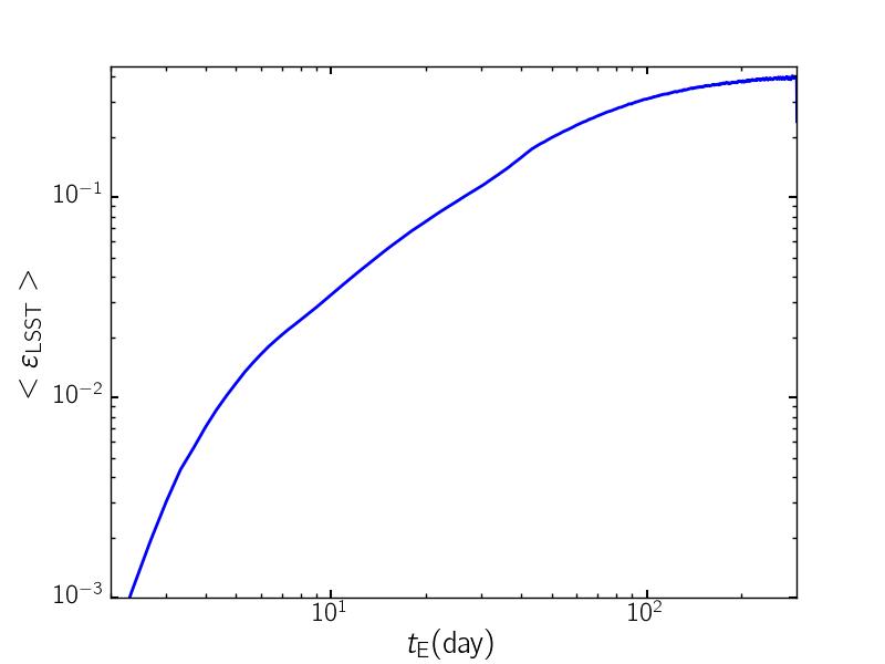
Figure 7.— The LSST efficiency for detecting microlensing event versus the Einstein crossing time which is resulted from Monte Carlo simulation.

In order to estimate the number of observable microlensing events, we evaluate the number of background and visible stars. Our criterion for visibility is that blended stellar brightness should be between LSST detection and saturation limits at least at one filter. The total number of these stars toward a given direction and per square degree is given by:

$$N_{\star,\rm{LSST}}(l,b)=\frac{2}{3}\int_{0}^{\infty}n_{t}(l,b,D_{s})\epsilon_{\rm{LSST}}(l,b,D_{s})D^{2}_{s}dD_{s},$$ (6)

where $\epsilon_{\rm{LSST}}(l,b,D_{s})$ is the efficiency for specifying stars located at a given distance toward a given direction at least at one LSST filter. We multiply $N_{\star,\rm{LSST}}$ by a factor of $2/3$ because around one third of stars are in binary systems and can not be discerned separately. Figure 6 shows the map of $N_{\star,\rm{LSST}}$ per square degree throughout the Galactic plane, which is very high toward the Galactic bulge in comparison with other directions. Because of the high extinction toward the Galactic disk ($|b|<1.5^{\circ}$) the number of visible stars reduces for these directions.

Finally, we can estimate the number of observable microlensing events per square degree during the observing time $T_{obs}$, using:

$$N_{e}(l,b)=\Gamma_{\rm{obs}}(l,b)\leavevmode\nobreak\ T_{obs}\leavevmode\nobreak\ N_{\star,\rm{LSST}}(l,b),$$ (7)

Figure 6 represents the map of $N_{e}(l,b)$ per square degree per year in the logarithmic scale. The number of microlensing events toward the Galactic bulge and disk are in the order of $400$ and $15$ per square degree, respectively. Therefore, on the average the LSST fields toward the Galactic bulge and disk the number of events will be $3840$ and $144$, respectively during $10$ years observation with the $3.9\rm{-day}$ cadence. Accordingly, LSST will detect very large number of microlensing events in comparison with the nowadays surveys because of (i) large FoV and (ii) its deep observations. Certainly, the probability of observing special events, e.g., the events with stellar black holes as microlenses, is high in large population of detected microlensing events.

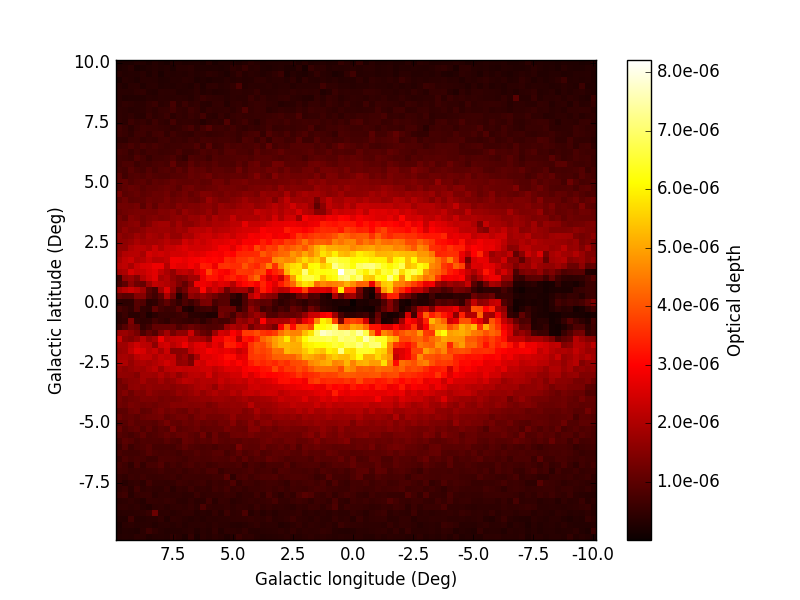
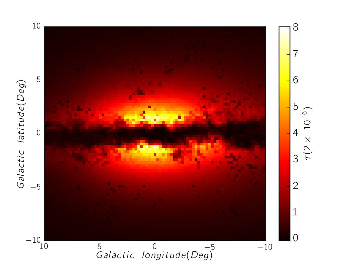
Figure 8.— Top panel: The map of the optical depth for DIA sources brighter than $23$ mag in $I$-band which was done by Manchester-Besançon Microlensing simulator(MaB$\mu$LS) (Awiphan et al., 2016). Bottom panel: The map of optical depth resulted from the simulation in this work. In order to have the same color range for both plots, we multiply the bottom map by $1/2$.

In order to quantitatively compare the detectable microlensing events toward different directions in the Galaxy, in Table (1), we report the characteristics and statistics of these events for four different directions. The first column of this table specifies the Galactic latitude and longitude of these directions. The first direction is toward Baade’s window, the second one is toward the $\beta\leavevmode\nobreak\$Sct ( which is one of four directions observed by EROS-II, the end of the Galactic bar is visible from this line of sight), other directions are toward the Galactic plane. In each row, the values of the physical parameters (first rows) and their standard deviations (second rows) calculated over the detectable microlensing events are reported. Two last columns are calculated over the area of the given line of sight, i.e., $N_{\star,l,\rm{LSST}}=N_{\star,\rm{LSST}}\times\Omega_{l}$ and $N_{e,l}=N_{e}\times\Omega_{l}$. The number of visible stars per line of sight and the blending effect toward the Galactic bulge is higher than those toward the Galactic disk. As one can expect, the optical depth toward the Galactic bulge is higher than that toward the Galactic disk which causes the high number of detectable microlensing events toward the Galactic bulge. In the next subsection, we check the validity of our simulation by comparing with other microlensing observations.

3.2. Comparison of the LSST simulation with other observations

Table 2 The effect of changing cadence on the LSST microlensing detections toward two directions with $(l=1^{\rm{\circ}},b=-4^{\rm{\circ}})$ and $(l=300^{\rm{\circ}},b=3^{\rm{\circ}})$.

$cadence$	$\log_{10}[t_{\rm{E}}]$	$v_{t}$	$u_{0}$	$f_{b}$	$m_{base,r}$	$\widetilde{\varepsilon}_{\rm{LSST}}$	$\Gamma_{\rm{obs}}(10^{-7})$	$N_{e,l}$
$\rm{(day)}$	$\rm{(day)}$	$\rm{(km\leavevmode\nobreak\ s^{-1})}$			$\rm{(mag)}$		$\rm{(star^{-1}yr^{-1})}$
				$(l=1^{\rm{\circ}},b=-4^{\rm{\circ}})$
$2.0$	$1.37$	$127.10$	$0.42$	$0.68$	$21.50$	$2.93e-3$	$21.59$	$31.18$
$3.0$	$1.40$	$122.13$	$0.43$	$0.71$	$21.33$	$2.29e-3$	$15.92$	$23.33$
$4.0$	$1.43$	$117.21$	$0.44$	$0.73$	$21.21$	$1.83e-3$	$12.51$	$18.26$
$5.0$	$1.46$	$112.81$	$0.44$	$0.74$	$21.11$	$1.49e-3$	$10.19$	$14.88$
$6.0$	$1.49$	$108.39$	$0.45$	$0.76$	$21.03$	$1.24e-3$	$8.52$	$12.17$
				$(l=300^{\circ},b=3^{\circ})$
$2.0$	$1.65$	$70.40$	$0.38$	$1.00$	$22.07$	$0.42$	$7.81$	$1.00$
$3.0$	$1.68$	$68.60$	$0.44$	$1.00$	$21.89$	$0.36$	$6.42$	$0.82$
$4.0$	$1.70$	$66.54$	$0.44$	$1.00$	$21.75$	$0.32$	$5.45$	$0.70$
$5.0$	$1.74$	$65.01$	$0.45$	$1.00$	$21.64$	$0.29$	$4.73$	$0.60$
$6.0$	$72.46$	$63.46$	$0.45$	$1.00$	$21.55$	$0.26$	$4.18$	$0.53$

The EROS-II team has searched the microlensing events toward the Galactic spiral arms, away from the Galactic bulge (Rahal et al., 2009). Moniez et al. (2017) simulated the EROS-II observations and from comparing the real observations with the simulation constrained the kinematics of the disk, the stellar mass function and the maximum contribution of a thick disk in the form of the compact objects. In order to test our code by replicating the results of EROS-II, we repeat the simulation toward the four directions of EROS-II observations with the same conditions. Also, we use the function of the EROS-II efficiency for detecting microlensing events versus the Einstein crossing time (plotted in their Figure (6)) as the detectability function. Toward $\beta\leavevmode\nobreak\$Sct with the coordinates $l=26.6^{\circ},b=-2.2^{\circ}$ we get the average value of the Einstein crossing time of $56.9$ days, which is in the agreement with the observed value of $59\pm 31$ days. The quoted uncertainty is the standard deviation from the mean value. Toward $\gamma\leavevmode\nobreak\$Sct, $l=18.5^{\circ},b=-2.1^{\circ}$, we get $<t_{\rm{E}}>=52\pm 30$ days, while the observed value was $47\pm 32$ days. Toward $\gamma\leavevmode\nobreak\$Nor with $l=331.1^{\circ},b=-2.4^{\circ}$, from simulation $<t_{\rm{E}}>=54$ days, again in the same order of the observation amount, i.e. $57$ days. Finally, toward $\theta\leavevmode\nobreak\$Mus with $l=306.6^{\circ},b=-1.5^{\circ}$ $<t_{\rm{E}}>$ from simulation and observations are $81\pm 49$ and $97$ days. The small differences between the results from our simulations and real observation are due to difference photometry systems for the source stars, their observing strategies, etc.

We also compare the optical depth map from this simulation with one resulted from Manchester-Besançon Microlensing Simulator (MaB$\mu$lS) which was developed by Awiphan et al. (2016). This simulation was based on the MOA-II observations of microlensing events. The map of the optical depth for DIA sources brighter than $23$ mag in $I$-band (the faintest limit in their simulation) from MaB$\mu$lS is shown in Figure 8 and our optical depth map in the same range of the Galactic latitude and longitude is plotted in Figure 8. These two maps are similar, but the optical depth from LSST simulation is larger than that from MaB$\mu$LS. One reason is that LSST is deeper than $23$ mag in $I$-band, even by considering the difference in their exposure times (the exposure time of MOA-II observations is $60$ seconds twice the LSST exposure which results the difference in their limiting magnitude diminishes by $\sim 0.3$ mag).

3.3. The impact of the LSST cadence on the Microlensing observation

In order to study the effect of improving the cadences on the microlensing detections with LSST, we perform the simulation with several cadences equal to $(2.0,3.0,4.0,5.0,6.0)$ days. In table (2), we report the physical parameters that depend on the cadence. These simulations are done for two directions toward (i) the Baade’s window with $(l=1^{\rm{\circ}},b=-4^{\rm{\circ}})$ and (ii) the Galactic disk with $(l=300^{\rm{\circ}},b=3^{\rm{\circ}})$. According to the table, improving the cadence makes the shorter-duration microlensing events due to somewhat fainter source stars be more observed. Since, the number of these events are intrinsically high, so by improving the cadence the number of detectable microlensing events raises. According to Table (2), changing the cadence from $6$ days to $2$ days doubles the number of observable microlensing events throughout the Galaxy.

4. LSST observing strategies

LSST is supposed to observe $449$ fields of the Galactic plane, i.e., with the coordinates $|b|<10^{\rm{\circ}}$ and $|l|<100^{\rm{\circ}}$. Each field is almost circle-shape with the diameter $3.5\leavevmode\nobreak\ \rm{deg}$ and the area $9.6\leavevmode\nobreak\ \rm{deg^{2}}$ which corresponds to $150$ lines of sight in our simulations. $178$ of these fields will be observed by LSST with the $3.9\rm{-day}$ cadence during $10$ years (I) and $271$ of these fields LSST will be observed only during the first year and with a $0.96\rm{-day}$ cadence (II). These fields are shown in Figure (9). The fields will be observed with the $3.9\rm{-day}$ cadence are represented with yellow circles and the others are shown with green ones.

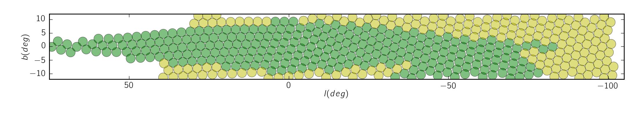
Figure 9.— The fields will be detected by LSST (I) during $10$ years with around $900$ epochs and with the averaged $3.9\rm{-day}$ cadence (yellow circles) and (II) during the first year with $30$ epochs in each filter (green circles). The area of each field is $9.6\leavevmode\nobreak\ \rm{deg^{2}}$.

Table 3 Characteristics of detectable microlensing events toward the Galactic plane with LSST by considering two different strategies (I) and (II), resulted from the Monte Carlo simulation.

	$No.\leavevmode\nobreak\ Epochs$	$No.\leavevmode\nobreak\ Fields$	$cadence$	$T_{obs}$	$<\log_{10}[t_{\rm{E}}]>$	$<u_{0}>$	$<V_{t}>$	$<f_{b,r}>$	$<A_{r}>$	$<\Gamma_{\rm{obs}}(10^{-7})>$	$N_{e,sum}$
			$\rm{(day)}$	$\rm{(yr)}$	$\rm{(day)}$		$\rm{(km\leavevmode\nobreak\ s^{-1})}$		$\rm{(mag)}$	$\rm{(star^{-1}\leavevmode\nobreak\ yr^{-1})}$
$(I)$	$900$	$178$	$3.92$	$10.0$	$1.81$	$0.44$	$79.10$	$0.94$	$1.19$	$4.28$	$7954.9$
$(II)$	$180$	$271$	$0.96$	$1.0$	$1.63$	$0.42$	$110.21$	$0.82$	$3.08$	$23.68$	$34155.3$

Note. — Averaging is done over the detectable microlensing events toward different fields. The last column is the summation number of detectable events over all related fields.

Table 4The impact of two LSST observing strategies, i.e., (I) and (II), on characteristics and statistics of detectable microlensing events toward $390$ different fields. The first column, $(l_{c},b_{c})$, indicates the coordinates of the center of each field. For other columns and for each row, two values are given which are corresponding to the strategies (I) and (II), respectively. The averaging is done over the area of each field.

$l_{c},b_{c}$	$<\log_{10}(t_{\rm{E}})>$	$<m_{base,r}>$	$<f_{b}>$	$\log_{10}[\Gamma_{\rm{obs}}(10^{7})]$	$N_{e}$	$\log_{10}[<\widetilde{\varepsilon}_{\rm{LSST}}>]$
$\rm{(deg,deg)}$	$\rm{(day)}$	$\rm{(mag)}$		$\rm{(star^{-1}yr^{-1})}$	$\rm{(deg^{-2})}$
$-99.02,-8.39$	$1.75,1.70$	$20.32,19.94$	$0.93,0.90$	$0.12,0.33$	$0.37,0.06$	$-0.20,-0.08$
$-99.53,-5.24$	$1.79,1.74$	$20.01,19.31$	$0.90,0.86$	$0.29,0.50$	$1.08,0.17$	$-0.22,-0.10$
$-99.81,+6.04$	$1.78,1.73$	$20.35,19.90$	$0.92,0.89$	$0.26,0.46$	$0.37,0.06$	$-0.21,-0.09$
$-98.14,-0.07$	$1.83,1.78$	$16.68,15.03$	$0.72,0.65$	$0.44,0.66$	$0.94,0.16$	$-0.29,-0.15$
$-98.94,+3.00$	$1.82,1.77$	$19.79,18.90$	$0.88,0.83$	$0.45,0.64$	$0.95,0.15$	$-0.23,-0.11$
$-97.44,-3.18$	$1.83,1.78$	$19.41,18.47$	$0.86,0.81$	$0.40,0.61$	$1.95,0.32$	$-0.24,-0.11$
$-97.79,+8.01$	$1.77,1.71$	$20.27,19.94$	$0.92,0.90$	$0.14,0.35$	$0.19,0.03$	$-0.20,-0.08$
$-96.35,-9.44$	$1.76,1.71$	$20.32,19.98$	$0.93,0.90$	$0.08,0.29$	$0.28,0.05$	$-0.19,-0.08$
$-96.85,-6.31$	$1.79,1.74$	$20.20,19.64$	$0.92,0.88$	$0.24,0.44$	$0.79,0.13$	$-0.21,-0.09$
$-96.10,+1.95$	$1.85,1.80$	$18.00,16.65$	$0.79,0.72$	$0.44,0.65$	$0.77,0.13$	$-0.26,-0.13$
$-96.91,+4.99$	$1.82,1.76$	$20.24,19.75$	$0.92,0.88$	$0.33,0.53$	$0.60,0.10$	$-0.20,-0.09$
$-95.36,-1.13$	$1.85,1.80$	$18.42,17.21$	$0.81,0.75$	$0.49,0.70$	$1.72,0.30$	$-0.25,-0.12$
$-95.72,+9.97$	$1.76,1.71$	$20.19,19.80$	$0.92,0.89$	$0.06,0.27$	$0.16,0.03$	$-0.19,-0.08$
$-94.15,-7.34$	$1.80,1.75$	$19.92,19.33$	$0.90,0.86$	$0.16,0.36$	$0.52,0.08$	$-0.21,-0.09$
$-94.71,-4.23$	$1.84,1.79$	$20.16,19.55$	$0.91,0.87$	$0.38,0.58$	$2.04,0.32$	$-0.20,-0.09$

Note. — A complete electronic version of this table is available at: ….

We used LSST OpSim simulations to extract epoch of observation, airmass, seeing FWHM, and filter for each visit in each field separately. These parameters have impact on the results of the simulation. We perform the Monte Carlo simulation for all of these fields to estimate the number of microlensing events that are detected by LSST by considering the corresponding their realistic strategies (I) and (II) and use the sequence of time, airmass, FWHM, filter for simulating syntectic data points for each simulated light curve. The table (3) contains the results of these simulations. The first row represents the characteristics of detectable microlensing events toward the fields shown with yellow circle in Figure (9) during $10$ years observations with the $3.9\rm{-day}$ cadence and the second row, (II), shows the properties of the detectable microlensing events toward the other fields (green circle in Figure 9).

According to this table, LSST with the second strategy (II) will detect shorter-duration events than those are detectable with the first strategy (I). According to Figure (9), most of fields with small Galactic latitude (toward the Galactic bulge and disk) will be detected with the second strategy, whereas toward these directions the optical depth is higher. Consequently, the number of detectable microlensing events with the strategy (II) during one year with the $0.96\rm{-day}$ cadence is more than those detected by the first strategy. Also, the stellar extinction for these directions is high which makes the averaged impact parameter of the detectable events be a little smaller. However, the microlensing events potentially detectable the strategy (II) will be of low value. The reasons are (i) the number of baseline data points is rare so that the source fluxes can not be estimated accurately. (ii) Lack of baseline data intensifies the degeneracy between the source flux and the Einstein crossing time which in turn causes weak estimations of the events’ timescale. During one year observation, (iii) measuring the parallax effect for long-duration microlensing events and (iv) discerning the variable stars from microlensing events are difficult. All of these issues can be solved by increasing the observational time to longer than one year.

Here, we compare these strategies in the regard of detecting microlensing events toward similar fields, by simulating detectable microlensing events. Table (4) contains some characteristic and statistic parameters of detectable microlensing events toward different fields by considering the LSST observing strategies (I) and (II) (the first and second values of each parameter are due to strategies I and II, respectively). This table can be used to optimize LSST observing strategy for disk microlensing events. As an example, when some of the fields currently scheduled for strategy (II) could be observed with strategy (I), one can select the bins of Galactic longitude and in each bin select a field for which the change of strategy would give the highest increase in $N_{e}$. We note that the ratio of $N_{e}$ values for any given field in the two strategies is less dependent on simulation details than the raw values themselves. According to this table:

• Generally, during $10$ years observation with $900$ epochs (I) LSST will detect more and on average longer microlensing events than those detectable during one year observation with $180$ epochs (II). Detecting longer microlensing events somewhat justifies the negative effect of long cadence in the observing strategy (I) on detection of short signals in microlenssing events, e.g., planetary ones. Usually, the longer microlensing events have longer planetary signals, because the time of caustic crossing is proportional to the Einstein crossing time. Hence, with the first observing strategy (I) although the time interval between data points is long and around $3.9$ days, but detectable events are on average longer and as a result have longer planetary signals.

• With the second strategy (II) the probability of detecting microlensing events is higher than that with the other, because the number of short-duration microlensing events is intrinsically higher than long-duration ones. This cause that increasing the observing time from one year to $10$ years does not enhance the number of detectable events by a factor of $10$.

• Mostly, the source stars of detectable events with the strategy (I) are somewhat fainter with higher blending effect than those with the second strategy.

Accordingly, LSST can have significant sensitivity to exoplanets throughout the Galaxy, if either if cadence better than $\sim 1-$day is executed, or follow-up observations are conducted. By detecting planets toward different directions in the Galaxy, we can study their Galactic distribution (Gould, 2013).

5. Summary and conclusions

We studied the detection of microlensing events toward the Galactic disk and bulge with LSST. In this regard, we performed a Monte Carlo simulation according to its strategy toward the Galactic longitude and latitude in the ranges of $|l|<100^{\mathrm{\circ}}$ and $|b|<10^{\mathrm{\circ}}$. We assumed that the cadence of the LSST observations is equal to $3.9$ days and its exposure time is $30$ seconds. The results of the simulation were

(i) LSST mostly detects the microlensing events of source stars with the average magnitude around $22$ in $r-$band. Although fainter stars (up to $24.3$ mag in this filter) are visible by LSST, but microlensing events due to these faint stars have small chance to be realized. Because of large blending effect they have to be highly magnified to generate high enough signal to noise ratios. But on the other hand, the high-magnification microlensing events’ durations are scaled by the lens impact parameters, i.e., their durations are mostly short in comparison to the LSST cadence.

(ii) Generally, the detectable microlensing events are (little) longer than common events observable with nowadays surveys. Thus, LSST partly helps to study microlensing events with more massive microlenses or closer events, etc.

(iii) We predicted that LSST on average detects around $400$ and $15$ microlensing events per square degree (or $3840$ and $144$ per LSST’s FoV) during its lifetime toward the Galactic bulge and disk, respectively. This large number of visible microlensing events are due to its large FoV and its observing depth.

We performed some simulations with different cadences to study the effect of cadence on the statistics and properties of observable microlensing events. Our simulations show that improving the cadence increases the detection efficiency for short-timescale events. The number of these events is intrinsically high. Therefore improving the cadence raises the number of detectable microlensing events, e.g. improving the cadence from $6$ days to $2$ days approximately doubles the number of detectable microlensing events throughout the Galaxy.

The current strategy for LSST is that it observes (I) some parts of the sky with the average $3.9\rm{-day}$ cadence during $10$ years and (II) some other parts of the sky with $180$ epochs during the first year of its lifetime. We performed the simulation by considering the corresponding strategies for these fields (shown in Figure 9) and concluded that the number of events corresponding to these strategies are $7900$ and $34000$, respectively. Most of fields with small Galactic latitude (toward the Galactic bulge and disk) are supposed to be detected with the second strategy. Toward these directions, the stellar number density and as a results the optical depth and the event rate are higher which results the larger number of detectable microlensing events.

We have also presented expected number of events for each field under both observing strategies (Table 4) which could be used to optimize the LSST observing strategy. Toward alike field, LSST with first observing strategy (I) will detect more and on average longer microlensing events than those observable with the strategy (II). Although the cadence in the first strategy is long, but on the other hand long observing time ($10$ years) helps carefully measuring the baseline source fluxes and the parallax effect for long events, discerning the variable stars from microlensing events, etc., whereas they are difficult to measure if only one year of observations is available. In addition, because of longer observing time the statistic of detectable events is higher with the first strategy than that with the second strategy.

Lastly, LSST can have significant role on detecting planets throughout the Galaxy and studying their Galactic distribution; either with the first strategy as well as follow-up observations or with the second strategy, i.e. $\sim 1-$day cadence or shorter, but with somewhat longer observing time. In addition, LSST Observation of the Galactic disk during several years with $\sim 3.9-$day cadence, first strategy (I), will allow finding isolated black holes. Long observing time helps to measure their parallax effects and baseline magnitudes, etc.

We present here Table (5) and (6) which contain the number behind the maps shown in Figure (1), (4), (5) and (6).

Table 5Properties of detectable microlensing events with LSST, resulted from Monte Carlo simulation in this work.

$b$	$l$	$filter$	$m_{base}$	$A$	$f_{b}$	$\log_{10}[N_{\rm{PSF}}]$
$\rm{(deg)}$	$\rm{(deg)}$		$\rm{(mag)}$	$\rm{(mag)}$
$-10.00$	$-100.00$	$u$	$21.69970$	$0.64350$	$0.39450$	$0.00000$
$-10.00$	$-100.00$	$g$	$22.81030$	$0.48670$	$0.90100$	$0.00000$
$-10.00$	$-100.00$	$r$	$22.34540$	$0.35430$	$0.97950$	$0.00000$
$-10.00$	$-100.00$	$i$	$21.72710$	$0.26670$	$0.99450$	$0.00000$
$-10.00$	$-100.00$	$z$	$21.15100$	$0.19060$	$0.99800$	$0.00000$
$-10.00$	$-99.75$	$u$	$21.43780$	$1.12170$	$0.40550$	$0.00000$
$-10.00$	$-99.75$	$g$	$22.71040$	$0.84760$	$0.87600$	$0.00000$
$-10.00$	$-99.75$	$r$	$22.31460$	$0.61890$	$0.96700$	$0.00000$
$-10.00$	$-99.75$	$i$	$21.67870$	$0.46510$	$0.99050$	$0.00000$
$-10.00$	$-99.75$	$z$	$21.11810$	$0.33260$	$0.99200$	$0.00000$
$-10.00$	$-99.50$	$u$	$21.80940$	$1.39950$	$0.37000$	$0.00000$
$-10.00$	$-99.50$	$g$	$22.90770$	$1.05950$	$0.85450$	$0.00000$
$-10.00$	$-99.50$	$r$	$22.50760$	$0.77520$	$0.97600$	$0.00000$
$-10.00$	$-99.50$	$i$	$21.85850$	$0.58320$	$0.99400$	$0.00000$
$-10.00$	$-99.50$	$z$	$21.24650$	$0.41770$	$0.99650$	$0.00000$

Note. — A complete electronic version of this table is available at: ….

Table 6Characteristics and statistics of detectable microlensing events with LSST by considering $3.9\rm{-day}$ cadence during $10$ years observation, resulted from the Monte Carlo simulation in this work.

$b$	$l$	$\log_{10}[\widetilde{\varepsilon}_{\rm{LSST}}]$	$t_{\rm{E}}$	$R_{\rm{E}}$	$D_{s}$	$D_{l}$	$V_{t}$	$u_{0}$	$\log_{10}[M_{t,l}]$	$\log_{10}[\Gamma_{\rm{obs}}(10^{7})]$	$\log_{10}[N_{e}]$	$\log_{10}[N_{\star,LSST}]$	$\log_{10}[\tau_{\rm{DIA}}(10^{6})]$
$\rm{(deg)}$	$\rm{(deg)}$		$\rm{(day)}$	$\rm{(A.U.)}$	$\rm{(kpc)}$	$\rm{(kpc)}$	$\rm{(km\leavevmode\nobreak\ s^{-1})}$		$\rm{(M_{\odot})}$	$\rm{(star^{-1}\leavevmode\nobreak\ yr^{-1})}$	$\rm{(deg^{-2}\leavevmode\nobreak\ yr^{-1})}$	$\rm{(deg^{-2})}$
$-10.00$	$-100.00$	$-0.32950$	$74.01988$	$1.22901$	$3.46638$	$1.15046$	$37.13148$	$0.44591$	$3.90800$	$-0.09399$	$-1.97754$	$5.11645$	$-1.46942$
$-10.00$	$-99.75$	$-0.34193$	$74.53259$	$1.23582$	$3.47254$	$1.17777$	$37.51582$	$0.45630$	$3.90986$	$-0.11888$	$-2.00431$	$5.11457$	$-1.46623$
$-10.00$	$-99.50$	$-0.35131$	$72.55770$	$1.18267$	$3.37450$	$1.13198$	$36.78578$	$0.43920$	$3.91171$	$-0.11623$	$-2.01914$	$5.09709$	$-1.47847$
$-10.00$	$-99.25$	$-0.35372$	$75.76251$	$1.21863$	$3.48016$	$1.13086$	$36.20193$	$0.43940$	$3.91358$	$-0.12951$	$-2.02424$	$5.10527$	$-1.46433$
$-10.00$	$-99.00$	$-0.31723$	$78.02045$	$1.26823$	$3.59088$	$1.19090$	$36.53486$	$0.45678$	$3.91545$	$-0.09689$	$-1.96167$	$5.13522$	$-1.44782$
$-10.00$	$-98.75$	$-0.30567$	$76.64276$	$1.24093$	$3.55187$	$1.15963$	$35.66640$	$0.45350$	$3.91732$	$-0.08422$	$-1.94408$	$5.14013$	$-1.45223$
$-10.00$	$-98.50$	$-0.32552$	$75.24845$	$1.23505$	$3.47227$	$1.15603$	$36.39649$	$0.45534$	$3.91919$	$-0.10268$	$-1.98341$	$5.11927$	$-1.46294$
$-10.00$	$-98.25$	$-0.30856$	$75.94121$	$1.23738$	$3.50554$	$1.17161$	$36.38862$	$0.46233$	$3.92107$	$-0.08374$	$-1.93576$	$5.14798$	$-1.45383$
$-10.00$	$-98.00$	$-0.31838$	$77.03021$	$1.24994$	$3.54215$	$1.16636$	$36.09435$	$0.44784$	$3.92296$	$-0.09162$	$-1.94100$	$5.15062$	$-1.44843$
$-10.00$	$-97.75$	$-0.31122$	$78.53271$	$1.25469$	$3.54835$	$1.17180$	$35.98262$	$0.44922$	$3.92485$	$-0.07587$	$-1.93779$	$5.13808$	$-1.44928$
$-10.00$	$-97.50$	$-0.30685$	$75.28133$	$1.22850$	$3.42993$	$1.15033$	$36.34997$	$0.45606$	$3.92674$	$-0.07189$	$-1.92490$	$5.14699$	$-1.46231$
$-10.00$	$-97.25$	$-0.33082$	$79.04265$	$1.20851$	$3.50570$	$1.16402$	$34.02276$	$0.45836$	$3.92864$	$-0.12090$	$-1.98132$	$5.13958$	$-1.45210$
$-10.00$	$-97.00$	$-0.31608$	$81.40951$	$1.26586$	$3.60313$	$1.19656$	$34.78856$	$0.45368$	$3.93054$	$-0.11019$	$-1.97297$	$5.13722$	$-1.44009$
$-10.00$	$-96.75$	$-0.29546$	$76.32363$	$1.22607$	$3.56775$	$1.17462$	$35.93456$	$0.45508$	$3.93245$	$-0.06069$	$-1.90376$	$5.15693$	$-1.44033$
$-10.00$	$-96.50$	$-0.31639$	$79.89724$	$1.24175$	$3.54047$	$1.16884$	$34.20550$	$0.45662$	$3.93436$	$-0.11107$	$-1.95927$	$5.15180$	$-1.44527$
$-10.00$	$-96.25$	$-0.31503$	$79.64673$	$1.23656$	$3.52473$	$1.18407$	$34.88030$	$0.45795$	$3.93628$	$-0.09068$	$-1.92447$	$5.16621$	$-1.44406$
$-10.00$	$-96.00$	$-0.29148$	$80.02194$	$1.25062$	$3.57555$	$1.20952$	$34.98413$	$0.45785$	$3.93820$	$-0.07200$	$-1.91518$	$5.15682$	$-1.43938$
$-10.00$	$-95.75$	$-0.29907$	$78.89009$	$1.23438$	$3.54191$	$1.17186$	$34.19057$	$0.44439$	$3.94012$	$-0.08367$	$-1.92138$	$5.16230$	$-1.43962$
$-10.00$	$-95.50$	$-0.30835$	$80.93421$	$1.24297$	$3.48118$	$1.13764$	$34.38667$	$0.45068$	$3.94205$	$-0.10264$	$-1.95680$	$5.14583$	$-1.44879$
$-10.00$	$-95.25$	$-0.31660$	$79.75581$	$1.24499$	$3.52980$	$1.18787$	$34.52375$	$0.45699$	$3.94398$	$-0.10362$	$-1.95656$	$5.14707$	$-1.43938$
$-10.00$	$-95.00$	$-0.34153$	$82.27132$	$1.26053$	$3.62626$	$1.19934$	$33.80105$	$0.44619$	$3.94591$	$-0.13114$	$-2.00462$	$5.12652$	$-1.42911$
$-10.00$	$-94.75$	$-0.33274$	$78.02614$	$1.20751$	$3.55568$	$1.14844$	$34.25120$	$0.45313$	$3.94785$	$-0.10777$	$-1.96562$	$5.14215$	$-1.43711$
$-10.00$	$-94.50$	$-0.33143$	$80.47062$	$1.24882$	$3.53934$	$1.16409$	$34.25127$	$0.44153$	$3.94980$	$-0.10675$	$-1.97165$	$5.13509$	$-1.43557$

Note. — A complete electronic version of this table is available at: ….

References

- Awiphan et al. (2016) Awiphan, S., Kerins, E., & Robin, A. C. 2016, MNRAS, 456, 1666
- Binney & Tremaine (2008) Binney, J., & Tremaine, S. 2008, Galactic Dynamics: Second Edition (Princeton University Press)
- Cardelli et al. (1989) Cardelli, J. A., Clayton, G. C., & Mathis, J. S. 1989, ApJ, 345, 245
- Dominik (2007) Dominik, M. 2007, MNRAS, 377, 1679
- Einstein (1936) Einstein, A. 1936, Science, 84, 506
- Fukugita et al. (1996) Fukugita, M., Ichikawa, T., Gunn, J. E., Doi, M., Shimasaku, K., & Schneider, D. P. 1996, AJ, 111, 1748
- Gould (2013) Gould, A. 2013, arXiv[astro-ph.GA]: 1304.3455
- Gwyn (2008) Gwyn, S. D. J. 2008, PASP, 120, 212
- Ivezic et al. (2009) Ivezic, Z., et al. 2009, in Bulletin of the American Astronomical Society, Vol. 41, American Astronomical Society Meeting Abstracts #213, 366
- Kayser et al. (1986) Kayser, R., Refsdal, S., & Stabell, R. 1986, A&A, 166, 36
- Kerins et al. (2009) Kerins, E., Robin, A. C., & Marshall, D. J. 2009, MNRAS, 396, 1202
- LSST Science Collaboration et al. (2017) LSST Science Collaboration et al. 2017, arXiv[astro-ph.IM]: 1708.04058
- Marshall et al. (2006) Marshall, D. J., Robin, A. C., Reylé, C., Schultheis, M., & Picaud, S. 2006, A&A, 453, 635
- Moniez et al. (2017) Moniez, M., Sajadian, S., Karami, M., Rahvar, S., & Ansari, R. 2017, A&A, 604, A124
- Mróz et al. (2017) Mróz, P., et al. 2017, Nature, 548, 183
- Nataf et al. (2013) Nataf, D. M., et al. 2013, ApJ, 769, 88
- Penny et al. (2017) Penny, M. T., Rattenbury, N. J., Gaudi, B. S., & Kerins, E. 2017, AJ, 153, 161
- Rahal et al. (2009) Rahal, Y. R., et al. 2009, A&A, 500, 1027
- Robin et al. (2012) Robin, A. C., Marshall, D. J., Schultheis, M., & Reylé, C. 2012, A&A, 538, A106
- Robin et al. (2003) Robin, A. C., Reylé, C., Derrière, S., & Picaud, S. 2003, A&A, 409, 523
- Wyrzykowski et al. (2015) Wyrzykowski, Ł., et al. 2015, ApJS, 216, 12