\stackMath

Memory effects in the Fermi-Pasta-Ulam Model

Graziano Amati1, Hugues Meyer1,2, Tanja Schilling1

1 Physikalisches Institut, Albert-Ludwigs-Universität, 79104 Freiburg, Germany
2 Unit in Engineering Science, Université du Luxembourg, L-4364 Esch-sur-Alzette, Luxembourg

Abstract

We study the Intermediate Scattering Function (ISF) of the strongly-nonlinear Fermi-Pasta Ulam Model at thermal equilibrium, using both numerical and analytical methods. From the molecular dynamics simulations we distinguish two limit regimes, as the system behaves as an ideal gas at high temperature and as a harmonic chain for low excitations. At intermediate temperatures the ISF relaxes to equilibrium in a nontrivial fashion. We then calculate analytically the Taylor coefficients of the ISF to arbitrarily high orders (the specific, simple shape of the two-body interaction allows us to derive an iterative scheme for these.) The results of the recursion are in good agreement with the numerical ones. Via an estimate of the complete series expansion of the scattering function, we can reconstruct within a certain temperature range its coarse-grained dynamics. This is governed by a memory-dependent Generalized Langevin Equation (GLE), which can be derived via projection operator techniques. Moreover, by analyzing the first series coefficients of the ISF, we can extract a parameter associated to the strength of the memory effects in the dynamics.

1 Introduction

The Fermi-Pasta-Ulam Model (FPU) consists of a one-dimensional chain of N𝑁N particles interacting through a nearest-neighbor potential. The system was at first conceived as a simple numerical tool to probe the spread of chaos in nonlinear dynamical systems. It is typically interpreted as a nonlinear crystal, while at the same time it can map a broad class of other realistic systems such as DNA structures [1] and polymer chains [2]; even the dynamics of growth models evolves according to similar differential equations in one dimension [3].
In the case of harmonic interactions the system is integrable, and it can be explicitly decoupled into independent normal modes. If a small nonlinearity is included in the interactions, the system is supposed to become chaotic. In particular, if we excite only a small fraction of modes in the initial state, we expect transport of energy to the other proper frequencies. The analysis of time scales associated to this relaxation process is an intriguing problem, which has been the topic of a scientific debate for more than 606060 years (detailed reviews can be found in [4, 5]).
The results of the very first study on the system by E. Fermi, J. Pasta, S. Ulam and M. Tsingou were published in 195519551955 [6, 7]. The authors were interested in the time needed by the system to reach equipartition from out-of-equilibrium initial conditions, in case the nonlinear dynamics was close to the integrable one. They therefore chose a two body-potential consisting of a main quadratic term, plus small higher-order corrections; they then assigned the total energy to the normal mode with the lowest frequency, and integrated numerically the equations of motion. To their surprise they found that, below a certain threshold, energy was exchanged only within a small subset of long wavelength modes. This unexpected result turned out to be in apparent contrast with the classical results from Ergodic Theory: Fermi himself in [8] tried to generalize a Poincaré theorem, which was showing how an arbitrarily small perturbation of an integrable Hamiltonian suffices to ensure equipartition of energy. An intense and fruitful debate followed, leading to the interpretation of the observations within the framework of the KAM Theorem for discrete lattices [9]. In the continuum limit the quasi-integrability behavior was shown to be related to the energy conservation of solitary waves [10]. In general, the relation between conservation laws and localization phenomena in the system turns out to be a quite involved issue [11]. Sixty year after its original formulation, the “FPU Problem” is still an open and relevant challenge for the foundation of the Dynamical Systems and Statistical Mechanics.
In the typical studies on the FPU Model, initial data are chosen very far from thermal equilibrium. However, it has been shown in [12] that the dynamics of the system can relax to metastable states even by sampling initial conditions with a large probability w.r.t. the Gibbs measure. The relevant observables in this case are the energy fluctuations, which can relax to nonequilibrium values. Other critical observables for the analysis of the system in canonical equilibrium are the energies of packets of normal modes. In [13] is has been shown how to construct an adiabatic invariant from those variables ; in [14] it is proven that localization translates into a non-exponential decay of the correlation function of those energies. The general procedure described there is based on the analysis of the poles of the Laplace transform of the correlation function. This can be estimated via the calculation of high order Lie derivatives of dynamical variables. Such quantities will also play a central role in the present work.
Another relevant issue involves the strength of the non-linearity: as the original localization has been observed in a quasi-harmonic potential, it is not obvious that Ergodicity violation can also be seen in the strongly anharmonic regime. This problem has been tackled in [15]. In this work the dynamics of the FPU chain is analyzed with highly nonlinear interactions. In this case the model can be interpreted as a glass former, as many disordered metastable basins appear in the potential landscape. For sufficiently low energy the dynamics remains trapped in one of those minima, and traces of this localization can be seen in an the anomalous relaxation of the harmonic part of the total energy.
From the discussion above, it emerges that the analysis of phase space localization and quasi-integrability in the model is strongly dependent on the choice of a few relevant observables. We can in general refer to such dimensionality reduction procedures as coarse-graining. The most general and successful formalism in this context has been developed by Mori [16] and Zwanzig [17], and extended by Grabert [18]. Within this framework one can write an exact equation of motion for the time evolution of one or few observables and the related self-time correlations. This kind of coarse-grained dynamics is governed by integro-differential equations in time, meaning that the current state of the system is history-dependent. This feature is a consequence of the fact that the Markovianity of Hamilton’s (microscopic) equations is lost due to the severe dimensionality reduction from the entire phase space of the problem to the few variables considered. The Mori-Zwanzig formalism has been widely and successfully applied in Liquid-State Theory for the analysis of scattering functions, i.e. correlations of the Fourier transforms of the density fluctuations. The strong interest behind this class of function is due to both their experimental availability and their effectiveness in capturing arrested states and glass transitions in amorphous liquids. For instance, a recursive approach for the reconstruction of the dynamic structure factor of the harmonic chain is discussed in [19]. There, an iterative method is derived in order to reconstruct systematically the infinite fraction associated to the Langevin equation of the density fluctuations in Laplace space. The analysis is based on the extraction of static recurrants related to the moments of the observable.

In the present work we analyze the dynamics of a generalization of the self-ISF in the FPU Model at equilibrium. The model and the observable are described in Section 2. In Section 3 we present and discuss the results from Molecular Dynamics (MD) simulations. In particular we show how the relaxation of the ISF is affected by the temperature of the system, and how the integrable limit of the harmonic chain can be traced at very low temperatures. In Section 4 we describe a recursive algorithm for the exact calculation of the Taylor coefficients of the ISF. Via this method we can in particular avoid the numerical errors introduced by the calculation of time derivatives from MD simulations. At the end of that section we present a comparison between different approaches for the calculations of these moments, and a discussion of their temperature dependence. Finally, in Section 5 we show how we can reconstruct for a certain temperature range the whole memory kernel of the GLE of the scattering function. The method relies on a coarse-graining procedure derived via projection operators techniques in [20]. Via the analysis of the first series coefficients we are moreover able to quantify the temperature regime associated to the observed dynamical crossover. The most technical aspects of the work have been collected in a series of appendices for the interested readers.

2 The Model

Consider a one-dimensional chain of N𝑁N identical particles with mass m𝑚m each, interacting through a nearest-neighbor non-linear potential. The Hamiltonian of the system can be written as:

H=j=0N1pj22m+j=1N1Vη(qjqj1)𝐻superscriptsubscript𝑗0𝑁1superscriptsubscript𝑝𝑗22𝑚superscriptsubscript𝑗1𝑁1subscript𝑉𝜂subscript𝑞𝑗subscript𝑞𝑗1H=\sum_{j=0}^{N-1}\frac{p_{j}^{2}}{2m}+\sum_{j=1}^{N-1}V_{\eta}(q_{j}-q_{j-1})

We set boundary conditions of Dirichlet type

q0=0,qN1=Lq_{0}=0\quad,\quad q_{N-1}=L

where the total length L𝐿L is the sum of distances between neighboring particles. We use a quartic nonlinear potential with

Vη(r)=α[(rσ)2+A(η)(rσ)3+B(η)(rσ)4]subscript𝑉𝜂𝑟𝛼delimited-[]superscript𝑟𝜎2𝐴𝜂superscript𝑟𝜎3𝐵𝜂superscript𝑟𝜎4V_{\eta}(r)=\alpha\left[\left(\frac{r}{\sigma}\right)^{2}+A(\eta)\left(\frac{r}{\sigma}\right)^{3}+B(\eta)\left(\frac{r}{\sigma}\right)^{4}\right] (1)

and coefficients

A(η)𝐴𝜂\displaystyle A(\eta) =24ηabsent24𝜂\displaystyle=-2-4\eta
B(η)𝐵𝜂\displaystyle B(\eta) =1+3ηabsent13𝜂\displaystyle=1+3\eta

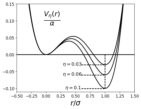
This particular parametrization of the potential has been chosen such that the positions of the two minima remain fixed while η=V(σ)/α𝜂𝑉𝜎𝛼\eta=-V(\sigma)/\alpha tunes the unbalance between their depths (see Appendix A.1).
Refer to caption
Figure 1: Shape of the two body interaction potential for three different values of the parameter η𝜂\eta

The main observable discussed in this work is the Intermediate Scattering function (ISF), constructed as follows: given the inter-particle distance between two tagged nearest neighbors rjqjqj1subscript𝑟𝑗subscript𝑞𝑗subscript𝑞𝑗1r_{j}\equiv q_{j}-q_{j-1}, we can define its spacial density as

ρj(r)=δ(rjr)superscript𝜌𝑗𝑟𝛿subscript𝑟𝑗𝑟\rho^{j}(r)=\delta(r_{j}-r)

which can be Fourier transformed into the density fluctuation

AKj=eiKrjsuperscriptsubscript𝐴𝐾𝑗superscript𝑒𝑖𝐾subscript𝑟𝑗A_{K}^{j}=e^{iKr_{j}}

The time propagation of this variable is expanded as

eiKrjeiKrj(t)=eiteiKrj=n(it)nn!eiKrjsuperscript𝑒𝑖𝐾subscript𝑟𝑗superscript𝑒𝑖𝐾subscript𝑟𝑗𝑡superscript𝑒𝑖𝑡superscript𝑒𝑖𝐾subscript𝑟𝑗subscript𝑛superscript𝑖𝑡𝑛𝑛superscript𝑒𝑖𝐾subscript𝑟𝑗e^{iKr_{j}}\rightarrow e^{iKr_{j}(t)}=e^{i\mathcal{L}t}e^{iKr_{j}}=\sum_{n}\frac{(i\mathcal{L}t)^{n}}{n!}e^{iKr_{j}} (2)

where the Liouvillian \mathcal{L} is defined as the operator acting on the phase space points 𝚪=(𝐪,𝐩)𝚪𝐪𝐩\bm{\Gamma}=(\mathbf{q},\mathbf{p}) as

i=𝚪˙𝚪=i=02N2Γ˙iΓi=i=0N1[q˙iqi+p˙ipi]𝑖bold-˙𝚪𝚪superscriptsubscript𝑖02𝑁2subscript˙Γ𝑖subscriptΓ𝑖superscriptsubscript𝑖0𝑁1delimited-[]subscript˙𝑞𝑖subscript𝑞𝑖subscript˙𝑝𝑖subscript𝑝𝑖i\mathcal{L}=\bm{\dot{\Gamma}}\cdot\frac{\partial}{\partial\mathbf{\Gamma}}=\sum_{i=0}^{2N-2}\dot{\Gamma}_{i}\frac{\partial}{\partial\Gamma_{i}}=\sum_{i=0}^{N-1}\left[\dot{q}_{i}\frac{\partial}{\partial q_{i}}+\dot{p}_{i}\frac{\partial}{\partial p_{i}}\right]

and eitsuperscript𝑒𝑖𝑡e^{i\mathcal{L}t} is the time evolution operator under Hamilton’s dynamics. The magnitude of 1/K1𝐾1/K fixes the length-scale at which we probe the system. In the following we will stick to 𝒪(1/K)𝒪(σ)similar-to𝒪1𝐾𝒪𝜎\mathcal{O}(1/K)\sim\mathcal{O}(\sigma). The time autocorrelation function of AKjsubscriptsuperscript𝐴𝑗𝐾A^{j}_{K} is defined as

Cj(t)=d𝝁[eitAKj(𝚪)]AKj(𝚪)=eiK(rj(t)rj(0))βsubscript𝐶𝑗𝑡differential-d𝝁delimited-[]superscript𝑒𝑖𝑡subscriptsuperscript𝐴𝑗𝐾𝚪superscriptsubscriptsuperscript𝐴𝑗𝐾𝚪subscriptdelimited-⟨⟩superscript𝑒𝑖𝐾subscript𝑟𝑗𝑡subscript𝑟𝑗0𝛽C_{j}(t)=\int\mathrm{d}\bm{\mu}\;\left[e^{i\mathcal{L}t}A^{j}_{K}(\bm{\Gamma})\right]{A^{j}_{K}}^{*}(\bm{\Gamma})=\left\langle e^{iK(r_{j}(t)-r_{j}(0))}\right\rangle_{\beta} (3)

where d𝝁=d𝚪ρβ(𝚪)d𝝁d𝚪subscript𝜌𝛽𝚪\mathrm{d}\bm{\mu}=\mathrm{d}\bm{\Gamma}\;\rho_{\beta}(\bm{\Gamma}) is the Gibbs measure. We omit in the notation the dependence of Cjsubscript𝐶𝑗C_{j} on the inverse temperature β𝛽\beta and the wavevector K𝐾K, not to make the notation too heavy. The series expansion of Cj(t)subscript𝐶𝑗𝑡C_{j}(t) can be naturally deduced from the Taylor series of the time evolution operator:

Cj(t)=n=0+1n![(it)neiKrj]eiKrjβ=n=0+(1)n(2n)!|(it)neiKrj|2β=n=0+t2n(2n)!ω2nsubscript𝐶𝑗𝑡superscriptsubscript𝑛01𝑛subscriptdelimited-⟨⟩delimited-[]superscript𝑖𝑡𝑛superscript𝑒𝑖𝐾subscript𝑟𝑗superscript𝑒𝑖𝐾subscript𝑟𝑗𝛽superscriptsubscript𝑛0superscript1𝑛2𝑛subscriptdelimited-⟨⟩superscriptsuperscript𝑖𝑡𝑛superscript𝑒𝑖𝐾subscript𝑟𝑗2𝛽superscriptsubscript𝑛0superscript𝑡2𝑛2𝑛subscript𝜔2𝑛C_{j}(t)=\sum_{n=0}^{+\infty}\frac{1}{n!}\left\langle\left[(i\mathcal{L}t)^{n}e^{iKr_{j}}\right]e^{-iKr_{j}}\right\rangle_{\beta}=\sum_{n=0}^{+\infty}\frac{(-1)^{n}}{(2n)!}\left\langle\lvert(i\mathcal{L}t)^{n}e^{iKr_{j}}\rvert^{2}\right\rangle_{\beta}=\sum_{n=0}^{+\infty}\frac{t^{2n}}{(2n)!}\omega_{2n} (4)

The second identity in eqn. 4 is a consequence of the anti-Hermicity of i𝑖i\mathcal{L} with respect to the scalar product induced by the canonical phase average. In the last identity we defined the coefficients

ω2nsubscript𝜔2𝑛\displaystyle\omega_{2n} [(i)2neiKrj]eiKrjβ=(1)n|(i)neiKrj|2βabsentsubscriptdelimited-⟨⟩delimited-[]superscript𝑖2𝑛superscript𝑒𝑖𝐾subscript𝑟𝑗superscript𝑒𝑖𝐾subscript𝑟𝑗𝛽superscript1𝑛subscriptdelimited-⟨⟩superscriptsuperscript𝑖𝑛superscript𝑒𝑖𝐾subscript𝑟𝑗2𝛽\displaystyle\equiv\left\langle\left[(i\mathcal{L})^{2n}e^{iKr_{j}}\right]e^{-iKr_{j}}\right\rangle_{\beta}=(-1)^{n}\left\langle\lvert(i\mathcal{L})^{n}e^{iKr_{j}}\rvert^{2}\right\rangle_{\beta} (5)
ω2n+1subscript𝜔2𝑛1\displaystyle\omega_{2n+1} 0n1absent0for-all𝑛1\displaystyle\equiv 0\;\;\;\forall n\geq 1 (6)

The knowledge of the series of these coefficients would in principle allow to reconstruct the whole dynamics of Cj(t)subscript𝐶𝑗𝑡C_{j}(t) within the convergence radius of the series in eqn. 4 (a preliminary study on the convergence domain is discussed in Appendix LABEL:cony_radius). The solution of the correlation function for an ideal gas (with a purely kinetic Hamiltonian) can be computed exactly via the knowledge of the series of the respective {ω2nid}n=0+superscriptsubscriptsubscriptsuperscript𝜔id2𝑛𝑛0\left\{\omega^{\operatorname{id}}_{2n}\right\}_{n=0}^{+\infty} (see A.2.1, eqn. A.2.1):

Cid(t)=n=0+t2n(2n)!ω2nid=1πn=0+(1)n(4K2mβ)n(2n)!π4nn!t2n(2n)!=eK2mβt2=e(tτ)2superscript𝐶id𝑡superscriptsubscript𝑛0superscript𝑡2𝑛2𝑛subscriptsuperscript𝜔id2𝑛1𝜋superscriptsubscript𝑛0superscript1𝑛superscript4superscript𝐾2𝑚𝛽𝑛2𝑛𝜋superscript4𝑛𝑛superscript𝑡2𝑛2𝑛superscript𝑒superscript𝐾2𝑚𝛽superscript𝑡2superscript𝑒superscript𝑡𝜏2C^{\operatorname{id}}(t)=\sum_{n=0}^{+\infty}\frac{t^{2n}}{(2n)!}\omega^{\operatorname{id}}_{2n}=\frac{1}{\sqrt{\pi}}\sum_{n=0}^{+\infty}(-1)^{n}\left(\frac{4K^{2}}{m\beta}\right)^{n}\frac{(2n)!\sqrt{\pi}}{4^{n}n!}\frac{t^{2n}}{(2n)!}=e^{-\frac{K^{2}}{m\beta}t^{2}}=e^{-\left(\frac{t}{\tau}\right)^{2}} (7)

where we defined the timescale

τ=mβK2𝜏𝑚𝛽superscript𝐾2\tau=\sqrt{\frac{m\beta}{K^{2}}}

that will ease the comparison of correlation functions with different values of β𝛽\beta and K𝐾K in the next section.
In case a potential term is introduced into the Hamiltonian, the dynamics is defined as mixing if the time-correlation of any couple of dynamical variables converges to its phase average:

f(t)gβfβgβ0for t+f,gL2(d𝝁)formulae-sequencesubscriptdelimited-⟨⟩𝑓𝑡superscript𝑔𝛽subscriptdelimited-⟨⟩𝑓𝛽subscriptdelimited-⟨⟩superscript𝑔𝛽0formulae-sequencefor 𝑡for-all𝑓𝑔superscript𝐿2d𝝁\left\langle f(t)g^{*}\right\rangle_{\beta}-\left\langle f\right\rangle_{\beta}\left\langle g^{*}\right\rangle_{\beta}\to 0\hskip 11.38109pt\text{for }t\to+\infty\hskip 28.45274pt\forall f,g\in L^{2}(\mathrm{d}\bm{\mu}) (8)

A mixing dynamical system is in particular ergodic. In the case of our observable, eqn. 8 reads as:

limt+C(t)j\displaystyle\lim_{t\to+\infty}C{{}_{j}}(t) =limt+eiKrj(t)(eiKrj)β=eiKrjβeiKrjβ=cos(Krj)β2+sin(Krj)β2absentsubscript𝑡subscriptdelimited-⟨⟩superscript𝑒𝑖𝐾subscript𝑟𝑗𝑡superscriptsuperscript𝑒𝑖𝐾subscript𝑟𝑗𝛽subscriptdelimited-⟨⟩superscript𝑒𝑖𝐾subscript𝑟𝑗𝛽superscriptsubscriptdelimited-⟨⟩superscript𝑒𝑖𝐾subscript𝑟𝑗𝛽superscriptsubscriptdelimited-⟨⟩𝐾subscript𝑟𝑗𝛽2superscriptsubscriptdelimited-⟨⟩𝐾subscript𝑟𝑗𝛽2\displaystyle=\lim_{t\to+\infty}\left\langle e^{iKr_{j}(t)}{\left(e^{iKr_{j}}\right)}^{*}\right\rangle_{\beta}=\left\langle e^{iKr_{j}}\right\rangle_{\beta}\left\langle e^{iKr_{j}}\right\rangle_{\beta}^{*}{\color[rgb]{0,0,1}}=\left\langle\cos(Kr_{j})\right\rangle_{\beta}^{2}+\left\langle\sin(Kr_{j})\right\rangle_{\beta}^{2}
[1Zr1(β)+drjeβVη(rj)cos(Krj)]2+[1Zr1(β)+drjeβVη(rj)sin(Krj)]2Cβsimilar-to-or-equalsabsentsuperscriptdelimited-[]1subscriptsuperscript𝑍1𝑟𝛽superscriptsubscriptdifferential-dsubscript𝑟𝑗superscript𝑒𝛽subscript𝑉𝜂subscript𝑟𝑗𝐾subscript𝑟𝑗2superscriptdelimited-[]1subscriptsuperscript𝑍1𝑟𝛽superscriptsubscriptdifferential-dsubscript𝑟𝑗superscript𝑒𝛽subscript𝑉𝜂subscript𝑟𝑗𝐾subscript𝑟𝑗2subscript𝐶𝛽\displaystyle\simeq\left[\frac{1}{Z^{1}_{r}(\beta)}\int_{-\infty}^{+\infty}\mathrm{d}r_{j}e^{-\beta V_{\eta}(r_{j})}\cos(Kr_{j})\right]^{2}+\left[\frac{1}{Z^{1}_{r}(\beta)}\int_{-\infty}^{+\infty}\mathrm{d}r_{j}e^{-\beta V_{\eta}(r_{j})}\sin(Kr_{j})\right]^{2}\equiv C_{\beta} (9)

where

Zr1(β)=+dreβVη(rj)superscriptsubscript𝑍𝑟1𝛽superscriptsubscriptdifferential-d𝑟superscript𝑒𝛽subscript𝑉𝜂subscript𝑟𝑗Z_{r}^{1}(\beta)=\int_{-\infty}^{+\infty}\mathrm{d}re^{-\beta V_{\eta}(r_{j})}

The approximation in the eqn. 2 is due to the fact that statistical independence of positions and momenta is not strictly satisfied when fixing both the ends of the chain. To simplify the estimation of the phase averages in this case we will assume that such un-entanglement applies, as it would be the case of a chain with one free end. The approximation is justified for the short-times dynamics of a tagged degree of freedom far from the boundaries, such that the finite size effects are minimized. Let us remark that within the mentioned assumption the long-time limit Cβsubscript𝐶𝛽C_{\beta} becomes independent on j𝑗j, according to eqn. 2.
For the analysis of the decay to equilibrium of a correlation function, it is convenient to subtract the long time limit from Cj(t)subscript𝐶𝑗𝑡C_{j}(t) and to define the ISF

Fj(t)Cj(t)CβCj(0)Cβsubscript𝐹𝑗𝑡subscript𝐶𝑗𝑡subscript𝐶𝛽subscript𝐶𝑗0subscript𝐶𝛽F_{j}(t)\equiv\frac{C_{j}(t)-C_{\beta}}{C_{j}(0)-C_{\beta}}

We again imply the dependence of Fjsubscript𝐹𝑗F_{j} on K𝐾K and β𝛽\beta. We note that in the kinematic regime Fid(t)=Cid(t)superscript𝐹id𝑡superscript𝐶id𝑡F^{\operatorname{id}}(t)=C^{\operatorname{id}}(t) and that all the correlation functions considered here are bounded: as AKjL2(d𝝁)subscriptsuperscript𝐴𝑗𝐾superscript𝐿2d𝝁A^{j}_{K}\in L^{2}(\mathrm{d}\bm{\mu}) we have

|AjK(t)(AjK)β|[AjK(t)(AjK(t))βAjK(AjK)β]1/2=1subscriptdelimited-⟨⟩superscriptsubscript𝐴𝑗𝐾𝑡superscriptsuperscriptsubscript𝐴𝑗𝐾𝛽superscriptdelimited-[]subscriptdelimited-⟨⟩superscriptsubscript𝐴𝑗𝐾𝑡superscriptsuperscriptsubscript𝐴𝑗𝐾𝑡𝛽subscriptdelimited-⟨⟩superscriptsubscript𝐴𝑗𝐾superscriptsuperscriptsubscript𝐴𝑗𝐾𝛽121\left\lvert\left\langle A_{j}^{K}(t)\left(A_{j}^{K}\right)^{*}\right\rangle_{\beta}\right\rvert\leq\left[\left\langle A_{j}^{K}(t)\left(A_{j}^{K}(t)\right)^{*}\right\rangle_{\beta}\left\langle A_{j}^{K}\left(A_{j}^{K}\right)^{*}\right\rangle_{\beta}\right]^{1/2}=1 (10)

as a consequence of Schwartz’s inequality.

In the next section we present a numerical study of the dynamics of the ISF. The results from the numerical simulations show a continuous temperature driven transition from ideal gas to the harmonic limit as we initialize the system in cooler states; we discuss how this phenomenology is directly related to a localization of the dynamics in the phase space.

3 Numerical Simulations

To study the time evolution of the ISF, we run molecular dynamics simulations for a chain of N=32,768𝑁32768N=32,768 particles with equal masses m=1𝑚1m=1. The parameters of the potential are set to α=9.5𝛼9.5\alpha=9.5, σ=1𝜎1\sigma=1, η=0.01𝜂0.01\eta=0.01. In all the following figures the inverse temperature is given in units of the potential scale α𝛼\alpha. The set of initial configurations is generated according to the Boltzmann distribution

ρβ(𝐫)=1Z(β)eβj=1N1Vη(rj)=1Z1N1(β)j=1N1eβVη(rj)subscript𝜌𝛽𝐫1𝑍𝛽superscript𝑒𝛽superscriptsubscript𝑗1𝑁1subscript𝑉𝜂subscript𝑟𝑗1superscriptsubscript𝑍1𝑁1𝛽superscriptsubscriptproduct𝑗1𝑁1superscript𝑒𝛽subscript𝑉𝜂subscript𝑟𝑗\rho_{\beta}(\mathbf{r})=\frac{1}{{Z(\beta)}}e^{-\beta\sum_{j=1}^{N-1}V_{\eta}(r_{j})}=\frac{1}{Z_{1}^{N-1}(\beta)}\prod_{j=1}^{N-1}e^{-\beta V_{\eta}(r_{j})}

which we factorized into single particle distributions, each associated to the same partition function

Z1(β)+dreβVη(r)subscript𝑍1𝛽superscriptsubscriptdifferential-d𝑟superscript𝑒𝛽subscript𝑉𝜂𝑟Z_{1}(\beta)\equiv\int_{-\infty}^{+\infty}\mathrm{d}re^{-\beta V_{\eta}(r)}

The initial configurations of the particles are then determined by

qj=k=0jrk,1jN1formulae-sequencesubscript𝑞𝑗superscriptsubscript𝑘0𝑗subscript𝑟𝑘1𝑗𝑁1q_{j}=\sum_{k=0}^{j}r_{k},\hskip 28.45274pt1\leq j\leq N-1

while the initial velocities are drawn from the Maxwell distribution at inverse temperature β𝛽\beta. The trajectories of the particles qjsubscript𝑞𝑗q_{j}, 1jN21𝑗𝑁21\leq j\leq N-2 are computed via the symplectic integration scheme leap-frog [21], while keeping the first and last particle of the system fixed to their initial positions q0=0,qN1=Lformulae-sequencesubscript𝑞00subscript𝑞𝑁1𝐿q_{0}=0,\;q_{N-1}=L.
The total length of the chain is a constant of motion at the trajectory level. However, expectation values w.r.t. the canonical distribution are computed by averaging over bundles of initial configurations for which the lengths L𝐿L are not identical – but due to the large size of the system they are very close to a unique function of the temperature L=L(β)𝐿𝐿𝛽L=L(\beta) .

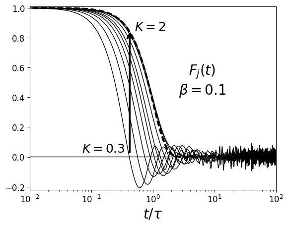
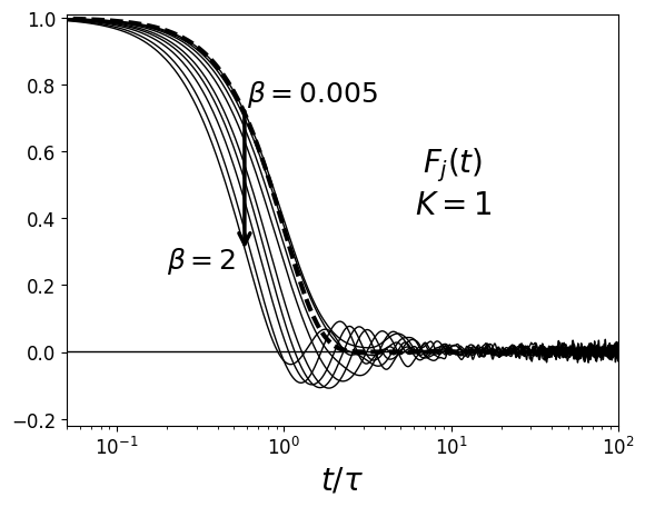
Figure 3 shows the ISF as a function of the temperature-rescaled time t/τ𝑡𝜏t/\tau; each curve corresponds to a different value of β𝛽\beta. Here and in the following graphs we show the dynamics of the central coordinate j=N2𝑗𝑁2j=\left\lfloor\frac{N}{2}\right\rfloor, the farthest from the boundaries of the system. The dotted line refers to the Gaussian relaxation in the limit of ideal gas, eqn. 7. We can see that for increasing values of β𝛽\beta all the correlations converge faster (in the rescaled time) to their equilibrium value, while preserving a Gaussian decay. Figure 3 shows the ISF for different wave vectors as a function of t/τ𝑡𝜏t/\tau. As K𝐾K is the inverse of the wavelength at which the system is probed, the system tends to equilibrate faster at smaller K𝐾K, i.e. the details of the microscopic dynamics are not probed on larger length-scales.
Refer to caption
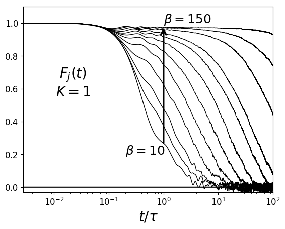
Figure 2: ISF for different values of β𝛽\beta, K=1𝐾1K=1
Refer to caption
Figure 3: ISF for different values of K𝐾K, β=0.1𝛽0.1\beta=0.1

Fig. 4 shows the time series of the ISF for values β𝛽\beta higher than the ones considered in Fig. 3. In this regime the equilibration time increases continuously for decreasing temperatures, in contrast to Fig. 3. We can interpret this process as a dynamical localization transition exhibited in the temperature range where the details of the shape of the two-body potential become relevant. The particles’ dynamics deviates from the ideal gas limit as the system becomes more and more confined to the lower potential wells. Due to energy constraints the particle’s kinetic energy is in general not sufficient for them to jump over the barrier in the two body interaction in Fig. 1. Only large fluctuations may allow this hopping process to happen, thus they occur at a vanishing rate for β+𝛽\beta\to+\infty.

Refer to caption
Figure 4: Time series of the ISF for lower temperatures than in Fig. 3 and 3. The wave vector is fixed in all the curves to K=1𝐾1K=1. As above, curves are plotted as a function of the temperature-rescaled time t/τ𝑡𝜏t/\tau.

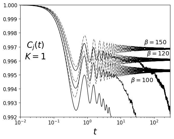
Now we focus on the time dependence of the three highest curves in Fig. 4, corresponding to the lowest temperatures considered. In Fig. 5 we compare these correlation functions with the harmonic limits for the same values of β𝛽\beta and K𝐾K (dotted lines); a semi-analytical expression for this limit is derived in Appendix A.3 by linearizing the potential around its global minimum. We note that the initial decay and the early oscillations between the analytical and numerical curves remain close for finite times; the anharmonic contributions finally drive the correlation towards their equilibrium value, in agreement with eqn. 2.
Refer to caption
Figure 5: Time series of Cjsubscript𝐶𝑗C_{j} for the lowest temperatures. Dotted line: harmonic limits of the ISF (eqn. 37).

For increasing values of β𝛽\beta, the distribution of the inter-particle distances becomes more and more localized in the global minimum of the potential in r=σ=1𝑟𝜎1r=\sigma=1 (see Fig. 1). We can quantify this temperature-driven localization by computing the probabilities

P0(β)subscript𝑃0𝛽\displaystyle P_{0}(\beta) =rcdrρβ(r)absentsuperscriptsubscriptsubscript𝑟𝑐differential-d𝑟subscript𝜌𝛽𝑟\displaystyle=\int_{-\infty}^{r_{c}}\mathrm{d}r\;\rho_{\beta}(r)
P1(β)subscript𝑃1𝛽\displaystyle P_{1}(\beta) =rc+drρβ(r)absentsuperscriptsubscriptsubscript𝑟𝑐differential-d𝑟subscript𝜌𝛽𝑟\displaystyle=\int_{r_{c}}^{+\infty}\mathrm{d}r\;\rho_{\beta}(r)

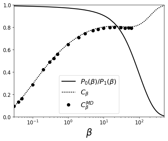
where rcsubscript𝑟𝑐r_{c} is the central local maximum in the two body potential, and of course P0(β)+P1(β)=1subscript𝑃0𝛽subscript𝑃1𝛽1P_{0}(\beta)+P_{1}(\beta)=1. We can see in Fig. 6 that the probability ratio P0/P1subscript𝑃0subscript𝑃1P_{0}/P_{1} is a monotonically decreasing function of β𝛽\beta. In the same picture are also displayed the long time limit of the correlation function Cβsubscript𝐶𝛽C_{\beta} computed with the theoretical phase average in eqn. 2 (dotted line) and by extracting the limits CβMDsubscriptsuperscript𝐶𝑀𝐷𝛽C^{MD}_{\beta} from the numerical simulations (dots). We can see that the main drop of the probability ratio happens to be the range 10β10210𝛽superscript10210\leq\beta\leq 10^{2}, in accordance with the non-monotonic behavior of Cβsubscript𝐶𝛽C_{\beta}. This temperature range corresponds to the qualitative change of behavior observed in the curves in Fig. 3 and 4.
Refer to caption
Figure 6: Solid line: probability ratio P0(β)/P1(β)subscript𝑃0𝛽subscript𝑃1𝛽P_{0}(\beta)/P_{1}(\beta); dotted line: phase average of the ISF; markers: long-time average of the ISF from the numerical simulations. We fix here the wavevector to K=1𝐾1K=1.

In this section we showed by numerical evidence that the ISF in the present generalization is a valuable tool for the analysis of the dynamics and related localization phenomena in the FPU chain. The evolution of the function is sensitive to the temperature at which the system is initialized, and a critical value β=βc10/α𝛽subscript𝛽𝑐similar-to10𝛼\beta=\beta_{c}\sim 10/\alpha could be identified as a separator between two behaviors: the fast quasi-exponential decay in Fig. 3, and a strongly non-Gaussian relaxation in Fig. 4 converging towards the harmonic limit in Fig. 5.
In the following we discuss a method for the recursive calculation of the series coefficients of the ISF. We will then use these coefficients to study the memory effects exhibited by the system.

4 Construction of the Dynamics

In this section we present an iterative method for the exact reconstruction of the ISF via the calculation of the correlators ωnsubscript𝜔𝑛\omega_{n}, as defined in eqn. 5. This approach is based on a direct evaluation of the action of (i)nsuperscript𝑖𝑛(i\mathcal{L})^{n} on the density fluctuations.
When dealing with the full microscopic dynamics, we need to choose a proper set of coordinates to keep track of the coupling between the different d.o.f., and to reduce the complexity of the many-body problem. As the potential depends only on the distances between nearest-neighbors (eqn. 1), the displacements rj=qjqj1subscript𝑟𝑗subscript𝑞𝑗subscript𝑞𝑗1r_{j}=q_{j}-q_{j-1} appear to be a natural set of configurations. One can show that πj=n=jN1pjsubscript𝜋𝑗superscriptsubscript𝑛𝑗𝑁1subscript𝑝𝑗\pi_{j}=\sum_{n=j}^{N-1}p_{j} are the conjugate momenta to these configurations. However, due to the many body sum in this expression, the calculation of phase averages of functions of πjsubscript𝜋𝑗\pi_{j}’s becomes rather involved; it is much simpler for our analytical and numerical purposes to use the non-canonical set of coordinates (𝐫,𝐩)𝐫𝐩(\mathbf{r},\mathbf{p}). As shown in Appendix A.5 that action of the Liouville operator in these coordinates is rewritten as

i𝑖\displaystyle i\mathcal{L} =i=1N1[V(ri)ri(pipi1)+1m(pipi1)ri]absentsuperscriptsubscript𝑖1𝑁1delimited-[]𝑉subscript𝑟𝑖subscript𝑟𝑖subscript𝑝𝑖subscript𝑝𝑖11𝑚subscript𝑝𝑖subscript𝑝𝑖1subscript𝑟𝑖\displaystyle=\sum_{i=1}^{N-1}\left[-\frac{\partial V(r_{i})}{\partial r_{i}}\left(\frac{\partial}{\partial p_{i}}-\frac{\partial}{\partial p_{i-1}}\right)+\frac{1}{m}\left(p_{i}-p_{i-1}\right)\frac{\partial}{\partial r_{i}}\right] (11)

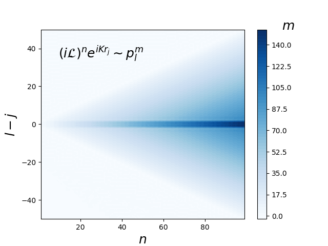
The action of the (i)nsuperscript𝑖𝑛(i\mathcal{L})^{n} on the density fluctuations can in general be written as the following complex polynomial in the coordinates

(i)neiKrjmkmin,,mkmaxslmin,,slmaxmkmin,,mkmaxslmin,,slmax(n)(rkminmkminrkmaxmkmax)(plminslminplmaxslmax)eiKrj𝐦𝐬𝐦,𝐬(n)𝐫𝐦𝐩𝐬eiKrjsuperscript𝑖𝑛superscript𝑒𝑖𝐾subscript𝑟𝑗subscriptsubscript𝑚subscript𝑘subscript𝑚subscript𝑘subscript𝑠subscript𝑙subscript𝑠subscript𝑙subscriptsuperscript𝑛subscript𝑚subscript𝑘subscript𝑚subscript𝑘subscript𝑠subscript𝑙subscript𝑠subscript𝑙superscriptsubscript𝑟subscript𝑘subscript𝑚subscript𝑘superscriptsubscript𝑟subscript𝑘subscript𝑚subscript𝑘superscriptsubscript𝑝subscript𝑙subscript𝑠subscript𝑙superscriptsubscript𝑝subscript𝑙subscript𝑠subscript𝑙superscript𝑒𝑖𝐾subscript𝑟𝑗subscript𝐦𝐬subscriptsuperscript𝑛𝐦𝐬superscript𝐫𝐦superscript𝐩𝐬superscript𝑒𝑖𝐾subscript𝑟𝑗(i\mathcal{L})^{n}e^{iKr_{j}}\equiv\sum_{\begin{subarray}{c}m_{k_{\min}},\cdots,m_{k_{\max}}\\ s_{l_{\min}},\cdots,s_{l_{\max}}\end{subarray}}\mathcal{I}^{(n)}_{\begin{subarray}{c}m_{k_{\min}},\cdots,m_{k_{\max}}\\ s_{l_{\min}},\cdots,s_{l_{\max}}\end{subarray}}\left(r_{k_{\min}}^{m_{k_{\min}}}\cdots r_{k_{\max}}^{m_{k_{\max}}}\right)\left(p_{l_{\min}}^{s_{l_{\min}}}\cdots p_{l_{\max}}^{s_{l_{\max}}}\right)e^{iKr_{j}}\equiv\sum_{\mathbf{ms}}\mathcal{I}^{(n)}_{\mathbf{m},\mathbf{s}}\mathbf{r}^{\mathbf{m}}\mathbf{p}^{\mathbf{s}}e^{iKr_{j}} (12)

with complex coefficients 𝐦𝐬(n)=𝐦𝐬(n,)+i𝐦𝐬(n,)subscriptsuperscript𝑛𝐦𝐬subscriptsuperscript𝑛𝐦𝐬𝑖subscriptsuperscript𝑛𝐦𝐬\mathcal{I}^{(n)}_{\mathbf{ms}}=\mathcal{I}^{(n,\Re)}_{\mathbf{ms}}+i\mathcal{I}^{(n,\Im)}_{\mathbf{ms}}. It would be computationally difficult to tackle eqn. 12 in case all the degrees of freedom of the system entered in the expansion at any order, i.e. if the sum ran over 𝒪(2N)𝒪2𝑁\mathcal{O}(2N) indexes. Conveniently, the interaction at the lowest orders in n𝑛n is restricted to a relatively small subset of coordinates around the tagged j𝑗j-th degree of freedom. This is a direct consequence of the nearest-neighbor nature of the interaction. In the following we will formalize this observation. From the expansion of (i)neiKrjsuperscript𝑖𝑛superscript𝑒𝑖𝐾subscript𝑟𝑗(i\mathcal{L})^{n}e^{iKr_{j}} we can identify relevant products of differentials that control the propagation of the interaction from rjsubscript𝑟𝑗r_{j} to any other d.o.f. of the chain; we will refer to these contributions as spreading operators. Via these cross derivatives we can perform a systematic study of the extent of the non-locality as a function of the order n𝑛n. For example, the composition of derivatives connecting the configuration rjsubscript𝑟𝑗r_{j} of the tagged particle to another generic coordinate rksubscript𝑟𝑘r_{k} located on the right (R) of rjsubscript𝑟𝑗r_{j} (k>j𝑘𝑗k>j) is given by

σrR(n,j,kj)θ(n2k+j)[(Vrk)(pkpk1)]θ(n2)×\displaystyle{\sigma_{r}^{R}}(n,j,k-j)\equiv\theta\left(\left\lfloor\frac{n}{2}\right\rfloor-k+j\right)\left[\left(-\frac{\partial V}{\partial r_{k}}\right)\left(\frac{\partial}{\partial p_{k}}-\frac{\partial}{\partial p_{k-1}}\right)\right]^{\theta(n-2)}\times
×{i=0kj2[1m(pj+i+1pj+i)rj+i+1][(Vrj+i+1)(pj+i+1pj+i)]}θ(n4)[1m(pjpj1)rj]θ(n2)absentsuperscriptsuperscriptsubscriptproduct𝑖0𝑘𝑗2delimited-[]1𝑚subscript𝑝𝑗𝑖1subscript𝑝𝑗𝑖subscript𝑟𝑗𝑖1delimited-[]𝑉subscript𝑟𝑗𝑖1subscript𝑝𝑗𝑖1subscript𝑝𝑗𝑖𝜃𝑛4superscriptdelimited-[]1𝑚subscript𝑝𝑗subscript𝑝𝑗1subscript𝑟𝑗𝜃𝑛2\displaystyle\times\left\{\prod_{i=0}^{k-j-2}\left[\frac{1}{m}(p_{j+i+1}-p_{j+i})\frac{\partial}{\partial r_{j+i+1}}\right]\left[\left(-\frac{\partial V}{\partial r_{j+i+1}}\right)\left(\frac{\partial}{\partial p_{j+i+1}}-\frac{\partial}{\partial p_{j+i}}\right)\right]\right\}^{\theta\left(n-4\right)}\left[\frac{1}{m}(p_{j}-p_{j-1})\frac{\partial}{\partial r_{j}}\right]^{\theta\left(n-2\right)} (13)

where

θ(x)={1,x00,x<0𝜃𝑥cases1𝑥00𝑥0\theta(x)=\begin{cases}1,&x\geq 0\\ 0,&x<0\end{cases}

Fox fixed n𝑛n and j𝑗j, the prefactor θ(n2k+j)𝜃𝑛2𝑘𝑗\theta\left(\left\lfloor\frac{n}{2}\right\rfloor-k+j\right) reduces the effective domain of σrRsuperscriptsubscript𝜎𝑟𝑅\sigma_{r}^{R} to the subset of coordinates that enter in (i)neiKrjsuperscript𝑖𝑛superscript𝑒𝑖𝐾subscript𝑟𝑗(i\mathcal{L})^{n}e^{iKr_{j}} i.e., that participate in the propagation of the density fluctuations at order n𝑛n. In Appendix A.6 we show the symmetric structure of σrLsubscriptsuperscript𝜎𝐿𝑟\sigma^{L}_{r}, connecting rjsubscript𝑟𝑗r_{j} to another coordinate rksubscript𝑟𝑘r_{k} on the left (L)𝐿(L) of j𝑗j (k<j𝑘𝑗k<j), as well as the expressions of the analogous operators for the momenta σp(L/R)superscriptsubscript𝜎𝑝𝐿𝑅{\sigma_{p}^{(L/R)}}. Via the spreading operators it becomes straightforward to list the subset of neighboring distances entering the interaction at order n𝑛n:

Kr(n,j)subscript𝐾𝑟𝑛𝑗\displaystyle K_{r}(n,j) {jn2,,j+n2}(2n2+1){kmin,,kmax}absent𝑗𝑛2𝑗𝑛2superscript2𝑛21subscript𝑘subscript𝑘\displaystyle\equiv\left\{j-\left\lfloor\frac{n}{2}\right\rfloor,\cdots,j+\left\lfloor\frac{n}{2}\right\rfloor\right\}\in\mathbb{N}^{\left(2\left\lfloor\frac{n}{2}\right\rfloor+1\right)}\equiv\left\{k_{\min},\cdots,k_{\max}\right\} (14)

An analogous set for the momenta are given in eqn. 49. The boundaries of the sums in eqn. 12 can again be determined identifying of the relevant differential operators of (i)nsuperscript𝑖𝑛(i\mathcal{L})^{n}. We can define r(n,j,|jk|)subscript𝑟𝑛𝑗𝑗𝑘\mathcal{M}_{r}(n,j,\lvert j-k\rvert) and 𝒮p(n,j,|jl|)subscript𝒮𝑝𝑛𝑗𝑗𝑙\mathcal{S}_{p}(n,j,\lvert j-l\rvert) as the leading power respectively for a configuration rksubscript𝑟𝑘r_{k} and a momentum plsubscript𝑝𝑙p_{l} in the sum. In vector notation these definitions read as:

𝐦=(mkminmkmax)(r(n,j,jkmin)r(n,j,kmaxj))𝐌𝐦matrixsubscript𝑚subscript𝑘subscript𝑚subscript𝑘matrixsubscript𝑟𝑛𝑗𝑗subscript𝑘subscript𝑟𝑛𝑗subscript𝑘𝑗𝐌\mathbf{m}=\begin{pmatrix}m_{k_{\min}}\\ \vdots\\ m_{k_{\max}}\\ \end{pmatrix}\leq\begin{pmatrix}\mathcal{M}_{r}(n,j,j-k_{\min})\\ \vdots\\ \mathcal{M}_{r}(n,j,k_{\max}-j)\end{pmatrix}\equiv\mathbf{M}

and analogously for the momenta

𝐬=(slminslmax)(𝒮p(n,j,jlmin)𝒮p(n,j,lmaxj))𝐒𝐬matrixsubscript𝑠subscript𝑙subscript𝑠subscript𝑙matrixsubscript𝒮𝑝𝑛𝑗𝑗subscript𝑙subscript𝒮𝑝𝑛𝑗subscript𝑙𝑗𝐒\mathbf{s}=\begin{pmatrix}s_{l_{\min}}\\ \vdots\\ s_{l_{\max}}\end{pmatrix}\leq\begin{pmatrix}\mathcal{S}_{p}(n,j,j-l_{\min})\\ \vdots\\ \mathcal{S}_{p}(n,j,l_{\max}-j)\end{pmatrix}\equiv\mathbf{S}

The boundaries of the sums in equation eqn. 12 are therefore fixed to

(i)neiKrj=𝟎𝐦𝐌𝟎𝐬𝐒𝐦𝐬(n)𝐫𝐦𝐩𝐬eiKrj[pn(𝐫,𝐩)+ipn(𝐫,𝐩)]eiKrjsuperscript𝑖𝑛superscript𝑒𝑖𝐾subscript𝑟𝑗subscript0𝐦𝐌0𝐬𝐒subscriptsuperscript𝑛𝐦𝐬superscript𝐫𝐦superscript𝐩𝐬superscript𝑒𝑖𝐾subscript𝑟𝑗delimited-[]superscriptsubscript𝑝𝑛𝐫𝐩𝑖superscriptsubscript𝑝𝑛𝐫𝐩superscript𝑒𝑖𝐾subscript𝑟𝑗\displaystyle(i\mathcal{L})^{n}e^{iKr_{j}}=\sum_{\begin{subarray}{c}\mathbf{0}\leq\mathbf{m}\leq\mathbf{M}\\ \mathbf{0}\leq\mathbf{s}\leq\mathbf{S}\end{subarray}}\mathcal{I}^{(n)}_{\mathbf{ms}}\mathbf{r^{m}p^{s}}e^{iKr_{j}}\equiv\left[p_{n}^{\Re}(\mathbf{r},\mathbf{p})+ip_{n}^{\Im}(\mathbf{r},\mathbf{p})\right]e^{iKr_{j}} (15)

where we additionally split the real and imaginary part of the polynomial expansion in the terms pn(𝐫,𝐩)superscriptsubscript𝑝𝑛𝐫𝐩p_{n}^{\Re}(\mathbf{r},\mathbf{p}) and pn(𝐫,𝐩)superscriptsubscript𝑝𝑛𝐫𝐩p_{n}^{\Im}(\mathbf{r},\mathbf{p}). By computing the averages over the Gibbs distribution we obtain as a the final expression of the Taylor coefficients

ω2nsubscript𝜔2𝑛\displaystyle\omega_{2n} =(1)n|(i)neiKrj|2β=(1)n|pn(𝐫,𝐩)+ipn(𝐫,𝐩)|2β=(1)n[(pn(𝐫,𝐩))2β+(pn(𝐫,𝐩))2β]=absentsuperscript1𝑛subscriptdelimited-⟨⟩superscriptsuperscript𝑖𝑛superscript𝑒𝑖𝐾subscript𝑟𝑗2𝛽superscript1𝑛subscriptdelimited-⟨⟩superscriptsuperscriptsubscript𝑝𝑛𝐫𝐩𝑖superscriptsubscript𝑝𝑛𝐫𝐩2𝛽superscript1𝑛delimited-[]subscriptdelimited-⟨⟩superscriptsuperscriptsubscript𝑝𝑛𝐫𝐩2𝛽subscriptdelimited-⟨⟩superscriptsuperscriptsubscript𝑝𝑛𝐫𝐩2𝛽absent\displaystyle=(-1)^{n}\left\langle\lvert(i\mathcal{L})^{n}e^{iKr_{j}}\rvert^{2}\right\rangle_{\beta}=(-1)^{n}\left\langle\lvert p_{n}^{\Re}(\mathbf{r},\mathbf{p})+ip_{n}^{\Im}(\mathbf{r},\mathbf{p})\rvert^{2}\right\rangle_{\beta}=(-1)^{n}\left[\left\langle(p_{n}^{\Re}(\mathbf{r},\mathbf{p}))^{2}\right\rangle_{\beta}+\left\langle(p_{n}^{\Im}(\mathbf{r},\mathbf{p}))^{2}\right\rangle_{\beta}\right]=
=(1)n𝟎𝐦,𝐦𝐌𝟎𝐬,𝐬𝐒(𝐦𝐬(n,)𝐦𝐬(n,)+𝐦𝐬(n,)𝐦𝐬(n,))𝐫𝐦+𝐦𝐩𝐬+𝐬βabsentsuperscript1𝑛subscriptformulae-sequence0𝐦superscript𝐦𝐌formulae-sequence0𝐬superscript𝐬𝐒subscriptsuperscript𝑛𝐦𝐬subscriptsuperscript𝑛superscript𝐦superscript𝐬subscriptsuperscript𝑛𝐦𝐬subscriptsuperscript𝑛superscript𝐦superscript𝐬subscriptdelimited-⟨⟩superscript𝐫𝐦superscript𝐦superscript𝐩𝐬superscript𝐬𝛽\displaystyle=(-1)^{n}\sum_{\begin{subarray}{c}\mathbf{0}\leq\mathbf{m,m^{\prime}}\leq\mathbf{M}\\ \mathbf{0}\leq\mathbf{s,s^{\prime}}\leq\mathbf{S}\end{subarray}}\left(\mathcal{I}^{(n,\Re)}_{\mathbf{ms}}\mathcal{I}^{(n,\Re)}_{\mathbf{m^{\prime}s^{\prime}}}+\mathcal{I}^{(n,\Im)}_{\mathbf{ms}}\mathcal{I}^{(n,\Im)}_{\mathbf{m^{\prime}s^{\prime}}}\right)\left\langle\mathbf{r^{m+m^{\prime}}p^{s+s^{\prime}}}\right\rangle_{\beta} (16)

Note that, as a consequence of the assumption of stationarity, knowledge of the n𝑛n-th order tensor of coefficients (n)superscript𝑛\mathcal{I}^{(n)} suffices to calculate ω2nsubscript𝜔2𝑛\omega_{2n}. We present now a recursive method to compute the entries of (n)superscript𝑛\mathcal{I}^{(n)}. We can extract a relation (n)(n+1)superscript𝑛superscript𝑛1\mathcal{I}^{(n)}\rightarrow\mathcal{I}^{(n+1)} directly from the action of the powers of i𝑖i\mathcal{L} on the dynamical variable:

(i)n+1eiKrj=𝟎𝐦𝐌𝟎𝐬𝐒𝐦𝐬(n+1)𝐫𝐦𝐩𝐬eiKrj=(i)(i)neiKrj=i(𝟎𝐦𝐌𝟎𝐬𝐒𝐦𝐬(n)𝐫𝐦𝐩𝐬eiKrj)superscript𝑖𝑛1superscript𝑒𝑖𝐾subscript𝑟𝑗subscript0𝐦𝐌0𝐬𝐒subscriptsuperscript𝑛1𝐦𝐬superscript𝐫𝐦superscript𝐩𝐬superscript𝑒𝑖𝐾subscript𝑟𝑗𝑖superscript𝑖𝑛superscript𝑒𝑖𝐾subscript𝑟𝑗𝑖subscript0𝐦𝐌0𝐬𝐒subscriptsuperscript𝑛𝐦𝐬superscript𝐫𝐦superscript𝐩𝐬superscript𝑒𝑖𝐾subscript𝑟𝑗\displaystyle(i\mathcal{L})^{n+1}e^{iKr_{j}}=\sum_{\begin{subarray}{c}\mathbf{0}\leq\mathbf{m}\leq\mathbf{M}\\ \mathbf{0}\leq\mathbf{s}\leq\mathbf{S}\end{subarray}}\mathcal{I}^{(n+1)}_{\mathbf{ms}}\mathbf{r^{m}p^{s}}e^{iKr_{j}}=(i\mathcal{L})(i\mathcal{L})^{n}e^{iKr_{j}}=i\mathcal{L}\left(\sum_{\begin{subarray}{c}\mathbf{0}\leq\mathbf{m}\leq\mathbf{M}\\ \mathbf{0}\leq\mathbf{s}\leq\mathbf{S}\end{subarray}}\mathcal{I}^{(n)}_{\mathbf{ms}}\mathbf{r^{m}p^{s}}e^{iKr_{j}}\right)

As an example, we can isolate from i𝑖i\mathcal{L} the contribution of

ipγV(rγ)rγ(pγpγ1)=ασ2(2rγ+3A(η)rγ2σ+4B(η)rγ3σ2)(pγpγ1)𝑖superscriptsubscript𝑝𝛾𝑉subscript𝑟𝛾subscript𝑟𝛾subscript𝑝𝛾subscript𝑝𝛾1𝛼superscript𝜎22subscript𝑟𝛾3𝐴𝜂superscriptsubscript𝑟𝛾2𝜎4𝐵𝜂superscriptsubscript𝑟𝛾3superscript𝜎2subscript𝑝𝛾subscript𝑝𝛾1i\mathcal{L}_{p}^{\gamma}\equiv-\frac{\partial V(r_{\gamma})}{\partial r_{\gamma}}\left(\frac{\partial}{\partial p_{\gamma}}-\frac{\partial}{\partial p_{\gamma-1}}\right)=-\frac{\alpha}{\sigma^{2}}\left(2r_{\gamma}+3A(\eta)\frac{r_{\gamma}^{2}}{\sigma}+4B(\eta)\frac{r_{\gamma}^{3}}{\sigma^{2}}\right)\left(\frac{\partial}{\partial p_{\gamma}}-\frac{\partial}{\partial p_{\gamma-1}}\right)

with kminγkmaxsubscript𝑘𝛾subscript𝑘k_{\min}\leq\gamma\leq k_{\max} and lmin+1γlmaxsubscript𝑙1𝛾subscript𝑙l_{\min}+1\leq\gamma\leq l_{\max} (see eqn. 49). We can then determine explicitly its action on the monomials in the expansion at order n𝑛n:

ipγ[(rkminmkminrγmγrkmaxmkmax)(plminslminpγ1sγ1pγsγplmaxslmax)]=𝑖superscriptsubscript𝑝𝛾delimited-[]superscriptsubscript𝑟subscript𝑘subscript𝑚subscript𝑘superscriptsubscript𝑟𝛾subscript𝑚𝛾superscriptsubscript𝑟subscript𝑘subscript𝑚subscript𝑘superscriptsubscript𝑝subscript𝑙subscript𝑠subscript𝑙superscriptsubscript𝑝𝛾1subscript𝑠𝛾1superscriptsubscript𝑝𝛾subscript𝑠𝛾superscriptsubscript𝑝subscript𝑙subscript𝑠subscript𝑙absent\displaystyle i\mathcal{L}_{p}^{\gamma}\left[\left(r_{k_{\min}}^{m_{k_{\min}}}\cdots r_{\gamma}^{m_{\gamma}}\cdots r_{k_{\max}}^{m_{k_{\max}}}\right)\left(p_{l_{\min}}^{s_{l_{\min}}}\cdots p_{\gamma-1}^{s_{\gamma-1}}p_{\gamma}^{s_{\gamma}}\cdots p_{l_{\max}}^{s_{l_{\max}}}\right)\right]=
=ασ2[2rγ+3A(η)rγ2σ+4B(η)rγ3σ2](pγpγ1)[(rkminmkminrγmγrkmaxmkmax)(plminslminpγ1sγ1pγsγplmaxslmax)]=absent𝛼superscript𝜎2delimited-[]2subscript𝑟𝛾3𝐴𝜂superscriptsubscript𝑟𝛾2𝜎4𝐵𝜂superscriptsubscript𝑟𝛾3superscript𝜎2subscript𝑝𝛾subscript𝑝𝛾1delimited-[]superscriptsubscript𝑟subscript𝑘subscript𝑚subscript𝑘superscriptsubscript𝑟𝛾subscript𝑚𝛾superscriptsubscript𝑟subscript𝑘subscript𝑚subscript𝑘superscriptsubscript𝑝subscript𝑙subscript𝑠subscript𝑙superscriptsubscript𝑝𝛾1subscript𝑠𝛾1superscriptsubscript𝑝𝛾subscript𝑠𝛾superscriptsubscript𝑝subscript𝑙subscript𝑠subscript𝑙absent\displaystyle=-\frac{\alpha}{\sigma^{2}}\left[2r_{\gamma}+3A(\eta)\frac{r_{\gamma}^{2}}{\sigma}+4B(\eta)\frac{r_{\gamma}^{3}}{\sigma^{2}}\right]\left(\frac{\partial}{\partial p_{\gamma}}-\frac{\partial}{\partial p_{\gamma-1}}\right)\left[\left(r_{k_{\min}}^{m_{k_{\min}}}\cdots r_{\gamma}^{m_{\gamma}}\cdots r_{k_{\max}}^{m_{k_{\max}}}\right)\left(p_{l_{\min}}^{s_{l_{\min}}}\cdots p_{\gamma-1}^{s_{\gamma-1}}p_{\gamma}^{s_{\gamma}}\cdots p_{l_{\max}}^{s_{l_{\max}}}\right)\right]=
=ασ2[rkminmkmin(2rγmγ+1+3A(η)rγmγ+2σ+4B(η)rγmγ+3σ2)rkmaxmkmax][plminslmin(pγ1sγ1sγpγsγ1sγ1pγ1sγ11pγsγ)plmaxslmax]absent𝛼superscript𝜎2delimited-[]superscriptsubscript𝑟subscript𝑘subscript𝑚subscript𝑘2superscriptsubscript𝑟𝛾subscript𝑚𝛾13𝐴𝜂superscriptsubscript𝑟𝛾subscript𝑚𝛾2𝜎4𝐵𝜂superscriptsubscript𝑟𝛾subscript𝑚𝛾3superscript𝜎2superscriptsubscript𝑟subscript𝑘subscript𝑚subscript𝑘delimited-[]superscriptsubscript𝑝subscript𝑙subscript𝑠subscript𝑙superscriptsubscript𝑝𝛾1subscript𝑠𝛾1subscript𝑠𝛾superscriptsubscript𝑝𝛾subscript𝑠𝛾1subscript𝑠𝛾1superscriptsubscript𝑝𝛾1subscript𝑠𝛾11superscriptsubscript𝑝𝛾subscript𝑠𝛾superscriptsubscript𝑝subscript𝑙subscript𝑠subscript𝑙\displaystyle=-\frac{\alpha}{\sigma^{2}}\left[r_{k_{\min}}^{m_{k_{\min}}}\cdots\left(2r_{\gamma}^{m_{\gamma}+1}+3A(\eta)\frac{r_{\gamma}^{m_{\gamma}+2}}{\sigma}+4B(\eta)\frac{r_{\gamma}^{m_{\gamma}+3}}{\sigma^{2}}\right)\cdots r_{k_{\max}}^{m_{k_{\max}}}\right]\left[p_{l_{\min}}^{s_{l_{\min}}}\cdots\left(p_{\gamma-1}^{s_{\gamma-1}}s_{\gamma}p_{\gamma}^{s_{\gamma}-1}-s_{\gamma-1}p_{\gamma-1}^{s_{\gamma-1}-1}p_{\gamma}^{s_{\gamma}}\right)\cdots p_{l_{\max}}^{s_{l_{\max}}}\right]

The contribution of ipγ𝑖superscriptsubscript𝑝𝛾i\mathcal{L}_{p}^{\gamma} to 𝐦𝐬(n+1)subscriptsuperscript𝑛1𝐦𝐬\mathcal{I}^{(n+1)}_{\mathbf{ms}} is then given by

𝐦,𝐬(n+1)|p,γαk=0,1(1)k+1sγk[2σ2𝐦+𝐞^γ,𝐬𝐞^γk(n)+3σ3A(η)𝐦+2𝐞^γ,𝐬𝐞^γk(n)+4σ4B(η)𝐦+3𝐞^γ,𝐬𝐞^γk(n)]evaluated-atsubscriptsuperscript𝑛1𝐦𝐬𝑝𝛾𝛼subscript𝑘01superscript1𝑘1subscript𝑠𝛾𝑘delimited-[]2superscript𝜎2subscriptsuperscript𝑛𝐦subscript^𝐞𝛾𝐬subscript^𝐞𝛾𝑘3superscript𝜎3𝐴𝜂subscriptsuperscript𝑛𝐦2subscript^𝐞𝛾𝐬subscript^𝐞𝛾𝑘4superscript𝜎4𝐵𝜂subscriptsuperscript𝑛𝐦3subscript^𝐞𝛾𝐬subscript^𝐞𝛾𝑘{\mathcal{I}}^{(n+1)}_{\mathbf{m,s}}\Big{|}_{p,\gamma}\equiv\alpha\sum_{k=0,1}(-1)^{k+1}s_{\gamma-k}\left[\frac{2}{\sigma^{2}}\mathcal{I}^{(n)}_{\mathbf{m}+\mathbf{\hat{e}}_{\gamma},\mathbf{s}-\mathbf{\hat{e}}_{\gamma-k}}+\frac{3}{\sigma^{3}}A(\eta)\mathcal{I}^{(n)}_{\mathbf{m}+2\mathbf{\hat{e}}_{\gamma},\mathbf{s}-\mathbf{\hat{e}}_{\gamma-k}}+\frac{4}{\sigma^{4}}B(\eta)\mathcal{I}^{(n)}_{\mathbf{m}+3\mathbf{\hat{e}}_{\gamma},\mathbf{s}-\mathbf{\hat{e}}_{\gamma-k}}\right] (17)

where the unit vectors 𝐞jsubscript𝐞𝑗\mathbf{e}_{j} are defined via their action on vectors in any dimension nsuperscript𝑛\mathbb{R}^{n} such that:

𝐯+α𝐞j={v1,,vj+α,,vn},cformulae-sequence𝐯𝛼subscript𝐞𝑗subscript𝑣1subscript𝑣𝑗𝛼subscript𝑣𝑛for-all𝑐\mathbf{v}+\alpha\mathbf{e}_{j}=\left\{v_{1},\cdots,v_{j}+\alpha,\cdots,v_{n}\right\},\hskip 14.22636pt\forall c\in\mathbb{R}

The other terms of the recursion relation are derived in Appendix A.7, while in Appendix A.11 we present a general method for the numerical management of high dimensional tensors as the ones considered in the procedure.

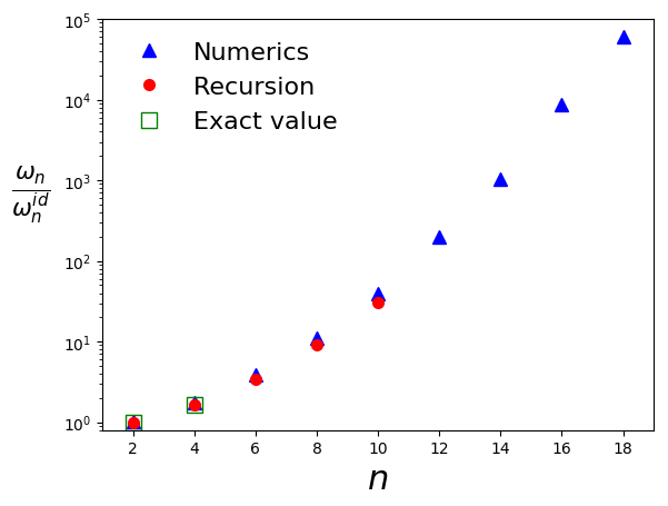
In Fig. 7 we show the dynamical correlators computed with different methods, normalized by the analytically known values of the ideal gas (eqn. A.2.1). The numerical coefficients are determined by the calculation of high order time derivatives in the trajectories of the density fluctuation, according to

ω2nMDd2ndt2neiKrj(t)|t=0eiKrjβsuperscriptsubscript𝜔2𝑛𝑀𝐷subscriptdelimited-⟨⟩evaluated-atsuperscriptd2𝑛dsuperscript𝑡2𝑛superscript𝑒𝑖𝐾subscript𝑟𝑗𝑡𝑡0superscript𝑒𝑖𝐾subscript𝑟𝑗𝛽\omega_{2n}^{MD}\equiv\left\langle\left.\frac{\mathrm{d}^{2n}}{\mathrm{d}t^{2n}}e^{iKr_{j}(t)}\right|_{t=0}e^{-iKr_{j}}\right\rangle_{\beta}

We observe optimal agreement between the recursive approach and the numerical values. The magnitude of ω2subscript𝜔2\omega_{2} is the same in the kinematic and the dynamic regime (and is therefore analytically known); the analytical value of ω4subscript𝜔4\omega_{4} in presence of nonlinearities is computed in the Appendix A.2.2.
Refer to caption
Figure 7: ωn/ωnidsubscript𝜔𝑛superscriptsubscript𝜔𝑛id\omega_{n}/\omega_{n}^{\operatorname{id}} from the MD simulations (triangles) and via the recursion relation derived in the work (circles); comparison with the analytical result for n=2,4𝑛24n=2,4 (see A.2.2); we fix to β=0.1𝛽0.1\beta=0.1, K=1𝐾1K=1.

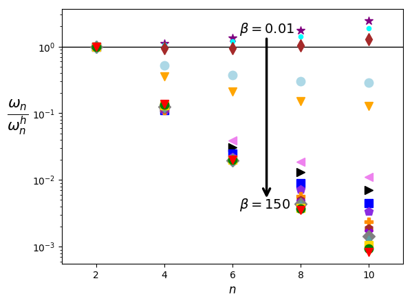
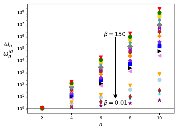
In Fig. 9 we show the sequence of the series coefficients computed via the recursion relation, for a wide range of inverse temperatures. We notice for decreasing values of β𝛽\beta a convergence of the sequences to the ideal limit. In Fig. 9 we present the same series of coefficients ωnsubscript𝜔𝑛\omega_{n} normalized w.r.t. the correspondent values computed in the harmonic limit ωnhsuperscriptsubscript𝜔𝑛\omega_{n}^{h}. The convergence of the ratios to unity is not as neat as in the previous case. We ascribe the discrepancy to the fact that a few approximations enter the semi-analytical estimate of the harmonic limit of the ISF, as discussed in Appendix A.3; in particular the system is far from its continuum limit.
Refer to caption
Figure 8: ωn/ωnidsubscript𝜔𝑛superscriptsubscript𝜔𝑛id\omega_{n}/\omega_{n}^{\operatorname{id}} for different values of β𝛽\beta and K=1𝐾1K=1
Refer to caption
Figure 9: ωn/ωnhsubscript𝜔𝑛superscriptsubscript𝜔𝑛\omega_{n}/\omega_{n}^{h} for different values of β𝛽\beta and K=1𝐾1K=1

Via the procedure presented in this section it is possible to compute the first orders of the dynamics of the ISF exactly; higher order Taylor coefficients could be computed with increasing complexity by computer algebra. Instead of pushing in this direction, in the next section we will describe a combined numerical and analytical approach that will enable us to study the dynamics of the ISF with no need of additional effort in the compuations. We will in particular determine the memory effects encapsulated in the evolution of this relevant correlation function.

5 The Generalized Langevin Equation

The dynamics of the non normalized ISF at equilibrium is governed by the GLE

dCj(t)dt=0tdtKj(tt)Cj(t)dsubscript𝐶𝑗𝑡d𝑡superscriptsubscript0𝑡differential-dsuperscript𝑡subscript𝐾𝑗𝑡superscript𝑡subscript𝐶𝑗superscript𝑡\frac{\mathrm{d}C_{j}(t)}{\mathrm{d}t}=\int_{0}^{t}\mathrm{d}t^{\prime}K_{j}(t-t^{\prime})C_{j}(t^{\prime}) (18)

which can be derived via projection operator techniques [22]. The memory kernel Kjsubscript𝐾𝑗K_{j} controls to which extent the state of the process at a certain instant in time depends on the previous evolution. In the Markovian (memory-less) limit Kj(t)=γδ(t),γ+formulae-sequencesubscript𝐾𝑗𝑡𝛾𝛿𝑡𝛾superscriptK_{j}(t)=-\gamma\delta(t),\;\gamma\in\mathbb{R}^{+}, i.e. the solution of eqn. 18 decays exponentially. We can see from the results of Section 333 that the dynamics of the ISF is far from exponential; it is therefore nontrivial to reconstruct the shape of Kjsubscript𝐾𝑗K_{j}. In this section we recover the whole time series of the kernel for a certain range of temperatures and we define a criterion to quantify the “strength of the memory”.

Following [20] and [23], we can reconstruct systematically the memory of the process via a relation between the series coefficients of the kernel

κn(ddt)nK(t)|t=0subscript𝜅𝑛evaluated-atsuperscriptdd𝑡𝑛𝐾𝑡𝑡0\kappa_{n}\equiv\left(\left.\frac{\mathrm{d}}{\mathrm{d}t}\right)^{n}K(t)\right|_{t=0}

and the ωnsubscript𝜔𝑛\omega_{n} defined in eqn. 5. This correspondence for processes at equilibrium can be implicitly written as

κn=n(ω0,ω2,,ωn+2)subscript𝜅𝑛subscript𝑛subscript𝜔0subscript𝜔2subscript𝜔𝑛2\kappa_{n}=\mathcal{F}_{n}(\omega_{0},\omega_{2},\cdots,\omega_{n+2}) (19)

being nsubscript𝑛\mathcal{F}_{n} a nonlinear combination of its arguments.
The reconstruction of Kjsubscript𝐾𝑗K_{j} from its series expansion is reduced to the calculation of its even series coefficients, as the odd ones are identically null at equilibrium. This can be easily shown by inverting tt𝑡𝑡t\rightarrow-t and ttsuperscript𝑡superscript𝑡t^{\prime}\rightarrow-t^{\prime} in eqn. 18 and noticing that as Cjsubscript𝐶𝑗C_{j} is even it follows Kj(tt)=Kj(tt)subscript𝐾𝑗𝑡superscript𝑡subscript𝐾𝑗superscript𝑡𝑡K_{j}(t-t^{\prime})=K_{j}(t^{\prime}-t); this means that the series expansion of Kjsubscript𝐾𝑗K_{j} must only include even contributions.

The reconstruction of the time series of the kernel via eqn. 19, requires the knowledge of the high-order series coefficients of C(t)jC{{}_{j}}(t). The calculation of these terms can be simplified by introducing an interpolating approximation for the correlation function CjIC(+)subscriptsuperscript𝐶𝐼𝑗superscript𝐶superscriptC^{I}_{j}\in C^{\infty}(\mathbb{R}^{+}), such that its derivatives in t=0𝑡0t=0 provide an estimate of the required Taylor coefficients. To determine a proper functional expression for the interpolating function we can proceed as follows. We can see from the main plot in Figure 3 that for sufficiently high temperatures (for β2less-than-or-similar-to𝛽2\beta\lesssim 2) the initial decay of Fj(t)subscript𝐹𝑗𝑡F_{j}(t) preserves the Gaussian shape of the ideal gas (eqn. 7). It appears therefore convenient in this low-β𝛽\beta regime to define as ansatz:

CjI(t)superscriptsubscript𝐶𝑗𝐼𝑡\displaystyle C_{j}^{I}(t) (1Cβ)eat2+Cβabsent1subscript𝐶𝛽superscript𝑒𝑎superscript𝑡2subscript𝐶𝛽\displaystyle\equiv(1-C_{\beta})e^{-at^{2}}+C_{\beta} (20)

where the superscript I𝐼I stands for “interpolation”. The long time limit Cβsubscript𝐶𝛽C_{\beta} is fixed by eqn. 2, while the Gaussian parameter a=a(β)𝑎𝑎𝛽a=a(\beta) can be extracted from the time series of Cj(t)subscript𝐶𝑗𝑡C_{j}(t) in the numerical simulations:

a=12(Cβ1)d2Cj(t)dt|t=0𝑎evaluated-at12subscript𝐶𝛽1superscriptd2subscript𝐶𝑗𝑡d𝑡𝑡0a=\frac{1}{2(C_{\beta}-1)}\left.\frac{\mathrm{d}^{2}C_{j}(t)}{\mathrm{d}t}\right|_{t=0} (21)

Via eqn. 21 we can quantify the deviation from time-temperature superposition in presence of the interaction. (At this level of description we explicitly choose to neglect the oscillatory patterns exhibited in the curves in Figures 3 and 3 before the final relaxation; we can interpret these as traces at finite temperature of the harmonic dynamics of the ISF, according to eqn. 37).

Let us remark that the shape of the ansatz in eqn. 20 is compliant with the requirement that the odd series coefficients of the ISF are identically null. We recall from eqn. 4 that this restriction is a direct consequence of the property of anti-Hermicity of the i𝑖i\mathcal{L} at equilibrium. An interpolation of the ISF with a general stretched exponential

f(t)=(1A)eBtα+A,α2formulae-sequence𝑓𝑡1𝐴superscript𝑒𝐵superscript𝑡𝛼𝐴𝛼2f(t)=(1-A)e^{Bt^{\alpha}}+A,\hskip 14.22636pt\alpha\neq 2 (22)

would violate this symmetry. These functions are frequently used to fit slowly decaying correlations [24]. The applicability of the ansatz in eqn. 22 is however restricted to regimes where the Liouville operator \mathcal{L} is not Hermitian, as it happens in general out-of-equilibrium processes.

With the ansatz eqn. 20 we can compute at any order the Taylor coefficients of CjIsubscriptsuperscript𝐶𝐼𝑗C^{I}_{j}:

ω2nIsubscriptsuperscript𝜔𝐼2𝑛\displaystyle\omega^{I}_{2n} d2nC(t)Ijdt2n|t=0=(1Cβ)an(dd(at))2ne(at)2|t=0+δn,0Cβ=\displaystyle\equiv\left.\frac{\mathrm{d}^{2n}C{{}^{I}}_{j}(t)}{\mathrm{d}t^{2n}}\right|_{t=0}=(1-C_{\beta})a^{n}\left.\left(\frac{\mathrm{d}}{\mathrm{d}(\sqrt{a}t)}\right)^{2n}e^{-(\sqrt{a}t)^{2}}\right|_{t=0}+\delta_{n,0}C_{\beta}=
=(1Cβ)an(1)2nH2n(at)e(at)2|t=0+δn,0Cβ=(1Cβ)anH2n+δn,0Cβabsentevaluated-at1subscript𝐶𝛽superscript𝑎𝑛superscript12𝑛subscript𝐻2𝑛𝑎𝑡superscript𝑒superscript𝑎𝑡2𝑡0subscript𝛿𝑛0subscript𝐶𝛽1subscript𝐶𝛽superscript𝑎𝑛subscript𝐻2𝑛subscript𝛿𝑛0subscript𝐶𝛽\displaystyle=\left.(1-C_{\beta})a^{n}(-1)^{2n}H_{2n}(\sqrt{a}t)e^{-(\sqrt{a}t)^{2}}\right|_{t=0}+\delta_{n,0}C_{\beta}=(1-C_{\beta})a^{n}H_{2n}+\delta_{n,0}C_{\beta} (23)

where we introduced Hn(x)subscript𝐻𝑛𝑥H_{n}(x), the n𝑛n-th Hermite polynomials, and the Hermite numbers HnHn(0)subscript𝐻𝑛subscript𝐻𝑛0H_{n}\equiv H_{n}(0). From the recursion relation Hn+1(x)=2xHn(x)2nHn1(x)subscript𝐻𝑛1𝑥2𝑥subscript𝐻𝑛𝑥2𝑛subscript𝐻𝑛1𝑥H_{n+1}(x)=2xH_{n}(x)-2nH_{n-1}(x) and the initial conditions H0(0)=1,H1(0)=0formulae-sequencesubscript𝐻001subscript𝐻100H_{0}(0)=1,H_{1}(0)=0, we can write the closed form

Hn={(2)n/2(n1)!!n even0n oddsubscript𝐻𝑛casessuperscript2𝑛2double-factorial𝑛1n even0n odd\displaystyle H_{n}=\begin{cases}(-2)^{n/2}(n-1)!!&\text{n even}\\ 0&\text{n odd}\end{cases}

We can insert the estimates of eqn. 23 into eqn. 19 to compute the Taylor coefficients κnIsuperscriptsubscript𝜅𝑛𝐼\kappa_{n}^{I} of the memory kernel KjIsuperscriptsubscript𝐾𝑗𝐼K_{j}^{I} for n40less-than-or-similar-to𝑛40n\lesssim 40. Above this order, the calculation of the exact expression of nsubscript𝑛\mathcal{F}_{n} become computationally expensive, due to the increasing combinatory complexity. A simplification is possible according to the theoretical arguments in Appendix A.9, where we show how that for higher orders of n𝑛n we can approximate

κ2nIω2n+2In40formulae-sequencesimilar-to-or-equalssubscriptsuperscript𝜅𝐼2𝑛subscriptsuperscript𝜔𝐼2𝑛2greater-than-or-equivalent-to𝑛40\kappa^{I}_{2n}\simeq\omega^{I}_{2n+2}\hskip 28.45274ptn\gtrsim 40 (24)

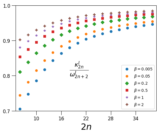
This estimate is also confirmed numerically from the convergence to unity of the ratio κ2nI/ω2n+2Isubscriptsuperscript𝜅𝐼2𝑛subscriptsuperscript𝜔𝐼2𝑛2\kappa^{I}_{2n}/\omega^{I}_{2n+2}, as shown in Fig. 10.

Refer to caption
Figure 10: Ratio κ2nI/ωn+2Isubscriptsuperscript𝜅𝐼2𝑛subscriptsuperscript𝜔𝐼𝑛2\kappa^{I}_{2n}/\omega^{I}_{n+2} as a function of n𝑛n, for different values of the inverse temperature β𝛽\beta

With this additional approximation we can now compute the short-time expansion the kernel

KjI,Nmax(tt)n=0Nmaxκ2nI(2n)!(tt)2nsuperscriptsubscript𝐾𝑗𝐼subscript𝑁𝑡superscript𝑡superscriptsubscript𝑛0subscript𝑁subscriptsuperscript𝜅𝐼2𝑛2𝑛superscript𝑡superscript𝑡2𝑛K_{j}^{I,N_{\max}}(t-t^{\prime})\equiv\sum_{n=0}^{N_{\max}}\frac{\kappa^{I}_{2n}}{(2n)!}(t-t^{\prime})^{2n} (25)

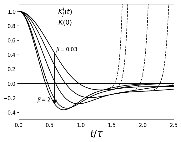
till order Nmax=180subscript𝑁180N_{\max}=180. The results for KjI,Nmaxsuperscriptsubscript𝐾𝑗𝐼subscript𝑁K_{j}^{I,N_{\max}} at different values of β𝛽\beta correspond to the first decays and the (dotted) long-time divergent lines in Fig. 11. An estimate of the convergent decay at long time is derived in Appendix A.10.
Refer to caption
Figure 11: Reconstruction of the memory kernel of the GLE (eqn. 18) for different values of β𝛽\beta and K=1𝐾1K=1, as a function of the rescaled time τ𝜏\tau. The plot of the bare expression in eqn. 25 diverges at finite times (dashed lines); the extrapolation of the convergent limits (thick lines at long times) is discussed in Appendix A.10.

In the following we would like to define a criterion to quantify the memory effects at different temperatures, and to relate them to results from the MD simulation in Section 3. We can make a direct comparison between the timescales of the ISF and the one of the related kernel by expanding these two functions as second order:

Fj(t)subscript𝐹𝑗𝑡\displaystyle F_{j}(t) =11Cβ[n=0+ω2n(2n)!t2nCβ]11Cβ[n=0+(1)n(tτ2nC)2nCβ]=1(tτ2C)2+absent11subscript𝐶𝛽delimited-[]superscriptsubscript𝑛0subscript𝜔2𝑛2𝑛superscript𝑡2𝑛subscript𝐶𝛽11subscript𝐶𝛽delimited-[]superscriptsubscript𝑛0superscript1𝑛superscript𝑡superscriptsubscript𝜏2𝑛𝐶2𝑛subscript𝐶𝛽1superscript𝑡superscriptsubscript𝜏2𝐶2\displaystyle=\frac{1}{1-C_{\beta}}\left[\sum_{n=0}^{+\infty}\frac{\omega_{2n}}{(2n)!}t^{2n}-C_{\beta}\right]\equiv\frac{1}{1-C_{\beta}}\left[\sum_{n=0}^{+\infty}(-1)^{n}\left(\frac{t}{\tau_{2n}^{C}}\right)^{2n}-C_{\beta}\right]=1-\left(\frac{t}{\tau_{2}^{C}}\right)^{2}+\cdots
Kj(t)Kj(0)subscript𝐾𝑗𝑡subscript𝐾𝑗0\displaystyle\frac{K_{j}(t)}{K_{j}(0)} =1Kj(0)n=0+κ2n(2n)!t2nn=0+(1)n(tτ2nK)2n=1(tτ2K)2+absent1subscript𝐾𝑗0superscriptsubscript𝑛0subscript𝜅2𝑛2𝑛superscript𝑡2𝑛superscriptsubscript𝑛0superscript1𝑛superscript𝑡superscriptsubscript𝜏2𝑛𝐾2𝑛1superscript𝑡superscriptsubscript𝜏2𝐾2\displaystyle=\frac{1}{K_{j}(0)}\sum_{n=0}^{+\infty}\frac{\kappa_{2n}}{(2n)!}t^{2n}\equiv\sum_{n=0}^{+\infty}(-1)^{n}\left(\frac{t}{\tau_{2n}^{K}}\right)^{2n}=1-\left(\frac{t}{\tau_{2}^{K}}\right)^{2}+\cdots

The parabolic approximation of Fjsubscript𝐹𝑗F_{j} and Kjsubscript𝐾𝑗K_{j} vanish respectively at the instants

τ2F=|2(1Cβ)ω2|τ2K=|2ω2ω4ω22|formulae-sequencesuperscriptsubscript𝜏2𝐹21subscript𝐶𝛽subscript𝜔2superscriptsubscript𝜏2𝐾2subscript𝜔2subscript𝜔4superscriptsubscript𝜔22\tau_{2}^{F}=\sqrt{\left\lvert\frac{2(1-C_{\beta})}{\omega_{2}}\right\rvert}\hskip 22.76219pt\tau_{2}^{K}=\sqrt{\left\lvert\frac{2\omega_{2}}{\omega_{4}-\omega_{2}^{2}}\right\rvert}

We can therefore define the dimensionless ratio

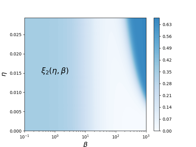
ξ2=ξ2(β,η)(τ2Kτ2F)2=11Cβω22ω4ω22subscript𝜉2subscript𝜉2𝛽𝜂superscriptsuperscriptsubscript𝜏2𝐾superscriptsubscript𝜏2𝐹211subscript𝐶𝛽superscriptsubscript𝜔22subscript𝜔4superscriptsubscript𝜔22\xi_{2}=\xi_{2}(\beta,\eta)\equiv\left(\frac{\tau_{2}^{K}}{\tau_{2}^{F}}\right)^{2}=\frac{1}{1-C_{\beta}}\frac{\omega_{2}^{2}}{\omega_{4}-\omega_{2}^{2}}

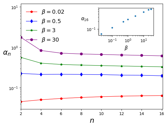
quantifying the extent of the timescale of the memory kernel w.r.t. the one of the correlation. This function of β𝛽\beta and η𝜂\eta is plotted in Fig. 12. In the limit β0𝛽0\beta\to 0 the curve approaches its limit value for an ideal gas; in particular via eqn. A.2.1 we get limβ0ξ2(β,η)=1/2subscript𝛽0subscript𝜉2𝛽𝜂12\lim_{\beta\to 0}\xi_{2}(\beta,\eta)=1/2. We can see a steady increase of the timescale by both fixing η𝜂\eta wile increasing β𝛽\beta and viceversa. We can interpret the result as follows: the strength of the memory effects increases either by decreasing the temperature or by increasing the depth of the potential well in Fig. 1. Both cases correspond to a higher localization of the system in the neighborhood of the lowest minimum of the energy landscape.
Refer to caption
Figure 12: ξ2subscript𝜉2\xi_{2} for different values of β𝛽\beta and η𝜂\eta, K=1𝐾1K=1

6 Conclusions

In this work we presented a coarse-grained analysis of the FPU Model at equilibrium, based on the numerical and analytical study of a generalization of the intermediate scattering function (ISF). Based on MD simulations it is possible to distinguish a crossover from an ideal gas regime to the integrable limit by progressively cooling the system in the initial state. We then treated analytically the sequence of the Taylor coefficients of the ISF for a wide range of temperatures. Moreover, we presented an analysis of the memory effects in the system, based on the reconstruction of the Generalized Langevin equation which governs the dynamics of the ISF. A quantitative description of the time extent of the memory is possible for a wide range of system parameters. The analysis supports the interpretation of the behavior encountered as a temperature-driven localization on phase space.
The study we presented involves several conceptual tools which are largely used in the framework of Liquid State Theory, and applied them to a model traditionally studied in the context of Dynamical Systems. The methods we empolyed can be in general extended to any observable in the system, as e.g. the normal mode energies or other relevant variables. This would allow to merge the present discussion with the problem of anomalous transport of energy between modes or the propagation of solitary waves, for different initial conditions. The hope of the authors is that, by joining the different approaches some light can be shed on the intriguing and rich phenomenology exhibited by an apparently simple system still able to question the foundations of Statistical Mechanics.

Appendix A Appendix

A.1 Two body potential

In this section we derive the expression for the two-well interaction potential between nearest neighbors used (eqn. 1). We would like to fix a parametrization in terms of a global energy scale α𝛼\alpha, a length scale σ𝜎\sigma and a factor controlling the unbalance between two wells. Therefore we can define

V(r)=α[(rσ)2+A(rσ)3+B(rσ)4]𝑉𝑟𝛼delimited-[]superscript𝑟𝜎2𝐴superscript𝑟𝜎3𝐵superscript𝑟𝜎4V(r)=\alpha\left[\left(\frac{r}{\sigma}\right)^{2}+A\left(\frac{r}{\sigma}\right)^{3}+B\left(\frac{r}{\sigma}\right)^{4}\right]

We then require that the distance r=σ𝑟𝜎r=\sigma corresponds to an equilibrium position, and we impose V(σ)ϵ𝑉𝜎italic-ϵV(\sigma)\equiv-\epsilon, ϵitalic-ϵ\epsilon\in\mathbb{R}:

dV(r)dr|r=σevaluated-atd𝑉𝑟d𝑟𝑟𝜎\displaystyle\frac{\mathrm{d}V(r)}{\mathrm{d}r}\Bigr{|}_{r=\sigma} =0=ασ[2+3A+4B]absent0𝛼𝜎delimited-[]23𝐴4𝐵\displaystyle=0=\frac{\alpha}{\sigma}\left[2+3A+4B\right]
V(σ)𝑉𝜎\displaystyle V(\sigma) =ϵ=α[1+A+B]absentitalic-ϵ𝛼delimited-[]1𝐴𝐵\displaystyle=-\epsilon=\alpha[1+A+B]

The relations are solved by

A𝐴\displaystyle A =A(η)=24ηabsent𝐴𝜂24𝜂\displaystyle=A(\eta)=-2-4\eta
B𝐵\displaystyle B =B(η)=1+3ηabsent𝐵𝜂13𝜂\displaystyle=B(\eta)=1+3\eta

With the dimensionless parameter η=ϵα𝜂italic-ϵ𝛼\eta=\frac{\epsilon}{\alpha} assuming positive values in case the minimum in r=σ𝑟𝜎r=\sigma is negative.

A.2 Analytical expression for ωnsubscript𝜔𝑛\omega_{n}

In this appendix we present the analytical expressions of the series coefficients ωnsubscript𝜔𝑛\omega_{n}; while an exact solution is easily determined at any order in the ideal gas regime, a general expression is not available in case a nonlinear interaction is added to the dynamics. For the non-integrable regime, we can still derive the analytical solution of the lowest orders; in particular in A.2.2 we compute exactly ω4subscript𝜔4\omega_{4}, which is the first coefficient that depends on the dynamics.

A.2.1 Ideal gas regime

By expanding the kinetic part of the Liouvillian (eqn. 11) in the general expression in eqn. 5 we get:

ωnidsuperscriptsubscript𝜔𝑛id\displaystyle\omega_{n}^{\operatorname{id}} =[(1mγ=1N2(pγpγ1)rγ)neiKrj]eiKrjβ=(iKm)n(pjpj1)nβ=(iKm)nk=0n(nk)pjkβ(pj1)nkβ=absentsubscriptdelimited-⟨⟩delimited-[]superscript1𝑚superscriptsubscript𝛾1𝑁2subscript𝑝𝛾subscript𝑝𝛾1subscript𝑟𝛾𝑛superscript𝑒𝑖𝐾subscript𝑟𝑗superscript𝑒𝑖𝐾subscript𝑟𝑗𝛽superscript𝑖𝐾𝑚𝑛subscriptdelimited-⟨⟩superscriptsubscript𝑝𝑗subscript𝑝𝑗1𝑛𝛽superscript𝑖𝐾𝑚𝑛superscriptsubscript𝑘0𝑛binomial𝑛𝑘subscriptdelimited-⟨⟩superscriptsubscript𝑝𝑗𝑘𝛽subscriptdelimited-⟨⟩superscriptsubscript𝑝𝑗1𝑛𝑘𝛽absent\displaystyle=\left\langle\left[\left(\frac{1}{m}\sum_{\gamma=1}^{N-2}(p_{\gamma}-p_{\gamma-1})\frac{\partial}{\partial r_{\gamma}}\right)^{n}e^{iKr_{j}}\right]e^{-iKr_{j}}\right\rangle_{\beta}=\left(\frac{iK}{m}\right)^{n}\left\langle(p_{j}-p_{j-1})^{n}\right\rangle_{\beta}=\left(\frac{iK}{m}\right)^{n}\sum_{k=0}^{n}\binom{n}{k}\left\langle p_{j}^{k}\right\rangle_{\beta}\left\langle(-p_{j-1})^{n-k}\right\rangle_{\beta}=
1π(β2m)(iKm)nk=0n(nk)(1)nk[+dpjeβpj22mpjk][+dpj1eβpj122mpj1nk]=similar-to-or-equalsabsent1𝜋𝛽2𝑚superscript𝑖𝐾𝑚𝑛superscriptsubscript𝑘0𝑛binomial𝑛𝑘superscript1𝑛𝑘delimited-[]superscriptsubscriptdifferential-dsubscript𝑝𝑗superscript𝑒𝛽superscriptsubscript𝑝𝑗22𝑚superscriptsubscript𝑝𝑗𝑘delimited-[]superscriptsubscriptdifferential-dsubscript𝑝𝑗1superscript𝑒𝛽superscriptsubscript𝑝𝑗122𝑚superscriptsubscript𝑝𝑗1𝑛𝑘absent\displaystyle\simeq\frac{1}{\pi}\left(\frac{\beta}{2m}\right)\left(\frac{iK}{m}\right)^{n}\sum_{k=0}^{n}\binom{n}{k}(-1)^{n-k}\left[\int_{-\infty}^{+\infty}\mathrm{d}p_{j}\;e^{-\beta\frac{p_{j}^{2}}{2m}}p_{j}^{k}\right]\left[\int_{-\infty}^{+\infty}\mathrm{d}p_{j-1}\;e^{-\beta\frac{p_{j-1}^{2}}{2m}}p_{j-1}^{n-k}\right]=
=1π(β2m)(iKm)n(1)n+12k=0n2(n2k)(2mβ)k+12[+dxex2x2k]×\displaystyle=\frac{1}{\pi}\left(\frac{\beta}{2m}\right)\left(\frac{iK}{m}\right)^{n}\frac{(-1)^{n}+1}{2}\sum_{k=0}^{\frac{n}{2}}\binom{n}{2k}\left(\frac{2m}{\beta}\right)^{k+\frac{1}{2}}\left[\int_{-\infty}^{+\infty}\mathrm{d}x\;e^{-x^{2}}x^{2k}\right]\times
×(2mβ)n+12k[+dxex2xn2k]=\displaystyle\times\left(\frac{2m}{\beta}\right)^{\frac{n+1}{2}-k}\left[\int_{-\infty}^{+\infty}\mathrm{d}x\;e^{-x^{2}}x^{n-2k}\right]=
=1π(β2m)(iKm)n(1)n+12(2mβ)n2+1[k=0n2(n2k)Γ(k+12)Γ(n2k+12)]=absent1𝜋𝛽2𝑚superscript𝑖𝐾𝑚𝑛superscript1𝑛12superscript2𝑚𝛽𝑛21delimited-[]superscriptsubscript𝑘0𝑛2binomial𝑛2𝑘Γ𝑘12Γ𝑛2𝑘12absent\displaystyle=\frac{1}{\pi}\left(\frac{\beta}{2m}\right)\left(\frac{iK}{m}\right)^{n}\frac{(-1)^{n}+1}{2}\left(\frac{2m}{\beta}\right)^{\frac{n}{2}+1}\left[\sum_{k=0}^{\frac{n}{2}}\binom{n}{2k}\Gamma\left(k+\frac{1}{2}\right)\Gamma\left(\frac{n}{2}-k+\frac{1}{2}\right)\right]=
=1π(1)n2(2K2mβ)n2(1)n+12π2n2Γ(n+12)=1π(1)n2(4K2mβ)n2(1)n+12Γ(n+12)absent1𝜋superscript1𝑛2superscript2superscript𝐾2𝑚𝛽𝑛2superscript1𝑛12𝜋superscript2𝑛2Γ𝑛121𝜋superscript1𝑛2superscript4superscript𝐾2𝑚𝛽𝑛2superscript1𝑛12Γ𝑛12\displaystyle=\frac{1}{\pi}(-1)^{\frac{n}{2}}\left(\frac{2K^{2}}{m\beta}\right)^{\frac{n}{2}}\frac{(-1)^{n}+1}{2}\sqrt{\pi}2^{\frac{n}{2}}\Gamma\left(\frac{n+1}{2}\right)=\frac{1}{\sqrt{\pi}}(-1)^{\frac{n}{2}}\left(\frac{4K^{2}}{m\beta}\right)^{\frac{n}{2}}\frac{(-1)^{n}+1}{2}\Gamma\left(\frac{n+1}{2}\right) (26)

where we used

pjmβ=(2mβ)m21π(1)m+12Γ(m+12)subscriptdelimited-⟨⟩superscriptsubscript𝑝𝑗𝑚𝛽superscript2𝑚𝛽𝑚21𝜋superscript1𝑚12Γ𝑚12\left\langle p_{j}^{m}\right\rangle_{\beta}=\left(\frac{2m}{\beta}\right)^{\frac{m}{2}}\frac{1}{\sqrt{\pi}}\frac{(-1)^{m}+1}{2}\Gamma\left(\frac{m+1}{2}\right)

and

k=0n2(n2k)Γ(k+12)Γ(n2k+12)=k=0n2n!(2k)!(n2k)!π(2k)!4kk!π(n2k)!4n2k(n2k)!superscriptsubscript𝑘0𝑛2binomial𝑛2𝑘Γ𝑘12Γ𝑛2𝑘12superscriptsubscript𝑘0𝑛2𝑛2𝑘𝑛2𝑘𝜋2𝑘superscript4𝑘𝑘𝜋𝑛2𝑘superscript4𝑛2𝑘𝑛2𝑘\displaystyle\sum_{k=0}^{\frac{n}{2}}\binom{n}{2k}\Gamma\left(k+\frac{1}{2}\right)\Gamma\left(\frac{n}{2}-k+\frac{1}{2}\right)=\sum_{k=0}^{\frac{n}{2}}\frac{n!}{(2k)!(n-2k)!}\cdot\sqrt{\pi}\,\frac{(2k)!}{4^{k}k!}\cdot\sqrt{\pi}\,\frac{(n-2k)!}{4^{\frac{n}{2}-k}\left(\frac{n}{2}-k\right)!}
=πn!4n2(n2)!k=0n2(n2)!k!(n2k)!=πn!4n2(n2)!k=0n2(n2k)=πn!4n2(n2)!2n2=π2n2πn!4n/2(n2)!=π2n2Γ(n+12)absent𝜋𝑛superscript4𝑛2𝑛2superscriptsubscript𝑘0𝑛2𝑛2𝑘𝑛2𝑘𝜋𝑛superscript4𝑛2𝑛2superscriptsubscript𝑘0𝑛2binomial𝑛2𝑘𝜋𝑛superscript4𝑛2𝑛2superscript2𝑛2𝜋superscript2𝑛2𝜋𝑛superscript4𝑛2𝑛2𝜋superscript2𝑛2Γ𝑛12\displaystyle=\frac{\pi n!}{4^{\frac{n}{2}}\left(\frac{n}{2}\right)!}\sum_{k=0}^{\frac{n}{2}}\frac{\left(\frac{n}{2}\right)!}{k!\left(\frac{n}{2}-k\right)!}=\frac{\pi n!}{4^{\frac{n}{2}}\left(\frac{n}{2}\right)!}\sum_{k=0}^{\frac{n}{2}}\binom{\frac{n}{2}}{k}=\frac{\pi n!}{4^{\frac{n}{2}}\left(\frac{n}{2}\right)!}2^{\frac{n}{2}}=\sqrt{\pi}2^{\frac{n}{2}}\frac{\sqrt{\pi}n!}{4^{n/2}\left(\frac{n}{2}\right)!}=\sqrt{\pi}2^{\frac{n}{2}}\Gamma\left(\frac{n+1}{2}\right)

A.2.2 ω4subscript𝜔4\omega_{4} in the anharmonic regime

Let us decompose the Liouville operator into kinetic and potential part

=rsubscript𝑟\displaystyle\mathcal{L}=\mathcal{L}_{r} +psubscript𝑝\displaystyle+\mathcal{L}_{p}
rj=1N11m(pjpj1)rjsubscript𝑟superscriptsubscript𝑗1𝑁11𝑚subscript𝑝𝑗subscript𝑝𝑗1subscript𝑟𝑗\displaystyle\mathcal{L}_{r}\equiv\sum_{j=1}^{N-1}\frac{1}{m}\left(p_{j}-p_{j-1}\right)\frac{\partial}{\partial r_{j}}\;\;\; pj=1N1V(rj)rj(pjpj1)subscript𝑝superscriptsubscript𝑗1𝑁1𝑉subscript𝑟𝑗subscript𝑟𝑗subscript𝑝𝑗subscript𝑝𝑗1\displaystyle\;\;\;\mathcal{L}_{p}\equiv\sum_{j=1}^{N-1}-\frac{\partial V(r_{j})}{\partial r_{j}}\left(\frac{\partial}{\partial p_{j}}-\frac{\partial}{\partial p_{j-1}}\right)

In the following calculation we fix the potential length scale to the value σ=1𝜎1\sigma=1 effectively used in the work. The fourth dynamical correlator is then given by:

ω4=(1)2|(i)2eiKrj|2β=|(ir+ip)2eiKrj|2β=|((ir)2+(ip)2+irip+ipir)eiKrj|2β=subscript𝜔4superscript12subscriptdelimited-⟨⟩superscriptsuperscript𝑖2superscript𝑒𝑖𝐾subscript𝑟𝑗2𝛽subscriptdelimited-⟨⟩superscriptsuperscript𝑖subscript𝑟𝑖subscript𝑝2superscript𝑒𝑖𝐾subscript𝑟𝑗2𝛽subscriptdelimited-⟨⟩superscriptsuperscript𝑖subscript𝑟2superscript𝑖subscript𝑝2𝑖subscript𝑟𝑖subscript𝑝𝑖subscript𝑝𝑖subscript𝑟superscript𝑒𝑖𝐾subscript𝑟𝑗2𝛽absent\displaystyle\omega_{4}=(-1)^{2}\left\langle\left\lvert(i\mathcal{L})^{2}e^{iKr_{j}}\right\rvert^{2}\right\rangle_{\beta}=\left\langle\left\lvert(i\mathcal{L}_{r}+i\mathcal{L}_{p})^{2}e^{iKr_{j}}\right\rvert^{2}\right\rangle_{\beta}=\left\langle\left\lvert\left((i\mathcal{L}_{r})^{2}+(i\mathcal{L}_{p})^{2}+i\mathcal{L}_{r}i\mathcal{L}_{p}+i\mathcal{L}_{p}i\mathcal{L}_{r}\right)e^{iKr_{j}}\right\rvert^{2}\right\rangle_{\beta}=
|γ,γ=1N2[1m2(pγpγ1)(pγpγ1)2rγrγ+ασm(2(rγσ)3A(η)(rγσ)24B(η)(rγσ)3)×\displaystyle\Bigg{\langle}\Bigg{|}\sum_{\gamma,\gamma^{\prime}=1}^{N-2}\Bigg{[}\frac{1}{m^{2}}(p_{\gamma}-p_{\gamma-1})(p_{\gamma^{\prime}}-p_{\gamma^{\prime}-1})\frac{\partial^{2}}{\partial r_{\gamma}r_{\gamma^{\prime}}}+\frac{\alpha}{\sigma m}\left(-2\left(\frac{r_{\gamma}}{\sigma}\right)-3A(\eta)\left(\frac{r_{\gamma}}{\sigma}\right)^{2}-4B(\eta)\left(\frac{r_{\gamma}}{\sigma}\right)^{3}\right)\times
×(pγpγ1)(pγpγ1)rγ]eiKrj|2β=\displaystyle\times\left(\frac{\partial}{\partial p_{\gamma}}-\frac{\partial}{\partial p_{\gamma-1}}\right)(p_{\gamma^{\prime}}-p_{\gamma^{\prime}-1})\frac{\partial}{\partial r_{\gamma^{\prime}}}\Bigg{]}e^{iKr_{j}}\Bigg{|}^{2}\Bigg{\rangle}_{\beta}=
=|(iKm)2(pjpj1)2+iKασmγ,γ=1N2(2(rγσ)3A(η)(rγσ)24B(η)(rγσ)3)×\displaystyle=\Bigg{\langle}\Bigg{|}\left(\frac{iK}{m}\right)^{2}(p_{j}-p_{j-1})^{2}+\frac{iK\alpha}{\sigma m}\sum_{\gamma,\gamma^{\prime}=1}^{N-2}\left(-2\left(\frac{r_{\gamma}}{\sigma}\right)-3A(\eta)\left(\frac{r_{\gamma}}{\sigma}\right)^{2}-4B(\eta)\left(\frac{r_{\gamma}}{\sigma}\right)^{3}\right)\times
×(δγ,γδγ,γ1δγ1,γ+δγ1,γ1)δγ,j|2β=\displaystyle\times\left(\delta_{\gamma,\gamma^{\prime}}-\delta_{\gamma,\gamma^{\prime}-1}-\delta_{\gamma-1,\gamma^{\prime}}+\delta_{\gamma-1,\gamma^{\prime}-1}\right)\delta_{\gamma^{\prime},j}\Bigg{|}^{2}\Bigg{\rangle}_{\beta}=
=|(iKm)2(pjpj1)2+iKασmγ=1N2(2(rγσ)3A(η)(rγσ)24B(η)(rγσ)3)(2δγ,jδγ,j1δγ,j+1)|2β=absentsubscriptdelimited-⟨⟩superscriptsuperscript𝑖𝐾𝑚2superscriptsubscript𝑝𝑗subscript𝑝𝑗12𝑖𝐾𝛼𝜎𝑚superscriptsubscript𝛾1𝑁22subscript𝑟𝛾𝜎3𝐴𝜂superscriptsubscript𝑟𝛾𝜎24𝐵𝜂superscriptsubscript𝑟𝛾𝜎32subscript𝛿𝛾𝑗subscript𝛿𝛾𝑗1subscript𝛿𝛾𝑗12𝛽absent\displaystyle=\left\langle\left\lvert\left(\frac{iK}{m}\right)^{2}(p_{j}-p_{j-1})^{2}+\frac{iK\alpha}{\sigma m}\sum_{\gamma=1}^{N-2}\left(-2\left(\frac{r_{\gamma}}{\sigma}\right)-3A(\eta)\left(\frac{r_{\gamma}}{\sigma}\right)^{2}-4B(\eta)\left(\frac{r_{\gamma}}{\sigma}\right)^{3}\right)(2\delta_{\gamma,j}-\delta_{\gamma,j-1}-\delta_{\gamma,j+1})\right\rvert^{2}\right\rangle_{\beta}=
=|(iKm)2(pjpj1)2+iKασm[2(2(rjσ)3A(η)(rjσ)24B(η)(rjσ)3)+\displaystyle=\Bigg{\langle}\Bigg{\lvert}\left(\frac{iK}{m}\right)^{2}(p_{j}-p_{j-1})^{2}+\frac{iK\alpha}{\sigma m}\Big{[}2\left(-2\left(\frac{r_{j}}{\sigma}\right)-3A(\eta)\left(\frac{r_{j}}{\sigma}\right)^{2}-4B(\eta)\left(\frac{r_{j}}{\sigma}\right)^{3}\right)+
(2(rj1σ)3A(η)(rj1σ)24B(η)(rj1σ)3)(2(rj+1σ)3A(η)(rj+1σ)24B(η)(rj+1σ)3)]|2β=\displaystyle-\left(-2\left(\frac{r_{j-1}}{\sigma}\right)-3A(\eta)\left(\frac{r_{j-1}}{\sigma}\right)^{2}-4B(\eta)\left(\frac{r_{j-1}}{\sigma}\right)^{3}\right)-\left(-2\left(\frac{r_{j+1}}{\sigma}\right)-3A(\eta)\left(\frac{r_{j+1}}{\sigma}\right)^{2}-4B(\eta)\left(\frac{r_{j+1}}{\sigma}\right)^{3}\right)\Big{]}\Bigg{\rvert}^{2}\Bigg{\rangle}_{\beta}=
(Km)4(pjpj1)4β+(Kασm)2[6(2rσ3A(η)(rσ)24B(η)(rσ)3)2β+\displaystyle\simeq\left(\frac{K}{m}\right)^{4}\Big{\langle}(p_{j}-p_{j-1})^{4}\Big{\rangle}_{\beta}+\left(\frac{K\alpha}{\sigma m}\right)^{2}\Bigg{[}6\left\langle\left(-2\frac{r}{\sigma}-3A(\eta)\left(\frac{r}{\sigma}\right)^{2}-4B(\eta)\left(\frac{r}{\sigma}\right)^{3}\right)^{2}\right\rangle_{\beta}+
62rσ3A(η)(rσ)24B(η)(rσ)3β2]=\displaystyle-6\left\langle-2\frac{r}{\sigma}-3A(\eta)\left(\frac{r}{\sigma}\right)^{2}-4B(\eta)\left(\frac{r}{\sigma}\right)^{3}\right\rangle_{\beta}^{2}\Bigg{]}=
=(Km)4(pjpj1)4β+6(Km)2σ2(Fη,Fη)(Km)4[2p4β+6p2β2]+6(Km)2Fη2βabsentsuperscript𝐾𝑚4subscriptdelimited-⟨⟩superscriptsubscript𝑝𝑗subscript𝑝𝑗14𝛽6superscript𝐾𝑚2superscript𝜎2subscript𝐹𝜂subscript𝐹𝜂similar-to-or-equalssuperscript𝐾𝑚4delimited-[]2subscriptdelimited-⟨⟩superscript𝑝4𝛽6superscriptsubscriptdelimited-⟨⟩superscript𝑝2𝛽26superscript𝐾𝑚2subscriptdelimited-⟨⟩superscriptsubscript𝐹𝜂2𝛽\displaystyle=\left(\frac{K}{m}\right)^{4}\Big{\langle}(p_{j}-p_{j-1})^{4}\Big{\rangle}_{\beta}+6\left(\frac{K}{m}\right)^{2}\sigma^{2}(F_{\eta},F_{\eta})\simeq\left(\frac{K}{m}\right)^{4}\left[2\left\langle p^{4}\right\rangle_{\beta}+6\left\langle p^{2}\right\rangle_{\beta}^{2}\right]+6\left(\frac{K}{m}\right)^{2}\left\langle F_{\eta}^{2}\right\rangle_{\beta}

where we defined the force acting on a single d.o.f. with

Fη(r)=dVη(r)drsubscript𝐹𝜂𝑟dsubscript𝑉𝜂𝑟d𝑟F_{\eta}(r)=-\frac{\mathrm{d}V_{\eta}(r)}{\mathrm{d}r}

and the equilibrium variance σβ2(A,B)=ABβAβBβsuperscriptsubscript𝜎𝛽2𝐴𝐵subscriptdelimited-⟨⟩𝐴𝐵𝛽subscriptdelimited-⟨⟩𝐴𝛽subscriptdelimited-⟨⟩𝐵𝛽\sigma_{\beta}^{2}(A,B)=\left\langle AB\right\rangle_{\beta}-\left\langle A\right\rangle_{\beta}\left\langle B\right\rangle_{\beta}. In the last two lines we reduced the phase averages to one-dimensional integrals, in the assumption of weak statistical correlation between positions and momenta, as discussed in the text. Finally in the last line we noticed that σ2(Fη,Fη)=Fη2βsuperscript𝜎2subscript𝐹𝜂subscript𝐹𝜂subscriptdelimited-⟨⟩superscriptsubscript𝐹𝜂2𝛽\sigma^{2}(F_{\eta},F_{\eta})=\left\langle F_{\eta}^{2}\right\rangle_{\beta} because Fηβ=0subscriptdelimited-⟨⟩subscript𝐹𝜂𝛽0\left\langle F_{\eta}\right\rangle_{\beta}=0.

A.3 Harmonic Limit of the ISF

In the limit β1much-greater-than𝛽1\beta\gg 1 the dynamics of the system approaches the one of a harmonic chain, because the interaction can be effectively be linearized at the bottom of the lowest potential well. In this section we will derive an approximated expression for the ISF in this limit; we will mainly follow the arguments in [25],[26] and [27]. The two body potential in this regime can be effectively approximated by its series expansion at order two:

Vh(rj)=V(σ)+m2Ω2(qjqj1+σ)2superscript𝑉subscript𝑟𝑗𝑉𝜎𝑚2superscriptΩ2superscriptsubscript𝑞𝑗subscript𝑞𝑗1𝜎2V^{h}(r_{j})=V(\sigma)+\frac{m}{2}\Omega^{2}(q_{j}-q_{j-1}+\sigma)^{2}
Ω2V′′(σ)msuperscriptΩ2superscript𝑉′′𝜎𝑚\Omega^{2}\equiv\frac{V^{\prime\prime}(\sigma)}{m}

The linearized dynamics is diagonalized by the normal modes, a set of N2𝑁2N-2 fictitious oscillators parametrized by the Lagrangian coordinates {ηj,η˙j}j=1N2superscriptsubscriptsubscript𝜂𝑗subscript˙𝜂𝑗𝑗1𝑁2\left\{\eta_{j},\dot{\eta}_{j}\right\}_{j=1}^{N-2}; their explicit expression is determined as the discrete Fourier transform of the configurations and momenta; in particular

qj(t)subscript𝑞𝑗𝑡\displaystyle q_{j}(t) =2N1k=1N2ηk(t)sin(πjkN1)+jσabsent2𝑁1superscriptsubscript𝑘1𝑁2subscript𝜂𝑘𝑡𝜋𝑗𝑘𝑁1𝑗𝜎\displaystyle=\sqrt{\frac{2}{N-1}}\sum_{k=1}^{N-2}\eta_{k}(t)\sin\left(\frac{\pi jk}{N-1}\right)+j\sigma (27)
pj(t)subscript𝑝𝑗𝑡\displaystyle p_{j}(t) =m2N1k=1N2η˙k(t)sin(πjkN1)absent𝑚2𝑁1superscriptsubscript𝑘1𝑁2subscript˙𝜂𝑘𝑡𝜋𝑗𝑘𝑁1\displaystyle=m\sqrt{\frac{2}{N-1}}\sum_{k=1}^{N-2}\dot{\eta}_{k}(t)\sin\left(\frac{\pi jk}{N-1}\right) (28)

The frequency of oscillation of each mode is given by

ωj=2Ωsin(πj2(N1))subscript𝜔𝑗2Ω𝜋𝑗2𝑁1\omega_{j}=2\Omega\sin\left(\frac{\pi j}{2(N-1)}\right)

We can insert the modes’ decomposition of the configurations in the ISF in the quasi-integrable regime β1much-greater-than𝛽1\beta\gg 1; in this case the phase averages h,βsubscriptdelimited-⟨⟩𝛽\left\langle\cdot\right\rangle_{h,\beta} are computed w.r.t. the harmonic Hamiltonian

Hh(𝚪)j=1N2pj22m+(N1)V(σ)+V′′(σ)2j=1N1(qjqj1+σ)2superscript𝐻𝚪superscriptsubscript𝑗1𝑁2superscriptsubscript𝑝𝑗22𝑚𝑁1𝑉𝜎superscript𝑉′′𝜎2superscriptsubscript𝑗1𝑁1superscriptsubscript𝑞𝑗subscript𝑞𝑗1𝜎2H^{h}(\mathbf{\Gamma})\equiv\sum_{j=1}^{N-2}\frac{p_{j}^{2}}{2m}+(N-1)V(\sigma)+\frac{V^{\prime\prime}(\sigma)}{2}\sum_{j=1}^{N-1}(q_{j}-q_{j-1}+\sigma)^{2}

The ISF is then expanded in the following chain of identities:

Ch(t)eiK(rj(t)rj(0))β=eiK(qj(t)qj1(t)qj(0)+qj1(0))β=superscript𝐶𝑡subscriptdelimited-⟨⟩superscript𝑒𝑖𝐾subscript𝑟𝑗𝑡subscript𝑟𝑗0𝛽subscriptdelimited-⟨⟩superscript𝑒𝑖𝐾subscript𝑞𝑗𝑡subscript𝑞𝑗1𝑡subscript𝑞𝑗0subscript𝑞𝑗10𝛽absent\displaystyle C^{h}(t)\equiv\left\langle e^{iK\left(r_{j}(t)-r_{j}(0)\right)}\right\rangle_{\beta}=\left\langle e^{iK\left(q_{j}(t)-q_{j-1}(t)-q_{j}(0)+q_{j-1}(0)\right)}\right\rangle_{\beta}=
=exp(iK2N1l=1N2(ηl(t)ηl(0))[sin(πjlN1)sin(π(j1)lN1)])β=absentsubscriptdelimited-⟨⟩𝑖𝐾2𝑁1superscriptsubscript𝑙1𝑁2subscript𝜂𝑙𝑡subscript𝜂𝑙0delimited-[]𝜋𝑗𝑙𝑁1𝜋𝑗1𝑙𝑁1𝛽absent\displaystyle=\left\langle\exp\left(iK\sqrt{\frac{2}{N-1}}\sum_{l=1}^{N-2}\left(\eta_{l}(t)-\eta_{l}(0)\right)\left[\sin\left(\frac{\pi jl}{N-1}\right)-\sin\left(\frac{\pi(j-1)l}{N-1}\right)\right]\right)\right\rangle_{\beta}=
=1Zβ2(N2)l=1N2dηldη˙lexp(l=1N2[mβ2η˙l2mβωl22ηl2+iK2N1((cos(ωlt)1)ηl(0)+η˙l(0)ωlsin(ωlt))×\displaystyle=\frac{1}{Z_{\beta}}\int_{\mathbb{R}^{2(N-2)}}\prod_{l=1}^{N-2}\mathrm{d}\eta_{l}\mathrm{d}\dot{\eta}_{l}\;\exp\Bigg{(}\sum_{l=1}^{N-2}\Bigg{[}-\frac{m\beta}{2}\dot{\eta}_{l}^{2}-m\beta\frac{\omega_{l}^{2}}{2}\eta_{l}^{2}+iK\sqrt{\frac{2}{N-1}}\left((\cos(\omega_{l}t)-1)\eta_{l}(0)+\frac{\dot{\eta}_{l}(0)}{\omega_{l}}\sin\left(\omega_{l}t\right)\right)\times
×(sin(πjlN1)sin(π(j1)lN1))])=\displaystyle\times\left(\sin\left(\frac{\pi jl}{N-1}\right)-\sin\left(\frac{\pi(j-1)l}{N-1}\right)\right)\Bigg{]}\Bigg{)}= (29)
=(mβ2π)N2(m=1N2ωm){N2l=1N2dη˙lexp(mβ2η˙l2+iK2N1ηl˙ωlsin(ωlt)2cos(π(2j1)lN1)sin(πlN1))}×\displaystyle=\left(\frac{m\beta}{2\pi}\right)^{N-2}\left(\prod_{m=1}^{N-2}\omega_{m}\right)\left\{\int_{\mathbb{R}^{N-2}}\prod_{l=1}^{N-2}\mathrm{d}\dot{\eta}_{l}\;\exp\left(-\frac{m\beta}{2}\dot{\eta}_{l}^{2}+iK\sqrt{\frac{2}{N-1}}\frac{\dot{\eta_{l}}}{\omega_{l}}\sin\left(\omega_{l}t\right)2\cos\left(\frac{\pi(2j-1)l}{N-1}\right)\sin\left(\frac{\pi l}{N-1}\right)\right)\right\}\times
×{N2l=1N2dηlexp(mβωl22ηl2+iK2N1ηl(1cos(ωlt))2cos(π(2j1)lN1)sin(πlN1))}=\displaystyle\times\left\{\int_{\mathbb{R}^{N-2}}\prod_{l^{\prime}=1}^{N-2}\mathrm{d}\eta_{l^{\prime}}\;\exp\left(-\frac{m\beta\omega_{l^{\prime}}^{2}}{2}\eta_{l^{\prime}}^{2}+iK\sqrt{\frac{2}{N-1}}\eta_{l^{\prime}}\left(1-\cos\left(\omega_{l^{\prime}}t\right)\right)2\cos\left(\frac{\pi(2j-1)l^{\prime}}{N-1}\right)\sin\left(\frac{\pi l^{\prime}}{N-1}\right)\right)\right\}= (30)
=(mβ2π)N2(m=1N2ωm){N2l=1N2dη˙lexp([mβ2η˙liKmβ(N1)sin(ωlt)ωl2cos(π(2j1)lN1)sin(πlN1)]2)}×\displaystyle=\left(\frac{m\beta}{2\pi}\right)^{N-2}\left(\prod_{m=1}^{N-2}\omega_{m}\right)\Bigg{\{}\int_{\mathbb{R}^{N-2}}\prod_{l=1}^{N-2}\mathrm{d}\dot{\eta}_{l}\;\exp\left(-\left[\sqrt{\frac{m\beta}{2}}\dot{\eta}_{l}-\frac{iK}{\sqrt{m\beta(N-1)}}\frac{\sin\left(\omega_{l}t\right)}{\omega_{l}}2\cos\left(\frac{\pi(2j-1)l}{N-1}\right)\sin\left(\frac{\pi l}{N-1}\right)\right]^{2}\right)\Bigg{\}}\times
×exp(4K2mβ(N1)sin2(ωlt)ωl2cos2(π(2j1)lN1)sin2(πlN1))}×\displaystyle\times\exp\left(-\frac{4K^{2}}{m\beta(N-1)}\frac{\sin^{2}\left(\omega_{l}t\right)}{\omega_{l}^{2}}\cos^{2}\left(\frac{\pi(2j-1)l}{N-1}\right)\sin^{2}\left(\frac{\pi l}{N-1}\right)\right)\Bigg{\}}\times
×{N2l=1N2dηlexp([mβ2ωlηliKωlmβ(N1)(1cos(ωlt))2cos(π(2j1)lN1)sin(πlN1)]2)}×\displaystyle\times\left\{\int_{\mathbb{R}^{N-2}}\prod_{l^{\prime}=1}^{N-2}\mathrm{d}\eta_{l^{\prime}}\;\exp\left(-\left[\sqrt{\frac{m\beta}{2}}\omega_{l^{\prime}}\eta_{l^{\prime}}-\frac{iK}{\omega_{l^{\prime}}\sqrt{m\beta(N-1)}}\left(1-\cos\left(\omega_{l^{\prime}}t\right)\right)2\cos\left(\frac{\pi(2j-1)l^{\prime}}{N-1}\right)\sin\left(\frac{\pi l^{\prime}}{N-1}\right)\right]^{2}\right)\right\}\times
×exp(4K2mωl2β(N1)(1cos(ωlt))2cos2(π(2j1)lN1)sin2(πlN1))=\displaystyle\times\exp\left(-\frac{4K^{2}}{m\omega_{l^{\prime}}^{2}\beta(N-1)}\left(1-\cos\left(\omega_{l^{\prime}}t\right)\right)^{2}\cos^{2}\left(\frac{\pi(2j-1)l^{\prime}}{N-1}\right)\sin^{2}\left(\frac{\pi l^{\prime}}{N-1}\right)\right)=
=(mβ2π)N2(m=1N2ωm)(2πmβ)N21exp(4K2mβ(N1)l=1N2sin2(ωlt)ωl2cos2(π(2j1)lN1)sin2(πlN1))×\displaystyle=\left(\frac{m\beta}{2\pi}\right)^{N-2}\left(\prod_{m=1}^{N-2}\omega_{m}\right)\left(\frac{2\pi}{m\beta}\right)^{\frac{N}{2}-1}\exp\left(-\frac{4K^{2}}{m\beta(N-1)}\sum_{l=1}^{N-2}\frac{\sin^{2}\left(\omega_{l}t\right)}{\omega_{l}^{2}}\cos^{2}\left(\frac{\pi(2j-1)l}{N-1}\right)\sin^{2}\left(\frac{\pi l}{N-1}\right)\right)\times
×(2πβ)N21(m=1N2ωm)1exp(4K2mβ(N1)l=1N2(1cos(ωlt))2ωl2cos2(π(2j1)lN1)sin2(πlN1))=\displaystyle\times\left(\frac{2\pi}{\beta}\right)^{\frac{N}{2}-1}\left(\prod_{m^{\prime}=1}^{N-2}\omega_{m^{\prime}}\right)^{-1}\exp\left(-\frac{4K^{2}}{m\beta(N-1)}\sum_{l^{\prime}=1}^{N-2}\frac{\left(1-\cos\left(\omega_{l^{\prime}}t\right)\right)^{2}}{\omega_{l^{\prime}}^{2}}\cos^{2}\left(\frac{\pi(2j-1)l^{\prime}}{N-1}\right)\sin^{2}\left(\frac{\pi l^{\prime}}{N-1}\right)\right)=
=exp(8K2mβ(N1)l=1N21cos(ωlt)ωl2cos2(π(2j1)lN1)sin2(πlN1))absent8superscript𝐾2𝑚𝛽𝑁1superscriptsubscript𝑙1𝑁21subscript𝜔𝑙𝑡superscriptsubscript𝜔𝑙2superscript2𝜋2𝑗1𝑙𝑁1superscript2𝜋𝑙𝑁1\displaystyle=\exp\left(-\frac{8K^{2}}{m\beta(N-1)}\sum_{l=1}^{N-2}\frac{1-\cos\left(\omega_{l}t\right)}{\omega_{l}^{2}}\cos^{2}\left(\frac{\pi(2j-1)l}{N-1}\right)\sin^{2}\left(\frac{\pi l}{N-1}\right)\right) (31)

In eqn. 29 we inserted the solution for the Lagrangian configurations ηj(t)=ηj(0)cos(ωjt)+η˙j(0)ωjsin(ωjt)subscript𝜂𝑗𝑡subscript𝜂𝑗0subscript𝜔𝑗𝑡subscript˙𝜂𝑗0subscript𝜔𝑗subscript𝜔𝑗𝑡\eta_{j}(t)=\eta_{j}(0)\cos(\omega_{j}t)+\frac{\dot{\eta}_{j}(0)}{\omega_{j}}\sin(\omega_{j}t); in eqn. 30 we inserted the trigonometric identity sinαsinβ=2cos(α+β2)sin(αβ2)𝛼𝛽2𝛼𝛽2𝛼𝛽2\sin\alpha-\sin\beta=2\cos\left(\frac{\alpha+\beta}{2}\right)\sin\left(\frac{\alpha-\beta}{2}\right).
We can simplify eqn. 31 by approximating the sum in the exponent with its continuum counterpart, according to:

πlN1𝜋𝑙𝑁1\displaystyle\frac{\pi l}{N-1} xabsent𝑥\displaystyle\rightarrow x
πN1𝜋𝑁1\displaystyle\frac{\pi}{N-1} dxabsentd𝑥\displaystyle\rightarrow\mathrm{d}x
πN1l=1N2𝜋𝑁1superscriptsubscript𝑙1𝑁2\displaystyle\frac{\pi}{N-1}\sum_{l=1}^{N-2} 0πdxabsentsuperscriptsubscript0𝜋differential-d𝑥\displaystyle\rightarrow\int_{0}^{\pi}\mathrm{d}x

We then get:

Ch(t)exp{8K2πmβ0πdx1cos(ω(x)t)ω(x)2cos2(2j12x)sin2(x2)}=similar-to-or-equalssuperscript𝐶𝑡8superscript𝐾2𝜋𝑚𝛽superscriptsubscript0𝜋differential-d𝑥1𝜔𝑥𝑡𝜔superscript𝑥2superscript22𝑗12𝑥superscript2𝑥2absent\displaystyle C^{h}(t)\simeq\exp\left\{-\frac{8K^{2}}{\pi m\beta}\int_{0}^{\pi}\mathrm{d}x\frac{1-\cos(\omega(x)t)}{\omega(x)^{2}}\cos^{2}\left(\frac{2j-1}{2}x\right)\sin^{2}\left(\frac{x}{2}\right)\right\}= (32)
=exp{2K2πmβΩ20πdx[1cos(ω(x)t)]cos2(2j12x)}=absent2superscript𝐾2𝜋𝑚𝛽superscriptΩ2superscriptsubscript0𝜋differential-d𝑥delimited-[]1𝜔𝑥𝑡superscript22𝑗12𝑥absent\displaystyle=\exp\left\{-\frac{2K^{2}}{\pi m\beta\Omega^{2}}\int_{0}^{\pi}\mathrm{d}x\left[1-\cos(\omega(x)t)\right]\cos^{2}\left(\frac{2j-1}{2}x\right)\right\}=
=exp{2K2πmβΩ2[π20πdxcos(ω(x)t)cos2(2j12x)]}absent2superscript𝐾2𝜋𝑚𝛽superscriptΩ2delimited-[]𝜋2superscriptsubscript0𝜋differential-d𝑥𝜔𝑥𝑡superscript22𝑗12𝑥\displaystyle=\exp\left\{-\frac{2K^{2}}{\pi m\beta\Omega^{2}}\left[\frac{\pi}{2}-\int_{0}^{\pi}\mathrm{d}x\cos(\omega(x)t)\cos^{2}\left(\frac{2j-1}{2}x\right)\right]\right\} (33)

where we defined

ω(x)=2Ωsin(x2)𝜔𝑥2Ω𝑥2\omega(x)=2\Omega\sin\left(\frac{x}{2}\right) (34)

The integral term in eqn. 33 can be rewritten in a more compact fashion via a few additional manipulations; the final expression will also allow us to determine the long-time limit of the harmonic ISF. Via a first integration by part we get:

0πdxcos(ω(x)t)cos2(2j12x)=0πdxcos(2Ωsin(x2)t)cos2(2j12x)=superscriptsubscript0𝜋differential-d𝑥𝜔𝑥𝑡superscript22𝑗12𝑥superscriptsubscript0𝜋differential-d𝑥2Ω𝑥2𝑡superscript22𝑗12𝑥absent\displaystyle\int_{0}^{\pi}\mathrm{d}x\cos\left(\omega(x)t\right)\cos^{2}\left(\frac{2j-1}{2}x\right)=\int_{0}^{\pi}\mathrm{d}x\cos\left(2\Omega\sin\left(\frac{x}{2}\right)t\right)\cos^{2}\left(\frac{2j-1}{2}x\right)=
=[cos(2Ωsin(x2)t)(x2+sin((2j1)x)2(2j1))]x=0x=π+absentlimit-fromsuperscriptsubscriptdelimited-[]2Ω𝑥2𝑡𝑥22𝑗1𝑥22𝑗1𝑥0𝑥𝜋\displaystyle=\left[\cos\left(2\Omega\sin\left(\frac{x}{2}\right)t\right)\left(\frac{x}{2}+\frac{\sin\left((2j-1)x\right)}{2(2j-1)}\right)\right]_{x=0}^{x=\pi}+
+0πdx2Ωtsin(2Ωtsin(x2))12cos(x2)[x2+sin((2j1)x)2(2j1)]=superscriptsubscript0𝜋differential-d𝑥2Ω𝑡2Ω𝑡𝑥212𝑥2delimited-[]𝑥22𝑗1𝑥22𝑗1absent\displaystyle+\int_{0}^{\pi}\mathrm{d}x2\Omega t\sin\left(2\Omega t\sin\left(\frac{x}{2}\right)\right)\frac{1}{2}\cos\left(\frac{x}{2}\right)\left[\frac{x}{2}+\frac{\sin\left((2j-1)x\right)}{2(2j-1)}\right]=
π2cos(2Ωt)+Ωt20πdxsin(2Ωtsin(x2))cos(x2)xsimilar-to-or-equalsabsent𝜋22Ω𝑡Ω𝑡2superscriptsubscript0𝜋differential-d𝑥2Ω𝑡𝑥2𝑥2𝑥\displaystyle\simeq\frac{\pi}{2}\cos\left(2\Omega t\right)+\frac{\Omega t}{2}\int_{0}^{\pi}\mathrm{d}x\sin\left(2\Omega t\sin\left(\frac{x}{2}\right)\right)\cos\left(\frac{x}{2}\right)x (35)

where we noticed that the contribution of the last term is negligible for j=N/21𝑗𝑁2much-greater-than1j=N/2\gg 1 Via an additional integration by parts in the second term of eqn. 35 we get:

0πdxsin(2Ωtsin(x2))cos(x2)x=[xcos(2Ωtsin(x2))1Ωt]x=0x=π+0πdxcos(2Ωtsin(x2))1Ωt=superscriptsubscript0𝜋differential-d𝑥2Ω𝑡𝑥2𝑥2𝑥superscriptsubscriptdelimited-[]𝑥2Ω𝑡𝑥21Ω𝑡𝑥0𝑥𝜋superscriptsubscript0𝜋differential-d𝑥2Ω𝑡𝑥21Ω𝑡absent\displaystyle\int_{0}^{\pi}\mathrm{d}x\sin\left(2\Omega t\sin\left(\frac{x}{2}\right)\right)\cos\left(\frac{x}{2}\right)x=-\left[x\cos\left(2\Omega t\sin\left(\frac{x}{2}\right)\right)\frac{1}{\Omega t}\right]_{x=0}^{x=\pi}+\int_{0}^{\pi}\mathrm{d}x\cos\left(2\Omega t\sin\left(\frac{x}{2}\right)\right)\frac{1}{\Omega t}=
=πΩt[J0(2Ωt)cos(2Ωt)]absent𝜋Ω𝑡delimited-[]subscript𝐽02Ω𝑡2Ω𝑡\displaystyle=\frac{\pi}{\Omega t}\left[J_{0}(2\Omega t)-\cos\left(2\Omega t\right)\right] (36)

We finally obtain the following analytical approximation for the ISF in the harmonic regime:

Ch(t)=exp[K2mβΩ2(1J0(2Ωt))]superscript𝐶𝑡superscript𝐾2𝑚𝛽superscriptΩ21subscript𝐽02Ω𝑡C^{h}(t)=\exp\left[-\frac{K^{2}}{m\beta\Omega^{2}}\left(1-J_{0}(2\Omega t)\right)\right] (37)

which is normalized such that Ch(0)=1superscript𝐶01C^{h}(0)=1. The oscillating pattern of the function is encapsuled in the periodic behavior of the Bessel function J0(Ωt)subscript𝐽0Ω𝑡J_{0}(\Omega t). Within this approximation it is straightforward to determine

limt+Ch(t)=eK2mβΩ2subscript𝑡superscript𝐶𝑡superscript𝑒superscript𝐾2𝑚𝛽superscriptΩ2\lim_{t\to+\infty}C^{h}(t)=e^{-\frac{K^{2}}{m\beta\Omega^{2}}} (38)

A.4 ωnsubscript𝜔𝑛\omega_{n} in the harmonic regime

In this Appendix we present an exact method for the numerical calculation of the Taylor coefficients of the ISF in the harmonic limit. The series expansion of the correlation function in this regime can be directly computed from the time derivatives of eqn. 37:

ω2nh=d2ndt2nexp(K2mβΩ2(1J0(2Ωt)))|t=0superscriptsubscript𝜔2𝑛evaluated-atsuperscriptd2𝑛dsuperscript𝑡2𝑛superscript𝐾2𝑚𝛽superscriptΩ21subscript𝐽02Ω𝑡𝑡0\omega_{2n}^{h}=\left.\frac{\mathrm{d}^{2n}}{\mathrm{d}t^{2n}}\exp\left(-\frac{K^{2}}{m\beta\Omega^{2}}(1-J_{0}(2\Omega t))\right)\right|_{t=0} (39)

In order to compute these derivatives, we can make use of Faa’ di Bruno’s formula for the 2n2𝑛2n-th derivative of a composite function:

d2ndx2nf(g(x))superscriptd2𝑛dsuperscript𝑥2𝑛𝑓𝑔𝑥\displaystyle\frac{\mathrm{d}^{2n}}{\mathrm{d}x^{2n}}f\left(g(x)\right) =𝐦𝒦2n,2n(2n)!m1!m2!m2n!f(m1++m2n)(g(x))j=12n(g(j)(x)j!)mjabsentsubscript𝐦subscript𝒦2𝑛2𝑛2𝑛subscript𝑚1subscript𝑚2subscript𝑚2𝑛superscript𝑓subscript𝑚1subscript𝑚2𝑛𝑔𝑥superscriptsubscriptproduct𝑗12𝑛superscriptsuperscript𝑔𝑗𝑥𝑗subscript𝑚𝑗\displaystyle=\sum_{\mathbf{m}\in\mathcal{K}_{2n,2n}}\frac{(2n)!}{m_{1}!m_{2}!\cdots m_{2n}!}f^{(m_{1}+\cdots+m_{2n})}\left(g(x)\right)\prod_{j=1}^{2n}\left(\frac{g^{(j)}(x)}{j!}\right)^{m_{j}} (40)
𝒦n,ssubscript𝒦𝑛𝑠\displaystyle\mathcal{K}_{n,s} {𝐦0n:l=0nlml=s}absentconditional-set𝐦superscriptsubscript0𝑛superscriptsubscript𝑙0𝑛𝑙subscript𝑚𝑙𝑠\displaystyle\equiv\left\{\mathbf{m}\in\mathbb{N}_{0}^{n}:\;\;\sum_{l=0}^{n}l\cdot m_{l}=s\right\} (41)

by establishing the correspondences

x𝑥\displaystyle x tabsent𝑡\displaystyle\leftrightarrow t
f(x)𝑓𝑥\displaystyle f(x) exp(t)absent𝑡\displaystyle\leftrightarrow\exp(t)
g(x)𝑔𝑥\displaystyle g(x) K2mβΩ2(1J0(2Ωt))absentsuperscript𝐾2𝑚𝛽superscriptΩ21subscript𝐽02Ω𝑡\displaystyle\leftrightarrow-\frac{K^{2}}{m\beta\Omega^{2}}(1-J_{0}(2\Omega t))

We now need to express the different contributions appearing in eqn. 40 in terms of the functions we are interested in. We note

f(m1++m2n)(g(x))exp(K2mβΩ2(1J0(2Ωt)))superscript𝑓subscript𝑚1subscript𝑚2𝑛𝑔𝑥superscript𝐾2𝑚𝛽superscriptΩ21subscript𝐽02Ω𝑡f^{(m_{1}+\cdots+m_{2n})}\left(g(x)\right)\leftrightarrow\exp\left(-\frac{K^{2}}{m\beta\Omega^{2}}(1-J_{0}(2\Omega t))\right) (42)

and

g(2j)(x)d2jdt2j[K2mβΩ2(1J0(2Ωt))]=K2mβΩ2d2jdt2jJ0(2Ωt)superscript𝑔2𝑗𝑥superscriptd2𝑗dsuperscript𝑡2𝑗delimited-[]superscript𝐾2𝑚𝛽superscriptΩ21subscript𝐽02Ω𝑡superscript𝐾2𝑚𝛽superscriptΩ2superscriptd2𝑗dsuperscript𝑡2𝑗subscript𝐽02Ω𝑡g^{(2j)}(x)\leftrightarrow\frac{\mathrm{d}^{2j}}{\mathrm{d}t^{2j}}\left[-\frac{K^{2}}{m\beta\Omega^{2}}(1-J_{0}(2\Omega t))\right]=\frac{K^{2}}{m\beta\Omega^{2}}\frac{\mathrm{d}^{2j}}{\mathrm{d}t^{2j}}J_{0}(2\Omega t) (43)

where we omitted the constant term as in eqn. 40 we are only interested in strictly positive derivatives (j1𝑗1j\geq 1). We can get a closed expression for the derivatives of J0(2Ωt)subscript𝐽02Ω𝑡J_{0}(2\Omega t) as follows:

J0(2Ωt)=J0(2Ω(t+t))|t=0=exp(2Ωtdd(2Ωt))J0(2Ωt)|t=0=j=0+tjj!djdtjJ0(2Ωt)|t=0=j=0+(1/4)jj!2(2Ωt)2jsubscript𝐽02Ωsuperscript𝑡evaluated-atsubscript𝐽02Ω𝑡superscript𝑡𝑡0evaluated-at2Ωsuperscript𝑡dd2Ω𝑡subscript𝐽02Ω𝑡𝑡0evaluated-atsuperscriptsubscript𝑗0superscriptsuperscript𝑡𝑗𝑗superscriptd𝑗dsuperscript𝑡𝑗subscript𝐽02Ω𝑡𝑡0superscriptsubscript𝑗0superscript14𝑗superscript𝑗2superscript2Ωsuperscript𝑡2𝑗\displaystyle J_{0}(2\Omega t^{\prime})=\left.J_{0}\left(2\Omega(t+t^{\prime})\right)\right|_{t=0}=\exp\left.\left(2\Omega t^{\prime}\frac{\mathrm{d}}{\mathrm{d}(2\Omega t)}\right)J_{0}(2\Omega t)\right|_{t=0}=\sum_{j=0}^{+\infty}\frac{{t^{\prime}}^{j}}{j!}\left.\frac{\mathrm{d}^{j}}{\mathrm{d}t^{j}}J_{0}(2\Omega t)\right|_{t=0}=\sum_{j=0}^{+\infty}\frac{(-1/4)^{j}}{j!^{2}}(2\Omega t^{\prime})^{2j} (44)

where the last identity stems from the Taylor expansion of J0(2Ωt)subscript𝐽02Ωsuperscript𝑡J_{0}(2\Omega t^{\prime}). We can then equate term by term the same powers of tsuperscript𝑡t^{\prime} in the last identity of eqn. 44 to get j0for-all𝑗0\forall{j\geq 0}:

d2jdt2jJ0(2Ωt)|t=0evaluated-atsuperscriptd2𝑗dsuperscript𝑡2𝑗subscript𝐽02Ω𝑡𝑡0\displaystyle\left.\frac{\mathrm{d}^{2j}}{\mathrm{d}t^{2j}}J_{0}(2\Omega t)\right|_{t=0} =(1)j(2j)!j!2Ω2j=(1)j(2jj)Ω2jabsentsuperscript1𝑗2𝑗superscript𝑗2superscriptΩ2𝑗superscript1𝑗binomial2𝑗𝑗superscriptΩ2𝑗\displaystyle=(-1)^{j}\frac{(2j)!}{j!^{2}}\Omega^{2j}=(-1)^{j}\binom{2j}{j}\Omega^{2j}

while the odd derivatives are identically null, as J0subscript𝐽0J_{0} is an even function. This in particular implies m2j+10subscript𝑚2𝑗10m_{2j+1}\equiv 0 j0for-all𝑗0\forall j\geq 0 in eqn. 40. Due to this symmetry, the set in eqn. 41 can be rewritten as

𝒦~2n,s{𝐦02n:l=0n2lm2l=s,m2l+10  0ln1}subscript~𝒦2𝑛𝑠conditional-set𝐦superscriptsubscript02𝑛formulae-sequencesuperscriptsubscript𝑙0𝑛2𝑙subscript𝑚2𝑙𝑠subscript𝑚2𝑙10for-all  0𝑙𝑛1\displaystyle\tilde{\mathcal{K}}_{2n,s}\equiv\left\{\mathbf{m}\in\mathbb{N}_{0}^{2n}:\;\;\sum_{l=0}^{n}2l\cdot m_{2l}=s,\;\;m_{2l+1}\equiv 0\;\;\forall\;\;0\leq l\leq n-1\right\}

such that

ω2nh=superscriptsubscript𝜔2𝑛absent\displaystyle\omega_{2n}^{h}= d2ndt2nexp(K2mβΩ2(1J0(2Ωt)))|t=0=𝐦𝒦~2n,2n(2n)!m2!m4!m2n!j=1n((1)jK2mβΩ2(2j)!(2jj)Ω2j)m2j=evaluated-atsuperscriptd2𝑛dsuperscript𝑡2𝑛superscript𝐾2𝑚𝛽superscriptΩ21subscript𝐽02Ω𝑡𝑡0subscript𝐦subscript~𝒦2𝑛2𝑛2𝑛subscript𝑚2subscript𝑚4subscript𝑚2𝑛superscriptsubscriptproduct𝑗1𝑛superscriptsuperscript1𝑗superscript𝐾2𝑚𝛽superscriptΩ22𝑗binomial2𝑗𝑗superscriptΩ2𝑗subscript𝑚2𝑗absent\displaystyle\left.\frac{\mathrm{d}^{2n}}{\mathrm{d}t^{2n}}\exp\left(-\frac{K^{2}}{m\beta\Omega^{2}}(1-J_{0}(2\Omega t))\right)\right|_{t=0}=\sum_{\mathbf{m}\in\tilde{\mathcal{K}}_{2n,2n}}\frac{(2n)!}{m_{2}!m_{4}!\cdots m_{2n}!}\prod_{j=1}^{n}\left(\frac{(-1)^{j}K^{2}}{m\beta\Omega^{2}(2j)!}\binom{2j}{j}\Omega^{2j}\right)^{m_{2j}}=
=𝐦𝒦~2n,2n(2n)!m2!m4!m2n!(Ω2)j=1njm2j(K2mβΩ2)j=1nm2jj=1n(1j!)2m2j=absentsubscript𝐦subscript~𝒦2𝑛2𝑛2𝑛subscript𝑚2subscript𝑚4subscript𝑚2𝑛superscriptsuperscriptΩ2superscriptsubscript𝑗1𝑛𝑗subscript𝑚2𝑗superscriptsuperscript𝐾2𝑚𝛽superscriptΩ2superscriptsubscript𝑗1𝑛subscript𝑚2𝑗superscriptsubscriptproduct𝑗1𝑛superscript1𝑗2subscript𝑚2𝑗absent\displaystyle=\sum_{\mathbf{m}\in\tilde{\mathcal{K}}_{2n,2n}}\frac{(2n)!}{m_{2}!m_{4}!\cdots m_{2n}!}\left(-\Omega^{2}\right)^{\sum_{j=1}^{n}jm_{2j}}\left(\frac{K^{2}}{m\beta\Omega^{2}}\right)^{\sum_{j=1}^{n}m_{2j}}\prod_{j=1}^{n}\left(\frac{1}{j!}\right)^{2m_{2j}}=
=(Ω2)n𝐦𝒦~2n,2n(2n)!f(𝐦)(K2mβΩ2)g(𝐦)h(𝐦)absentsuperscriptsuperscriptΩ2𝑛subscript𝐦subscript~𝒦2𝑛2𝑛2𝑛𝑓𝐦superscriptsuperscript𝐾2𝑚𝛽superscriptΩ2𝑔𝐦𝐦\displaystyle=\left(-\Omega^{2}\right)^{n}\sum_{\mathbf{m}\in\tilde{\mathcal{K}}_{2n,2n}}\frac{(2n)!}{f(\mathbf{m})}\left(\frac{K^{2}}{m\beta\Omega^{2}}\right)^{g(\mathbf{m})}h(\mathbf{m}) (45)

where we defined

f(𝐦)j=1nm2j!g(𝐦)j=1nm2jh(𝐦)j=1n(1j!)2m2jformulae-sequence𝑓𝐦superscriptsubscriptproduct𝑗1𝑛subscript𝑚2𝑗formulae-sequence𝑔𝐦superscriptsubscript𝑗1𝑛subscript𝑚2𝑗𝐦superscriptsubscriptproduct𝑗1𝑛superscript1𝑗2subscript𝑚2𝑗\displaystyle f(\mathbf{m})\equiv\prod_{j=1}^{n}m_{2j}!\hskip 19.91692ptg(\mathbf{m})\equiv\sum_{j=1}^{n}m_{2j}\hskip 19.91692pth(\mathbf{m})\equiv\prod_{j=1}^{n}\left(\frac{1}{j!}\right)^{2m_{2j}}

The elements of K~2n,2nsubscript~𝐾2𝑛2𝑛\tilde{K}_{2n,2n} can be determined in a recursive routine as described in [14]. The values in eqn. 45 can then be computed at arbitrarily high orders.

A.5 Liouvillian in non canonical coordinates

We derive here a symmetric expression for the Liouvillian in the set of non canonical coordinates (𝐫,𝐩)𝐫𝐩(\mathbf{r},\mathbf{p}) used in the work.

i𝑖\displaystyle i\mathcal{L} =i=1N2[V(𝐪)qipi+pjmqi]=i,j=1N2[rjqiV(𝐪)rjpi+pjmrjqirk]absentsuperscriptsubscript𝑖1𝑁2delimited-[]𝑉𝐪subscript𝑞𝑖subscript𝑝𝑖subscript𝑝𝑗𝑚subscript𝑞𝑖superscriptsubscript𝑖𝑗1𝑁2delimited-[]subscript𝑟𝑗subscript𝑞𝑖𝑉𝐪subscript𝑟𝑗subscript𝑝𝑖subscript𝑝𝑗𝑚subscript𝑟𝑗subscript𝑞𝑖subscript𝑟𝑘\displaystyle=\sum_{i=1}^{N-2}\left[-\frac{\partial V(\mathbf{q})}{\partial q_{i}}\frac{\partial}{\partial p_{i}}+\frac{p_{j}}{m}\frac{\partial}{\partial q_{i}}\right]=\sum_{i,j=1}^{N-2}\left[-\frac{\partial r_{j}}{\partial q_{i}}\frac{\partial V(\mathbf{q})}{\partial r_{j}}\frac{\partial}{\partial p_{i}}+\frac{p_{j}}{m}\frac{\partial r_{j}}{\partial q_{i}}\frac{\partial}{\partial r_{k}}\right]
=i,j=1N2[(qjqj1)qiV(𝐪)rjpi+pim(qjqj1)qirj]=absentsuperscriptsubscript𝑖𝑗1𝑁2delimited-[]subscript𝑞𝑗subscript𝑞𝑗1subscript𝑞𝑖𝑉𝐪subscript𝑟𝑗subscript𝑝𝑖subscript𝑝𝑖𝑚subscript𝑞𝑗subscript𝑞𝑗1subscript𝑞𝑖subscript𝑟𝑗absent\displaystyle=\sum_{i,j=1}^{N-2}\left[-\frac{\partial(q_{j}-q_{j-1})}{\partial q_{i}}\frac{\partial V(\mathbf{q})}{\partial r_{j}}\frac{\partial}{\partial p_{i}}+\frac{p_{i}}{m}\frac{\partial(q_{j}-q_{j-1})}{\partial q_{i}}\frac{\partial}{\partial r_{j}}\right]=
=i,j=1N2[(δi,jδi,j1)V(𝐪)rjpi+pim(δi,jδi,j1)rj]=absentsuperscriptsubscript𝑖𝑗1𝑁2delimited-[]subscript𝛿𝑖𝑗subscript𝛿𝑖𝑗1𝑉𝐪subscript𝑟𝑗subscript𝑝𝑖subscript𝑝𝑖𝑚subscript𝛿𝑖𝑗subscript𝛿𝑖𝑗1subscript𝑟𝑗absent\displaystyle=\sum_{i,j=1}^{N-2}\left[-(\delta_{i,j}-\delta_{i,j-1})\frac{\partial V(\mathbf{q})}{\partial r_{j}}\frac{\partial}{\partial p_{i}}+\frac{p_{i}}{m}(\delta_{i,j}-\delta_{i,j-1})\frac{\partial}{\partial r_{j}}\right]=
=i=1N2[(V(𝐪)riV(𝐪)ri+1)pi+pim(riri+1)]=absentsuperscriptsubscript𝑖1𝑁2delimited-[]𝑉𝐪subscript𝑟𝑖𝑉𝐪subscript𝑟𝑖1subscript𝑝𝑖subscript𝑝𝑖𝑚subscript𝑟𝑖subscript𝑟𝑖1absent\displaystyle=\sum_{i=1}^{N-2}\left[-\left(\frac{\partial V(\mathbf{q})}{\partial r_{i}}-\frac{\partial V(\mathbf{q})}{\partial r_{i+1}}\right)\frac{\partial}{\partial p_{i}}+\frac{p_{i}}{m}\left(\frac{\partial}{\partial r_{i}}-\frac{\partial}{\partial r_{i+1}}\right)\right]=
=(V(𝐪)r1V(𝐪)r2)p1+p1m(r1r2)(V(𝐪)r2V(𝐪)r3)p2+p2m(r2r3)++absent𝑉𝐪subscript𝑟1𝑉𝐪subscript𝑟2subscript𝑝1subscript𝑝1𝑚subscript𝑟1subscript𝑟2𝑉𝐪subscript𝑟2𝑉𝐪subscript𝑟3subscript𝑝2subscript𝑝2𝑚subscript𝑟2subscript𝑟3limit-from\displaystyle=-\left(\frac{\partial V(\mathbf{q})}{\partial r_{1}}-\frac{\partial V(\mathbf{q})}{\partial r_{2}}\right)\frac{\partial}{\partial p_{1}}+\frac{p_{1}}{m}\left(\frac{\partial}{\partial r_{1}}-\frac{\partial}{\partial r_{2}}\right)-\left(\frac{\partial V(\mathbf{q})}{\partial r_{2}}-\frac{\partial V(\mathbf{q})}{\partial r_{3}}\right)\frac{\partial}{\partial p_{2}}+\frac{p_{2}}{m}\left(\frac{\partial}{\partial r_{2}}-\frac{\partial}{\partial r_{3}}\right)+\cdots+
(V(𝐪)rN2V(𝐪)rN1)pN2+pN2m(rN2rN1)=𝑉𝐪subscript𝑟𝑁2𝑉𝐪subscript𝑟𝑁1subscript𝑝𝑁2subscript𝑝𝑁2𝑚subscript𝑟𝑁2subscript𝑟𝑁1absent\displaystyle-\left(\frac{\partial V(\mathbf{q})}{\partial r_{N-2}}-\frac{\partial V(\mathbf{q})}{\partial r_{N-1}}\right)\frac{\partial}{\partial p_{N-2}}+\frac{p_{N-2}}{m}\left(\frac{\partial}{\partial r_{N-2}}-\frac{\partial}{\partial r_{N-1}}\right)=
=V(𝐪)r1(p1p0)+1m(p1p0)r1+V(𝐪)rN1(pN1pN2)+1m(pN1pN2)rN1=absent𝑉𝐪subscript𝑟1subscript𝑝1subscript𝑝01𝑚subscript𝑝1subscript𝑝0subscript𝑟1𝑉𝐪subscript𝑟𝑁1subscript𝑝𝑁1subscript𝑝𝑁21𝑚subscript𝑝𝑁1subscript𝑝𝑁2subscript𝑟𝑁1absent\displaystyle=-\frac{\partial V(\mathbf{q})}{\partial r_{1}}\left(\frac{\partial}{\partial p_{1}}-\boxed{\frac{\partial}{\partial p_{0}}}\right)+\frac{1}{m}(p_{1}-\boxed{p_{0}})\frac{\partial}{\partial r_{1}}+\cdots-\frac{\partial V(\mathbf{q})}{\partial r_{N-1}}\left(\boxed{\frac{\partial}{\partial p_{N-1}}}-\frac{\partial}{\partial p_{N-2}}\right)+\frac{1}{m}(\boxed{p_{N-1}}-p_{N-2})\frac{\partial}{\partial r_{N-1}}=
=i=1N1[V(ri)ri(pipi1)+1m(pipi1)ri]absentsuperscriptsubscript𝑖1𝑁1delimited-[]𝑉subscript𝑟𝑖subscript𝑟𝑖subscript𝑝𝑖subscript𝑝𝑖11𝑚subscript𝑝𝑖subscript𝑝𝑖1subscript𝑟𝑖\displaystyle=\sum_{i=1}^{N-1}\left[-\frac{\partial V(r_{i})}{\partial r_{i}}\left(\frac{\partial}{\partial p_{i}}-\frac{\partial}{\partial p_{i-1}}\right)+\frac{1}{m}\left(p_{i}-p_{i-1}\right)\frac{\partial}{\partial r_{i}}\right]

In the second last line we added to the sum the terms in boxes, as they are identically null due to the boundary conditions considered.

A.6 Polynomial expansion of the dynamical correlators

In this Appendix we expand the discussion in Section 4, in order to gain a deeper insight in the spreading operators. The dynamics of the ISF at finite times can be reconstructed via a recursive calculation of the coefficients of the polynomial expansion in eqn. 12. From the expression of i𝑖i\mathcal{L} in eqn. 11 we note that only the d.o.f. j𝑗j and j1𝑗1j-1 are effectively involved in ieiKrj𝑖superscript𝑒𝑖𝐾subscript𝑟𝑗i\mathcal{L}e^{iKr_{j}}. At second order (i.e. in (i)2eiKrjsuperscript𝑖2superscript𝑒𝑖𝐾subscript𝑟𝑗(i\mathcal{L})^{2}e^{iKr_{j}}) we have to add an additional layer of neighbors around j𝑗j and so on. The whole chain is finally expected to participate in the dynamics for nN2greater-than-or-equivalent-to𝑛𝑁2n\gtrsim\left\lfloor\frac{N}{2}\right\rfloor, while for higher orders additional effects will enter the evolution, due to reflections at the ends of the chain and interference of different wavefronts. In the following we will omit the analysis of these finite size effects; as N1much-greater-than𝑁1N\gg 1 the dynamics at short times is not affected by the boundaries.
A graphical representation of the spreading process is given in Fig. 13, where we plot for different particles l𝑙l on the left and right of j𝑗j the leading power m𝑚m in the momentum at order n𝑛n, such that (i)nplmeiKrjsimilar-tosuperscript𝑖𝑛superscriptsubscript𝑝𝑙𝑚superscript𝑒𝑖𝐾subscript𝑟𝑗(i\mathcal{L})^{n}\sim p_{l}^{m}e^{iKr_{j}}. We observe a monotonic extension of the non-locality for increasing values of n𝑛n.

Refer to caption
Figure 13: Leading power m𝑚m for momentum of the llimit-from𝑙l-th particle in (i)neiKrjsuperscript𝑖𝑛superscript𝑒𝑖𝐾subscript𝑟𝑗(i\mathcal{L})^{n}e^{iKr_{j}}

Once the maximum order of the propagation n=nmax𝑛subscript𝑛𝑚𝑎𝑥n=n_{max} has been fixed, it becomes convenient to quantify boundaries of the domain at this given order. This way it is possible to allocate the minimum amount of CPU memory which is needed for the storage of the coefficients of the tensor \mathcal{I}.
We present in the following a detailed calculation of the contributions in the Liouville operator controlling the features described above. We leave the remaining part of the Appendix to the readers interested in the most technical aspects of the analysis.

By following the same arguments leading to the definition of eqn. 13, we can define the contribution in (i)neiKrjsuperscript𝑖𝑛superscript𝑒𝑖𝐾subscript𝑟𝑗(i\mathcal{L})^{n}e^{iKr_{j}} which connects the central particle of the chain with the farthest on its left:

σrL(n,j,jk)=θ(n2j+k)[(Vrk)(pkpk1)]θ(n2)×\displaystyle{\sigma_{r}^{L}}(n,j,j-k)=\theta\left(\left\lfloor\frac{n}{2}\right\rfloor-j+k\right)\left[\left(-\frac{\partial V}{\partial r_{k}}\right)\left(\frac{\partial}{\partial p_{k}}-\frac{\partial}{\partial p_{k-1}}\right)\right]^{\theta(n-2)}\times
×{i=0jk2[1m(pji1pji2)rji1][(Vrji1)(pji1pji2)]}θ(n4)[1m(pjpj1)rj]θ(n2)absentsuperscriptsuperscriptsubscriptproduct𝑖0𝑗𝑘2delimited-[]1𝑚subscript𝑝𝑗𝑖1subscript𝑝𝑗𝑖2subscript𝑟𝑗𝑖1delimited-[]𝑉subscript𝑟𝑗𝑖1subscript𝑝𝑗𝑖1subscript𝑝𝑗𝑖2𝜃𝑛4superscriptdelimited-[]1𝑚subscript𝑝𝑗subscript𝑝𝑗1subscript𝑟𝑗𝜃𝑛2\displaystyle\times\left\{\prod_{i=0}^{j-k-2}\left[\frac{1}{m}(p_{j-i-1}-p_{j-i-2})\frac{\partial}{\partial r_{j-i-1}}\right]\left[\left(-\frac{\partial V}{\partial r_{j-i-1}}\right)\left(\frac{\partial}{\partial p_{j-i-1}}-\frac{\partial}{\partial p_{j-i-2}}\right)\right]\right\}^{\theta\left(n-4\right)}\left[\frac{1}{m}(p_{j}-p_{j-1})\frac{\partial}{\partial r_{j}}\right]^{\theta\left(n-2\right)} (46)
σpR(n,j,lj)=θ(n12l+j){i=0lj1[1m(pj+i+1pj+i)rj+i+1][(Vrj+i+1)(pj+i+1pj+i)]}θ(n3)×\displaystyle{\sigma_{p}^{R}}(n,j,l-j)=\theta\left(\left\lfloor\frac{n-1}{2}\right\rfloor-l+j\right)\left\{\prod_{i=0}^{l-j-1}\left[\frac{1}{m}(p_{j+i+1}-p_{j+i})\frac{\partial}{\partial r_{j+i+1}}\right]\left[\left(-\frac{\partial V}{\partial r_{j+i+1}}\right)\left(\frac{\partial}{\partial p_{j+i+1}}-\frac{\partial}{\partial p_{j+i}}\right)\right]\right\}^{\theta\left(n-3\right)}\times
×[1m(pjpj1)rj]θ(n1)absentsuperscriptdelimited-[]1𝑚subscript𝑝𝑗subscript𝑝𝑗1subscript𝑟𝑗𝜃𝑛1\displaystyle\times\left[\frac{1}{m}(p_{j}-p_{j-1})\frac{\partial}{\partial r_{j}}\right]^{\theta\left(n-1\right)} (47)
σpL(n,j,jl)=θ(n+12j+l){i=0jl2[1m(pji1pji2)rji1]×\displaystyle{\sigma_{p}^{L}}(n,j,j-l)=\theta\left(\left\lfloor\frac{n+1}{2}\right\rfloor-j+l\right)\Bigg{\{}\prod_{i=0}^{j-l-2}\left[\frac{1}{m}(p_{j-i-1}-p_{j-i-2})\frac{\partial}{\partial r_{j-i-1}}\right]\times
×[(Vrji1)(pji1pji2)]}θ(n3)[1m(pjpj1)rj]θ(n1)\displaystyle\times\left[\left(-\frac{\partial V}{\partial r_{j-i-1}}\right)\left(\frac{\partial}{\partial p_{j-i-1}}-\frac{\partial}{\partial p_{j-i-2}}\right)\right]\Bigg{\}}^{\theta\left(n-3\right)}\left[\frac{1}{m}(p_{j}-p_{j-1})\frac{\partial}{\partial r_{j}}\right]^{\theta\left(n-1\right)} (48)

From eqn. 47 and eqn. 48 we can extract the momenta entering the dynamics at order n𝑛n:

Lp(n,j)subscript𝐿𝑝𝑛𝑗\displaystyle L_{p}(n,j) {jn+12,,j+n12}(n+12+n12+1){lmin,,lmax}absent𝑗𝑛12𝑗𝑛12superscript𝑛12𝑛121subscript𝑙subscript𝑙\displaystyle\equiv\left\{j-\left\lfloor\frac{n+1}{2}\right\rfloor,\cdots,j+\left\lfloor\frac{n-1}{2}\right\rfloor\right\}\in\mathbb{N}^{\left(\left\lfloor\frac{n+1}{2}\right\rfloor+\left\lfloor\frac{n-1}{2}\right\rfloor+1\right)}\equiv\left\{l_{\min},\cdots,l_{\max}\right\} (49)

and we notice a slight asymmetry w.r.t. j𝑗j as a consequence of the dynamics propagating slightly faster on the left side of j𝑗j, as eqn. 11 suggests.

Another relevant factor tuning the numerical complexity of the problem is the maximum power of a general displacement rksubscript𝑟𝑘r_{k} and momentum plsubscript𝑝𝑙p_{l} in eqn. 12 at a certain order. This piece of information fixes the dimensions of the indeces 𝐦𝐦\mathbf{m} and 𝐬𝐬\mathbf{s} of \mathcal{I}. The calculation of this leading order is easily performed for the d.o.f. adjacent to j𝑗j, as we do not need to account for finite spreading of the dynamics along the chain. Let us focus in particular to the leading power of rksubscript𝑟𝑘r_{k} for |kj|1𝑘𝑗1\lvert k-j\rvert\leq 1; the relevant contribution in (i)neiKrjsuperscript𝑖𝑛superscript𝑒𝑖𝐾subscript𝑟𝑗(i\mathcal{L})^{n}e^{iKr_{j}} is

[(V(rk)rk)(pkpk1)(pjpj1)rj]n2eiKrjrkMreiKrjsimilar-tosuperscriptdelimited-[]𝑉subscript𝑟𝑘subscript𝑟𝑘subscript𝑝𝑘subscript𝑝𝑘1subscript𝑝𝑗subscript𝑝𝑗1subscript𝑟𝑗𝑛2superscript𝑒𝑖𝐾subscript𝑟𝑗superscriptsubscript𝑟𝑘subscript𝑀𝑟superscript𝑒𝑖𝐾subscript𝑟𝑗\left[\left(-\frac{\partial V(r_{k})}{\partial r_{k}}\right)\left(\frac{\partial}{\partial p_{k}}-\frac{\partial}{\partial p_{k-1}}\right)(p_{j}-p_{j-1})\frac{\partial}{\partial r_{j}}\right]^{\left\lfloor\frac{n}{2}\right\rfloor}e^{iKr_{j}}\sim r_{k}^{M_{r}}e^{iKr_{j}} (50)

with Mr=2(n21)+3=2n2+1subscript𝑀𝑟2𝑛2132𝑛21M_{r}=2\left(\lfloor\frac{n}{2}\rfloor-1\right)+3=2\lfloor\frac{n}{2}\rfloor+1. It is analogously straightforward to identify that the contribution in (i)neiKrjsuperscript𝑖𝑛superscript𝑒𝑖𝐾subscript𝑟𝑗(i\mathcal{L})^{n}e^{iKr_{j}} associated to leading power of plslsuperscriptsubscript𝑝𝑙subscript𝑠𝑙p_{l}^{s_{l}} for l{j,j1}𝑙𝑗𝑗1l\in\{j,j-1\} is

[(pjpj1)rj]neiKrjplSpsimilar-tosuperscriptdelimited-[]subscript𝑝𝑗subscript𝑝𝑗1subscript𝑟𝑗𝑛superscript𝑒𝑖𝐾subscript𝑟𝑗superscriptsubscript𝑝𝑙subscript𝑆𝑝\left[\left(p_{j}-p_{j-1}\right)\frac{\partial}{\partial r_{j}}\right]^{n}e^{iKr_{j}}\sim p_{l}^{S_{p}} (51)

with Sp=nsubscript𝑆𝑝𝑛S_{p}=n. For another d.o.f. arbitrarily far from j𝑗j we could proceed as in eqn. 47-48 by defining suitable chains of differential operators in (i)neiKrjsuperscript𝑖𝑛superscript𝑒𝑖𝐾subscript𝑟𝑗(i\mathcal{L})^{n}e^{iKr_{j}}. A subset of 𝒩r/p(R/L)<nsuperscriptsubscript𝒩𝑟𝑝𝑅𝐿𝑛\mathcal{N}_{r/p}^{(R/L)}<n terms must be devoted to the spreading of the interaction till the d.o.f. in scope is reached. Via direct counting in eqn. 13, 46, 47, 48 respectively we can determine

𝒩rR(n,j,kj)superscriptsubscript𝒩𝑟𝑅𝑛𝑗𝑘𝑗\displaystyle\mathcal{N}_{r}^{R}(n,j,k-j) =θ(n2k+j)[2θ(n2)+2(kj1)θ(n4)]absent𝜃𝑛2𝑘𝑗delimited-[]2𝜃𝑛22𝑘𝑗1𝜃𝑛4\displaystyle=\theta\left(\left\lfloor\frac{n}{2}\right\rfloor-k+j\right)\left[2\theta(n-2)+2(k-j-1)\theta(n-4)\right]
𝒩rL(n,j,jk)superscriptsubscript𝒩𝑟𝐿𝑛𝑗𝑗𝑘\displaystyle\mathcal{N}_{r}^{L}(n,j,j-k) =θ(n2j+k)[2θ(n2)+2(jk1)θ(n4)]absent𝜃𝑛2𝑗𝑘delimited-[]2𝜃𝑛22𝑗𝑘1𝜃𝑛4\displaystyle=\theta\left(\left\lfloor\frac{n}{2}\right\rfloor-j+k\right)\left[2\theta(n-2)+2(j-k-1)\theta(n-4)\right]
𝒩pR(n,j,lj)superscriptsubscript𝒩𝑝𝑅𝑛𝑗𝑙𝑗\displaystyle\mathcal{N}_{p}^{R}(n,j,l-j) =θ(n12l+j)[θ(n1)+2(lj)θ(n3)]absent𝜃𝑛12𝑙𝑗delimited-[]𝜃𝑛12𝑙𝑗𝜃𝑛3\displaystyle=\theta\left(\left\lfloor\frac{n-1}{2}\right\rfloor-l+j\right)\left[\theta(n-1)+2(l-j)\theta(n-3)\right]
𝒩pL(n,j,jl)superscriptsubscript𝒩𝑝𝐿𝑛𝑗𝑗𝑙\displaystyle\mathcal{N}_{p}^{L}(n,j,j-l) =θ(n+12j+l)[θ(n1)+2(jl1)θ(n3)]absent𝜃𝑛12𝑗𝑙delimited-[]𝜃𝑛12𝑗𝑙1𝜃𝑛3\displaystyle=\theta\left(\left\lfloor\frac{n+1}{2}\right\rfloor-j+l\right)\left[\theta(n-1)+2(j-l-1)\theta(n-3)\right]

Once the desired coordinate has been reached, the remaining n𝒩r/p(R/L)𝑛superscriptsubscript𝒩𝑟𝑝𝑅𝐿n-\mathcal{N}_{r/p}^{(R/L)} factors must be combined in specific sequences in order to provide the differentials associated to the leading powers in rkMrsuperscriptsubscript𝑟𝑘subscript𝑀𝑟r_{k}^{M_{r}} or plSpsuperscriptsubscript𝑝𝑙subscript𝑆𝑝p_{l}^{S_{p}}. Such operators are respectively defined as

σ~r(R/L)(n,j,k)superscriptsubscript~𝜎𝑟𝑅𝐿𝑛𝑗𝑘\displaystyle\tilde{\sigma}_{r}^{(R/L)}(n,j,k) ={[Vrk(pkpk1)][1mp(pkpk1)rk]}n𝒩r(R/L)(n,j,|kj|)2σr(R/L)(n,j,|kj|)absentsuperscriptdelimited-[]𝑉subscript𝑟𝑘subscript𝑝𝑘subscript𝑝𝑘1delimited-[]1subscript𝑚𝑝subscript𝑝𝑘subscript𝑝𝑘1subscript𝑟𝑘𝑛superscriptsubscript𝒩𝑟𝑅𝐿𝑛𝑗𝑘𝑗2superscriptsubscript𝜎𝑟𝑅𝐿𝑛𝑗𝑘𝑗\displaystyle=\left\{\left[-\frac{\partial V}{\partial r_{k}}\left(\frac{\partial}{\partial p_{k}}-\frac{\partial}{\partial p_{k-1}}\right)\right]\left[\frac{1}{m_{p}}(p_{k}-p_{k-1})\frac{\partial}{\partial r_{k}}\right]\right\}^{\left\lfloor\frac{n-\mathcal{N}_{r}^{(R/L)}(n,j,\lvert k-j\rvert)}{2}\right\rfloor}\sigma_{r}^{(R/L)}(n,j,\lvert k-j\rvert) (52)
σ~p(R/L)(n,j,l)superscriptsubscript~𝜎𝑝𝑅𝐿𝑛𝑗𝑙\displaystyle\tilde{\sigma}_{p}^{(R/L)}(n,j,l) ={[1mp(plpl1)rl]2[Vrl(plpl1)]}𝒩p(R/L)(n,j,|lj|)×\displaystyle=\left\{\left[\frac{1}{m_{p}}(p_{l}-p_{l-1})\frac{\partial}{\partial r_{l}}\right]^{2}\left[-\frac{\partial V}{\partial r_{l}}\left(\frac{\partial}{\partial p_{l}}-\frac{\partial}{\partial p_{l-1}}\right)\right]\right\}^{\mathcal{N^{^{\prime}}}^{(R/L)}_{p}(n,j,\lvert l-j\rvert)}\times
×{[1mp(plpl1)rl]3[Vrl(plpl1)]}n𝒩p(R/L)(n,j,|lj|)4σp(R/L)(n,j,|lj|)absentsuperscriptsuperscriptdelimited-[]1subscript𝑚𝑝subscript𝑝𝑙subscript𝑝𝑙1subscript𝑟𝑙3delimited-[]𝑉subscript𝑟𝑙subscript𝑝𝑙subscript𝑝𝑙1𝑛superscriptsubscript𝒩𝑝𝑅𝐿𝑛𝑗𝑙𝑗4superscriptsubscript𝜎𝑝𝑅𝐿𝑛𝑗𝑙𝑗\displaystyle\times\left\{\left[\frac{1}{m_{p}}(p_{l}-p_{l-1})\frac{\partial}{\partial r_{l}}\right]^{3}\left[-\frac{\partial V}{\partial r_{l}}\left(\frac{\partial}{\partial p_{l}}-\frac{\partial}{\partial p_{l-1}}\right)\right]\right\}^{\left\lfloor\frac{n-\mathcal{N}_{p}^{(R/L)}(n,j,\lvert l-j\rvert)}{4}\right\rfloor}\sigma_{p}^{(R/L)}(n,j,\lvert l-j\rvert) (53)

with

𝒩p(R/L)(n,j,|lj|)=13(n𝒩p(R/L)(n,j,|lj|)4n𝒩p(R/L)(n,j,|lj|)4){0,1}subscriptsuperscriptsuperscript𝒩𝑅𝐿𝑝𝑛𝑗𝑙𝑗13𝑛superscriptsubscript𝒩𝑝𝑅𝐿𝑛𝑗𝑙𝑗4𝑛superscriptsubscript𝒩𝑝𝑅𝐿𝑛𝑗𝑙𝑗401\mathcal{N^{^{\prime}}}^{(R/L)}_{p}(n,j,\lvert l-j\rvert)=\left\lfloor\frac{1}{3}\left(n-{\mathcal{N}_{p}}^{(R/L)}(n,j,\lvert l-j\rvert)-4\left\lfloor\frac{n-{\mathcal{N}_{p}}^{(R/L)}(n,j,\lvert l-j\rvert)}{4}\right\rfloor\right)\right\rfloor\in\{0,1\}

Note that eqn. 52 and eqn. 53 are symmetric w.r.t. the index j𝑗j, in contrast to the expression of the spreading operators themselves. We are now almost able to write the explicit expression of the functions r(n,j,|kj|)subscript𝑟𝑛𝑗𝑘𝑗\mathcal{M}_{r}(n,j,\lvert k-j\rvert) and 𝒮p(n,j,|kj|)subscript𝒮𝑝𝑛𝑗𝑘𝑗\mathcal{S}_{p}(n,j,\lvert k-j\rvert), returning respectively the maximum power of rksubscript𝑟𝑘r_{k} and plsubscript𝑝𝑙p_{l} at order n𝑛n. This can be accomplished via direct counting in eqn. 52 and eqn. 53. We have to distinguish three different cases; for non null contributes we get:

1.n𝒩r(R/L)(n,j,|kj|)2=0formulae-sequence1𝑛superscriptsubscript𝒩𝑟𝑅𝐿𝑛𝑗𝑘𝑗20absent\displaystyle 1.\left\lfloor\frac{n-\mathcal{N}_{r}^{(R/L)}(n,j,\lvert k-j\rvert)}{2}\right\rfloor=0\implies r(n,j,|kj|)=3\displaystyle{\mathcal{M}}_{r}(n,j,\lvert k-j\lvert)=3
2.n𝒩r(R/L)(n,j,|kj|)2=1formulae-sequence2𝑛superscriptsubscript𝒩𝑟𝑅𝐿𝑛𝑗𝑘𝑗21absent\displaystyle 2.\left\lfloor\frac{n-\mathcal{N}_{r}^{(R/L)}(n,j,\lvert k-j\rvert)}{2}\right\rfloor=1\implies r(n,j,|kj|)=5\displaystyle{\mathcal{M}}_{r}(n,j,\lvert k-j\lvert)=5
3.n𝒩r(R/L)(n,j,|kj|)22formulae-sequence3𝑛superscriptsubscript𝒩𝑟𝑅𝐿𝑛𝑗𝑘𝑗22absent\displaystyle 3.\left\lfloor\frac{n-\mathcal{N}_{r}^{(R/L)}(n,j,\lvert k-j\rvert)}{2}\right\rfloor\geq 2\implies r(n,j,|kj|)=6+2(nNr(R/L)(n,j,|kj|)21)\displaystyle{\mathcal{M}}_{r}(n,j,\lvert k-j\lvert)=6+2\left(\left\lfloor\frac{n-N_{r}^{(R/L)}(n,j,\lvert k-j\rvert)}{2}\right\rfloor-1\right)

and therefore

r(n,j,|kj|)=\displaystyle\mathcal{M}_{r}(n,j,\lvert k-j\lvert)= ={2n2+1,0|jk|1θ(n2|kj|){3+2θ(n𝒩r(R/L)(n,j,|kj|)21)++θ(n𝒩r(R/L)(n,j,|kj|)22)(2n𝒩r(R/L)(n,j,|kj|)21)},otherwise\displaystyle=\begin{cases}2\lfloor\frac{n}{2}\rfloor+1,&0\leq\left\lvert j-k\right\rvert\leq 1\\ \theta\left(\left\lfloor\frac{n}{2}\right\rfloor-\lvert k-j\rvert\right)\Big{\{}3+2\theta\left(\left\lfloor\frac{n-\mathcal{N}_{r}^{(R/L)}(n,j,\lvert k-j\rvert)}{2}\right\rfloor-1\right)+\\ +\theta\left(\left\lfloor\frac{n-\mathcal{N}_{r}^{(R/L)}(n,j,\lvert k-j\rvert)}{2}\right\rfloor-2\right)\left(2\left\lfloor\frac{n-\mathcal{N}_{r}^{(R/L)}(n,j,\lvert k-j\rvert)}{2}\right\rfloor-1\right)\Big{\}},&\text{otherwise}\end{cases}

Analogously we can write for the momenta:

1.n𝒩p(R/L)(n,j,|lj|)4=0formulae-sequence1𝑛superscriptsubscript𝒩𝑝𝑅𝐿𝑛𝑗𝑙𝑗40absent\displaystyle 1.\left\lfloor\frac{n-\mathcal{N}_{p}^{(R/L)}(n,j,\lvert l-j\rvert)}{4}\right\rfloor=0\implies 𝒮p(n,j,|lj|)=1+θ(𝒩p(R/L)(n,j,|lj|)1)\displaystyle\mathcal{S}_{p}(n,j,\lvert l-j\lvert)=1+\theta\left({\mathcal{N}^{\prime}}^{(R/L)}_{p}(n,j,\lvert l-j\rvert)-1\right)
2.n𝒩p(R/L)(n,j,|lj|)4=1formulae-sequence2𝑛superscriptsubscript𝒩𝑝𝑅𝐿𝑛𝑗𝑙𝑗41absent\displaystyle 2.\left\lfloor\frac{n-\mathcal{N}_{p}^{(R/L)}(n,j,\lvert l-j\rvert)}{4}\right\rfloor=1\implies 𝒮p(n,j,|lj|)=3+θ(𝒩p(R/L)(n,j,|lj|)1)\displaystyle\mathcal{S}_{p}(n,j,\lvert l-j\lvert)=3+\theta\left({\mathcal{N}^{\prime}}^{(R/L)}_{p}(n,j,\lvert l-j\rvert)-1\right)
3.n𝒩p(R/L)(n,j,|lj|)42formulae-sequence3𝑛superscriptsubscript𝒩𝑝𝑅𝐿𝑛𝑗𝑙𝑗42absent\displaystyle 3.\left\lfloor\frac{n-\mathcal{N}_{p}^{(R/L)}(n,j,\lvert l-j\rvert)}{4}\right\rfloor\geq 2\implies 𝒮p(n,j,|lj|)=1+2(n𝒩p±(n,j,|lj|)41)+\displaystyle\mathcal{S}_{p}(n,j,\lvert l-j\lvert)=1+2\left(\left\lfloor\frac{n-\mathcal{N}_{p}^{\pm}(n,j,\lvert l-j\rvert)}{4}\right\rfloor-1\right)+
+3θ(𝒩p(R/L)(n,j,|lj|))+4θ(𝒩p(R/L)(n,j,|lj|)1)3𝜃subscriptsuperscriptsuperscript𝒩𝑅𝐿𝑝𝑛𝑗𝑙𝑗4𝜃subscriptsuperscriptsuperscript𝒩𝑅𝐿𝑝𝑛𝑗𝑙𝑗1\displaystyle+3\theta\left(-{\mathcal{N}^{\prime}}^{(R/L)}_{p}(n,j,\lvert l-j\rvert)\right)+4\theta\left({\mathcal{N}^{\prime}}^{(R/L)}_{p}(n,j,\lvert l-j\rvert)-1\right)

The different cases above can be expressed together to get:

𝒮p(n,j,|lj|)\displaystyle\mathcal{S}_{p}(n,j,\lvert l-j\lvert) ={n,l{j,j1}θ(n12|jl|){1+2θ(n𝒩p(R/L)(n,j,|lj|)41)++θ(n𝒩p(R/L)(n,j,|lj|)42)××[2(nNp(R/L)(n,j,|lj|)42)+3θ(𝒩p(R/L)(n,j,|lj|))++3θ(𝒩p(R/L)(n,j,|lj|)1)]+θ(𝒩p(R/L)(n,j,|lj|)1)},otherwise\displaystyle=\begin{cases}n,&l\in\{j,j-1\}\\ \theta\left(\left\lfloor\frac{n\mp 1}{2}\right\rfloor-\lvert j-l\rvert\right)\Big{\{}1+2\theta\left(\left\lfloor\frac{n-\mathcal{N}_{p}^{(R/L)}(n,j,\lvert l-j\rvert)}{4}\right\rfloor-1\right)+&\\ +\theta\left(\left\lfloor\frac{n-\mathcal{N}_{p}^{(R/L)}(n,j,\lvert l-j\rvert)}{4}\right\rfloor-2\right)\times&\\ \times\Big{[}2\left(\left\lfloor\frac{n-N_{p}^{(R/L)}(n,j,\lvert l-j\rvert)}{4}\right\rfloor-2\right)+3\theta\left(-{\mathcal{N}^{\prime}}^{(R/L)}_{p}(n,j,\lvert l-j\rvert)\right)+&\\ +3\theta\left({\mathcal{N}^{\prime}}^{(R/L)}_{p}(n,j,\lvert l-j\rvert)-1\right)\Big{]}+\theta\left({\mathcal{N}^{\prime}}^{(R/L)}_{p}(n,j,\lvert l-j\rvert)-1\right)\Big{\}},&\text{otherwise}\\ \end{cases}

A.7 Recursive construction of the dynamical tensor

We complete here the derivation of the recursion relations for the construction of the tensor (n)superscript𝑛\mathcal{I}^{(n)} defined in eqn. 12. The iterative scheme for ipγ𝑖superscriptsubscript𝑝𝛾i\mathcal{L}_{p}^{\gamma} has been derived in eqn. 17. We can proceed in the same fashion for the other differential operators in i𝑖i\mathcal{L}. Let us now consider the action of the operator

irγ1m(pγpγ1)rγ,kminγkmaxformulae-sequence𝑖superscriptsubscript𝑟𝛾1𝑚subscript𝑝𝛾subscript𝑝𝛾1subscript𝑟𝛾subscript𝑘𝛾subscript𝑘i\mathcal{L}_{r}^{\gamma}\equiv\frac{1}{m}(p_{\gamma}-p_{\gamma-1})\frac{\partial}{\partial r_{\gamma}},\hskip 14.22636ptk_{\min}\leq\gamma\leq k_{\max}

on a generic monomial of the expansion at order n𝑛n. We have:

{irγ[rkminmkminrγmγrkmaxmkmax][plminslminpγ1sγ1pγsγplmaxslmax]}eiKrj=𝑖superscriptsubscript𝑟𝛾delimited-[]superscriptsubscript𝑟subscript𝑘subscript𝑚subscript𝑘superscriptsubscript𝑟𝛾subscript𝑚𝛾superscriptsubscript𝑟subscript𝑘subscript𝑚subscript𝑘delimited-[]superscriptsubscript𝑝subscript𝑙subscript𝑠subscript𝑙superscriptsubscript𝑝𝛾1subscript𝑠𝛾1superscriptsubscript𝑝𝛾subscript𝑠𝛾superscriptsubscript𝑝subscript𝑙subscript𝑠subscript𝑙superscript𝑒𝑖𝐾subscript𝑟𝑗absent\displaystyle\left\{i\mathcal{L}_{r}^{\gamma}\left[r_{k_{\min}}^{m_{k_{\min}}}\cdots r_{\gamma}^{m_{\gamma}}\cdots r_{k_{\max}}^{m_{k_{\max}}}\right]\left[p_{l_{\min}}^{s_{l_{\min}}}\cdots p_{\gamma-1}^{s_{\gamma-1}}p_{\gamma}^{s_{\gamma}}\cdots p_{l_{\max}}^{s_{l_{\max}}}\right]\right\}e^{iKr_{j}}=
=\displaystyle= mγm{[rkminmkminrγmγ1rkmaxmkmax][plminslmin(pγ1sγ1pγsγ+1pγ1sγ1+1pγsγ)plmaxslmax]}subscript𝑚𝛾𝑚delimited-[]superscriptsubscript𝑟subscript𝑘subscript𝑚subscript𝑘superscriptsubscript𝑟𝛾subscript𝑚𝛾1superscriptsubscript𝑟subscript𝑘subscript𝑚subscript𝑘delimited-[]superscriptsubscript𝑝subscript𝑙subscript𝑠subscript𝑙superscriptsubscript𝑝𝛾1subscript𝑠𝛾1superscriptsubscript𝑝𝛾subscript𝑠𝛾1superscriptsubscript𝑝𝛾1subscript𝑠𝛾11superscriptsubscript𝑝𝛾subscript𝑠𝛾superscriptsubscript𝑝subscript𝑙subscript𝑠subscript𝑙\displaystyle\frac{m_{\gamma}}{m}\left\{\left[r_{k_{\min}}^{m_{k_{\min}}}\cdots r_{\gamma}^{m_{\gamma}-1}\cdots r_{k_{\max}}^{m_{k_{\max}}}\right]\left[p_{l_{\min}}^{s_{l_{\min}}}\cdots\left(p_{\gamma-1}^{s_{\gamma-1}}p_{\gamma}^{s_{\gamma}+1}-p_{\gamma-1}^{s_{\gamma-1}+1}p_{\gamma}^{s_{\gamma}}\right)\cdots p_{l_{\max}}^{s_{l_{\max}}}\right]\right\}

We can then infer the following recursion relation:

𝐦,𝐬(n+1)|r,γmγmk=0,1(1)k𝐦𝐞^γ,𝐬+𝐞^γk(n)evaluated-atsubscriptsuperscript𝑛1𝐦𝐬𝑟𝛾subscript𝑚𝛾𝑚subscript𝑘01superscript1𝑘subscriptsuperscript𝑛𝐦subscript^𝐞𝛾𝐬subscript^𝐞𝛾𝑘{\mathcal{I}}^{(n+1)}_{\mathbf{m,s}}\Big{|}_{r,\gamma}\equiv\frac{m_{\gamma}}{m}\sum_{k=0,1}(-1)^{k}\mathcal{I}^{(n)}_{\mathbf{m}-\mathbf{\hat{e}}_{\gamma},\mathbf{s}+\mathbf{\hat{e}}_{\gamma-k}} (54)

We finally have to consider separately the action on irj𝑖superscriptsubscript𝑟𝑗i\mathcal{L}_{r}^{j} on eiKrjsuperscript𝑒𝑖𝐾subscript𝑟𝑗e^{iKr_{j}}:

{[rkminmkminrkmaxmkmax][plminslminpj1sj1pjsjplmaxslmax]}irjeiKrj=delimited-[]superscriptsubscript𝑟subscript𝑘subscript𝑚subscript𝑘superscriptsubscript𝑟subscript𝑘subscript𝑚subscript𝑘delimited-[]superscriptsubscript𝑝subscript𝑙subscript𝑠subscript𝑙superscriptsubscript𝑝𝑗1subscript𝑠𝑗1superscriptsubscript𝑝𝑗subscript𝑠𝑗superscriptsubscript𝑝subscript𝑙subscript𝑠subscript𝑙𝑖superscriptsubscript𝑟𝑗superscript𝑒𝑖𝐾subscript𝑟𝑗absent\displaystyle\left\{\left[r_{k_{\min}}^{m_{k_{\min}}}\cdots r_{k_{\max}}^{m_{k_{\max}}}\right]\left[p_{l_{\min}}^{s_{l_{\min}}}\cdots p_{j-1}^{s_{j-1}}p_{j}^{s_{j}}\cdots p_{l_{\max}}^{s_{l_{\max}}}\right]\right\}i\mathcal{L}_{r}^{j}e^{iKr_{j}}=
=\displaystyle= iKm{[rkminmkminrkmaxmkmax][plminslmin(pj1sj1pjsj+1pj1sj1+1pjsj)plmaxslmax]}eiKrj𝑖𝐾𝑚delimited-[]superscriptsubscript𝑟subscript𝑘subscript𝑚subscript𝑘superscriptsubscript𝑟subscript𝑘subscript𝑚subscript𝑘delimited-[]superscriptsubscript𝑝subscript𝑙subscript𝑠subscript𝑙superscriptsubscript𝑝𝑗1subscript𝑠𝑗1superscriptsubscript𝑝𝑗subscript𝑠𝑗1superscriptsubscript𝑝𝑗1subscript𝑠𝑗11superscriptsubscript𝑝𝑗subscript𝑠𝑗superscriptsubscript𝑝subscript𝑙subscript𝑠subscript𝑙superscript𝑒𝑖𝐾subscript𝑟𝑗\displaystyle\frac{iK}{m}\left\{\left[r_{k_{\min}}^{m_{k_{\min}}}\cdots r_{k_{\max}}^{m_{k_{\max}}}\right]\left[p_{l_{\min}}^{s_{l_{\min}}}\cdots\left(p_{j-1}^{s_{j-1}}p_{j}^{s_{j}+1}-p_{j-1}^{s_{j-1}+1}p_{j}^{s_{j}}\right)\cdots p_{l_{\max}}^{s_{l_{\max}}}\right]\right\}e^{iKr_{j}}

and therefore

𝐦,𝐬(n+1)|r,j,KiKmk=0,1(1)k𝐦,𝐬+𝐞^jk(n)evaluated-atsubscriptsuperscript𝑛1𝐦𝐬𝑟𝑗𝐾𝑖𝐾𝑚subscript𝑘01superscript1𝑘subscriptsuperscript𝑛𝐦𝐬subscript^𝐞𝑗𝑘{\mathcal{I}}^{(n+1)}_{\mathbf{m,s}}\Big{|}_{r,j,K}\equiv\frac{iK}{m}\sum_{k=0,1}(-1)^{k}\mathcal{I}^{(n)}_{\mathbf{m},\mathbf{s}+\mathbf{\hat{e}}_{j-k}} (55)

The final expression for the dynamical tensor at order n+1𝑛1n+1 is obtained by summing the contributions of eqn. 17, eqn. 54 and eqn. 55 over the subset 𝚪𝚪\bm{\Gamma} of the coordinates entering the interaction at order n𝑛n:

𝐦,𝐬(n+1)=γ𝚪(𝐦,𝐬(n+1)|p,γ+𝐦,𝐬(n+1)|r,γ)+𝐦,𝐬(n+1)|r,j,Ksubscriptsuperscript𝑛1𝐦𝐬subscript𝛾𝚪evaluated-atsubscriptsuperscript𝑛1𝐦𝐬𝑝𝛾evaluated-atsubscriptsuperscript𝑛1𝐦𝐬𝑟𝛾evaluated-atsubscriptsuperscript𝑛1𝐦𝐬𝑟𝑗𝐾{\mathcal{I}}^{(n+1)}_{\mathbf{m,s}}=\sum_{\gamma\in\bm{\Gamma}}\left({\mathcal{I}}^{(n+1)}_{\mathbf{m,s}}\Big{|}_{p,\gamma}+{\mathcal{I}}^{(n+1)}_{\mathbf{m,s}}\Big{|}_{r,\gamma}\right)+{\mathcal{I}}^{(n+1)}_{\mathbf{m,s}}\Big{|}_{r,j,K}

with the initial condition

𝐦,𝐬(0)={1,for𝐦=𝐞j,𝐬=𝟎0,elsewheresubscriptsuperscript0𝐦𝐬cases1formulae-sequencefor𝐦subscript𝐞𝑗𝐬00elsewhere\mathcal{I}^{(0)}_{\mathbf{m},\mathbf{s}}=\begin{cases}1,&\text{for}\;\;\mathbf{m}=\mathbf{e}_{j},\mathbf{s}=\mathbf{0}\\ 0,&\text{elsewhere}\end{cases}

Let us call nmaxsubscript𝑛n_{\max} the maximum order of (n)superscript𝑛\mathcal{I}^{(n)} we aim to compute. The set 𝚪𝚪\bm{\Gamma} can be fixed once for all for any n{0,,nmax}𝑛0subscript𝑛n\in\{0,\cdots,n_{\max}\} :

𝚪{min{Kr(nmax,j),Lp(nmax,j)},,max{Kr(nmax,j),Lp(nmax,j)}}={jnmax+12,,j+nmax2}𝚪subscript𝐾𝑟subscript𝑛𝑗subscript𝐿𝑝subscript𝑛𝑗subscript𝐾𝑟subscript𝑛𝑗subscript𝐿𝑝subscript𝑛𝑗𝑗subscript𝑛12𝑗subscript𝑛2\bm{\Gamma}\leq\{\min\{K_{r}(n_{\max},j),L_{p}(n_{\max},j)\},\cdots,\max\{K_{r}(n_{\max},j),L_{p}(n_{\max},j)\}\}=\left\{j-\left\lfloor\frac{n_{\max}+1}{2}\right\rfloor,\cdots,j+\left\lfloor\frac{n_{\max}}{2}\right\rfloor\right\}

A.8 Analysis of the radius of convergence

The series expansion in eqn. 4 can be formally written for any t𝑡t\in\mathbb{C}. However, the domain ensuring a finite convergence of the expansion is in general bounded to compact disks centered in the origin with an extension bounded by a finite radius of convergence r𝑟r. In this appendix we briefly discuss the calculation of r𝑟r and how it connects to the relaxation of the correlation function. Let us rewrite

Cj(t)subscript𝐶𝑗𝑡\displaystyle C_{j}(t) =m=0+cmtmabsentsuperscriptsubscript𝑚0subscript𝑐𝑚superscript𝑡𝑚\displaystyle=\sum_{m=0}^{+\infty}c_{m}t^{m}
cmsubscript𝑐𝑚\displaystyle c_{m} ={ωmm!m even0m oddabsentcasessubscript𝜔𝑚𝑚m even0m odd\displaystyle=\begin{cases}\frac{\omega_{m}}{m!}&\text{$m$ even}\\ 0&\text{$m$ odd}\end{cases}

The Cauchy-Hadamard Theorem relates the radius of convergence r𝑟r to the series’ coefficients according to

r=1lim supn+|cn|n=limn+(2n)!|ω2n|n𝑟1subscriptlimit-supremum𝑛𝑛subscript𝑐𝑛subscript𝑛𝑛2𝑛subscript𝜔2𝑛r=\frac{1}{\limsup_{n\to+\infty}\sqrt[n]{\left\lvert c_{n}\right\rvert}}=\lim_{n\to+\infty}\sqrt[n]{\frac{(2n)!}{\left\lvert\omega_{2n}\right\rvert}}

The calculation of r𝑟r is therefore possible from the estimate of the limit of the sequence αn1/|cn|nsubscript𝛼𝑛1𝑛subscript𝑐𝑛\alpha_{n}\equiv 1/\sqrt[n]{\left\lvert c_{n}\right\rvert}. The fist values of αnsubscript𝛼𝑛\alpha_{n} are shown in the following figure:

Refer to caption
Figure 14: First terms of the sequence αnsubscript𝛼𝑛\alpha_{n}, for four values of the inverse temperatures β𝛽\beta; inset: estimate of the radius of convergence as a function β𝛽\beta VIA α16subscript𝛼16\alpha_{1}6.

We can compute exactly the sequence αnsubscript𝛼𝑛\alpha_{n} in the case of an ideal gas, in order to determine the related radius of convergence ridsuperscript𝑟idr^{\operatorname{id}}:

αnidsuperscriptsubscript𝛼𝑛id\displaystyle\alpha_{n}^{\operatorname{id}} =1|cn|n=(2n)!|ω2nid|n=(2n)!(4K2mβ)n(2n)!4nn!n=mβK2n!n=mβK22πn(ne)nnmβeK2n\displaystyle=\frac{1}{\sqrt[n]{\left\lvert c_{n}\right\rvert}}=\sqrt[n]{\frac{(2n)!}{\left\lvert\omega_{2n}^{\operatorname{id}}\right\rvert}}=\sqrt[n]{\frac{(2n)!}{\left(\frac{4K^{2}}{m\beta}\right)^{n}\frac{(2n)!}{4^{n}n!}}}=\frac{m\beta}{K^{2}}\sqrt[n]{n!}=\simeq\frac{m\beta}{K^{2}}\sqrt[n]{\sqrt{2\pi n}\left(\frac{n}{e}\right)^{n}}\simeq\frac{m\beta}{eK^{2}}n

where we approximated the factorial via the Stirling’s approximation. From the last identity we get that rid=+superscript𝑟idr^{\operatorname{id}}=+\infty. It then follows that a sufficient condition for a correlation function not to decay as a Gaussian is that its radius of convergence is finite. We can compare in two regimes of low and high β𝛽\beta the sequence of the αnsubscript𝛼𝑛\alpha_{n} for an ideal gas, for the nonlinear regime and for the linearized potential (harmonic limit). The results are shown in the following figure.
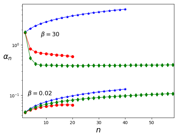
Refer to caption
Figure 15: Sequence of αnsubscript𝛼𝑛\alpha_{n} for the ideal gas limit (blue stars), for the nonlinear dynamics from the MD simulations (red dots) and for the harmonic regime (green diamonds).

We can see that for both the temperatures the sequence of the αnsubscript𝛼𝑛\alpha_{n} for the nonlinear and harmonic dynamics tends to a finite plateau; the ideal gas case shows instead a linear increase as expected. As discussed above, the finite asymptotic for the dynamic regimes is sufficient to predict a non-Gaussian relaxation.

A.9 Estimate of the high-order kernel coefficients

In this appendix we derive the estimate eqn. 24.
We can expand eqn. 19 as

κ2n2I=superscriptsubscript𝜅2𝑛2𝐼absent\displaystyle\kappa_{2n-2}^{I}= ω2nI+m=1n1χm(1)ω2(nm)Iω2mI+m=1n1m=1m1χm,m(2)ω2(nm)Iω2(mm)Iω2mI+subscriptsuperscript𝜔𝐼2𝑛superscriptsubscript𝑚1𝑛1subscriptsuperscript𝜒1𝑚subscriptsuperscript𝜔𝐼2𝑛𝑚subscriptsuperscript𝜔𝐼2𝑚superscriptsubscript𝑚1𝑛1superscriptsubscriptsuperscript𝑚1𝑚1subscriptsuperscript𝜒2𝑚superscript𝑚subscriptsuperscript𝜔𝐼2𝑛𝑚subscriptsuperscript𝜔𝐼2𝑚superscript𝑚subscriptsuperscript𝜔𝐼2superscript𝑚\displaystyle\omega^{I}_{2n}+\sum_{m=1}^{n-1}\chi^{(1)}_{m}\omega^{I}_{2(n-m)}\omega^{I}_{2m}+\sum_{m=1}^{n-1}\sum_{m^{\prime}=1}^{m-1}\chi^{(2)}_{m,m^{\prime}}\omega^{I}_{2(n-m)}\omega^{I}_{2(m-m^{\prime})}\omega^{I}_{2m^{\prime}}+\cdots
=\displaystyle= ω2nI(1+m=1n1χm(1)ω2(nm)Iω2mIω2nI+m=1n1m=1m1χm,m(2)ω2(nm)Iω2(mm)Iω2mIω2nI+)subscriptsuperscript𝜔𝐼2𝑛1superscriptsubscript𝑚1𝑛1subscriptsuperscript𝜒1𝑚subscriptsuperscript𝜔𝐼2𝑛𝑚subscriptsuperscript𝜔𝐼2𝑚subscriptsuperscript𝜔𝐼2𝑛superscriptsubscript𝑚1𝑛1superscriptsubscriptsuperscript𝑚1𝑚1subscriptsuperscript𝜒2𝑚superscript𝑚subscriptsuperscript𝜔𝐼2𝑛𝑚subscriptsuperscript𝜔𝐼2𝑚superscript𝑚subscriptsuperscript𝜔𝐼2superscript𝑚subscriptsuperscript𝜔𝐼2𝑛\displaystyle\omega^{I}_{2n}\left(1+\sum_{m=1}^{n-1}\chi^{(1)}_{m}\frac{\omega^{I}_{2(n-m)}\omega^{I}_{2m}}{\omega^{I}_{2n}}+\sum_{m=1}^{n-1}\sum_{m^{\prime}=1}^{m-1}\chi^{(2)}_{m,m^{\prime}}\frac{\omega^{I}_{2(n-m)}\omega^{I}_{2(m-m^{\prime})}\omega^{I}_{2m^{\prime}}}{\omega^{I}_{2n}}+\cdots\right) (56)

with suitable coefficients χm1,,mj(j)subscriptsuperscript𝜒𝑗subscript𝑚1subscript𝑚𝑗\chi^{(j)}_{m_{1},\cdots,m_{j}}. We can explicitly show that the non-constant contributions in eqn. 56 vanish via eqn. 23; starting from the first terms we get:

ω2(nm)Iω2mIω2nIsubscriptsuperscript𝜔𝐼2𝑛𝑚subscriptsuperscript𝜔𝐼2𝑚subscriptsuperscript𝜔𝐼2𝑛\displaystyle\frac{\omega^{I}_{2(n-m)}\omega^{I}_{2m}}{\omega^{I}_{2n}} =(1Cβ)(2(nm))!(nm)!(2m)!m!n!(2n)!2(1Cβ)(2(n1))!(n1)!n!(2n)!absent1subscript𝐶𝛽2𝑛𝑚𝑛𝑚2𝑚𝑚𝑛2𝑛21subscript𝐶𝛽2𝑛1𝑛1𝑛2𝑛\displaystyle=(1-C_{\beta})\frac{(2(n-m))!}{(n-m)!}\frac{(2m)!}{m!}\frac{n!}{(2n)!}\leq 2(1-C_{\beta})\frac{(2(n-1))!}{(n-1)!}\frac{n!}{(2n)!} (57)
2(1Cβ)n2n(2n1)n0absent21subscript𝐶𝛽𝑛2𝑛2𝑛1𝑛0\displaystyle\leq 2(1-C_{\beta})\frac{n}{2n(2n-1)}\xrightarrow{n\to\infty}0

where in the second line we noticed that m=1𝑚1m=1 corresponds to a maximum of the function

rn,m(2n2m)!(nm)!(2m)!m!subscript𝑟𝑛𝑚2𝑛2𝑚𝑛𝑚2𝑚𝑚\displaystyle r_{n,m}\equiv\frac{(2n-2m)!}{(n-m)!}\frac{(2m)!}{m!} (58)

This is shown by evaluating the increment

rn,m+1=subscript𝑟𝑛𝑚1absent\displaystyle r_{n,m+1}= (2n2m2)!(nm1)!(2m+2)!(m+1)!=(2n2m)!(2n2m)(2n2m1)nm(nm)!1m!(m+1)(2m)!(2m+1)(2m+2)=2𝑛2𝑚2𝑛𝑚12𝑚2𝑚12𝑛2𝑚2𝑛2𝑚2𝑛2𝑚1𝑛𝑚𝑛𝑚1𝑚𝑚12𝑚2𝑚12𝑚2absent\displaystyle\frac{(2n-2m-2)!}{(n-m-1)!}\frac{(2m+2)!}{(m+1)!}=\frac{(2n-2m)!}{(2n-2m)(2n-2m-1)}\frac{n-m}{(n-m)!}\frac{1}{m!(m+1)}(2m)!(2m+1)(2m+2)=
=\displaystyle= rn,mnm(2n2m)(2n2m1)(2m+1)(2m+2)(m+1)=rn,m2m+12n2m1=rn,mfn,msubscript𝑟𝑛𝑚𝑛𝑚2𝑛2𝑚2𝑛2𝑚12𝑚12𝑚2𝑚1subscript𝑟𝑛𝑚2𝑚12𝑛2𝑚1subscript𝑟𝑛𝑚subscript𝑓𝑛𝑚\displaystyle r_{n,m}\frac{n-m}{(2n-2m)(2n-2m-1)}\frac{(2m+1)(2m+2)}{(m+1)}=r_{n,m}\frac{2m+1}{2n-2m-1}=r_{n,m}f_{n,m}

where we defined

fn,m2m+12n2m1subscript𝑓𝑛𝑚2𝑚12𝑛2𝑚1f_{n,m}\equiv\frac{2m+1}{2n-2m-1} (59)

We can see that the discrete derivative of fn,msubscript𝑓𝑛𝑚f_{n,m} as a function of m𝑚m us always positive:

fn,m+1fn,m=4n(1+2m2n)(3+2m2n)4n(3+2m2n)20subscript𝑓𝑛𝑚1subscript𝑓𝑛𝑚4𝑛12𝑚2𝑛32𝑚2𝑛4𝑛superscript32𝑚2𝑛20\displaystyle f_{n,m+1}-f_{n,m}=\frac{4n}{(1+2m-2n)(3+2m-2n)}\geq\frac{4n}{(3+2m-2n)^{2}}\geq 0

The denominator of the last identity is always defined for m,n𝑚𝑛m,n\in\mathbb{N}. It then follows that fn,msubscript𝑓𝑛𝑚f_{n,m} is increasing with m𝑚m and

fn,m=1m=n12iffsubscript𝑓𝑛𝑚1𝑚𝑛12f_{n,m}=1\iff m=\frac{n-1}{2} (60)

Thus, rn,m+1rn,msubscript𝑟𝑛𝑚1subscript𝑟𝑛𝑚r_{n,m+1}\leq r_{n,m} if m(n1)/2𝑚𝑛12m\leq(n-1)/2 and vice-versa. Hence, the maximum values of rn,msubscript𝑟𝑛𝑚r_{n,m} are obtained at the boundaries of the admitted values of m𝑚m, i.e. m=1𝑚1m=1 and m=n1𝑚𝑛1m=n-1, as rn,1=rn,m1subscript𝑟𝑛1subscript𝑟𝑛𝑚1r_{n,1}=r_{n,m-1}.

A.10 Long-time decay of the memory kernel

In this section we estimate the long-time tail of KjI(t)superscriptsubscript𝐾𝑗𝐼𝑡K_{j}^{I}(t) in Fig. 11, in the high temperature regime. From Fig. 10 and Appendix A.9 we know that κ2nIω2n+2κ2n+2Isimilar-to-or-equalssuperscriptsubscript𝜅2𝑛𝐼subscript𝜔2𝑛2superscriptsubscript𝜅2𝑛2𝐼\kappa_{2n}^{I}\simeq\omega_{2n+2}\equiv\kappa_{2n+2}^{I} for n40greater-than-or-equivalent-to𝑛40n\gtrsim 40. We can extend this estimate for any value of n𝑛n and sum the resulting function, by assuming that for t1much-greater-than𝑡1t\gg 1 the higher series coefficients matter the most. The first issue that needs to be checked is whether the resulting series is convergent. From the ratio test we get:

limn+subscript𝑛\displaystyle\lim_{n\to+\infty} |t2n+2κ2n+2I(2n+2)!(2n)!t2nκ2nI|=t2limn+|an+2H2n+4(2n+2)!(2n)!an+1H2n+2|=at2limn+|(2)n+2(2n+3)!!(2n)!(2n+2)!(2)n+1(2n+1)!!|=superscript𝑡2𝑛2superscriptsubscript𝜅2𝑛2𝐼2𝑛22𝑛superscript𝑡2𝑛superscriptsubscript𝜅2𝑛𝐼superscript𝑡2subscript𝑛superscript𝑎𝑛2subscript𝐻2𝑛42𝑛22𝑛superscript𝑎𝑛1subscript𝐻2𝑛2𝑎superscript𝑡2subscript𝑛superscript2𝑛2double-factorial2𝑛32𝑛2𝑛2superscript2𝑛1double-factorial2𝑛1absent\displaystyle\left\lvert\frac{t^{2n+2}\kappa_{2n+2}^{I}}{(2n+2)!}\frac{(2n)!}{t^{2n}\kappa_{2n}^{I}}\right\rvert=t^{2}\lim_{n\to+\infty}\left\lvert\frac{a^{n+2}H_{2n+4}}{(2n+2)!}\frac{(2n)!}{a^{n+1}H_{2n+2}}\right\rvert=at^{2}\lim_{n\to+\infty}\left\lvert\frac{(-2)^{n+2}(2n+3)!!(2n)!}{(2n+2)!(-2)^{n+1}(2n+1)!!}\right\rvert=
=2at2limn+|(2(n+2))!2n+2(n+2)!(2n)!(2n+2)!(2(n+1))!2n+1(n+1)!|=2at2limn+(2n+4)(2n+3)2(2n+2)(2n+1)(n+2)=at2limn+1n=0absent2𝑎superscript𝑡2subscript𝑛2𝑛2superscript2𝑛2𝑛22𝑛2𝑛22𝑛1superscript2𝑛1𝑛12𝑎superscript𝑡2subscript𝑛2𝑛42𝑛322𝑛22𝑛1𝑛2𝑎superscript𝑡2subscript𝑛1𝑛0\displaystyle=2at^{2}\lim_{n\to+\infty}\left\lvert\frac{\frac{(2(n+2))!}{2^{n+2}(n+2)!}(2n)!}{(2n+2)!\frac{(2(n+1))!}{2^{n+1}(n+1)!}}\right\rvert=2at^{2}\lim_{n\to+\infty}\frac{(2n+4)(2n+3)}{2(2n+2)(2n+1)(n+2)}=at^{2}\lim_{n\to+\infty}\frac{1}{n}=0

This shows that the radius of convergence of the series obtained with the approximation κ2nκ2nIsimilar-to-or-equalssubscript𝜅2𝑛superscriptsubscript𝜅2𝑛𝐼\kappa_{2n}\simeq\kappa_{2n}^{I} is infinite; we can therefore sum the approximation of the tail for any value of n𝑛n:

Kj(t)t1n=0+t2n(2n)!ω2n+2I=n=0+t2n(2n)![(1Cβ)an+1H2n+2+δn+1,0Cβ]=subscriptsimilar-to-or-equalsmuch-greater-than𝑡1subscript𝐾𝑗𝑡superscriptsubscript𝑛0superscript𝑡2𝑛2𝑛subscriptsuperscript𝜔𝐼2𝑛2superscriptsubscript𝑛0superscript𝑡2𝑛2𝑛delimited-[]1subscript𝐶𝛽superscript𝑎𝑛1subscript𝐻2𝑛2subscript𝛿𝑛10subscript𝐶𝛽absent\displaystyle K_{j}(t)\simeq_{t\gg 1}\sum_{n=0}^{+\infty}\frac{t^{2n}}{(2n)!}\omega^{I}_{2n+2}=\sum_{n=0}^{+\infty}\frac{t^{2n}}{(2n)!}\left[(1-C_{\beta})a^{n+1}H_{2n+2}+\delta_{n+1,0}C_{\beta}\right]=
=n=0+t2n(2n)![(1Cβ)an+1(2)n+1(2n+1)!!]=(1Cβ)n=0+t2n(2n)!an+1(2)n+12n+1Γ(n+32)π=absentsuperscriptsubscript𝑛0superscript𝑡2𝑛2𝑛delimited-[]1subscript𝐶𝛽superscript𝑎𝑛1superscript2𝑛1double-factorial2𝑛11subscript𝐶𝛽superscriptsubscript𝑛0superscript𝑡2𝑛2𝑛superscript𝑎𝑛1superscript2𝑛1superscript2𝑛1Γ𝑛32𝜋absent\displaystyle=\sum_{n=0}^{+\infty}\frac{t^{2n}}{(2n)!}\left[(1-C_{\beta})a^{n+1}(-2)^{n+1}(2n+1)!!\right]=(1-C_{\beta})\sum_{n=0}^{+\infty}\frac{t^{2n}}{(2n)!}a^{n+1}(-2)^{n+1}\frac{2^{n+1}\Gamma(n+\frac{3}{2})}{\sqrt{\pi}}=
=(1Cβ)n=0+(1)n+1t2n(2n)!an+14n+1ππ(2n+2)!4n+1(n+1)!=(1Cβ)an=0+(1)n+1(at2)n(2n+2)(2n+1)(n+1)!=absent1subscript𝐶𝛽superscriptsubscript𝑛0superscript1𝑛1superscript𝑡2𝑛2𝑛superscript𝑎𝑛1superscript4𝑛1𝜋𝜋2𝑛2superscript4𝑛1𝑛11subscript𝐶𝛽𝑎superscriptsubscript𝑛0superscript1𝑛1superscript𝑎superscript𝑡2𝑛2𝑛22𝑛1𝑛1absent\displaystyle=(1-C_{\beta})\sum_{n=0}^{+\infty}(-1)^{n+1}\frac{t^{2n}}{(2n)!}a^{n+1}\frac{4^{n+1}}{\sqrt{\pi}}\frac{\sqrt{\pi}(2n+2)!}{4^{n+1}(n+1)!}=(1-C_{\beta})a\sum_{n=0}^{+\infty}(-1)^{n+1}\left(at^{2}\right)^{n}\frac{(2n+2)(2n+1)}{(n+1)!}=
=(1Cβ)an=0+(1)n+1(at2)n(2n+2)(2n+1)(n+1)!=2(1Cβ)aeat2(2at21)absent1subscript𝐶𝛽𝑎superscriptsubscript𝑛0superscript1𝑛1superscript𝑎superscript𝑡2𝑛2𝑛22𝑛1𝑛121subscript𝐶𝛽𝑎superscript𝑒𝑎superscript𝑡22𝑎superscript𝑡21\displaystyle=(1-C_{\beta})a\sum_{n=0}^{+\infty}(-1)^{n+1}\left(at^{2}\right)^{n}\frac{(2n+2)(2n+1)}{(n+1)!}=2(1-C_{\beta})ae^{-at^{2}}(2at^{2}-1) (61)

which means

Kj(t)Kj(0)t1eat2(12at2)subscriptsimilar-to-or-equalsmuch-greater-than𝑡1subscript𝐾𝑗𝑡subscript𝐾𝑗0superscript𝑒𝑎superscript𝑡212𝑎superscript𝑡2\frac{K_{j}(t)}{K_{j}(0)}\simeq_{t\gg 1}e^{-at^{2}}(1-2at^{2}) (62)

From the result above we can choose the following ansatz for the long time limit:

Kj(t)t1At2eBt2subscriptsimilar-to-or-equalsmuch-greater-than𝑡1subscript𝐾𝑗𝑡𝐴superscript𝑡2superscript𝑒𝐵superscript𝑡2K_{j}(t)\simeq_{t\gg 1}At^{2}e^{-Bt^{2}}

The coefficients A𝐴A and B𝐵B can be fixed for each temperature by extending the sum in eqn. 25 continuously with continuous derivative from a time t=t(β)superscript𝑡superscript𝑡𝛽t^{*}=t^{*}(\beta) before its divergence The parameters A𝐴A and B𝐵B are then fixed by

A𝐴\displaystyle A =Kt2exp(Kt2K2K)absentsuperscript𝐾superscriptsuperscript𝑡2superscriptsuperscript𝐾superscript𝑡2superscript𝐾2superscript𝐾\displaystyle=\frac{K^{*}}{{t^{*}}^{2}\exp\left(\frac{{K^{\prime}}^{*}t^{*}-2K^{*}}{2K^{*}}\right)}
B𝐵\displaystyle B =2KKt2Kt2absent2superscript𝐾superscriptsuperscript𝐾superscript𝑡2superscript𝐾superscriptsuperscript𝑡2\displaystyle=\frac{2K^{*}-{K^{\prime}}^{*}t^{*}}{2K^{*}{t^{*}}^{2}}

where

Ksuperscript𝐾\displaystyle K^{*} KNmax(t)absentsubscript𝐾subscript𝑁𝑚𝑎𝑥superscript𝑡\displaystyle\equiv K_{N_{max}}(t^{*})
Ksuperscriptsuperscript𝐾\displaystyle{K^{\prime}}^{*} n=0Nmaxκ2n(2n1)!t2n1absentsuperscriptsubscript𝑛0subscript𝑁𝑚𝑎𝑥subscript𝜅2𝑛2𝑛1superscriptsuperscript𝑡2𝑛1\displaystyle\equiv\sum_{n=0}^{N_{max}}\frac{\kappa_{2n}}{(2n-1)!}{t^{*}}^{2n-1}

We can additionally check that the series obtained by summing the first neglected terms in the expansion of the kernel eqn. 56 is convergent. Although this is far from proving the boundedness of the infinitely many orders neglected, it represents a necessary condition. The time-series of the first order correction is given by

K1I(t)n=0+t2n(2n)!m=1nχm(1)ω2(nm+1)Iω2mI=n=0+t2n(2n)!m=1nχm(1)[(1Cβ)anm+1H2(nm+1)][(1Cβ)amH2m]=superscriptsubscript𝐾1𝐼𝑡superscriptsubscript𝑛0superscript𝑡2𝑛2𝑛superscriptsubscript𝑚1𝑛superscriptsubscript𝜒𝑚1superscriptsubscript𝜔2𝑛𝑚1𝐼superscriptsubscript𝜔2𝑚𝐼superscriptsubscript𝑛0superscript𝑡2𝑛2𝑛superscriptsubscript𝑚1𝑛superscriptsubscript𝜒𝑚1delimited-[]1subscript𝐶𝛽superscript𝑎𝑛𝑚1subscript𝐻2𝑛𝑚1delimited-[]1subscript𝐶𝛽superscript𝑎𝑚subscript𝐻2𝑚absent\displaystyle K_{1}^{I}(t)\equiv\sum_{n=0}^{+\infty}\frac{t^{2n}}{(2n)!}\sum_{m=1}^{n}\chi_{m}^{(1)}\omega_{2(n-m+1)}^{I}\omega_{2m}^{I}=\sum_{n=0}^{+\infty}\frac{t^{2n}}{(2n)!}\sum_{m=1}^{n}\chi_{m}^{(1)}\left[(1-C_{\beta})a^{n-m+1}H_{2(n-m+1)}\right]\left[(1-C_{\beta})a^{m}H_{2m}\right]=
=(1Cβ)2n=0+an+1t2n(2n)!m=1n(2)nm+1(2(nm)+1)!!(2)m(2m1)!!=absentsuperscript1subscript𝐶𝛽2superscriptsubscript𝑛0superscript𝑎𝑛1superscript𝑡2𝑛2𝑛superscriptsubscript𝑚1𝑛superscript2𝑛𝑚1double-factorial2𝑛𝑚1superscript2𝑚double-factorial2𝑚1absent\displaystyle=-(1-C_{\beta})^{2}\sum_{n=0}^{+\infty}a^{n+1}\frac{t^{2n}}{(2n)!}\sum_{m=1}^{n}(-2)^{n-m+1}\left(2(n-m)+1\right)!!(-2)^{m}(2m-1)!!=
=(1Cβ)2n=0+(2a)n+1t2n(2n)!m=1n(2(nm+1))!2nm+1(nm+1)!(2m)!2mm!=absentsuperscript1subscript𝐶𝛽2superscriptsubscript𝑛0superscript2𝑎𝑛1superscript𝑡2𝑛2𝑛superscriptsubscript𝑚1𝑛2𝑛𝑚1superscript2𝑛𝑚1𝑛𝑚12𝑚superscript2𝑚𝑚absent\displaystyle=-(1-C_{\beta})^{2}\sum_{n=0}^{+\infty}(-2a)^{n+1}\frac{t^{2n}}{(2n)!}\sum_{m=1}^{n}\frac{\left(2(n-m+1)\right)!}{2^{n-m+1}(n-m+1)!}\frac{(2m)!}{2^{m}m!}=
=(1Cβ)2an=0+(at2)n(2n)!m=1n(2(nm+1))!(nm+1)!(2m)!m!n=0+anabsentsuperscript1subscript𝐶𝛽2𝑎superscriptsubscript𝑛0superscript𝑎superscript𝑡2𝑛2𝑛superscriptsubscript𝑚1𝑛2𝑛𝑚1𝑛𝑚12𝑚𝑚superscriptsubscript𝑛0subscript𝑎𝑛\displaystyle=-(1-C_{\beta})^{2}a\sum_{n=0}^{+\infty}\frac{\left(-at^{2}\right)^{n}}{(2n)!}\sum_{m=1}^{n}\frac{\left(2(n-m+1)\right)!}{(n-m+1)!}\frac{(2m)!}{m!}\equiv\sum_{n=0}^{+\infty}a_{n} (63)

where in the second line we used the property χm(1)=1msubscriptsuperscript𝜒1𝑚1for-all𝑚\chi^{(1)}_{m}=-1\;\;\forall m, as it can be explicitly checked from the recursive reconstruction of the relation eqn. 19 till high orders. Following the same argument presented in Appendix A.9, we can determine

maxm{1,n}(2(nm+1))!(nm+1)!(2m)!m!=(2(nm+1))!(nm+1)!(2m)!m!|m=1m=n=2(2n)!n!subscript𝑚1𝑛2𝑛𝑚1𝑛𝑚12𝑚𝑚evaluated-at2𝑛𝑚1𝑛𝑚12𝑚𝑚𝑚1𝑚𝑛22𝑛𝑛\max_{m\in\left\{1,n\right\}}\frac{\left(2(n-m+1)\right)!}{(n-m+1)!}\frac{(2m)!}{m!}=\left.\frac{\left(2(n-m+1)\right)!}{(n-m+1)!}\frac{(2m)!}{m!}\right|_{\begin{subarray}{c}m=1\\ m=n\end{subarray}}=2\frac{(2n)!}{n!}

We can then check the convergence of the series in eqn. 63 via the direct comparison test:

|an||(1Cβ)22a(at2)n(2n)!n(2n)!n!||bn|=|(1Cβ)22a(at2)n(n1)!||bn1|,n1formulae-sequencesubscript𝑎𝑛superscript1subscript𝐶𝛽22𝑎superscript𝑎superscript𝑡2𝑛2𝑛𝑛2𝑛𝑛subscript𝑏𝑛superscript1subscript𝐶𝛽22𝑎superscript𝑎superscript𝑡2𝑛𝑛1subscript𝑏𝑛1𝑛1\displaystyle\left\lvert a_{n}\right\rvert\leq\left\lvert-(1-C_{\beta})^{2}2a\frac{(-at^{2})^{n}}{(2n)!}n\frac{(2n)!}{n!}\right\rvert\equiv\left\lvert b_{n}\right\rvert=\left\lvert-(1-C_{\beta})^{2}2a\frac{(-at^{2})^{n}}{(n-1)!}\right\rvert\equiv\left\lvert b_{n-1}\right\rvert,\hskip 14.22636ptn\geq 1

Via the ratio test we can notice that the series n=0+bnsuperscriptsubscript𝑛0subscript𝑏𝑛\sum_{n=0}^{+\infty}b_{n} is convergent:

limn+|bn+1bn|=limn+|at2|(n1)!n!=|at2|limn+1n=0subscript𝑛subscript𝑏𝑛1subscript𝑏𝑛subscript𝑛𝑎superscript𝑡2𝑛1𝑛𝑎superscript𝑡2subscript𝑛1𝑛0\displaystyle\lim_{n\to+\infty}\left\lvert\frac{b_{n+1}}{b_{n}}\right\rvert=\lim_{n\to+\infty}\left\lvert-at^{2}\right\rvert\frac{(n-1)!}{n!}=\left\lvert-at^{2}\right\rvert\lim_{n\to+\infty}\frac{1}{n}=0

which then proves the convergence of eqn. 63.

A.11 Management of high-dimensional tensors

The components of 𝐦𝐬(n)superscriptsubscript𝐦𝐬𝑛\mathcal{I}_{\mathbf{ms}}^{(n)} can be stored in a one-dimensional pointer in row-major order. For example the indeces of a 3×3×33333\times 3\times 3 tensor would be sorted as

{000,001,002,010,011,012,021,,222}000001002010011012021222\left\{000,001,002,010,011,012,021,\cdots,222\right\}

and by mapping the sequence of the indexes into integer numbers according to

(i,j,k)i102+j10+k𝑖𝑗𝑘𝑖superscript102𝑗10𝑘(i,j,k)\rightarrow i\cdot 10^{2}+j\cdot 10+k

we get a monotonically increasing sequence. In this case, let us define a general label

𝐯={v0,,vnind1}𝐯subscript𝑣0subscript𝑣subscriptnind1\mathbf{v}=\{v_{0},\cdots,v_{\operatorname{n_{\operatorname{ind}}}-1}\}

of a tensor 𝒜𝒜\mathcal{A} of dimension 𝐃={D0,,Dnind1}nind𝐃subscript𝐷0subscript𝐷subscriptnind1superscriptsubscript𝑛𝑖𝑛𝑑\mathbf{D}=\left\{D_{0},\cdots,D_{\operatorname{n_{\operatorname{ind}}}-1}\right\}\in\mathbb{N}^{n_{ind}} and complex images; Djcar({vj})subscript𝐷𝑗carsubscript𝑣𝑗D_{j}\equiv\operatorname{car}\left(\left\{v_{j}\right\}\right) is the cardinality of the set of the allowed values of the vjsubscript𝑣𝑗v_{j}. In our case vj{0}subscript𝑣𝑗0v_{j}\in\mathbb{N}\cup\{0\} is a power of a certain coordinate of the system; it follows that vj{0,1,,Dj1}subscript𝑣𝑗01subscript𝐷𝑗1v_{j}\in\{0,1,\cdots,D_{j}-1\}. Any entry of the tensor 𝒜𝐯subscript𝒜𝐯\mathcal{A}_{\mathbf{v}}\in\mathbb{C} can be mapped as an entry of a one dimensional array via the function

map(𝐯,𝐃,nind)=v0β0=1nind1Dβ0+v1β1=2nind1Dβ1+vnind1=α=0nind1vαβα=α+1nind1Dβαmap𝐯𝐃subscriptnindsubscript𝑣0superscriptsubscriptproductsubscript𝛽01subscriptnind1subscript𝐷subscript𝛽0subscript𝑣1superscriptsubscriptproductsubscript𝛽12subscript𝑛𝑖𝑛𝑑1subscript𝐷subscript𝛽1subscript𝑣subscriptnind1superscriptsubscript𝛼0subscript𝑛𝑖𝑛𝑑1subscript𝑣𝛼superscriptsubscriptproductsubscript𝛽𝛼𝛼1subscript𝑛𝑖𝑛𝑑1subscript𝐷subscript𝛽𝛼\operatorname{map}(\mathbf{v},\mathbf{D},\operatorname{n_{\operatorname{ind}}})=v_{0}\prod_{\beta_{0}=1}^{\operatorname{n_{\operatorname{ind}}}-1}D_{\beta_{0}}+v_{1}\prod_{\beta_{1}=2}^{n_{ind}-1}D_{\beta_{1}}+\cdots v_{\operatorname{n_{\operatorname{ind}}}-1}=\sum_{\alpha=0}^{n_{ind}-1}v_{\alpha}\prod_{\beta_{\alpha}=\alpha+1}^{n_{ind}-1}D_{\beta_{\alpha}} (64)

It is straightforward to determine the map of last index of the tensor 𝐯last{D01,D11,,Dnind11}subscript𝐯𝑙𝑎𝑠𝑡subscript𝐷01subscript𝐷11subscript𝐷subscriptnind11\mathbf{v}_{last}\equiv\{D_{0}-1,D_{1}-1,\cdots,D_{\operatorname{n_{\operatorname{ind}}}-1}-1\}:

map(𝐯last,𝐃,nind)mapsubscript𝐯𝑙𝑎𝑠𝑡𝐃subscriptnind\displaystyle\operatorname{map}(\mathbf{v}_{last},\mathbf{D},\operatorname{n_{\operatorname{ind}}}) =α=0nind1(Dα1)βα=α+1nind1Dβα=[(D01)D1D2Dnind1]+absentsuperscriptsubscript𝛼0subscriptnind1subscript𝐷𝛼1superscriptsubscriptproductsubscript𝛽𝛼𝛼1subscript𝑛𝑖𝑛𝑑1subscript𝐷subscript𝛽𝛼limit-fromdelimited-[]subscript𝐷01subscript𝐷1subscript𝐷2subscript𝐷subscriptnind1\displaystyle=\sum_{\alpha=0}^{\operatorname{n_{\operatorname{ind}}}-1}(D_{\alpha}-1)\prod_{\beta_{\alpha}=\alpha+1}^{n_{ind}-1}D_{\beta_{\alpha}}=\left[(D_{0}-1)D_{1}D_{2}\cdots D_{\operatorname{n_{\operatorname{ind}}}-1}\right]+
+[(D11)D2Dnind1]++Dnind11=γ=0nind1Dγ1M𝐃delimited-[]subscript𝐷11subscript𝐷2subscript𝐷subscriptnind1subscript𝐷subscriptnind11superscriptsubscriptproduct𝛾0subscriptnind1subscript𝐷𝛾1subscript𝑀𝐃\displaystyle+\left[(D_{1}-1)D_{2}\cdots D_{\operatorname{n_{\operatorname{ind}}}-1}\right]+\cdots+D_{\operatorname{n_{\operatorname{ind}}}-1}-1=\prod_{\gamma=0}^{\operatorname{n_{\operatorname{ind}}}-1}D_{\gamma}-1\equiv M_{\mathbf{D}}

The identity follows as the sum is telescopic.

In the implementation of the recursion relations in Section 4 controlling (i)neiKrj(i)n+1eiKrjsuperscript𝑖𝑛superscript𝑒𝑖𝐾subscript𝑟𝑗superscript𝑖𝑛1superscript𝑒𝑖𝐾subscript𝑟𝑗(i\mathcal{L})^{n}e^{iKr_{j}}\rightarrow(i\mathcal{L})^{n+1}e^{iKr_{j}} we are interested in integer increments (let us say by l𝑙l\in\mathbb{N}) of a generic i𝑖i-th ’column’ of the coefficients tensor: 𝐦𝐬(n)I𝐦𝐬+l𝐞^𝐢(n)subscriptsuperscript𝑛𝐦𝐬subscriptsuperscript𝐼𝑛𝐦𝐬𝑙subscript^𝐞𝐢\mathcal{I}^{(n)}_{\mathbf{ms}}\rightarrow I^{(n)}_{\mathbf{ms}+l\mathbf{\hat{e}_{i}}}. By imposing vil{0,,Di1}subscript𝑣𝑖𝑙0subscript𝐷𝑖1v_{i}\equiv l\in\{0,\cdots,D_{i}-1\}, it directly follows from eqn. 64:

map({v0,,vi1,l,vi+1,,vnind1},𝐃,nind)=α=0αinind1vαβα=α+1nind1Dβα+lβi=i+1nind1Dβimapsubscript𝑣0subscript𝑣𝑖1𝑙subscript𝑣𝑖1subscript𝑣subscriptnind1𝐃subscriptnindsuperscriptsubscript𝛼0𝛼𝑖subscriptnind1subscript𝑣𝛼superscriptsubscriptproductsubscript𝛽𝛼𝛼1subscript𝑛𝑖𝑛𝑑1subscript𝐷subscript𝛽𝛼𝑙superscriptsubscriptproductsubscript𝛽𝑖𝑖1subscript𝑛𝑖𝑛𝑑1subscript𝐷subscript𝛽𝑖\displaystyle\operatorname{map}(\{v_{0},\cdots,v_{i-1},l,v_{i+1},\cdots,v_{\operatorname{n_{\operatorname{ind}}}-1}\},\mathbf{D},\operatorname{n_{\operatorname{ind}}})=\sum_{\begin{subarray}{c}\alpha=0\\ \alpha\neq i\end{subarray}}^{\operatorname{n_{\operatorname{ind}}}-1}v_{\alpha}\prod_{\beta_{\alpha}=\alpha+1}^{n_{ind}-1}D_{\beta_{\alpha}}+l\prod_{\beta_{i}=i+1}^{n_{ind}-1}D_{\beta_{i}}

It is moreover possible to determine the inverse map that, given an entry of a one-dimensional mapping and the list of the related dimensions, returns the multi-index associated to that component. For this we can proceed recursively, from the extraction of the last index vnind1subscript𝑣subscriptnind1v_{\operatorname{n_{\operatorname{ind}}}-1} backwards. From eqn. 64 we get:

nmapmap(𝐯,𝐃,nind)subscriptnmapmap𝐯𝐃subscriptnind\displaystyle\operatorname{n_{\operatorname{map}}}\equiv\operatorname{map}(\mathbf{v},\mathbf{D},\operatorname{n_{\operatorname{ind}}}) =(α=0nind2vαβα=α+1nind1Dβα)+vnind1=(α=0nind2vαβα=α+1nind2Dβα)Dnind1+vnind1absentsuperscriptsubscript𝛼0subscriptnind2subscript𝑣𝛼superscriptsubscriptproductsubscript𝛽𝛼𝛼1subscriptnind1subscript𝐷subscript𝛽𝛼subscript𝑣subscriptnind1superscriptsubscript𝛼0subscriptnind2subscript𝑣𝛼superscriptsubscriptproductsubscript𝛽𝛼𝛼1subscriptnind2subscript𝐷subscript𝛽𝛼subscript𝐷subscriptnind1subscript𝑣subscriptnind1\displaystyle=\left(\sum_{\alpha=0}^{\operatorname{n_{\operatorname{ind}}}-2}v_{\alpha}\prod_{\beta_{\alpha}=\alpha+1}^{\operatorname{n_{\operatorname{ind}}}-1}D_{\beta_{\alpha}}\right)+v_{\operatorname{n_{\operatorname{ind}}}-1}=\left(\sum_{\alpha=0}^{\operatorname{n_{\operatorname{ind}}}-2}v_{\alpha}\prod_{\beta_{\alpha}=\alpha+1}^{\operatorname{n_{\operatorname{ind}}}-2}D_{\beta_{\alpha}}\right)D_{\operatorname{n_{\operatorname{ind}}}-1}+v_{\operatorname{n_{\operatorname{ind}}}-1} (65)
vnind1subscript𝑣subscriptnind1\displaystyle v_{\operatorname{n_{\operatorname{ind}}}-1} =nmapmodDnind1absentmodulosubscriptnmapsubscript𝐷subscriptnind1\displaystyle=\operatorname{n_{\operatorname{map}}}\mod D_{\operatorname{n_{\operatorname{ind}}}-1} (66)

Eqn. 66 follows from eqn. 65 being vnind1<Dnind1subscript𝑣subscriptnind1subscript𝐷subscriptnind1v_{\operatorname{n_{\operatorname{ind}}}-1}<D_{\operatorname{n_{\operatorname{ind}}}-1}. We can proceed with the extraction of the second last component vnind2subscript𝑣subscriptnind2v_{\operatorname{n_{\operatorname{ind}}}-2} via the knowledge of vnind1subscript𝑣subscriptnind1v_{\operatorname{n_{\operatorname{ind}}}-1}:

Anind1nmapvnind1Dnind1subscript𝐴subscript𝑛𝑖𝑛𝑑1subscriptnmapsubscript𝑣subscriptnind1subscript𝐷subscriptnind1\displaystyle A_{n_{ind}-1}\equiv\frac{\operatorname{n_{\operatorname{map}}}-v_{\operatorname{n_{\operatorname{ind}}}-1}}{D_{\operatorname{n_{\operatorname{ind}}}-1}} =(α=0nind3vαβα=α+1nind3Dβα)Dnind2+vnind2absentsuperscriptsubscript𝛼0subscriptnind3subscript𝑣𝛼superscriptsubscriptproductsubscript𝛽𝛼𝛼1subscriptnind3subscript𝐷subscript𝛽𝛼subscript𝐷subscriptnind2subscript𝑣subscriptnind2\displaystyle=\left(\sum_{\alpha=0}^{\operatorname{n_{\operatorname{ind}}}-3}v_{\alpha}\prod_{\beta_{\alpha}=\alpha+1}^{\operatorname{n_{\operatorname{ind}}}-3}D_{\beta_{\alpha}}\right)D_{\operatorname{n_{\operatorname{ind}}}-2}+v_{\operatorname{n_{\operatorname{ind}}}-2}
vnind2subscript𝑣subscriptnind2\displaystyle v_{\operatorname{n_{\operatorname{ind}}}-2} =Anind1modDnind2absentmodulosubscript𝐴subscript𝑛𝑖𝑛𝑑1subscript𝐷subscriptnind2\displaystyle=A_{n_{ind}-1}\mod D_{\operatorname{n_{\operatorname{ind}}}-2}

A recursion relation can then be established i{0,,nind1}for-all𝑖0subscriptnind1\forall\;\;i\in\{0,\cdots,\operatorname{n_{\operatorname{ind}}}-1\}:

vnindi1subscript𝑣subscriptnind𝑖1\displaystyle v_{\operatorname{n_{\operatorname{ind}}}-i-1} =AnindimodDnindi1absentmodulosubscript𝐴subscriptnind𝑖subscript𝐷subscriptnind𝑖1\displaystyle=A_{\operatorname{n_{\operatorname{ind}}}-i}\mod D_{\operatorname{n_{\operatorname{ind}}}-i-1}
Anindi1subscript𝐴subscriptnind𝑖1\displaystyle A_{\operatorname{n_{\operatorname{ind}}}-i-1} =Anindivnindi1Dnindi1absentsubscript𝐴subscriptnind𝑖subscript𝑣subscriptnind𝑖1subscript𝐷subscriptnind𝑖1\displaystyle=\frac{A_{\operatorname{n_{\operatorname{ind}}}-i}-v_{\operatorname{n_{\operatorname{ind}}}-i-1}}{D_{\operatorname{n_{\operatorname{ind}}}-i-1}}

with initial condition Anind=nmapsubscript𝐴subscriptnindsubscriptnmapA_{\operatorname{n_{\operatorname{ind}}}}=\operatorname{n_{\operatorname{map}}}.


Acknowledgments

We thank T. Voigtmann, T. Franosch and A. Zippelius for useful discussions. Computer simulations presented in this paper were carried out using the bwForCluster NEMO high-performance computing facility.

References

  • [1] M. Peyrard and J. Farago, “Nonlinear localization in thermalized lattices: application to DNA,” Physica A: Statistical Mechanics and its Applications, vol. 288, no. 1, pp. 199 – 217, 2000.
  • [2] A. Henry and G. Chen, “Anomalous heat conduction in polyethylene chains: Theory and molecular dynamics simulations,” Phys. Rev. B, vol. 79, p. 144305, Apr 2009.
  • [3] H. Spohn, “Exact solutions for KPZ-type growth processes, random matrices, and equilibrium shapes of crystals,” Physica A: Statistical Mechanics and its Applications, vol. 369, no. 1, pp. 71 – 99, 2006.
  • [4] G. Gallavotti, The Fermi-Pasta-Ulam Problem: A Status Report. Berlin, Heidelberg: Springer, 2008.
  • [5] D. Bambusi, A. Carati, A. Maiocchi, and A. Maspero, Some Analytic Results on the FPU Paradox, pp. 235–254. New York, NY: Springer New York, 2015.
  • [6] E. Fermi, J. Pasta, and S. Ulam, “Studies of nonlinear problems I, Los Alamos Report LA 1940, 1955,” 1974.
  • [7] T. Dauxois, “Fermi, Pasta, Ulam, and a mysterious lady,” Physics Today, vol. 61, no. 1, pp. 55–57, 2008.
  • [8] E. Fermi, “Beweiss das ein mechanisches Normalsystem im allgemeinen quasi-ergodisch ist,” Phys. Z., vol. 24, p. 261, 1923.
  • [9] B. Rink, “Proof of Nishida’s Conjecture on Anharmonic Lattices,” Communications in Mathematical Physics, vol. 261, no. 3, pp. 613–627, 2006.
  • [10] G. Friesecke and A. Mikikits-Leitner, “Cnoidal Waves on Fermi–Pasta–Ulam Lattices,” vol. 27, 01 2014.
  • [11] D. Hajnal and R. Schilling, “Delocalization-localization transition due to anharmonicity,” Phys. Rev. Lett., vol. 101, p. 124101, Sep 2008.
  • [12] A. Carati and L. Galgani, “Metastability in specific-heat measurements: Simulations with the FPU model,” EPL (Europhysics Letters), vol. 75, no. 4, p. 528, 2006.
  • [13] A. Maiocchi, D. Bambusi, and A. Carati, “An averaging theorem for fpu in the thermodynamic limit,” Journal of Statistical Physics, vol. 155, pp. 300–322, Apr 2014.
  • [14] A. M. Maiocchi, A. Carati, and A. Giorgilli, “A series expansion for the time autocorrelation of dynamical variables,” Journal of Statistical Physics, vol. 148, pp. 1054–1071, Sep 2012.
  • [15] A. Carati, A. Maiocchi, L. Galgani, and G. Amati, “The Fermi–Pasta–Ulam System as a Model for Glasses,” Mathematical Physics, Analysis and Geometry, vol. 18, p. 31, Nov 2015.
  • [16] H. Mori, “Transport, Collective Motion, and Brownian Motion,” Progress of Theoretical Physics, vol. 33, no. 3, pp. 423–455, 1965.
  • [17] R. Zwanzig, “Memory Effects in Irreversible Thermodynamics,” Phys. Rev., vol. 124, pp. 983–992, Nov 1961.
  • [18] H. Grabert, Projection operator techniques in nonequilibrium statistical mechanics. Berlin: Springer, 1982.
  • [19] A. Wierling, “Dynamic structure factor of linear harmonic chain – a recurrence relation approach,” The European Physical Journal B, vol. 85, Jan 2012.
  • [20] H. Meyer, T. Voigtmann, and T. Schilling, “On the non-stationary generalized Langevin equation,” The Journal of chemical physics, vol. 147, p. 214110, Aug 2017.
  • [21] M. P. Allen and D. J. Tildesley, Computer Simulation of Liquids. New York, NY, USA: Clarendon Press, 1989.
  • [22] D. R. Reichman and P. Charbonneau, “Mode-coupling theory,” Journal of Statistical Mechanics: Theory and Experiment, vol. 2005, no. 05, p. P05013, 2005.
  • [23] J.-P. Hansen and I. R. McDonald, eds., Theory of Simple Liquids (Fourth Edition). Oxford: Academic Press, 2013.
  • [24] B. Jean‐Philippe, Anomalous Relaxation in Complex Systems: From Stretched to Compressed Exponentials, ch. 11, pp. 327–345. Wiley-Blackwell, 2008.
  • [25] T. Yoshida, K. Shobu, and H. Mori, “Dynamic properties of one-dimensional harmonic liquids. idensity correlation and transport coefficients,” Progress of Theoretical Physics, vol. 66, no. 3, pp. 759–771, 1981.
  • [26] K. Shobu, T. Yoshida, and H. Mori, “Dynamic properties of one-dimensional harmonic liquids. ii— energy density correlation and heat transport,” Progress of Theoretical Physics, vol. 66, no. 4, pp. 1160–1168, 1981.
  • [27] G. Radons, J. Keller, and T. Geisel, “Dynamical structure factor of a one-dimensional harmonic liquid: Comparison of different approximation methods,” Zeitschrift für Physik B Condensed Matter, vol. 50, pp. 289–296, Dec 1983.