Tight Bound of Incremental Cover Trees
for Dynamic Diversification

Abstract

Dynamic diversification—finding a set of data points with maximum diversity from a time-dependent sample pool—is an important task in recommender systems, web search, database search, and notification services, to avoid showing users duplicate or very similar items. The incremental cover tree (ICT) with high computational efficiency and flexibility has been applied to this task, and shown good performance. Specifically, it was empirically observed that ICT typically provides a set with its diversity only marginally ($\sim 1/1.2$ times) worse than the greedy max-min (GMM) algorithm, the state-of-the-art method for static diversification with its performance bound optimal for any polynomial time algorithm. Nevertheless, the known performance bound for ICT is 4 times worse than this optimal bound. With this paper, we aim to fill this very gap between theory and empirical observations. For achieving this, we first analyze variants of ICT methods, and derive tighter performance bounds. We then investigate the gap between the obtained bound and empirical observations by using specially designed artificial data for which the optimal diversity is known. Finally, we analyze the tightness of the bound, and show that the bound cannot be further improved, i.e., this paper provides the tightest possible bound for ICT methods. In addition, we demonstrate a new use of dynamic diversification for generative image samplers, where prototypes are incrementally collected from a stream of artificial images generated by an image sampler.

1 Introduction

The diversification problem is a notoriously important issue in a number of popular applications, e.g., in recommender systems [24, 23, 22], web search [11, 20], and database search [19, 6, 15]. Diversity helps to avoid showing users duplicate or very similar items, etc. Formally, it is defined as follows:

Definition 1

(Diversification problem) Let $V=\{v_{1},\ldots v_{N}\}$ be a set of $N$ points in some metric space $(\mathcal{V},d)$ with distance metric $d:\mathcal{V}\times\mathcal{V}\rightarrow\mathbb{R}^{+}$. The goal of the $k$-max-min diversification problem (for $k\leq N$) is to select a subset $S$ of $V$ such that

$$\textstyle S=\mathop{\mathrm{argmax}}_{S^{\prime}\subseteq V,|S^{\prime}|=k}\;\;div(S^{\prime}),$$ (1)

where the diversity is defined as the minimum distance of any pair of data points in a set, i.e.,

$$\textstyle div(S^{\prime})=\min_{s,s^{\prime}\in S^{\prime},s\neq s^{\prime}}\;\;d(s,s^{\prime}).$$ (2)

This problem is known to be NP-hard [9], and variety of approximation methods have been proposed [9, 18, 10, 20, 16, 8]. Among them, greedy max-min [18] is one of the state-of-the-art methods, although it was proposed several decades ago [10, 8]. It was shown that GMM is guaranteed to provide an approximate solution with its diversity no smaller than $d^{*}/2$, where $d^{*}$ is the diversity of the optimal solution [18]. Furthermore, it was also shown that $d^{*}/2$ is the best achievable bound by any polynomial time algorithm [18].

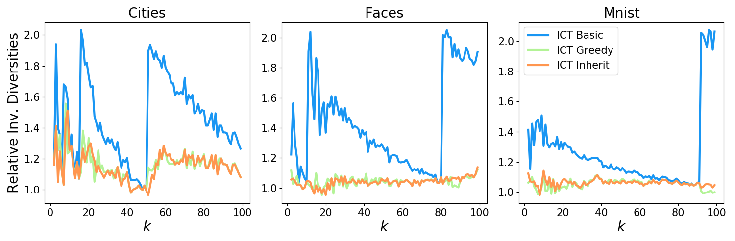
Figure 1: Achieved inverse diversities relative to GMM on the Cities, Faces and MNIST data set. Detailed setting of experiments is described in Section 4.

Recently, in many web applications including recommender systems, web search, and notification services, the diversification algorithm is required to handle streaming data, where the sample pool $V$ is dynamic—some new items can be added and some old items can be removed from time to time. Drosou and Pitoura (2014) [8] argued that the cover tree (CT), which was originally proposed for nearest neighbor search [3, 12], is an appropriate tool to meet those streaming requirements. In particular a family of CT approaches, called the incremental cover trees (ICTs), are suitable for dynamic diversification, because it allows addition and removal of items online. The authors reported excellent empirical performance. Especially, two variants, called ICT Greedy and ICT Inherit, typically provide a set with its diversity only $1/1.2$ times smaller than GMM (see Fig.1 for our experimental results).

Nevertheless, the theoretically known performance bound of ICT is $d^{*}/8$ [8], which is 4 times worse than GMM. The goal of this paper is therefore to fill this gap between theory and empirical observations. We theoretically analyze the property of ICT, and derive a tighter performance bound, $d^{*}/6$, for ICT Greedy and ICT Inherit. Then, we investigate the obtained bound and the empirical observations in details, by using specially designed artificial data for which the optimal diversity is known. Finally, we analyze the tightness of performance bounds, and show that our proposed bounds cannot be improved further, i.e., for worst case analysis, this paper gives the tightest possible bounds of all ICT variants. In addition, we demonstrate a new application of dynamic diversification for generative image samplers, where prototypes are incrementally collected from a stream of artificial images generated by an image sampler.

2 Background

As discussed already above, the $k$-max-min diversification problem is known to be NP-hard [18]. Therefore, various approximation algorithms have been proposed (see [13] for an overview). In order to assess the accuracy of their approximation, a theoretical bound on the worst possible performance is usually given.

Definition 2

[21] ($\alpha$-approximation algorithm) An $\alpha$-approximation algorithm for an optimization problem produces for all instances of the problem a solution whose value is within a factor $\alpha$ of the value of the optimal solution. $\alpha$ is called the approximation factor.

Let $S^{f}=f(V,k)$ be a diverse subset of $V$ of size $k$, which was computed using method $f$. $f$ is said to be an $\alpha$-approximation algorithm, iff for all possible diversification problems

$$div(S^{f})\geq d^{*}/\alpha,$$ (3)

where $d^{*}$ is the optimal diversity. Small values for $\alpha$ indicate better guaranteed performance, but because the approximate solution can at most be as good as the optimal solution, $\alpha\geq 1$. Along with the computational complexity, the approximation factor is an important criterion that theoretically guarantees the performance of an algorithm.

0:  $V$ - a set of points, $\;\;k$ - size of the subset

0:  $S$ - diverse subset of $V$ of size $k$

1:  $S\leftarrow$ randomly selected point $v\in V$

2:  while $|S|<k$ do

3:     $s^{*}\leftarrow\mathop{\mathrm{argmax}}_{v\in V\setminus S}\;\;\min_{s\in S}\;\;d(v,s)$

4:     $S\leftarrow S\cup\{s^{*}\}$

5:  end while

6:  return  $S$

Algorithm 1 Greedy Max-Min (GMM)

0:  $CT$ - a cover tree for data set $V$, $\;\;k$ - size of the subset

0:  $S$ - diverse subset of $V$ of size $k$

1:  $i\leftarrow i_{\max}$

2:  while $|C_{i}|<k$ do

3:     $i\leftarrow i-1$

4:  end while

5:  $S\leftarrow$ select $k$ nodes from $C_{i}$

6:  return  $S$

Algorithm 2 Cover Tree for $k$-Max-Min Diversification Problem

In this section we summarize GMM, one of the most established algorithms, and cover tree-based approaches. We give for each method the complexity and the approximation factor.

2.1 Greedy Max-Min (GMM) Algorithm

Although proposed several decades ago, greedy max-min (GMM) [18] is still state-of-the-art for the diversification problem. A detailed description of the algorithm can be found in Algorithm 1. GMM approximates the diverse subset in a greedy manner, starting with either a randomly selected data point (line 1) [1] or the two most distant data points of the set [18]. In subsequent iterations the data point with the largest pairwise distance to the current subset is added to the diverse set (line 3, 4). As the authors showed, GMM has an approximation factor $\alpha^{\mathrm{GMM}}$ of 2 and a complexity that is in $\mathcal{O}(N\cdot k)$.

2.2 Incremental Cover-tree (ICT) Approaches

Although, originally proposed for sublinear-time $k$-nearest neighbor search, the cover tree [4] can easily be adapted for diverse set approximation. A cover tree for a data set $V$ is a leveled tree such that each layer of the tree covers the layer beneath it. Every layer of the tree is associated with an integer level $i$, which decreases as we descend the tree. The lowest layer of the tree holds the whole data set $V$ and is associated with the smallest level $i_{\min}$, whereas the root of the tree is associated with the largest level $i_{\max}$. A node in the tree corresponds to a single data point in $V$, but a data point might map to multiple nodes. However, any point can only appear once in each layer. Let layer $C_{i}$ be the set of all nodes at level $i$. For all level $i$ with $i_{\min}\leq i\leq i_{\max}$, the following invariants must be met: (1) Nesting: $C_{i}\subseteq C_{i-1}$. Once a point $p\in V$ appears in $C_{i}$, every lower layer in the tree has a node associated with $p$. (2) Covering: For every $p\in C_{i-1}$, there exists a $q\in C_{i}$ such that $d(p,q)\leq b^{i}$ and the node in $C_{i}$ associated with $q$ is a parent of the node of $p$ in $C_{i-1}$. (3) Separation: For all distinct $p,q\in C_{i},d(p,q)>b^{i}$. Here $b>1$ denotes the base of the cover tree. The cover tree was proposed with $b=2$, but extended to arbitrary bases in [8] (cf. Fig. 8 in Appendix F for cover tree examples).

Due to the invariants, each layer of the tree might already be an useful approximation. The general procedure of using a cover tree for the $k$-max-min diversification problem, is shown in Algorithm 2. It aims to find the termination layer $C_{i}$ of the cover tree, i.e. the first layer that holds at least $k$ nodes. In general $|C_{i}|\geq k$, thus, a subset of nodes must be selected (line 5). Possible selection strategies were introduced in [8] and are presented below.

ICT Basic

ICT Basic is the most straight-forward approach. It randomly selects $k$ nodes out of $C_{i}$, with its complexity in $\mathcal{O}(k)$. Because of the random selection, the diversity of the subset computed with ICT Basic might be the same as the diversity of the whole termination layer.

ICT Greedy

ICT Greedy combines the cover tree approach with GMM. After the termination layer was located, we apply GMM on $C_{i}$ in order to select $k$ nodes. Compared to the purely random approach, this selection strategy will, in most cases, give results with higher diversity. By applying GMM only on $C_{i}$ instead of $V$, the complexity drastically reduces and is in $\mathcal{O}(|C_{i}|\cdot k)$.

ICT Inherit

0:  $CT$ - a cover tree for data set $V$, $\;\;k$ - size of the subset

0:  $S$ - diverse subset of $V$ of size $k$

1:  $i\leftarrow i_{\max}$

2:  while $|C_{i}|<k$ do

3:     $i\leftarrow i-1$

4:  end while

5:  $S\leftarrow C_{i+1}$

6:  while $|S|<k$ do

7:     $s^{*}\leftarrow\mathop{\mathrm{argmax}}_{c\;\in\;C_{i}\setminus\left(S\cup C_{i+1}\right)}\min_{s\in S}\;d(c,s)$

8:     $S\leftarrow S\cup\{s^{*}\}$

9:  end while

10:  return  $S$

Algorithm 3 Cover Tree Inherit

ICT Inherit is the most enhanced approach. It maintains the performance of ICT Greedy but further reduces the complexity. A detailed description can be found in Algorithm 3. Instead of applying GMM on the whole layer $C_{i}$, we initialize the diverse subset with the previous layer $C_{i+1}$ (line 5) and only select some nodes from the termination layer (line 6 to 9). Due to the separation invariant of the cover tree, $C_{i+1}$ already has a high diversity and, therefore, is an adequate initialization for the selection process. The complexity of ICT Inherit is in $\mathcal{O}\left(|C_{i}\setminus C_{i+1}|\cdot\left(k-|C_{i+1}|\right)\right)$.

2.2.1 Approximation Factor

In [8] a first attempt to estimate the approximation factor was made.

Proposition 1

[8] For $f\in\{\mathrm{ICTBasic},\mathrm{ICTGreedy},\mathrm{ICTInherit}\}$

$$\textstyle\alpha^{f}=\frac{2b^{2}}{b-1}.$$ (4)

For a cover tree built with $b=2$, this results in an approximation factor of $\alpha=8$, regardless of which selection strategy is used. However, as we will see in Sec. 3, a lower and tighter approximation factor for ICT Greedy and ICT Inherit can be proven.

2.3 Diversification of Dynamic Data

In many applications the set, for which a diverse subset is required, is not static. New data points must be added or old ones have to be removed from time to time. Unfortunately, GMM is not an adequate choice for the diversification of dynamic data. Whenever the data set $V$ is changed, GMM has to be rerun from scratch. Whereas the cover tree is a dynamic data structure. Insertion and removal of data points state no problem and the cover tree can easily be used for the diversification of dynamic data using the approaches presented above. Adding or removing a data point has complexity $\mathcal{O}(c^{6}\cdot N\log N)$ where $c$ is the expansion constant [4, 8].

3 Theoretical Analysis

Because of the cover tree properties, each layer of the cover tree might already be an appropriate starting point for the approximation of the diverse set. However, depending on the selection strategy, the quality of the diversity is likely to differ. We expect ICT Greedy and ICT Inherit to give results with higher diversity than ICT Basic. In the following we will prove that the approximation factor derived in [8] is only a loose bound when it comes to the GMM-based selection strategies.

Theorem 1

Let $C_{i}$ be the termination layer, i.e. the first layer of the cover tree that holds at least $k$ nodes

$$\forall j>i,|C_{j}|<k,$$ (5)

and $\beta\in\mathbb{R}^{+}$ be defined, such that

$$\textstyle b^{i}=\frac{d^{*}}{\beta}.$$ (6)

The diversity of every subset of $C_{i}$ can be bounded

$$\forall\;C\subseteq C_{i}\,:\,{div}\left(C\right)\geq\frac{d^{*}}{\beta}.$$ (7)

Furthermore, $C_{i}$ will hold a subset $C$ of $k$ nodes with diversity of at least

$$\textstyle\exists\;C\subseteq C_{i},|C|=k\,:\,{div}\left(C\right)\geq\max\left\{\frac{d^{*}}{\beta},d^{*}(1-\frac{1}{\beta}\frac{2b}{b-1})\right\}$$ (8)

and $\beta<\frac{2b^{2}}{b-1}$. It follows

$$\textstyle\frac{d^{*}}{div(C)}\leq 1+\frac{2b}{b-1}.$$ (9)

We give a sketch of the proof. For a detailed discussion see Appendix B. Eq. (7) and the first part of the maximum in Eq. (8) follows from the separation property of the cover tree. The latter part of the maximum follows from the covering and nesting property. Any layer of the cover tree covers the whole data set. As a consequence $C_{i}$ is guaranteed to hold a subset of nodes, that cover the optimal diverse set. The triangle inequality can then be used, to bound the distance between those nodes. This gives rise to the existence of $C$ and the latter part of the maximum. $\Box$

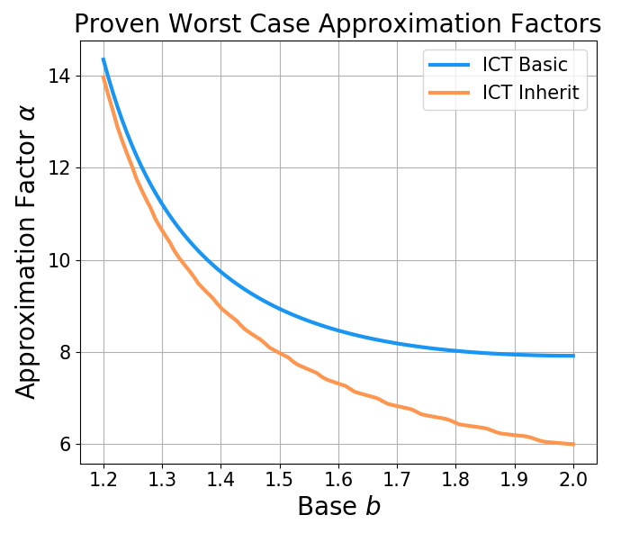
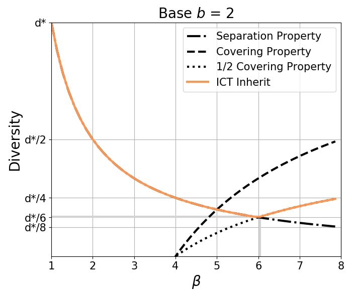
Figure 2: Visualization of the theoretical bounds derived in Sec. 3. (left) Guaranteed approximation factor for ICT Basic and ICT Inherit for different values of the base $b$. ICT Greedy has the same approximation factor as ICT Inherit. (right) The bound on the diversity derived in Eq. (8) for various values of $\beta$ and $b=2$. Separation Property shows the first part of the maximum and Covering Property shows the latter part of the maximum. The intercept of both lines shows what is stated in Eq. (9). The worst case approximation factor is 6.

For some $\beta$ it is crucial to select a subset of $C_{i}$ in an appropriate manner. Thus, the diversity strongly depends on the strategy, that is used to select $k$ nodes out of $C_{i}$.

Corollary 1

Let $S^{\mathrm{ICTGreedy}}\subseteq C_{i}$ be a subset of $k$ nodes selected from $C_{i}$ using GMM (ICT Greedy). The diversity of $S^{\mathrm{ICTGreedy}}$ is at least

$$\textstyle div\left(S^{\mathrm{ICTGreedy}}\right)\geq\text{max}\left\{\frac{d^{*}}{\beta},\frac{1}{2}\,d^{*}(1-\frac{1}{\beta}\frac{2b}{b-1})\right\}.$$ (10)

The approximation factor $\alpha$ of ICT Greedy is given by

$$\textstyle\frac{d^{*}}{div(S^{\mathrm{ICTGreedy}})}\leq 2+\frac{2b}{b-1}=\alpha^{\mathrm{ICTGreedy}}.$$ (11)

For a detailed proof see Appendix C. The diversity of the selected subset cannot be worse than $\nicefrac{{d^{*}}}{{\beta}}$, because that bound is given by the separation criterion. As it was shown in [18], GMM has an approximation factor of $2$. The best possible diversity in layer $C_{i}$ is given by Eq. (8). We get what is stated in Eq. (10). $\Box$

For $b=2$, this results in an approximation factor of $\alpha^{\mathrm{ICTGreedy}}=6$. Compared to ICT Greedy, ICT Inherit has a lower complexity. Moreover, ICT Inherit has the same bound on the diversity and the same approximation factor.

Theorem 2

Let $S^{\mathrm{ICTInherit}}\subseteq C_{i}$ be a subset of $k$ nodes selected from $C_{i}$. It holds all nodes from the previous layer $C_{i+1}$ and remaining nodes were selected from $C_{i}\setminus C_{i+1}$ using GMM (ICT Inherit). The bound of the diversity of $S^{\mathrm{ICTInherit}}$ is the same as the bound for $div\left(S^{\mathrm{ICTGreedy}}\right)$, i.e.

$$\textstyle div\left(S^{\mathrm{ICTInherit}}\right)\geq\max\left\{\frac{d^{*}}{\beta},\frac{1}{2}\,d^{*}(1-\frac{1}{\beta}\frac{2b}{b-1})\right\}.$$ (12)

The approximation factor $\alpha$ of ICT Inherit is given by

$$\textstyle\frac{d^{*}}{div(S^{\mathrm{ICTInherit}})}\leq 2+\frac{2b}{b-1}=\alpha^{\mathrm{ICTInherit}}.$$ (13)

For a detailed proof, see Appendix D. Instead of starting with a randomly selected data point, ICT Inherit initializes GMM with $C_{i+1}$. An approximation factor of 2 for GMM was proven by induction in [18]. In order to prove that initializing GMM still leads to an approximation factor of 2, it is thus sufficient to show the minimum pairwise distance in $C_{i+1}$ is larger than or equal to half of the optimal diversity of $C_{i}$. Because of the separation property of the cover tree, the nodes in $C_{i+1}$ are guaranteed to have larger pairwise distance than the nodes in $C_{i}$. Using also the nesting property $C_{i+1}\subseteq C_{i}$, we can conclude that $div\left(C_{i+1}\right)$ is sufficiently large. $\Box$

Figure 2 (left) shows the approximation factor for different bases $b$. Especially for $b=2$, using ICT Greedy or ICT Inherit as selection strategy reduces the approximation factor. Figure 2 (right) shows the bound on the diversity derived in Eq. (8). One can see, for small $\beta$ the diversity of the subset is given by the separation criterion. This can also be explained intuitively. As $\beta$ increases, the pairwise distance that is bounded by the separation criterion decreases. However, the cover radius $b^{i}$ of each node decreases as well, so that at least $k$ nodes in $C_{i}$ must lie close to the data points in the optimal solution to be able to cover them. Therefore, the pairwise distance of those nodes increases as $\beta$ decreases. When the termination layer corresponds to a lower level of the tree (larger $\beta$), it is beneficial to use a GMM-based selection strategy. The minimum of both bounds corresponds to the approximation factor.

4 Tightness of Performance Bounds

According to our theory in Section 3, the approximation factor of ICT methods are $\alpha^{\mathrm{ICTBasic}}=8$, $\alpha^{\mathrm{ICTGreedy}}=\alpha^{\mathrm{ICTInherit}}=6$ for $b=2$. In this section, we investigate if these bounds are tight or whether there is still room for improvement. We first conducted an artificial data experiment, designed for validating our theory. We created a set of data points consisting of grid points and random points (see Fig. 3 for examples). For $k$ equal to the number of grid points, the optimal diverse subset is given by the grid.

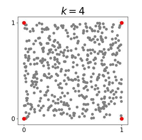
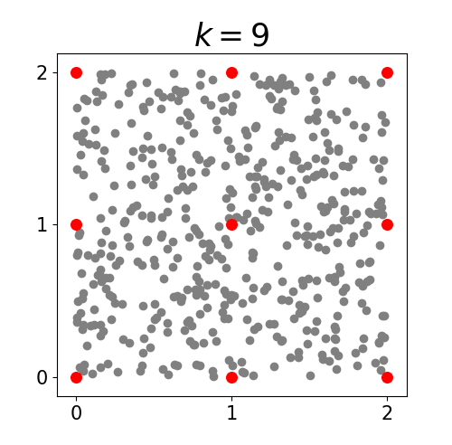
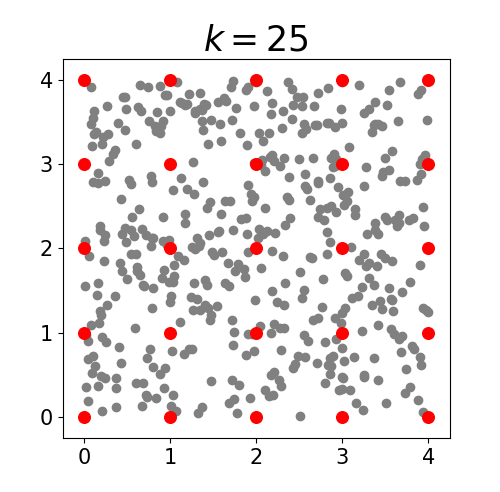
Figure 3: 2D artificial data consisting of $2\times 2$ (left), $3\times 3$ (center) or $5\times 5$ grid points (right) and random, uniformly distributed points. The optimal diversity is $d^{*}=1.0$.

Using the methods presented above, we approximate the diverse subsets and computed the relative inverse diversity $\nicefrac{{d^{*}}}{{S^{f}}}$ for $f\in\{\mathrm{GMM},\mathrm{ICTBasic},\mathrm{ICTGreedy},\mathrm{ICTInherit}\}$. According to Eq. (3), the computed rel. inv. diversity can at most be as large as the approximation factor and small rel. inv. diversity indicate better results. By repeating the experiments (100 trials each), we were able to estimate the distribution of the rel. inv. diversity. Figure 4 shows the result on the 2D and 5D grid data for base $b$ set to $2$.

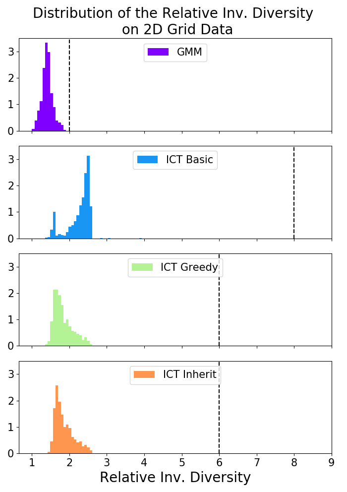
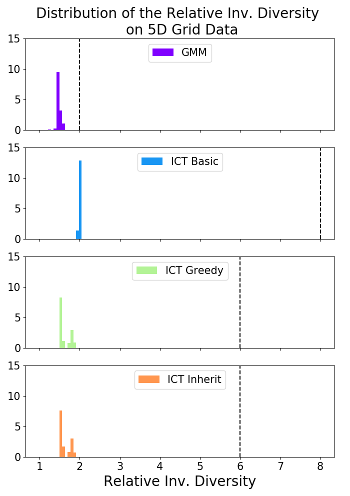
Figure 4: Estimated distribution of the relative inverse diversity on the 2D (left) and 5D (right) grid data. The cover tree was built with $b=2$. The dashed vertical lines indicate the proven approximation factor.

We still observe a big gap between the theoretical bounds and empirical observations. Although GMM has an approximation factor that is three times lower than the guaranteed approximation factor of ICT Greedy and ICT Inherit with $b=2$, only minor differences can be seen. One can see, that the center of the distribution of the observed rel. inv. diversity is even lower than 2. The highest observed rel. inv. diversity was $2.9$ for ICT Inherit, $2.6$ for ICT Greedy and $3.9$ for ICT Basic on the 2D data set. Note that for larger $k$, we tend to select nodes from lower layers of the tree. Lower layers hold more, but evenly spaced nodes, because their cover radius $b^{i}$ is smaller. This might explain the excellent performance on the 5D grid data.

The approximation factor is defined as an upper bound. Thus, when an approximation factor is proven, it does not imply, that no smaller approximation factor is possible. Because of the high performance of the cover tree approaches on the grid data sets, one might expect lower approximation factors, than the ones that were proven in Sec. 3. However, we provide two examples, that show the tightness of $\alpha^{\mathrm{ICTBasic}}$, $\alpha^{\mathrm{ICTGreedy}}$ and $\alpha^{\mathrm{ICTInherit}}$ (see Appendix E). Thereby, we have shown that no lower approximation factor can be proven. Note, that the rel. inv. diversity does not only depend on the data pool, but also on the order in which the data is added to the tree. Even for the examples, which are discussed in the Appendix, we only get the worst case rel. inv. diversity, if the data points are added in a specific order. When this order is changed, we might also get the optimal diverse set. See the Appedendix A for the incremental insertion algorithm of the cover tree. With the excellent performance on the artificial data and this observation at hand, we can conclude, that observing the worst possible rel. inv. diversity is highly unlikely, but not impossible.

We also conducted real world data experiments - both high dimensional and large sample sized. Cities [5] consists of the latitude and longitude of cities in Europe. Faces [2] consists of 60x64 grey-scale images of people taken with varying pose and expressions. MNIST [14] holds 28x28 images of handwritten digits. For each of the data sets we ran GMM and the cover tree approaches (built with $b=2$) with varying diverse set sizes ($k\in[2,100]$). In general the optimal diversity is unknown. Therefore, we plotted the inverse diversity relative to the diversity of GMM, i.e., $\nicefrac{{div(S^{GMM})}}{{div(S^{f})}}$, where $f\in\{\mathrm{ICTBasic},\mathrm{ICTGreedy},\mathrm{ICTInherit}\}$ corresponds to the applied method. This can be used to bound the true rel. inv. diversity. If, for example, $\nicefrac{{div(S^{GMM})}}{{div(S^{\mathrm{ICTInherit}})}}=1.5$, we can conclude $\nicefrac{{d^{*}}}{{div(S^{\mathrm{ICTInherit}})}}\leq 3$, because GMM has an approximation factor of 2.

Figure 1 shows the inv. diversity relative to the diversity of GMM on the Cities, Faces and MNIST data set. ICT Greedy, ICT Inherit and GMM compute subsets with diversities of almost the same magnitude. Even ICT Basic gives results with high diversity. Note, that the inv. diversity relative to GMM of ICT Basic resembles a step-function. This can be explained by the layer-wise structure of the cover tree. When $k$ is small compared to the number of nodes in the termination layer, ICT Basic might select poorly which results in lower diversity than ICT Inherit. As $k$ approaches the size of the layer, both approaches will select similar subsets.

5 Application to Image Generator

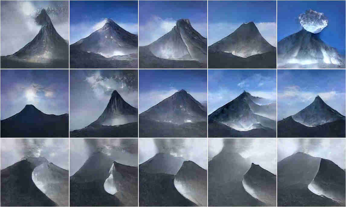
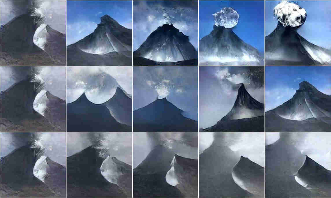
Figure 5: $k=5$ randomly chosen images (left) from the MCMC sequence of PPGN for Volcano class, and the corresponding diverse sets (right) chosen by ICT Inherit, after 20 (bottom), 100 (middle), and 200 (top) MCMC steps.

As a new use of dynamic diversification, we applied ICT Inherit to sequentially collect a diverse set from the MCMC image sequence generated by the plug and play generative networks (PPGN) [17], which have shown to provide highly diverse realistic images with high resolution. For generated images by MCMC sampling, there is strong correlation between subsequent images. One needs to cherry-pick diverse images by hand, or generate a long sequence and randomly choose images from it, to show how diverse the images are, that a new sampling strategy generates. Dynamic diversification by ICT Inherit can automate this process, and might be used as a standard tool to assess the diversity of samplers.

Fig.5 shows images of the Volcano class generated by PPGN. We ran PPGN up to 200 steps, adding a new image to ICT Inherit in each step. In the right half of Fig.12, we show the $k=5$ diverse images after 20 (bottom row), 100 (middle row), and 200 (top row) steps of image generation. For comparison, we show randomly chosen images in the left half. We can see that ICT Inherit successfully chose more diverse images than the random choice. More examples for other classes are shown in Appendix G.

6 Conclusion

Selecting a diverse subset of a dynamic sample pool—dynamic diversification—is a common problem in many machine learning applications. The diversification problem is known to be NP-hard, but polynomial time approximation algorithms, such as greedy max-min (GMM) algorithm, can have an approximation factor of 2, i.e., they are guaranteed to give a solution with diversity larger than half of the optimal diversity. However, GMM has to be performed from scratch every time the sample pool is updated, e.g., new items are added or old items are removed, and therefore is not suitable for dynamic diversification. Previous work argued that cover trees, originally proposed for nearest neighbor search, could be adapted for dynamic diversification, and proposed ICT Basic, ICT Greedy and ICT Inherit, which gave results only marginally worse than the results of GMM, while the approximation factor of those approaches was assumed to be four times larger.

In this work we have conducted both theoretical analyses and extensive experiments to fill the gap between the theoretical bound and empirical observation. Specifically, we could prove a tighter approximation factor for ICT Greedy and ICT Inherit, reducing it to 6 instead of 8 for a cover tree with base $b=2$. Through artificial experiment, we have validated the bounds, and assessed the tightness of the bounds. Even on real world data sets, all three cover tree approaches give excellent results, with diversities almost of the same magnitude as the diversity given by GMM. The performance of the cover tree approaches is remarkably higher than the theoretical approximation factor, which might imply that our bounds are still loose. However, we found worst case examples that achieve the theoretical approximation factor, which proves that our bounds for ICT are tightest possible.

In general, the diversity of subsets computed with one of the cover tree approaches does not only depend on the data pool, but also on the order in which the data is added to the tree. Therefore, we conclude, that observing the worst possible relative inverse diversity is highly unlikely. Further effort must be made to assess how likely cover tree approaches give solutions with worst possible diversity.

Finally, our demonstration of dynamic diversification for generative image samplers shows the high potential of our theoretical insight for practical applications. Future work will also study diversification in scientific applications, where systematically creating a diverse (and therefore representative) subset of large data corpora can lead to novel insight, e.g. in molecular dynamics or sampling applications in chemistry.

Acknowledgments

The authors thank Vignesh Srinivasan of Fraunhofer HHI for discussion on the image generator application. This work was supported by the German Research Foundation (GRK 1589/1) by the Federal Ministry of Education and Research (BMBF) under the project Berlin Big Data Center (FKZ 01IS14013A).

Appendix A Incremental Insertion

Algorithm 4 shows how a data point $p$ can be inserted in an existing cover tree. It is based on the insertion algorithm in [4], which was extended to arbitrary bases in [8]. We reduced the complexity of the algorithm by omitting the nearest-parent heuristic.

0:  $p$ - data point $\;\;\;Q_{i}$ - subset of nodes of layer $i$ of the cover tree

0:  Cover tree with $p$ inserted

1:  $C\leftarrow\left\{children(q)|q\in Q_{i}\right\}$

2:  if $\min_{c\in C}d(p,c)>b^{i}$ then

3:     return  true

4:  else

5:     $Q_{i-1}\leftarrow\left\{c\in C|d(p,c)\leq\frac{b^{i}}{b-1}\right\}$

6:     flag $\leftarrow$ Insert$(p,Q_{i-1},i-1)$

7:     if flag and $d(p,Q_{i})\leq b^{i}$ then

8:        $q^{*}\leftarrow$ choose node in $Q_{i}$ as parent

9:        make $p$ a child of $q^{*}$

10:        return  false

11:     else

12:        return  flag

13:     end if

14:  end if

Algorithm 4 Insert($p$, $Q_{i}$, $i$)

We start with the root layer Insert$(p,C_{i_{max}},i_{max})$ and traverse the cover tree until we find the first layer such that $p$ is separated from all other nodes (line 2). Only the nodes that can cover $p$ are considered in each iteration ($Q_{i}$). When we found an appropriate layer (line 7), we add $p$ as a child to one node in $Q_{i}$ (line 8,9).

Appendix B Proof of Theorem 1

B.1 Bound on $\beta$

Recall (Eq. (6)), that $\beta$ is defined as the fraction of the optimal diversity and the cover radius of the termination layer. Because the optimal solution is not known, the exact value of $\beta$ can in general not be identified. We will use the properties of the cover tree to give a bound on possible values of $\beta$. We first consider how $\beta$ must be chosen, so that $C_{i}$ holds at least $k$ nodes. To do so, assume we try to enclose, two data points $p$ and $p^{\prime}$ with $d(p,p^{\prime})=d^{*}$ with one ball. A single ball won’t be able to enclose those two data points, if its radius is less than $\nicefrac{{d^{*}}}{{2}}$. No matter where the ball is placed, the maximal distance it can enclose is less than $2\cdot\nicefrac{{d^{*}}}{{2}}$ and thus, smaller than the distance between $p$ and $p^{\prime}$. Because it holds for any pair of data points, the same will hold for the general case of $k$ data points. If the pairwise distance between two data points is at least $d^{*}$, any ball with radius less than $\nicefrac{{d^{*}}}{{2}}$ can only enclose one of those $k$ data points at once. Thus, we need at least $k$ balls to enclose $k$ data points.

Let $desc(c)$ denote the the set of descendants of node $c$. We say, that a node $c$ covers a node $v$, if $v\in desc(c)$. Furthermore, we say that a layer $C$ of the cover tree covers a set of nodes $C^{\prime}$, if

$$C^{\prime}\subseteq\left(\bigcup_{c\in C}desc(c)\right).$$ (14)

As a consequence of the covering and the nesting property, each layer of the cover tree does not only cover the layer beneath it, but covers the whole data set $V$, i.e.

$$\forall i\in[i_{\min},i_{\max}]\,:\left(\bigcup_{c\in C_{i}}desc(c)\right)=V.$$ (15)

Let $S^{*}\subseteq V$ with $div(S^{*})=d^{*}$ denote the optimal diverse set. Because $S^{*}$ is a subset of $V$, $C_{i}$ will cover the optimal solution i.e.

$$S^{*}\subseteq\bigcup_{c\in C_{i}}desc(c).$$ (16)

The maximal distance to any descendant of any node $c\in C_{i}$ can be bounded

$$\forall c\in C_{i},\forall v\in desc(c):d(c,v)<\frac{b^{i+1}}{b-1}=\frac{d^{*}}{\beta}\frac{b}{b-1}.$$ (17)

Thus, if the maximal distance to any descendant is less than $\nicefrac{{d^{*}}}{{2}}$, any node $c$ in $C_{i}$ will only be able to cover one of the optimal data points in $S^{*}$. Because $|S^{*}|=k$, $C_{i}$ is guaranteed to hold at least $k$ nodes, if

$$\frac{b^{i+1}}{b-1} \leq\frac{d^{*}}{2}$$ (18)

$$\Leftrightarrow\frac{d^{*}}{\beta}\frac{b}{b-1} \leq\frac{d^{*}}{2}$$ (19)

$$\Leftrightarrow\frac{2b}{b-1} \leq\beta$$ (20)

(we can use $\leq$ instead of strict inequality, because $\nicefrac{{b^{i+1}}}{{b-1}}$ is already a strict upper bound for the distance to the descendants).

We have shown, that $C_{i}$ will hold at least $k$ data points, if $b^{i}\leq d^{*}\cdot\nicefrac{{b-1}}{{2b}}$. Note, that the cover tree might already hold $k$ nodes in an higher layer, especially because $C_{i}$ must not only cover $S^{*}$ but the whole data set $V$. In those cases, the diversity of the solution will be higher (separation criterion).

This property can be used to find an upper bound for $\beta$. Assume $C_{i}$ is the termination layer and $b^{i}=d^{*}\cdot\nicefrac{{b-1}}{{2b^{2}}}$. In that case $b^{i+1}=b\cdot d^{*}\cdot\nicefrac{{b-1}}{{2b^{2}}}=d^{*}\cdot\nicefrac{{b-1}}{{2b}}$. However, as shown above, this implies that $C_{i+1}$ holds at least $k$ nodes. Thus, $C_{i}$ cannot be the termination layer, because $C_{i+1}$ would have been. We can conclude

$$\beta<\frac{2b^{2}}{b-1}.$$ (21)

B.2 Bound on the Diversity

We prove each part of the maximum in Eq. (8) individually. The first part follows immediately from the separation criterion and the definition of $\beta$. Any subset of $C_{i}$ will have a diversity of at least $\nicefrac{{d^{*}}}{{\beta}}$,

$$\forall c,c^{\prime}\in C_{i},d(c,c^{\prime})>b^{i}\Rightarrow div(C_{i})>\frac{d^{*}}{\beta}.$$ (22)

In order to prove the second part of the maximum, we assume every data point of the optimal solution is covered by a single node in $C_{i}$, i.e. $\beta\geq\nicefrac{{2b}}{{b-1}}$. Let $c,c^{\prime}\in C_{i}$ be an arbitrary pair of nodes in the termination layer which covers $p,p^{\prime}\in S^{*}$. Without loss of generality we assume $c$ covers $p$, $c^{\prime}$ covers $p^{\prime}$ and $d(p,p^{\prime})\geq d^{*}$. Because of the covering property

$$d(c,p) <\frac{b^{i+1}}{b-1}=\frac{d^{*}}{\beta}\frac{b}{b-1}$$ (23)

$$d(c^{\prime},p^{\prime}) <\frac{b^{i+1}}{b-1}=\frac{d^{*}}{\beta}\frac{b}{b-1}.$$ (24)

Using the triangle inequality, we get

$$d(p,c)+d(c,p^{\prime}) \geq d(p,p^{\prime})$$ (25)

$$d(p,c)+d(c,c^{\prime})+d(c^{\prime},p^{\prime}) \geq d(p,p^{\prime})$$ (26)

$$d(c,c^{\prime}) \geq d(p,p^{\prime})-d(p,c)-d(c^{\prime},p^{\prime})$$ (27)

$$d(c,c^{\prime}) >d^{*}-\frac{d^{*}}{\beta}\frac{b}{b-1}-\frac{d^{*}}{\beta}\frac{b}{b-1}$$ (28)

$$d(c,c^{\prime}) >d^{*}(1-\frac{1}{\beta}\frac{2b}{b-1}).$$ (29)

Because any data point of the optimal solution is by assumption covered by one node in $C_{i}$ and the pairwise distance of those data points is at least $d^{*}$, it follows that $C_{i}$ holds a subset of $k$ nodes, that have pairwise distance of at least $d^{*}(1-\nicefrac{{1}}{{\beta}}\cdot\nicefrac{{2b}}{{b-1}})$.

Recall, that we assumed $\beta\geq\nicefrac{{2b}}{{b-1}}$ in the beginning of the second part of the proof, to make sure that every data point of the optimal solution is covered by a different node of the termination layer. This does not impose any restrictions on the validity of the bound, because for $\beta<\nicefrac{{2b}}{{b-1}}$, $\text{max}\left\{\nicefrac{{d^{*}}}{{\beta}},\,d^{*}(1-\nicefrac{{1}}{{\beta}}\cdot\nicefrac{{2b}}{{b-1}})\right\}=\nicefrac{{d^{*}}}{{\beta}}$ and the overall bound still holds. This concludes the proof of the theorem.

B.3 Fraction of Diversities

First note, that $\nicefrac{{d^{*}}}{{\beta}}$ decreases and $d^{*}\cdot(1-\nicefrac{{1}}{{\beta}}\cdot\nicefrac{{2b}}{{b-1}})$ increases as $\beta$ increases. As a consequence, the bound of the diversity in Eq. (8) is minimal, when

$$\frac{d^{*}}{\beta}=d^{*}(1-\frac{1}{\beta}\frac{2b}{b-1}).$$ (30)

Solving for $\beta$ leads to

$$\frac{1}{\beta} =1-\frac{1}{\beta}\frac{2b}{b-1}$$ (31)

$$\frac{1}{\beta}(1+\frac{2b}{b-1}) =1$$ (32)

$$1+\frac{2b}{b-1} =\beta.$$ (33)

We use this minimum and give a bound on the fraction of the diversities

$$\frac{d^{*}}{div(C)} \leq\frac{d^{*}}{\min_{\beta}\left\{\max\left\{\frac{d^{*}}{\beta},d^{*}(1-\frac{1}{\beta}\frac{2b}{b-1})\right\}\right\}}$$ (34)

$$=\frac{d^{*}}{\frac{d^{*}}{1+\frac{2b}{b-1}}}$$ (35)

$$=1+\frac{2b}{b-1}.$$ (36)

Appendix C Proof of Corollary of Theorem 1

Suppose we use ICT Greedy to select a subset of $k$ nodes from $C_{i}$. The diversity of the selected subset cannot be worse than $\nicefrac{{d^{*}}}{{\beta}}$, because that bound is given by the separation criterion. As it was shown in [18], GMM has an approximation factor of $2$. We select $k$ nodes from $C_{i}$ not from $V$ itself. Thus, the best possible diversity is not $d^{*}$, but rather given by Eq. (8), i.e. the optimal diversity in layer $C_{i}$. We get what is stated in Eq. (10).

As it was shown in [18], the complexity of GMM is in $\mathcal{O}(N\cdot k)$ where $N$ is the size of the set, from which $k$ data points are selected. Here we select data points from the termination layer, i.e. $N=|C_{i}|$. Analogous to what was shown in Sec. B.3, we can prove the approximation factor of ICT Greedy. Solving

$$\frac{d^{*}}{\beta}=\frac{1}{2}\,d^{*}(1-\frac{1}{\beta}\frac{2b}{b-1})$$ (37)

for $\beta$ leads to

$$\beta=2+\frac{2b}{b-1}.$$ (38)

Again, we use this value for the calculation of the minimum of $div(S^{\mathrm{ICTGreedy}})$

$$\frac{d^{*}}{div(S^{\mathrm{ICTGreedy}})} \leq\frac{d^{*}}{\min_{\beta}\left\{\max\left\{\frac{d^{*}}{\beta},\frac{1}{2}d^{*}(1-\frac{1}{\beta}\frac{2b}{b-1})\right\}\right\}}$$ (39)

$$=\frac{d^{*}}{\frac{d^{*}}{2+\frac{2b}{b-1}}}$$ (40)

$$=2+\frac{2b}{b-1}.$$ (41)

Appendix D Proof of Theorem 2

ICT Inherit uses GMM to calculate a subset of layer $C_{i}$. Instead of starting with a randomly selected data point (as in GMM or ICT Greedy resp.), we start with $C_{i+1}$ and subsequently add new data points. The proof of the approximation factor of GMM relies on induction, thereby it was shown that the approximation factor holds after each iteration (see [18] for more details). Once it is shown that $C_{i+1}$ does not contradict an approximation factor of 2, the remaining proof in [18] can simply be applied. Thus, we show for any possible value of $\beta$ the minimum possible pairwise distance in $C_{i+1}$ is larger than or equal to half of the optimal diversity in $C_{i}$. Because the diversity of $C_{i}$ can at most be as large as the optimal diversity, $\beta\geq 1$ (recall Eq. (7)). As it was stated in the first theorem, $\beta<\nicefrac{{2b^{2}}}{{b-1}}$. According to the separation criterion

$$\forall c,c^{\prime}\in C_{i+1},d(c,c^{\prime})>b^{i+1}=b\cdot\frac{d^{*}}{\beta}$$ (42)

and thus, we show

$$\forall\beta\in\left[1,\frac{2b^{2}}{b-1}\right[\;.\;b\cdot\frac{d^{*}}{\beta}\geq\text{max}\left\{\frac{d^{*}}{\beta},\frac{1}{2}\,d^{*}(1-\frac{1}{\beta}\frac{2b}{b-1})\right\}.$$ (43)

• $\text{max}\left\{\frac{d^{*}}{\beta},\frac{1}{2}\,d^{*}(1-\frac{1}{\beta}\frac{2b}{b-1})\right\}=\frac{d^{*}}{\beta}$

  $$b\cdot\frac{d^{*}}{\beta}\geq\frac{d^{*}}{\beta}$$ (44)

  holds, since $b>1$.

• $\text{max}\left\{\frac{d^{*}}{\beta},\frac{1}{2}\,d^{*}(1-\frac{1}{\beta}\frac{2b}{b-1})\right\}=\frac{1}{2}\,d^{*}(1-\frac{1}{\beta}\frac{2b}{b-1})$

  $$b\cdot\frac{d^{*}}{\beta} \geq\frac{1}{2}\,d^{*}(1-\frac{1}{\beta}\frac{2b}{b-1})$$ (45)

  $$b\cdot\frac{d^{*}}{\beta} \geq\frac{1}{2}d^{*}-\frac{d^{*}}{\beta}\frac{b}{b-1}$$ (46)

  $$b\cdot\frac{1}{\beta} \geq\frac{1}{2}-\frac{1}{\beta}\frac{b}{b-1}$$ (47)

  $$b+\frac{2b}{b-1} \geq\frac{\beta}{2}$$ (48)

  $$2b+\frac{4b}{b-1} \geq\beta$$ (49)

  $$\frac{2b\cdot(b+1)}{b-1} \geq\beta$$ (50)

  holds for $\beta\in\left[1,\frac{2b^{2}}{b-1}\right[$.

Thus,

$$div(C_{i+1})\geq\text{max}\left\{\frac{d^{*}}{\beta},\frac{1}{2}\,d^{*}(1-\frac{1}{\beta}\frac{2b}{b-1})\right\}$$ (52)

which was to be shown.

When GMM is initialized with $C_{i+1}$ it only has to select $k-|C_{i+1}|$ data points. It is easy to see that the complexity reduces. In the first iteration, the distances from each data point in $C_{i+1}$ to every data point in $C_{i}\setminus C_{i+1}$ is computed in order to find the next data point. In each subsequent iteration, only the distance between the data point which was selected in the last iteration and the remaining available data set is computed. In total, ICT Inherit performs

$$\left(|C_{i}\setminus C_{i+1}|\cdot(k-|C_{i+1}|)\right)+\sum_{m=1}^{k-|C_{i+1}|-1}\left(|C_{i}\setminus C_{i+1}|-m\right)$$ (53)

distance computations and has therefore a complexity of $\mathcal{O}\left(|C_{i}\setminus C_{i+1}|\cdot\left(k-|C_{i+1}|\right)\right)$.

Because ICT Inherit has the same bound on the diversity as ICT Greedy (cf. (10) and (12)), both approaches have the same approximation factor.

Appendix E Tightness of the Proven Approximation Factors

The approximation factor is defined as an upper bound. Thus, when an approximation factor is proven, it does not imply, that no smaller approximation factor is possible. In this section we give two examples, that show the tightness of the derived approximation factors for arbitrary bases and $k=2$.

E.1 Tightness of $\alpha^{\mathrm{ICTBasic}}$

Let the data set be defined as

$$V=\left\{\left(\begin{array}[]{c}v\\ 0\\ \end{array}\right),\left(\begin{array}[]{c}0\\ b+\mu\\ \end{array}\right)|v\in\pm\left(\{0\}\;\cup\;\left(\bigcup_{J\in[1,J_{max}]}\left\{\sum_{j=1}^{J}b^{2}\cdot{\left(\frac{1}{b}\right)}^{j-1}\right\}\right)\;\cup\;\left\{\frac{b^{3}}{b-1}-\eta\right\}\right)\right\},$$ (54)

where $\mu,\eta>0$ small and $J_{max}$ be the smallest integer such that

$$\frac{b^{3-J_{max}}}{b-1}-b^{i_{min}+1}\leq\eta.$$ (55)

Most of the data points in $V$ lie on the line between ${(-\frac{b^{3}}{b-1}+\eta,0)}^{T}$ and ${(\frac{b^{3}}{b-1}-\eta,0)}^{T}$, where the distance between neighboring data points decreases as we move to the ends of the line. Only the data point ${(0,b+\mu)}^{T}$ does not lie on that line, but above the midpoint ${(0,0)}^{T}$. We choose the Euclidean distance as distance metric. The optimal solution $S^{*}\subseteq V$ for $k=2$ is given by

$$S^{*}=\{{(-\frac{b^{3}}{b-1}+\eta,0)}^{T},{(\frac{b^{3}}{b-1}-\eta,0)}^{T}\}$$ (56)

with a diversity of

$$d^{*}=2\frac{b^{3}}{b-1}-2\eta\;\;\approx\;\;2\frac{b^{3}}{b-1}.$$ (57)

The cover tree for $V$ is built with base $b$ such that data points are incrementally added, ordered according to their absolute $x$ value. As a result, we get the following cover tree:

• $i_{max}$: $C_{i_{max}}=\left\{{\left(0,0\right)}^{T}\right\}$

• $i=1$: $C_{i}=C_{i+1}\cup\left\{{(0,b+\mu)}^{T},-b^{2},b^{2}\right\}$

• $1>i>i_{min}$: $C_{i}=C_{i+1}\cup\left\{{\left(-\sum_{j=1}^{i_{max}-i}b^{2}\cdot{\left(\frac{1}{b}\right)}^{j-1},0\right)}^{T},{\left(\sum_{j=1}^{i_{max}-i}b^{2}\cdot{\left(\frac{1}{b}\right)}^{j-1},0\right)}^{T}\right\}$

• $i_{min}$: $C_{i_{min}}=C_{i_{min}+1}\cup\left\{{(-\frac{b^{3}}{b-1}+\eta,0)}^{T},{(\frac{b^{3}}{b-1}-\eta,0)}^{T}\right\}$

The data point ${\left(0,0\right)}^{T}$ will be the root node and each lower layer of the tree will hold the next two outer data points on the line. $i_{max}$ must be large enough so that the root is able to cover even the most distant data points, i.e. the optimal solution.

$$\frac{b^{i_{max}+1}}{b-1} >\frac{b^{3}}{b-1}-\eta$$ (58)

$$\frac{b^{i_{max}+1}}{b-1} \geq\frac{b^{3}}{b-1}$$ (59)

$$i_{max}\geq 2$$ (60)

For simplicity, we assume $i_{max}=2$ (any layer above $i=2$ will hold only the root). The layer with $i_{min}=i_{max}-J_{max}-1$ will hold the whole data set $V$. Because the distance between any data point in $V$ and ${(0,b+\mu)}^{T}$ is larger than $b^{1}$, there will be a node for ${(0,b+\mu)}^{T}$ in layer $i=1$. We will proof the cover tree properties to show that this is a valid cover tree. (1) Nesting: Obviously holds, as $C_{i+1}\subseteq C_{i}$. (2) Covering: Holds for $i=1$, because the maximal distance of any point in $C_{1}$ to the root ${\left(0,0\right)}^{T}$ is $b^{2}=b^{i_{max}}$. Let $1>i>i_{min}$ be an arbitrary level. The nodes ${\left(-\sum_{j=1}^{i_{max}-i-1}b^{2}\cdot{\left(\frac{1}{b}\right)}^{j-1},0\right)}^{T}$ and ${\left(\sum_{j=1}^{i_{max}-i-1}b^{2}\cdot{\left(\frac{1}{b}\right)}^{j-1},0\right)}^{T}$ are the parents of the nodes ${\left(-\sum_{j=1}^{i_{max}-i}b^{2}\cdot{\left(\frac{1}{b}\right)}^{j-1},0\right)}^{T}$ and ${\left(\sum_{j=1}^{i_{max}-i}b^{2}\cdot{\left(\frac{1}{b}\right)}^{j-1},0\right)}^{T}$. Their distance can be computed as

$$d\left({\left(\sum_{j=1}^{i_{max}-i-1}b^{2}\cdot{\left(\frac{1}{b}\right)}^{j-1},0\right)}^{T},{\left(\sum_{j=1}^{i_{max}-i}b^{2}\cdot{\left(\frac{1}{b}\right)}^{j-1},0\right)}^{T}\right)$$ (61)

$$=\sqrt{{\left(\left(\sum_{j=1}^{i_{max}-i-1}b^{2}\cdot{\left(\frac{1}{b}\right)}^{j-1}\right)-\left(\sum_{j=1}^{i_{max}-i}b^{2}\cdot{\left(\frac{1}{b}\right)}^{j-1}\right)\right)}^{2}+0^{2}}$$ (62)

$$=\sqrt{{\left(\left(\sum_{j=1}^{i_{max}-i-1}b^{2}\cdot{\left(\frac{1}{b}\right)}^{j-1}\right)-\left(\sum_{j=1}^{i_{max}-i-1}b^{2}\cdot{\left(\frac{1}{b}\right)}^{j-1}+b^{2}\cdot{\left(\frac{1}{b}\right)}^{i_{max}-i-1}\right)\right)}^{2}}$$ (63)

$$=\sqrt{{\left(-b^{2}\cdot{\left(\frac{1}{b}\right)}^{-(i+1-i_{max})}\right)}^{2}}$$ (64)

$$=\sqrt{{\left(-b^{3-i_{max}+i}\right)}^{2}}$$ (65)

$$=b^{3-i_{max}+i}$$ (66)

$$=b^{i+1}$$ (67)

(analogously for negative data points). Therefore, the covering property holds. It also holds for level $i_{min}$, because the nodes ${\left(-\sum_{j=1}^{J_{max}}b^{2}\cdot{\left(\frac{1}{b}\right)}^{j-1},0\right)}^{T}$ and ${\left(\sum_{j=1}^{J_{max}}b^{2}\cdot{\left(\frac{1}{b}\right)}^{j-1},0\right)}^{T}$ are the parents of the nodes ${(-\frac{b^{3}}{b-1}+\eta,0)}^{T}$ and ${(\frac{b^{3}}{b-1}-\eta,0)}^{T}$. Their distance can be computed as

$$d\left({\left(\sum_{j=1}^{J_{max}}b^{2}\cdot{\left(\frac{1}{b}\right)}^{j-1},0\right)}^{T},{\left(\frac{b^{3}}{b-1}-\eta,0\right)}^{T}\right)$$ (68)

$$=\sqrt{{\left(\left(\frac{b^{3}}{b-1}-\frac{b^{3-J_{max}}}{b-1}\right)-\left(\frac{b^{3}}{b-1}-\eta\right)\right)}^{2}+0^{2}}$$ (69)

$$=\sqrt{{\left(\eta-\frac{b^{3-J_{max}}}{b-1}\right)}^{2}}$$ (70)

$$\underset{\leq}{\eqref{eq:eta}}\sqrt{{\left(\frac{b^{3-J_{max}}}{b-1}-b^{i_{min}+1}-\frac{b^{3-J_{max}}}{b-1}\right)}^{2}}$$ (71)

$$=b^{i_{min}+1}$$ (72)

(analogously for the negative data points). Thus, the covering property holds for every layer of the cover tree.

(3) Separation: For every $i_{max}>i\geq i_{min}$, the closest pairwise distance we observe in layer $C_{i}$ for any node is the distance to the (self-child) of its parent. For level $i=1$ the closest distance of nodes in $C_{i}$ is $b+\mu>b^{1}$, therefore, the separation property holds. Let $1>i\geq i_{min}$ be an arbitrary level. This distance to a parent was computed in Eq. (61) (or Eq. (68)) to be $b^{i+1}$, which is larger than $b^{i}$. Thus, the separation property holds for every layer of the tree.

We have seen, that the above defined cover tree is valid and fullfills the cover tree properties. The termination layer for $k=2$ is $C_{1}$. When applying ICT Basic, we might get

$$S^{\mathrm{ICTBasic}}=\left\{{\left(0,0\right)}^{T},{\left(0,b+\mu\right)}^{T}\right\}$$ (73)

as a diverse subset, with

$$div(S^{\mathrm{ICTBasic}})=b+\mu\approx b.$$ (74)

Comparing the approximated diverse subset with the optimal solution, we get

$$\underset{\mu,\eta\rightarrow 0}{\lim}\;\;\frac{d^{*}}{div(S^{\mathrm{ICTBasic}})}=\frac{2b^{2}}{b-1},$$ (75)

i.e. the worst possible approximation factor. Thus, we have shown, that no tighter approximation factor for ICT Basic exists. The following part gives an example with $b$ set to 2.

E.1.1 Example for $b=2$

Let the data set be defined as

$$V=\left\{\left(\begin{array}[]{c}v\\ 0\\ \end{array}\right),\left(\begin{array}[]{c}0\\ 2+\mu\\ \end{array}\right)|v\in\pm\left\{0,4,6,7,7.5,7.75,7.875,\ldots 8-\eta\right\}\right\}$$ (76)

where $\mu,\eta>0$ small. Because $\eta\neq 0$, $V$ is finite. We use Euclidean distance as distance metric. For $k=2$ the optimal solution is given by ${\left(-(8-\eta),0\right)}^{T}$ and ${\left(8-\eta,0\right)}^{T}$ with $d^{*}\approx 16$. The cover tree is built with $b=2$ such that data points are incrementally added, ordered according to their absolute $x$ value. Figure 6 shows the first ten layer of the cover tree with $i_{max}=4$ (note that the layer $i\geq 2$ only hold the root). ICT Basic will randomly select two data points from the first layer with at least $k$ nodes. This corresponds to level $i=1$ (fourth layer). ICT Basic might randomly select ${\left(0,0\right)}^{T}$ and ${\left(0,2+\mu\right)}^{T}$ with $div(S^{\mathrm{ICTBasic}})\approx 2$. Thus, we get

$$\underset{\mu,\eta\rightarrow 0}{\lim}\;\;\frac{d^{*}}{div(S^{\mathrm{ICTBasic}})}=8$$ (77)

which shows the tightness of the derived approximation factor.

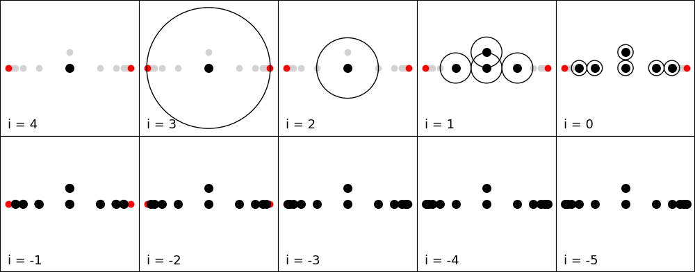
Figure 6: Example for which ICT Basic might give a relative diversity of almost 8. Each part of the figure corresponds to one layer of the cover tree. The data set $V$ (with $\mu=\eta=0.1$) is plotted as grey dots. Nodes are plotted as black dots, encircled with a ball defined by the corresponding covering radius. The optimal solution for $k=2$ with $d^{*}\approx 16$ is plotted as red dots. ICT Basic randomly selects two nodes from the first layer with at least $k$ nodes (here: fourth layer, $i=1$).

Note, for this example ICT Inherit would select a subset with higher diversity: either ${\left(0,0\right)}^{T}$ and ${\left(4,0\right)}^{T}$, or ${\left(0,0\right)}^{T}$ and ${\left(-4,0\right)}^{T}$ will be the selected nodes. Thus, $div(S^{\mathrm{ICTInherit}})=4$.

E.2 Tightness of $\alpha^{\mathrm{ICTGreedy}}$ and $\alpha^{\mathrm{ICTInherit}}$

Let the data set be defined as

$$V=\left\{v|v\in\left\{0,\pm\left(1-\mu\right),\pm\left(\frac{b}{b-1}+1-\eta\right)\right\}\;\;\cup\bigcup_{J\in[1,J_{max}]}\pm\left\{1+\sum_{j=1}^{J}{\frac{1}{b}}^{j-1}\right\}\right\},$$ (78)

where $\mu,\eta>0$ small. Note that, the value of $\mu$ must be chosen such that $i=0$ is the largest possible integer with $b^{i}<1+\mu$. Furthermore, $J_{max}$ is the smallest integer such that

$${\frac{1}{b}}^{J_{max}}\leq\eta.$$ (79)

All of the data points in $V$ lie on the line between $-\left(\frac{b}{b-1}+1-\mu\right)$ and $\left(\frac{b}{b-1}+1-\mu\right)$, where the distance between neighboring data points decreases as we move to the ends of the line. We choose the Euclidean distance as distance metric. The optimal solution $S^{*}\subseteq V$ for $k=2$ is given by

$$S^{*}=\left\{-\left(\frac{b}{b-1}+1-\eta\right),\left(\frac{b}{b-1}+1-\eta\right)\right\}$$ (80)

with a diversity of

$$d^{*}=2\left(\frac{b}{b-1}+1\right)-2\eta\;\;\approx\;\;2\left(\frac{b}{b-1}+1\right).$$ (81)

The cover tree for $V$ is built with base $b$ such that data points are incrementally added, ordered according to their absolute $x$ value. As a result, we get the following cover tree:

• $i>i_{ter}$: $C_{i}=\left\{0\right\}$

• $i_{ter}=0$: $C_{i_{ter}}=C_{i_{ter}+1}\cup\left\{-\left(1+\mu\right),1+\mu\right\}$

• $i_{ter}>i>i_{min}$: $C_{i}=C_{i+1}\cup\left\{-\left(\sum_{j=1}^{-i}{\frac{1}{b}}^{j-1}\right),\sum_{j=1}^{-i}{\frac{1}{b}}^{j-1}\right\}$

• $i_{min}$: $C_{i_{min}}=C_{i_{min}+1}\cup\left\{-\left(\frac{b}{b-1}+1-\eta\right),\frac{b}{b-1}+1-\eta\right\}$.

The data point $0$ will be the root node and each lower layer of the tree will hold the next two outer data points on the line. Any layer before level $i_{ter}$ (the termination layer) will hold only the root. The layer with $i_{min}=-\left(J_{max}+1\right)$ will hold the whole data set $V$. We will proof the cover tree properties to show that this is a valid cover tree. (1) Nesting: Obviously holds, as $C_{i+1}\subseteq C_{i}$. (2) Covering: Obviously holds for $i>i_{ter}$, because those layers only hold the root. For $i=i_{ter}=0$, the maximal distance of any point in $C_{0}$ to the root $0$ is $d(0,1+\mu)=1+\mu$. Since $i_{ter}$ is the largest possible integer $i$, such that $b^{i}<1+\mu$ (see above), it follows $b^{i_{ter}+1}\geq 1+\mu$. Let $i_{ter}>i>i_{min}$ be an arbitrary level. The nodes $-\left(1+\sum_{j=1}^{-(i+1)}{\frac{1}{b}}^{j-1}\right)$ and $1+\sum_{j=1}^{-(i+1)}{\frac{1}{b}}^{j-1}$ are the parents of the nodes $1+\sum_{j=1}^{-i}{\frac{1}{b}}^{j-1}$ and $1+\sum_{j=1}^{-i}{\frac{1}{b}}^{j-1}$. Their distance can be computed as

$$d\left(1+\sum_{j=1}^{-(i+1)}{\frac{1}{b}}^{j-1},1+\sum_{j=1}^{-i}{\frac{1}{b}}^{j-1}\right)$$ (82)

$$=\sqrt{{\left(\left(1+\sum_{j=1}^{-(i+1)}{\frac{1}{b}}^{j-1}\right)-\left(1+\sum_{j=1}^{-i}{\frac{1}{b}}^{j-1}\right)\right)}^{2}}$$ (83)

$$=\sqrt{{\left(\left(1+\sum_{j=1}^{-(i+1)}{\frac{1}{b}}^{j-1}\right)-\left(1+\sum_{j=1}^{-(i+1)}{\frac{1}{b}}^{j-1}+{\frac{1}{b}}^{-(i+1)}\right)\right)}^{2}}$$ (84)

$$={\frac{1}{b}}^{-(i+1)}$$ (85)

$$={b}^{i+1}$$ (86)

(analogously for negative data points). Therefore, the covering property holds. It also holds for level $i_{min}$, because the nodes $-\left(1+\sum_{j=1}^{J_{max}}{\frac{1}{b}}^{j-1}\right)$ and $1+\sum_{j=1}^{J_{max}}{\frac{1}{b}}^{j-1}$ are the parents of the nodes $-\left(\frac{b}{b-1}+1-\eta\right)$ and $\frac{b}{b-1}+1-\eta$. Their distance can be computed as

$$d\left(1+\sum_{j=1}^{J_{max}}{\frac{1}{b}}^{j-1},\frac{b}{b-1}+1-\eta\right)$$ (87)

$$=\sqrt{{\left(\left(\frac{b}{b-1}+1-\frac{{\frac{1}{b}}^{J_{max}-1}}{b-1}\right)-\left(\frac{b}{b-1}+1-\eta\right)\right)}^{2}}$$ (88)

$$=\sqrt{{\left(\eta-\frac{{\frac{1}{b}}^{J_{max}-1}}{b-1}\right)}^{2}}$$ (89)

$$\underset{\leq}{\eqref{eq:eta_greedy}}\sqrt{{\left({\frac{1}{b}}^{J_{max}}-\frac{{\frac{1}{b}}^{J_{max}-1}}{b-1}\right)}^{2}}$$ (90)

$$=\sqrt{{\left({\frac{1}{b}}^{J_{max}}\left(1-b\right)\left(\frac{1}{b-1}\right)\right)}^{2}}$$ (91)

$$=\sqrt{{\left(-{\frac{1}{b}}^{J_{max}}\right)}^{2}}$$ (92)

$$={\frac{1}{b}}^{J_{max}}$$ (93)

$$={\frac{1}{b}}^{-(i_{min}+1)}$$ (94)

$$=b^{i_{min}+1}$$ (95)

(analogously for the negative data points). Thus, the covering property holds for every layer of the cover tree.

(3) Separation: For every $i_{max}>i\geq i_{min}$, the closest pairwise distance we observe in layer $C_{i}$ for any node is the distance to the (self-child) of its parent. For level $i=i_{ter}=0$ the closest distance of nodes in $C_{i}$ is $1+\mu>b^{0}$, therefore, the separation property holds. Let $0>i\geq i_{min}$ be an arbitrary level. This distance to a parent was computed in Eq. (82) (or Eq. (87)) to be $b^{i+1}$, which is larger than $b^{i}$. Thus, the separation property holds for every layer of the tree.

We have seen, that the above defined cover tree is valid and fullfills the cover tree properties. The termination layer for $k=2$ is $C_{0}$. When applying ICT Inherit, we will get $S^{\mathrm{ICTInherit}}=\left\{0,1+\mu\right\}$ or $S^{\mathrm{ICTInherit}}=\left\{0,-\left(1+\mu\right)\right\}$ as a diverse subset, with

$$div(S^{\mathrm{ICTInherit}})=1+\mu\approx 1.$$ (97)

Comparing the approximated diverse subset with the optimal solution, we get

$$\underset{\mu,\eta\rightarrow 0}{\lim}\;\;\frac{d^{*}}{div(S^{\mathrm{ICTInherit}})}=\frac{2b}{b-1}+2,$$ (98)

i.e. the worst possible approximation factor. ICT Greedy can give the same solution when the root node is randomly chosen in the first iteration. Thus, we also get

$$\underset{\mu,\eta\rightarrow 0}{\lim}\;\;\frac{d^{*}}{div(S^{\mathrm{ICTGreedy}})}=\frac{2b}{b-1}+2.$$ (99)

Thus, we have shown, that no tighter approximation factor for ICT Greedy and ICT Inherit exists. The following part gives an example with $b$ set to 2.

E.2.1 Example for $b=2$

Let the data set be defined as

$$V=\left\{v|v\in\pm\left\{0,1+\mu,2,2.5,2.75,2.875,\ldots 3-\eta\right\}\right\}$$ (100)

where $\mu,\eta>0$ small. Because $\eta\neq 0$, $V$ is finite. We use Euclidean distance as distance metric. For $k=2$ the optimal solution is given by $-(3-\eta)$ and $3-\eta$ with $d^{*}\approx 6$. The cover tree is built with $b=2$ such that data points are incrementally added, ordered according to their absolute value. Figure 7 shows the first ten layer of the cover tree with $i_{max}=3$. The first layer with at least $k$ nodes is level $i=0$ (fourth layer). ICT Inherit is initialized with the root and selects one of the remaining nodes of level $0$. Thus, $S^{\mathrm{ICTInherit}}=\{0,-(1+\mu)\}$ or $S^{\mathrm{ICTInherit}}=\{0,1+\mu\}$ with $div(S^{\mathrm{ICTInherit}})\approx 1$. Thus, we get

$$\underset{\mu,\eta\rightarrow 0}{\lim}\;\;\frac{d^{*}}{div(S^{\mathrm{ICTInherit}})}=6$$ (101)

which shows the tightness of the derived approximation factor.

When the root is selected randomly as first data point of the solution, ICT Greedy can return the same solution as ICT Inherit. Thus, we also get

$$\underset{\mu,\eta\rightarrow 0}{\lim}\;\;\frac{d^{*}}{div(S^{\mathrm{ICTGreedy}})}=6.$$ (102)

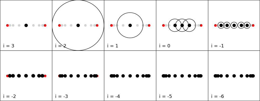
Figure 7: Example for which ICT Greedy and ICT Inherit might give a relative diversity of almost 6. Each part of the figure corresponds to one layer of the cover tree. The data set $V$ (with $\mu=\eta=0.1$) is plotted as gray dots. Nodes are plotted as black dots, encircled with a ball defined by the corresponding covering radius. The optimal solution for $k=2$ with $d^{*}\approx 6$ is plotted as red dots. ICT Inherit selects the root node and one of the two nodes from the first layer with at least $k$ nodes (here: fourth layer, $i=0$). ICT Greedy can return the same solution as ICT Inherit, when the root is selected randomly as first data point of the solution.

Appendix F Additional Figures and Tables

Figure 8 shows each layer of a cover tree built with $b=2$ on a 2D grid data example with $k=9$.

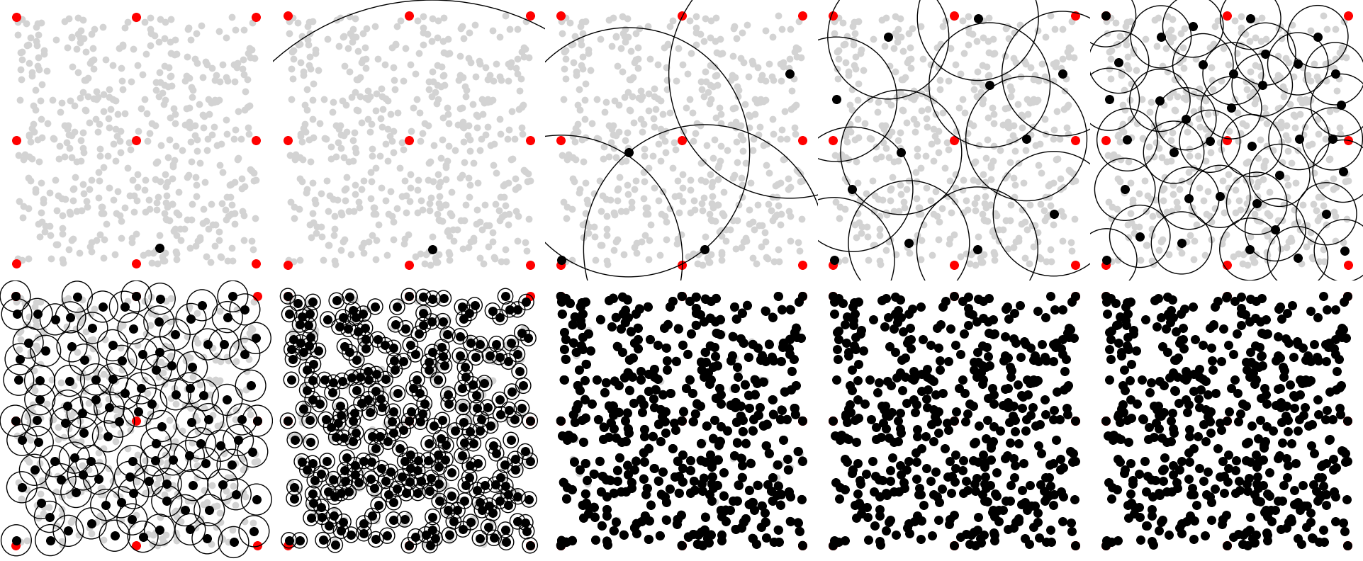
Figure 8: Example of a cover tree with $b=2$ for a two dimensional data set (grey, red). Each plot shows one level $i$ of the cover tree with all nodes (black) encircled with a ball of radius $2^{i}$. The red dots correspond to the optimal diverse solution with $k=9$.

Table 1 summarizes information for the artificial and real data in our experiments. For the cover tree we used the implementation provided in [7].

Table 1: Summary of conducted experiments.

	Experiment	Dimension	Sample Size	Diverse Set Size k	Distance Metric
Artificial	Grid 2D	$2$	$\{500,1000,5000\}$	$\{4,9,25\}$	Euclidean
	Grid 5D	$5$	$5000$	$\{32,243,1024\}$	Euclidean
Real	Cities	$2$	$10975$	$[2,100]$	Euclidean
	Faces	$624$	$3840$	$[2,100]$	Cosine
	MNIST	$784$	$70000$	$[2,100]$	Cosine

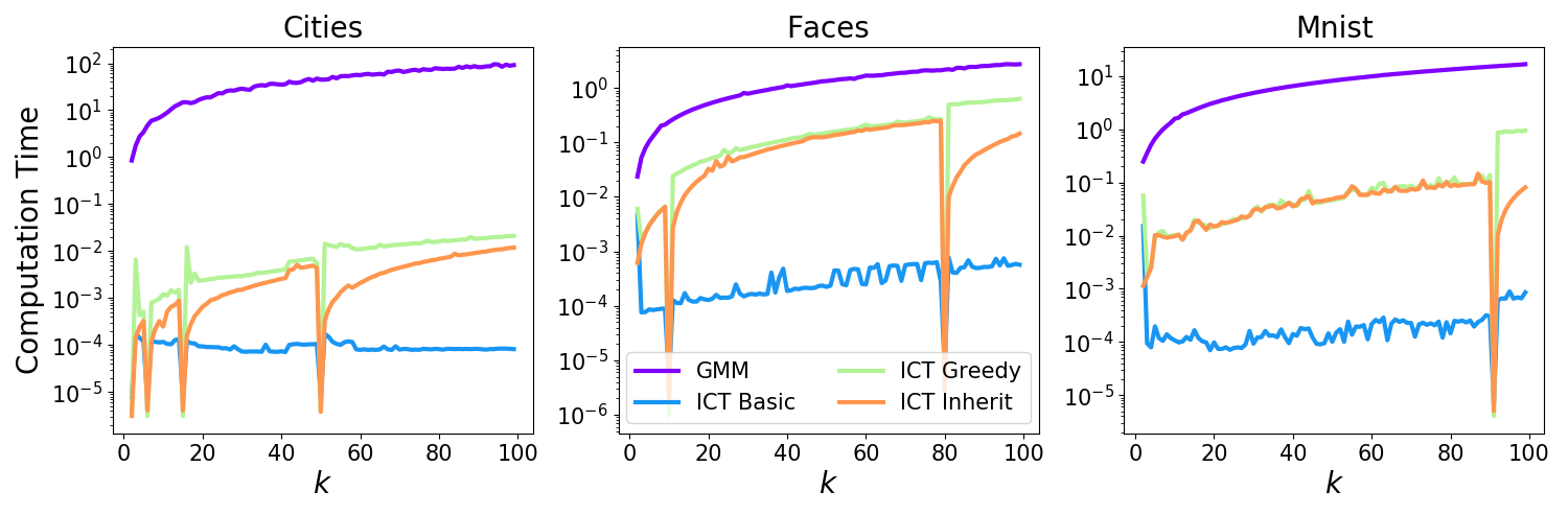
Figure 9: Computation time in ms on the Cities, Faces and MNIST data sets. All experiments were conducted on a Intel(R) Xeon(R) CPU E5-2640 v4 with 2.40GHz.

Figure 9 shows the computation time of selecting the diverse subsets for the different approaches. One can clearly see the efficiency of the cover-tree approaches. Compared to GMM, ICT Basic, ICT Greedy and ICT Inherit have fast computation time even for large $k$. The computation time of the cover tree approaches shows a step function behavior. Again, this can be explained by the layer-wise structure of the cover tree. When the termination layer holds exactly $k$ nodes, no selection must be made. We can also see the difference in the complexity of ICT Greedy and ICT Inherit. When the layer before the termination layer holds almost $k$ nodes, i.e. $|C_{i+1}|\approx|C_{i}|$, ICT Inherit only has to select few nodes.

Appendix G Examples of diverse images generated by PPGN

Figs. 10–17 show the $k=5$ randomly chosen images (left) from the MCMC sequence of PPGN conditioned on several ImageNet classes, and the corresponding diverse sets (right) chosen by ICT Inherit, after 20 (bottom), 100 (middle), and 200 (top) MCMC steps. We can see that ICT Inherit chose more diverse images in shape (e.g., Volcano (Fig. 5), Greenhouses, Spiders), composition (e.g., Sheep, Clocks), and color (e.g., Train).

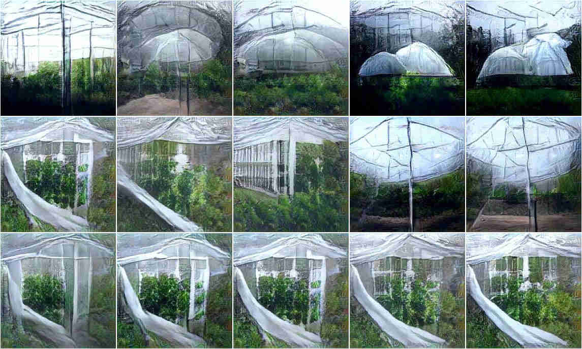
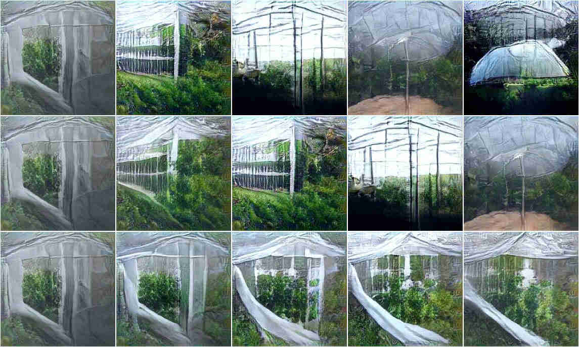
Figure 10: $k=5$ randomly chosen images (left) from the MCMC sequence of PPGN for Greenhouse class, and the corresponding diverse sets (right) chosen by ICT Inherit, after 20 (bottom), 100 (middle), and 200 (top) MCMC steps.

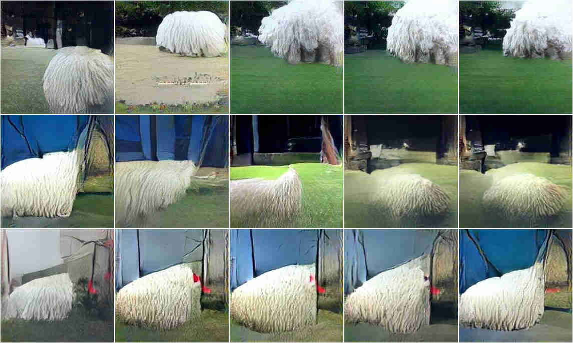
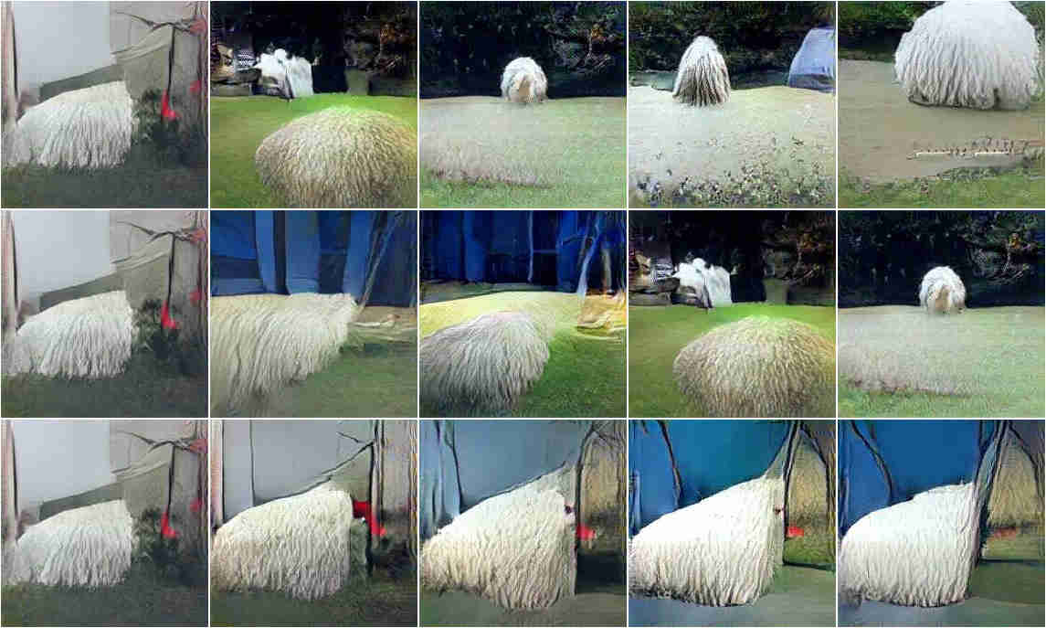
Figure 11: $k=5$ randomly chosen images (left) from the MCMC sequence of PPGN for Sheep class, and the corresponding diverse sets (right) chosen by ICT Inherit, after 20 (bottom), 100 (middle), and 200 (top) MCMC steps.

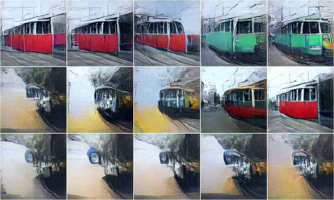
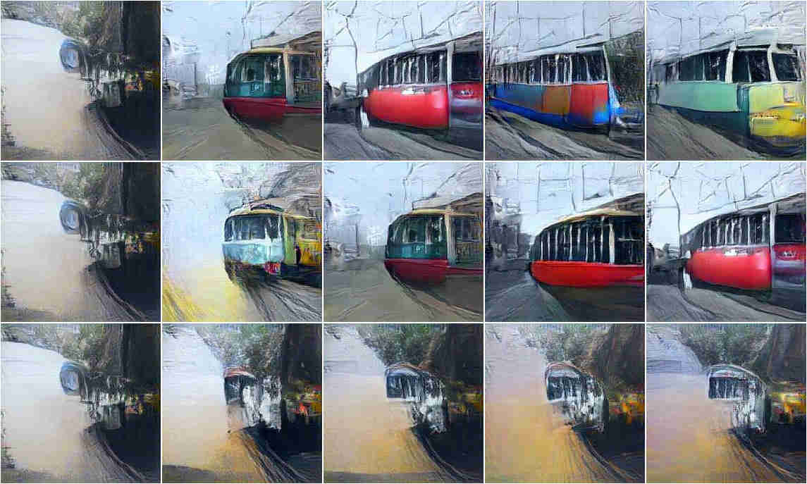
Figure 12: $k=5$ randomly chosen images (left) from the MCMC sequence of PPGN for Train class, and the corresponding diverse sets (right) chosen by ICT Inherit, after 20 (bottom), 100 (middle), and 200 (top) MCMC steps.

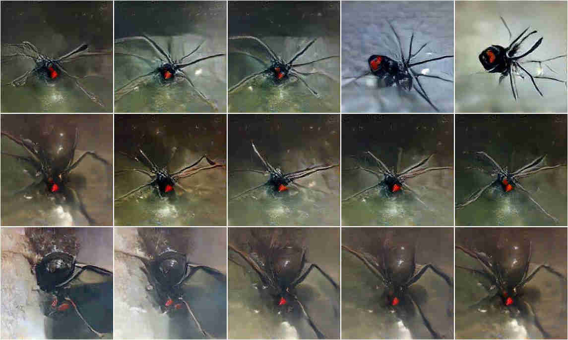
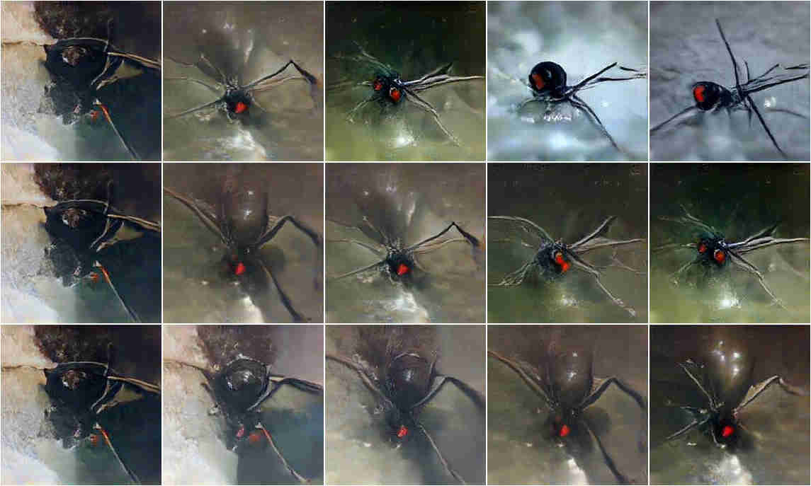
Figure 13: $k=5$ randomly chosen images (left) from the MCMC sequence of PPGN for Spider class, and the corresponding diverse sets (right) chosen by ICT Inherit, after 20 (bottom), 100 (middle), and 200 (top) MCMC steps.

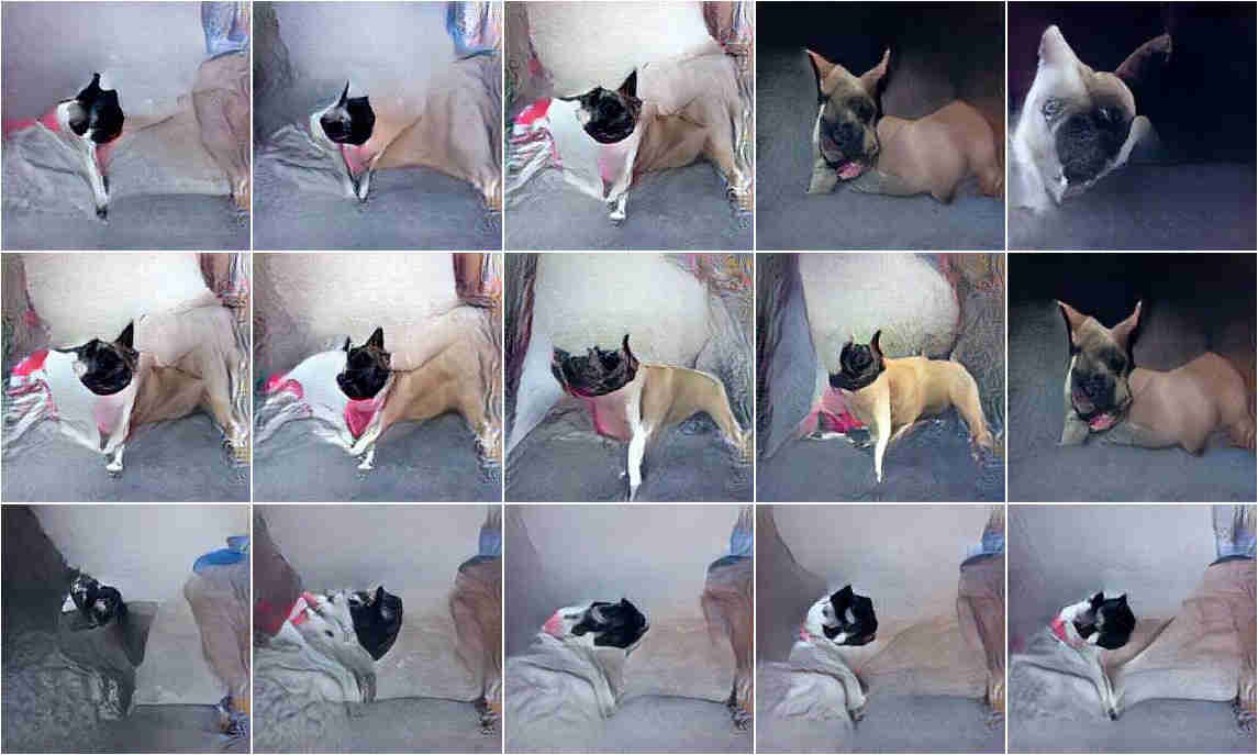
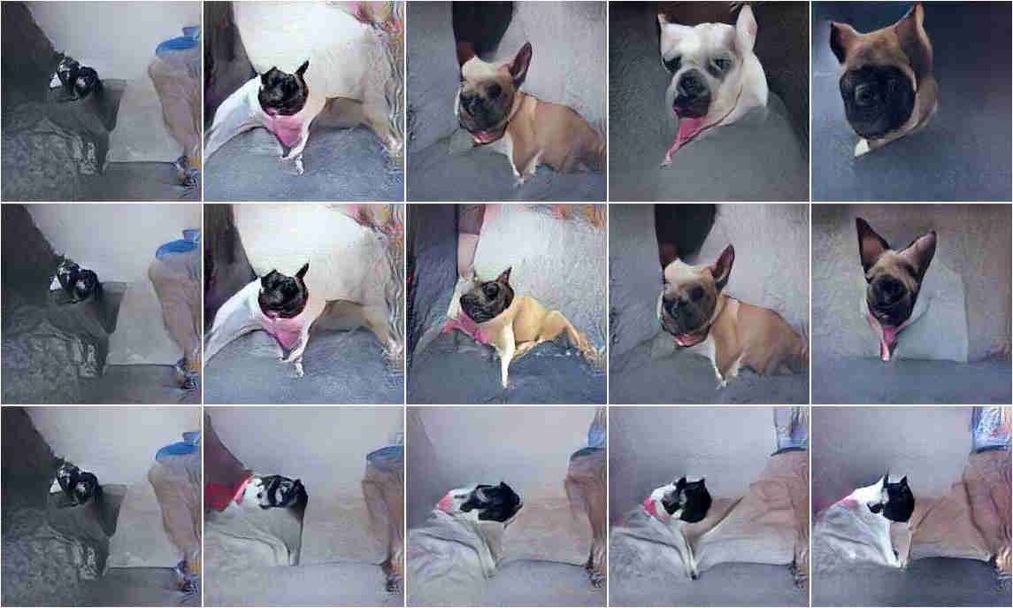
Figure 14: $k=5$ randomly chosen images (left) from the MCMC sequence of PPGN for Dog class, and the corresponding diverse sets (right) chosen by ICT Inherit, after 20 (bottom), 100 (middle), and 200 (top) MCMC steps.

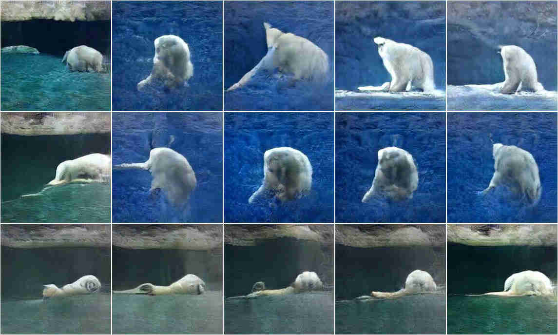
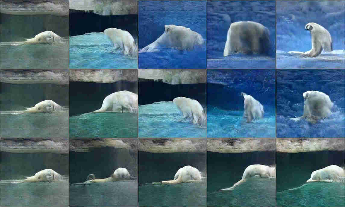
Figure 15: $k=5$ randomly chosen images (left) from the MCMC sequence of PPGN for Polar Bear class, and the corresponding diverse sets (right) chosen by ICT Inherit, after 20 (bottom), 100 (middle), and 200 (top) MCMC steps.

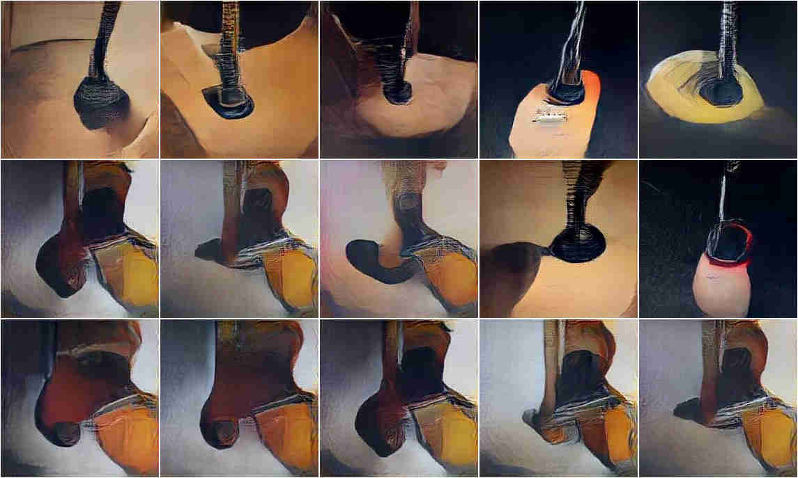
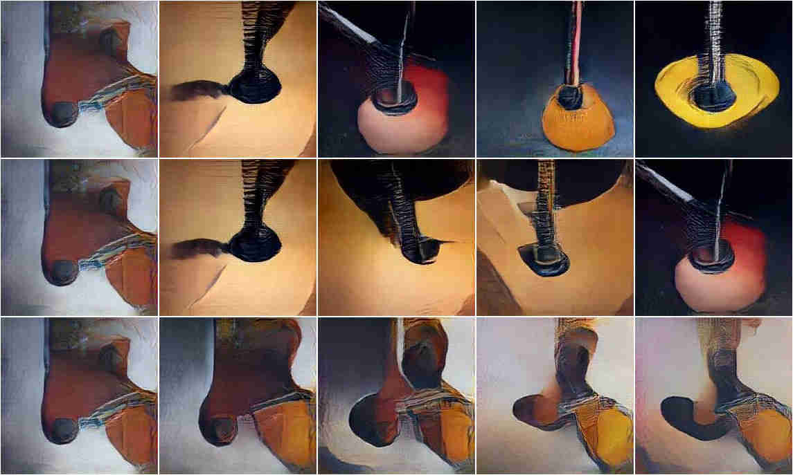
Figure 16: $k=5$ randomly chosen images (left) from the MCMC sequence of PPGN for Guitar class, and the corresponding diverse sets (right) chosen by ICT Inherit, after 20 (bottom), 100 (middle), and 200 (top) MCMC steps.

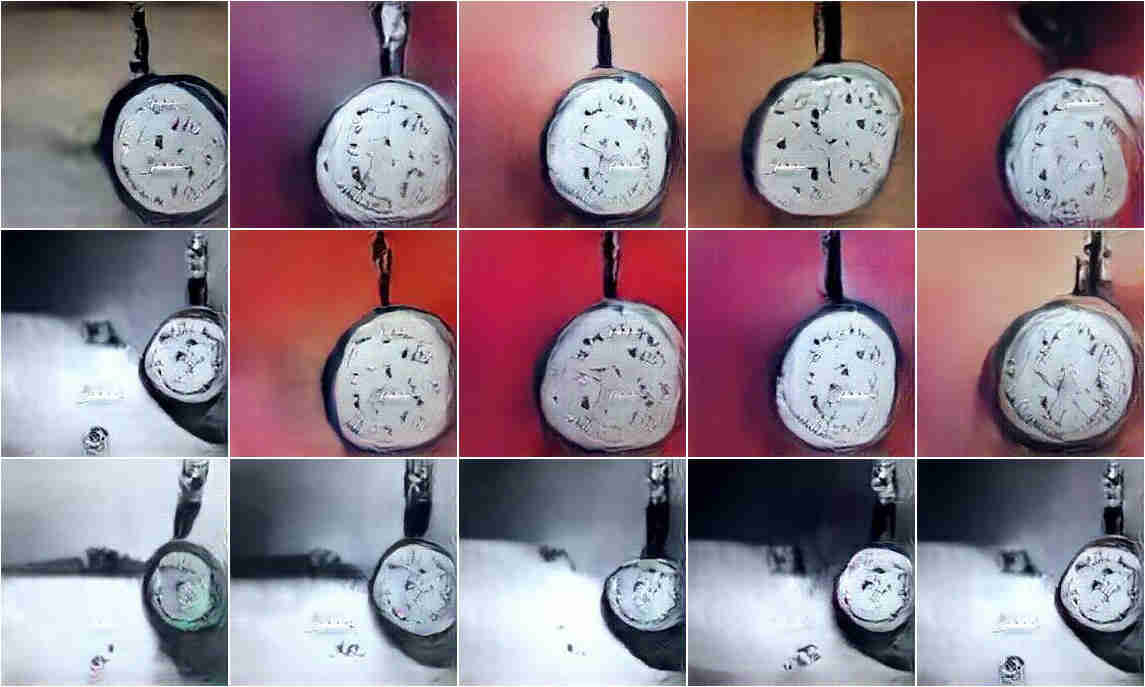
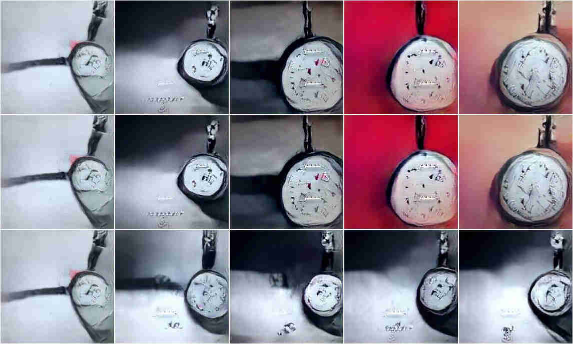
Figure 17: $k=5$ randomly chosen images (left) from the MCMC sequence of PPGN for Clock class, and the corresponding diverse sets (right) chosen by ICT Inherit, after 20 (bottom), 100 (middle), and 200 (top) MCMC steps.

References

- [1] Sofiane Abbar, Sihem Amer-Yahia, Piotr Indyk, Sepideh Mahabadi, and Kasturi R Varadarajan. Diverse near neighbor problem. In Proceedings of the twenty-ninth annual symposium on Computational geometry, pages 207–214. ACM, 2013.
- [2] The UCI KDD Archive. CMU faces images. http://kdd.ics.uci.edu/databases/faces/faces.html. Accessed on 2018-05-18.
- [3] Alina Beygelzimer, Sham Kakade, and John Langford. Cover trees for nearest neighbor. In Proc. of ICML, pages 97–104, 2006.
- [4] Alina Beygelzimer, Sham Kakade, and John Langford. Cover trees for nearest neighbor. In Proceedings of the 23rd international conference on Machine learning, pages 97–104. ACM, 2006.
- [5] Center For International Earth Science Information Network-CIESIN-Columbia University. Gridded population of the world: Basic demographic characteristics. https://doi.org/10.7927/H45H7D7F. Accessed on 2016-12-13.
- [6] E. Demidova, P. Fankhauser, X. Zhou, and W. Nejdl. DivQ: Diversification for keyword search over structured databases. In Proc. of SIGIR, pages 331–338, 2010.
- [7] Marina Drosou and Evaggelia Pitoura. Poikilo: A tool for evaluating the results of diversification models and algorithms. Proceedings of the VLDB Endowment, 6(12):1246–1249, 2013.
- [8] Marina Drosou and Evaggelia Pitoura. Diverse set selection over dynamic data. IEEE Transactions on Knowledge and Data Engineering, 26(5):1102–1116, 2014.
- [9] E. Erkut. The discrete -dispersion problem. European Journal of Operational Research, 1(1), 1990.
- [10] E. Erkut, Y. Ulkusal, and O Yenicerioglu. A comparison of -dispersion heuristics. Computers and Operations Research, 21(10), 1995.
- [11] S. Gollapudi and A. Sharma. An axiomatic approach for result diversification. In Proc. of WWW, pages 381–390, 2009.
- [12] M. Izbicki and C. R. Shelton. Fast cover trees. In Proc. of ICML, 2015.
- [13] Matevž Kunaver and Tomaž Požrl. Diversity in recommender systems–a survey. Knowledge-Based Systems, 123:154–162, 2017.
- [14] Yann LeCun and Corinna Cortes. MNIST handwritten digit database. http://yann.lecun.com/exdb/mnist/, 2010.
- [15] Z. Liu, P. Sun, and Y. Chen. Structured search result differentiation. In Proc. of VLDB, 2009.
- [16] E. Minack, W. Siberski, and W. Nejdl. Incremental diversification for very large sets: A streaming-based approach. In Proc. of SIGIR, 2011.
- [17] A. Nguyen, J. Clune, Y. Bengio, A. Dosovitskiy, and J. Yosinski. Plug & play generative networks: Conditional iterative generation of images in latent space. In 2017 IEEE Conference on Computer Vision and Pattern Recognition (CVPR), pages 3510–3520, 2017.
- [18] SS Ravi, Daniel J Rosenkrantz, and Giri Kumar Tayi. Facility dispersion problems: Heuristics and special cases. In Workshop on Algorithms and Data Structures, pages 355–366. Springer, 1991.
- [19] E. Vee, U. Srivastava, J. Shanmugasundaram, P. Bhat, and S. A. Yahia. Efficient computation of diverse query results. In Proc. of ICDE, pages 228–236, 2008.
- [20] M. R. Vieira, H. L. Razente, M. C. N. Barioni, M. Hadjieleftheriou, D. Srivastava, C. T. Jr., and V. J. Tsotras. On query result diversification. In Proc. of ICDE, 2011.
- [21] David P Williamson and David B Shmoys. The design of approximation algorithms. Cambridge university press, 2011.
- [22] C. Yu, L. V. Lakshmanan, and S. Amer-Yahia. Recommendation diversification using explanations. In Proc. of ICDE, 2009.
- [23] M. Zhang and N. Hurley. Avoiding monotony: Improving the diversity of recommendation lists. In Proc. of RecSys, 2008.
- [24] C.-N. Ziegler, S. M. McNee, J. A. Konstan, and G. Lausen. Improving recommendation lists through topic diversification. In Proc. of WWW, pages 381–390, 2005.