Stochastic WaveNet: A Generative Latent Variable Model for Sequential Data

Abstract

How to model distribution of sequential data, including but not limited to speech and human motions, is an important ongoing research problem. It has been demonstrated that model capacity can be significantly enhanced by introducing stochastic latent variables in the hidden states of recurrent neural networks. Simultaneously, WaveNet, equipped with dilated convolutions, achieves astonishing empirical performance in natural speech generation task. In this paper, we combine the ideas from both stochastic latent variables and dilated convolutions, and propose a new architecture to model sequential data, termed as Stochastic WaveNet, where stochastic latent variables are injected into the WaveNet structure. We argue that Stochastic WaveNet enjoys powerful distribution modeling capacity and the advantage of parallel training from dilated convolutions. In order to efficiently infer the posterior distribution of the latent variables, a novel inference network structure is designed based on the characteristics of WaveNet architecture. State-of-the-art performances on benchmark datasets are obtained by Stochastic WaveNet on natural speech modeling and high quality human handwriting samples can be generated as well.

1 Introduction

Learning to capture complex distribution of sequential data is an important machine learning problem and has been extensively studied in recent years. The autoregressive neural network models, including Recurrent Neural Network (Hochreiter and Schmidhuber,, 1997; Chung et al.,, 2014), PixelCNN (Oord et al.,, 2016) and WaveNet (Van Den Oord et al.,, 2016), have shown strong empirical performance in modeling natural language, images and human speeches. All these methods are aimed at learning a deterministic mapping from the data input to the output. Recently, evidence has been found (Fabius and van Amersfoort,, 2014; Gan et al.,, 2015; Gu et al.,, 2015; Goyal et al.,, 2017; Shabanian et al.,, 2017) that probabilistic modeling with neural networks can benefit from uncertainty introduced to their hidden states, namely including stochastic latent variables in the network architecture. Without such uncertainty in the hidden states, RNN, PixelCNN and WaveNet would parameterize the randomness only in the final layer by shaping a output distribution from the specific distribution family. Hence the output distribution (which is often assumed to be Gaussian for continuous data) would be unimodal or the mixture of unimodals given the input data, which may be insufficient to capture the complex true data distribution and to describe the complex correlations among different output dimensions (Boulanger-Lewandowski et al.,, 2012). Even for the non-parametrized discrete output distribution modeled by the softmax function, a phenomenon referred to as softmax bottleneck (Yang et al., 2017a, ) still limits the family of output distributions. By injecting the stochastic latent variables into the hidden states and transforming their uncertainty to outputs by non-linear layers, the stochastic neural network is equipped with the ability to model the data with a much richer family of distributions.

Motivated by this, numerous variants of RNN-based stochastic neural network have been proposed. STORN (Bayer and Osendorfer,, 2014) is the first to integrate stochastic latent variables into RNN’s hidden states. In VRNN (Chung et al.,, 2015), the prior of stochastic latent variables is assumed to be a function over historical data and stochastic latent variables, which allows them to capture temporal dependencies. SRNN (Fraccaro et al.,, 2016) and Z-forcing (Goyal et al.,, 2017) offer more powerful versions with augmented inference networks which better capture the correlation between the stochastic latent variables and the whole observed sequence. By introducing stochasticity to the hidden states, these RNN-based models achieved significant improvements over vanilla RNN models on log-likelihood evaluations on multiple benchmark datasets from various domains (Goyal et al.,, 2017; Shabanian et al.,, 2017).

In parallel with RNN, WaveNet (Van Den Oord et al.,, 2016) provides another powerful way of modeling sequential data with dilated convolutions, especially in the natural speech generation task. While RNN-based models must be trained in a sequential manner, training a WaveNet can be easily parallelized. Furthermore, the parallel WaveNet proposed in (Oord et al.,, 2017) is able to generate new sequences in parallel. WaveNet, or dilated convolutions, has also been adopted as the encoder or decoder in the VAE framework and produces reasonable results in the text (Semeniuta et al.,, 2017; Yang et al., 2017b, ) and music (Engel et al.,, 2017) generation task.

In light of the advantage of introducing stochastic latent variables to RNN-based models, it is natural to raise a problem whether this benefit carries to WaveNet-based models. To this end, in this paper we propose Stochastic WaveNet, which associates stochastic latent variables with every hidden states in the WaveNet architecture. Compared with the vanilla WaveNet, Stochastic WaveNet is able to capture a richer family of data distributions via the added stochastic latent variables. It also inherits the ease of parallel training with dilated convolutions from the WaveNet architecture. Because of the added stochastic latent variables, an inference network is also designed and trained jointly with Stochastic WaveNet to maximize the data log-likelihood. We believe that after model training, the multi-layer structure of latent variables leads them to reflect both hierarchical and sequential structures of the data. This hypothesis is validated empirically by controlling the number of layers of stochastic latent variables.

The rest of this paper is organized as follows: we briefly review the background in Section 2. The proposed model and optimization algorithm are introduced in Section 3. We evaluate and analyze the proposed model on multiple benchmark datasets in Section 4. Finally, the summary of this paper is included in Section 5.

2 Preliminary

2.1 Notation

We first define the mathematical symbols used in the rest of this paper. We denote a set of vectors by a bold symbol, such as ${\boldsymbol{x}}$, which may utilize one or two dimension subscripts as index, such as ${\boldsymbol{x}}_{i}$ or ${\boldsymbol{x}}_{i,j}$. $f(\cdot)$ represents the general function that transforms an input vector to a output vector. And $f_{\theta}(\cdot)$ is a neural network function parametrized by $\theta$. For a sequential data sample ${\boldsymbol{x}}$, $T$ represents its length.

2.2 Autoregressive Neural Network

Autoregressive network model is designed to model the joint distribution of the high-dimensional data with sequential structure, by factorizing the joint distribution of a data sample as

$$p({\boldsymbol{x}})=\prod_{t=1}^{T}p_{\theta}(x_{t}|x_{<t})$$ (1)

where ${\boldsymbol{x}}=\{x_{1},x_{2},\cdots x_{T}\},x_{t}\in R^{d}$, $t$ indexes the temporal time stamps, and $\theta$ represents the model parameters. Then the autoregressive model can compute the likelihood of a sample and generate a new data sample in a sequential manner.

In order to capture richer stochasticities of the sequential generation process, stochastic latent variables for each time stamp have been introduced, referred to as stochastic neural network (Chung et al.,, 2015; Fraccaro et al.,, 2016; Goyal et al.,, 2017). Then the joint distribution of the data together with the latent variables is factorized as,

$$p({\boldsymbol{x}},{\boldsymbol{z}}) =\prod_{t=1}^{T}p_{\theta}(x_{t},z_{t}|x_{<t},z_{<t})$$ (2)

$$=\prod_{t=1}^{T}p_{\theta}(x_{t}|x_{<t},z_{\leq t})p_{\theta}(z_{t}|x_{<t},z_{<t})$$

where ${\boldsymbol{z}}=\{z_{1},z_{2},\cdots z_{T}\},z_{t}\in R^{d^{\prime}}$ has the same sequence length as the data sample, $d^{\prime}$ is its dimension for one time stamp. ${\boldsymbol{z}}$ is also generated sequentially, namely the prior of $z_{t}$ is conditional probability given $x_{<t}$ and $z_{<t}$.

2.3 WaveNet

WaveNet (Van Den Oord et al.,, 2016) is a convolutional autoregressive neural network which adopts dilated causal convolutions (Yu and Koltun,, 2015) to extract the sequential dependency in the data distribution. Different from recurrent neural network, dilated convolution layers can be computed in parallel during the training process, which makes WaveNet much faster than RNN in modeling sequential data. A typical WaveNet structure is visualized in Figure 1. Beside the computation advantage, WaveNet has shown the start-of-the-art result in speech generation task (Oord et al.,, 2017).

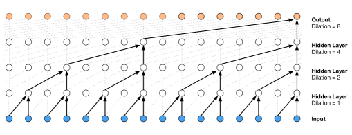
Figure 1: Visualization of a WaveNet structure from (Van Den Oord et al.,, 2016)

3 Stochastic WaveNet

In this section, we introduce a sequential generative model (Stochastic WaveNet), which imposes stochastic latent variables with the multi-layer dilated convolution structure. We firstly introduce the generation process of Stochastic WaveNet, and then describe the variational inference method.

3.1 Generative Model

Similar as stochastic recurrent neural networks, we inject the stochastic latent variable in each WaveNet hidden node in the generation process, which is illustrated in Figure 2(a). More specifically, for a sequential data sample ${\boldsymbol{x}}$ with length $T$, we introduce a set of stochastic latent variables ${\boldsymbol{z}}=\{z_{t,l}|1\leq t\leq T,1\leq l\leq L\},z_{t,l}\in{\mathbb{R}}^{d^{\prime}}$, where $L$ is the number of the layers of WaveNet architecture. Then the generation process can be described as,

$$p({\boldsymbol{x}},{\boldsymbol{z}}) =\prod_{t=1}^{T}p_{\theta}(x_{t},z_{t,1:L}|x_{<t},z_{<t,1:L})$$ (3)

$$=\prod_{t=1}^{T}[p_{\theta}(x_{t}|z_{\leq t,1:L},x_{<t})$$

$$\qquad\quad\prod_{l=1}^{L}p_{\theta}(z_{t,l}|z_{t,<l},x_{<t},z_{<t,1:L})]$$

The generation process can be interpreted as this. At each time stamp $t$, we sample the stochastic latent variables $z_{t,l}$ from a prior distribution which are conditioned on the lower level latent variables and historical records including the data samples $x_{<t}$ and latent variables $z_{<t}$. Then we sample the new data sample $x_{t}$ according to all sampled latent variables and historical records. Through this process, new sequential data samples are generated in a recursive way.

In Stochastic WaveNet, the prior distribution $p_{\theta}(z_{t,l}|x_{<t},z_{t,<l},z_{<t,1:L})={\mathcal{N}}(z_{t,l};\mu_{t,l},v_{t,l})$ is defined as a Gaussian distribution with the diagonal covariance matrix. The sequential and hierarchical dependency among the latent variables are modeled by the WaveNet architecture. In order to summarize all historical information, we introduce two stochastic hidden variables ${\boldsymbol{h}}$ and ${\boldsymbol{d}}$, which are calculated as,

$$h_{t,l} =f_{\theta_{1}}(d_{t-2^{l},l-1},d_{t,l-1})$$ (4)

$$d_{t,l} =f_{\theta_{2}}(h_{t,l},z_{t,l})$$

Where $f_{\theta_{1}}$ mimics the design of the dilated convolution in WaveNet, and $f_{\theta_{2}}$ is a fully connected layer to summarize the hidden states and the sampled latent variable. Different from the vanilla WaveNet, the hidden states ${\boldsymbol{h}}$ are stochastic because of the random samples ${\boldsymbol{z}}$. We parameterize the mean and variance of the prior distributions by the hidden representations ${\boldsymbol{h}}$, which is $\mu_{t,l}=f_{\theta_{3}}(h_{t,l})$ and $\log~{}v_{t,l}=f_{\theta_{4}}(h_{t,l})$. Similarly, we parameterize the emission probability $p_{\theta}(x_{t}|x_{<t},z_{t,1:L},z_{<t,1:L})$ as a neural network function over the hidden representations.

3.2 Variational Inference for Stochastic WaveNet

Instead of directly maximizing log-likelihood for a sequential sample ${\boldsymbol{x}}$, we optimize its variational evidence lower bound (ELBO) (Jordan et al.,, 1999). Exact posterior inference of the stochastic variables ${\boldsymbol{z}}$ of Stochastic WaveNet is intractable. Hence, we describe a variational inference method for Stochastic WaveNet by utilizing the reparameterization trick introduced in (Kingma and Welling,, 2013). Firstly, we write the ELBO as,

$$\log~{}p({\boldsymbol{x}}) \geq\int q_{\phi}({\boldsymbol{z}}|{\boldsymbol{x}})\log\frac{p_{\theta}({\boldsymbol{x}},{\boldsymbol{z}})}{q_{\phi}({\boldsymbol{z}}|{\boldsymbol{x}})}dz$$ (5)

$$={\mathbb{E}}_{q_{\phi}({\boldsymbol{z}}|{\boldsymbol{x}})}[\sum_{t=1}^{T}\log~{}p_{\theta}(x_{t}|z_{\leq t,1:L},x_{<t})]$$

$$\qquad-D_{KL}(q_{\phi}({\boldsymbol{z}}|{\boldsymbol{x}})||p_{\theta}({\boldsymbol{z}}|{\boldsymbol{x}}))$$

$$={\mathcal{L}}(x)$$

$$where ~{}~{}p_{\theta}({\boldsymbol{z}}|{\boldsymbol{x}})=\prod_{t=1}^{T}\prod_{l=1}^{L}p_{\theta}(z_{t,l}|z_{t,<l},x_{<t},z_{<t,1:L})$$

We can derive the second equation by taking Eq. 3 into the first equation, and ${\mathcal{L}}(x)$ denotes the loss function for the sample ${\boldsymbol{x}}$. Here another problem needs to be addressed is how to define the posterior distribution $q_{\phi}({\boldsymbol{z}}|{\boldsymbol{x}})$. In order to maximize the ELBO, we factorize the posterior as,

$$q_{\phi}({\boldsymbol{z}}|{\boldsymbol{x}})=\prod_{t=1}^{T}\prod_{l=1}^{L}q_{\phi}(z_{t,l}|{\boldsymbol{x}},z_{t,<l},z_{<t,1:L})$$ (6)

Here the posterior distribution for $z_{t,l}$ is conditioned on the stochastic latent variables sampled before it and the entire observed data ${\boldsymbol{x}}$. By utilizing the future data $x_{\geq t}$, we can better maximize the first term in ${\mathcal{L}}(x)$, the reconstruction loss term. In opposite, the prior distribution of $z_{t,l}$ is only conditioned on $x_{<t}$, so encoding $x_{\geq t}$ information may increase the degree of distribution mismatch between the prior and posterior distribution, namely enlarging the KL term in loss function.

Exploring the dependency structure in WaveNet. However, by analyzing the dependency among the outputs and hidden states of WaveNet, we would find that the stochastic latent variables at time stamp t, $z_{t,1:L}$ would not influence whole posterior outputs. So the inference network would only require partial posterior outputs to maximize the reconstruction loss term in the loss function. Denote the set of outputs that would be influenced by $z_{l,t}$ as $s(l,t)$. The posterior distribution can be modified as,

$$q_{\phi}({\boldsymbol{z}}|{\boldsymbol{x}})=\prod_{t=1}^{T}\prod_{l=1}^{L}q_{\phi}(z_{t,l}|x_{<t},x_{s(l,t)},z_{t,<l},z_{<t,1:L})$$ (7)

The modified posterior distribution removes unnecessary conditional variables, which makes the optimization more efficient. To summarize the information from posterior outputs $x_{s(l,t)}$, we design a reversed WaveNet architecture to compute the hidden feature ${\boldsymbol{b}}$, illustrated in Figure 2(b), and $b_{t,l}$ is formulated as,

$$b_{t,l}=f(x_{s(t,l)})=f_{\phi_{1}}(b_{t,l+1},b_{t+2^{l+1},l+1})$$ (8)

where we define that $b_{t,L}=f_{\phi_{2}}(x_{t},x_{t+2^{L+1}})$, and $f_{\phi_{1}}$ and $f_{\phi_{2}}$ is the dilated convolution layer, whose structure is a reverse version of $f_{\theta_{1}}$ in Eq.3. Finally, we inference the posterior distribution $q_{\phi}(z_{t,l}|{\boldsymbol{x}},z_{t,<l},z_{<t,1:L})={\mathcal{N}}(z_{t,l};\mu^{\prime}_{t,l},v^{\prime}_{t,l})$ by ${\boldsymbol{b}}$ and ${\boldsymbol{h}}$, which is $\mu^{\prime}_{t,l}=f_{\phi_{3}}(h_{t,l},b_{t,l})$ and $\log~{}v^{\prime}_{t,l}=f_{\phi_{4}}(h_{t,l},b_{t,l})$. Here, we reuse the stochastic hidden states ${\boldsymbol{h}}$ in the generative model in order to compress the number of the model parameters.

KL Annealing Trick. It is well known that the deep neural networks with multi-layers stochastic latent variables is difficult to train, of which one important reason is that the KL term in the loss function limited the capacity of the stochastic latent variable to compress the data information in early stages of training. The KL Annealing is a common trick to alleviate this issue. The objective function is redefined as,

$${\mathcal{L}}_{\lambda}({\boldsymbol{x}}) ={\mathbb{E}}_{q_{\phi}({\boldsymbol{z}}|{\boldsymbol{x}})}[\sum_{t=1}^{T}\log~{}p_{\theta}({\boldsymbol{x}}|{\boldsymbol{z}})]$$ (9)

$$\qquad-\lambda D_{KL}(q_{\phi}({\boldsymbol{z}}|{\boldsymbol{x}})||p_{\theta}({\boldsymbol{z}}|{\boldsymbol{x}}))$$

During the training process, the $\lambda$ is annealed from 0 to 1. In previous works, researchers usually adopt the linear annealing strategy (Fraccaro et al.,, 2016; Goyal et al.,, 2017). In our experiment, we find that it still increases $\lambda$ too fast for Stochastic WaveNet. We propose to use cosine annealing strategy alternatively, namely the $\lambda$ is following the function $\lambda_{\alpha}=1-cos(\alpha)$, where $\alpha$ scans from $0$ to $\frac{\pi}{2}$.

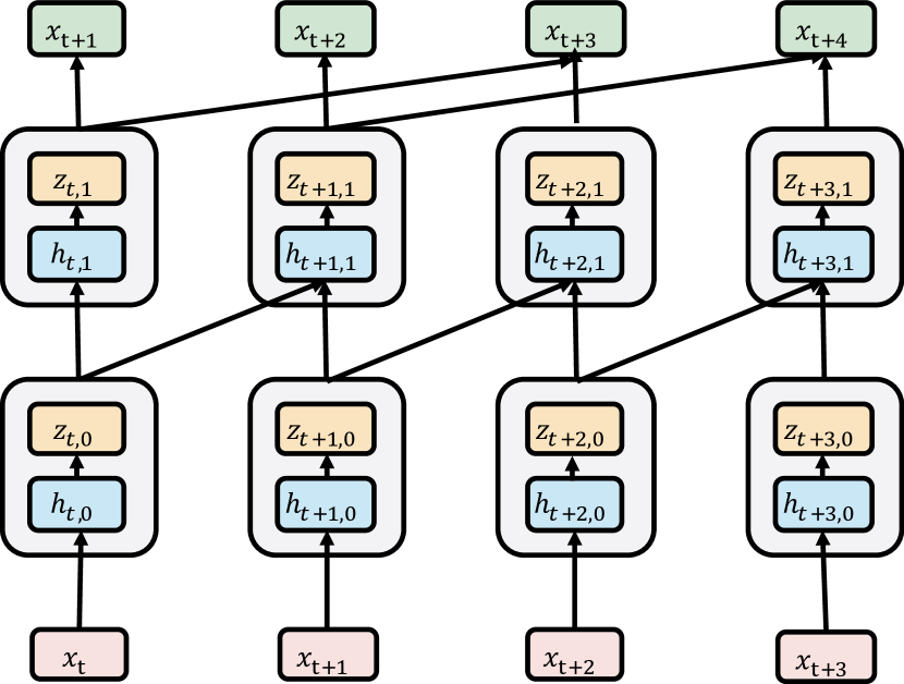
(a) Generative Model

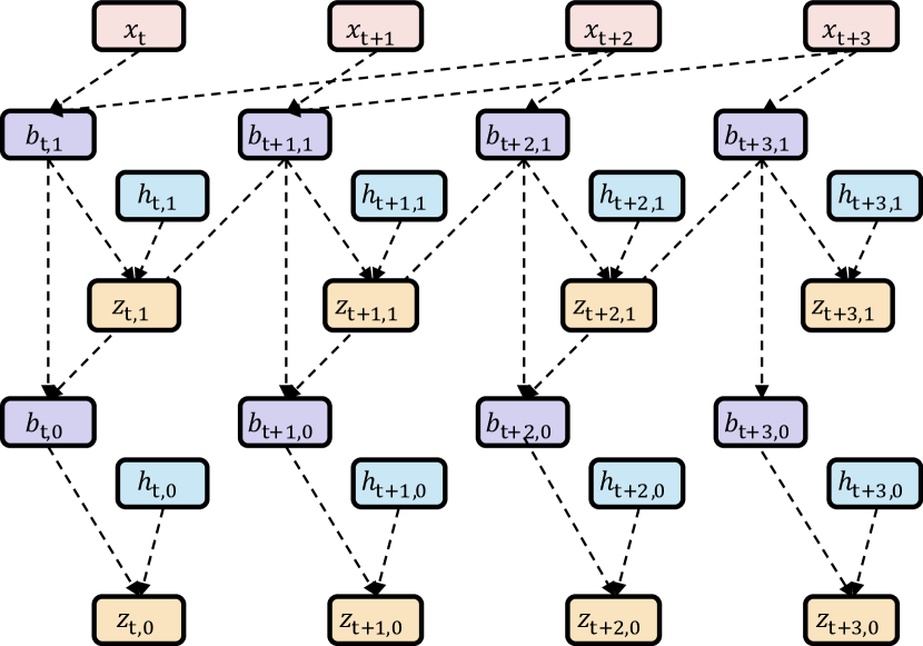
(b) Inference Model

Figure 2: This figure illustrates a toy sample of Stochastic WaveNet, which has two layers. The left one is the generative model, and the right one is the inference model. Both the solid line and dash line represent the neural network functions. The ${\boldsymbol{h}}$ in the right figure is identical to the one in the left. The ${\boldsymbol{z}}$ in the generative model are sampled from prior distributions, and the ones in the inference model are from posterior.

4 Experiment

In this section, we evaluate the proposed Stochastic WaveNet on several benchmark datasets from various domains, including natural speech, human handwriting and human motion modeling tasks. We show that Stochastic WaveNet, or SWaveNet in short, achieves state-of-the-art results, and visualizes the generated samples for the human handwriting domain. The experiment codes are publicly accessible.

Baselines. The following sequential generative models proposed in recent years are treated as the baseline methods:

• RNN: The original recurrent neural network with the LSTM cell.

• VRNN: The generative model with the recurrent structure proposed in (Chung et al.,, 2015). It firstly formulates the prior distribution of $z_{t}$ as a conditional probability given historical data $x_{<t}$ and latent variables $z_{<t}$.

• SRNN: Proposed in (Fraccaro et al.,, 2016), and it augments the inference network by a backward RNN to better optimize the ELBO.

• Z-forcing: Proposed in (Goyal et al.,, 2017), whose architecture is similar to SRNN, and it eases the training of the stochastic latent variables by adding auxiliary cost which forces model to use stochastic latent variables $z$ to reconstruct the future data $x_{>t}$.

• WaveNet: Proposed in (Van Den Oord et al.,, 2016) and produce state-of-the-art result in the speech generation task.

We evaluate different models by comparing the log-likelihood on the test set (RNN, WaveNet) or its lower bound (VRNN, SRNN, Z-forcing and our method). For fair comparison, a multivariate Gaussian distribution with the diagonal covariance matrix is used as the output distribution for each time stamp in all experiments. The Adam optimizer (Kingma and Ba,, 2014) is used for all models, and the learning rate is scheduled by the cosine annealing. Following the experiment setting in (Fraccaro et al.,, 2016), we use 1 sample to approximate the variational evidence lower bound to reduce the computation cost.

4.1 Natural Speech Modeling

In the natural speech modeling task, we train the model to fit the log-likelihood function of the raw audio signals, following the experiment setting in (Fraccaro et al.,, 2016; Goyal et al.,, 2017). The raw signals, which correspond to the real-valued amplitudes, are represented as a sequence of 200-dimensional frames. Each frame is 200 consecutive samples. The preprocessing and dataset segmentation are identical to (Fraccaro et al.,, 2016; Goyal et al.,, 2017). We evaluate the proposed model in the following benchmark datasets:

• Blizzard (Prahallad et al.,, 2013): The Blizzard Challenge 2013, which is a text-to-speech dataset containing 300 hours of English from a single female speaker.

• TIMIT : TIMIT raw audio data sets, which contains 6,300 English sentence, read by 630 speakers.

For Blizzard datasets, we report the average log-likelihood over the half-second segments of the test set. For TIMIT datasets, we report the average log-likelihood over each sequence of the test set, which is following the setting in (Fraccaro et al.,, 2016; Goyal et al.,, 2017). In this task, we use 5-layer SWaveNet architecture with 1024 hidden dimensions for Blizzard and 512 for TIMIT. And the dimensions of the stochastic latent variables are 100 for both datasets.

Method	Blizzard	TIMIT
RNN	7413	26643
VRNN	$\geq 9392$	$\geq 28982$
SRNN	$\geq 11991$	$\geq 60550$
Z-forcing(+kla)	$\geq 14226$	$\geq 68903$
Z-forcing(+kla,aux)*	$\geq 15024$	$\geq 70469$
WaveNet	-5777	26074
SWaveNet	$\geq\textbf{15708}$	$\geq\textbf{72463}$
	$(\pm 274)$	$(\pm 639)$

Table 1: Test set Log-likelihoods on the natural speech modeling task. The first group is all RNN-based models, while the second group is WaveNet-based models. Best results are highlighted in bold. $*$ denotes that the training objective is equipped with an auxiliary term which other methods don’t have. For SWaveNet, we report the mean ($\pm$ standard deviation) produced by 10 different runs.

The experiment results are illustrated in Table 1. The proposed model has produced the best result for both datasets. Since the performance gap is not significant enough, we also report the variance of the proposed model performance by rerunning the model with 10 random seeds, which shows the consistence performance. Compared with the WaveNet model, the one without stochastic hidden states, SWaveNet gets a significant performance boost. Simultaneously, SWaveNet still enjoys the advantage of the parallel training compared with RNN-based stochastic models. One common concern about SWaveNet is that it may require larger hidden dimension of the stochastic latent variables than RNN based model due to its multi-layer structure. However, the total dimension of stochastic latent variables for one time stamp of SWaveNet is 500, which is twice as the number in the SRNN and the Z-forcing papers (Fraccaro et al.,, 2016; Goyal et al.,, 2017). We will further discuss the relationship between the number of stochastic layers and the model performance in section 4.3.

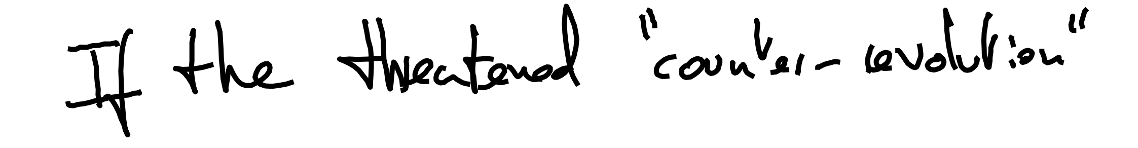
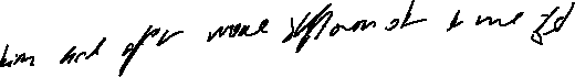
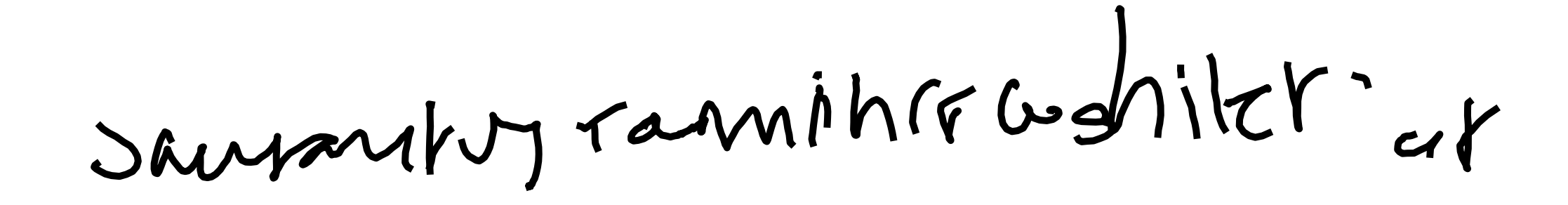
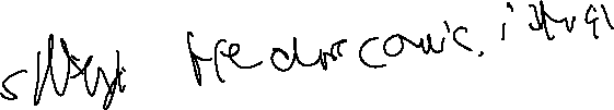
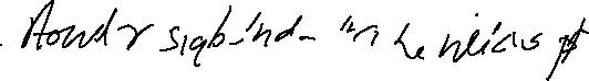
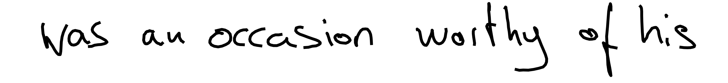
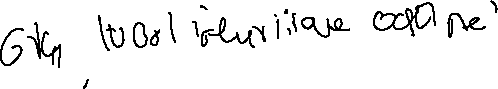
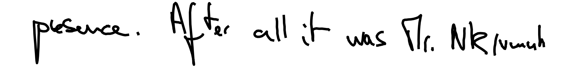
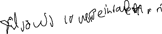
(a) Ground Truth

(b) RNN

(c) VRNN

(d) SWaveNet

Figure 3: Generated handwriting sample: (a) are the samples from the ground truth data. (b) (c), (d) are from RNN, VRNN and SWaveNet, respectively. Each line is one handwriting sample.

4.2 Handwriting and Human Motion Generation

Next, we evaluate the proposed model by visualizing generated samples from the trained model. The domain we choose is human handwriting, whose writing tracks are described by a sequential sample points. The following dataset is used to train the generative model:

IAM-OnDB (Liwicki and Bunke,, 2005): The human handwriting datasets contains 13,040 handwriting lines written by 500 writers. The writing trajectories are represented as a sequence of 3-dimension frames. Each frame is composed of two real-value numbers, which is $(x,y)$ coordinate for this sample point, and a binary number indicating whether the pen is touching the paper. The data preprocessing and division are same as (Graves,, 2013; Chung et al.,, 2015).

Method	IAM-OnDB
RNN (Chung et al.,, 2015)	1016
VRNN (Chung et al.,, 2015)	$\geq\textbf{1334}$
WaveNet	1021
SWaveNet	$\geq 1301$

Table 2: Log-likelihood results on IAM-OnDB dataset. The best result are highlighted in bold.

The quantitative results are reported in Table 2. SWaveNet achieves similar result compared with the best one, and still shows significant improvement to the vanilla WaveNet architecture. In Figure 3, we plot the ground truth samples and the ones randomly generated from different models. Compared with RNN and VRNN, SWaveNet shows clearer result. It is easy to distinguish the boundary of the characters, and we can obverse that more of them are similar to the English-characters, such as “is” in the fourth line and “her” in the last line.

4.3 Influence of Stochastic Latent Variables

The most prominent distinction between SWaveNet and RNN-based stochastic neural networks is that SWaveNet utilizes the dilated convolution layers to model multi-layer stochastic latent variables rather than one layer latent variables in the RNN models. Here, we perform the empirical study about the number of stochastic layers in SWaveNet model to demonstrate the efficiency of the design of multi-layers stochastic latent variables. The experiment is designed as follows. Firstly, we retain the total number of layers and only change the number of stochastic layers, namely the layer contains stochastic latent variables. More specifically, For a SWaveNet with $L$ layers and $S$ stochastic layers, $(S\leq L)$, we eliminate the stochastic latent variables in the bottom part, which is $\{z_{1:T,l};l<L-S\}$ in Eq.4. Then for each time stamp, when the model has $D$ dimension stochastic variables in total, each layer would have $\lfloor\frac{D}{S}\rfloor$ dimension stochastic variables. In this experiment, we set $D=500$.

We plot the experiment results in Figure 4. From the plots, we find that SWaveNet can achieve better performance with multiple stochastic layers. This demonstrates that it is helpful to encode the stochastic latent variables with a hierachical structure. And in the experiment on Blizzard and IAM-OnDB, we observe that the performance will decrease when the number of stochastic layers is large enough. Because too large number of stochastic layers would result in too small number of latent variables for a layer to memorize valuable information in different hierarchy levels.

We also study how the model performance would be influenced by the number of stochastic latent variables. Similar to previous one, we only tune the total number of stochastic latent variables and keep rest settings unchanged, which is 4 stochastic layers. The results are plotted in Figure 5. They demonstrate that Stochastic WaveNet would be benefited from even a small number of stochastic latent variables.

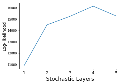
(a) Blizzard

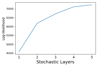
(b) TIMIT

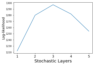
(c) IAM-OnDB

Figure 4: The influence of the number of stochastic layers of SWaveNet.

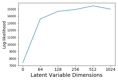
(a) Blizzard

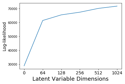
(b) TIMIT

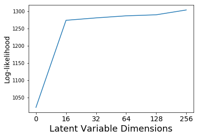
(c) IAM-OnDB

Figure 5: The influence of the number of stochastic latent variables of SWaveNet.

5 Conclusion

In this paper, we present a novel generative latent variable model for sequential data, named as Stochastic WaveNet, which injects stochastic latent variables into the hidden state of WaveNet. A new inference network structure is designed based on the characteristic of WaveNet architecture. Empirically results show state-of-the-art performances on various domains by leveraging additional stochastic latent variables. Simultaneously, the training process of WaveNet is greatly accelerated by parallell computation compared with RNN-based models. For future work, a potential research direction is to adopt the advanced training strategies (Goyal et al.,, 2017; Shabanian et al.,, 2017) designed for sequential stochastic neural networks, to Stochastic WaveNet.

References

- Bayer and Osendorfer, (2014) Bayer, J. and Osendorfer, C. (2014). Learning stochastic recurrent networks. arXiv preprint arXiv:1411.7610.
- Boulanger-Lewandowski et al., (2012) Boulanger-Lewandowski, N., Bengio, Y., and Vincent, P. (2012). Modeling temporal dependencies in high-dimensional sequences: Application to polyphonic music generation and transcription. arXiv preprint arXiv:1206.6392.
- Chung et al., (2014) Chung, J., Gulcehre, C., Cho, K., and Bengio, Y. (2014). Empirical evaluation of gated recurrent neural networks on sequence modeling. arXiv preprint arXiv:1412.3555.
- Chung et al., (2015) Chung, J., Kastner, K., Dinh, L., Goel, K., Courville, A. C., and Bengio, Y. (2015). A recurrent latent variable model for sequential data. In Advances in neural information processing systems, pages 2980–2988.
- Engel et al., (2017) Engel, J., Resnick, C., Roberts, A., Dieleman, S., Eck, D., Simonyan, K., and Norouzi, M. (2017). Neural audio synthesis of musical notes with wavenet autoencoders. arXiv preprint arXiv:1704.01279.
- Fabius and van Amersfoort, (2014) Fabius, O. and van Amersfoort, J. R. (2014). Variational recurrent auto-encoders. arXiv preprint arXiv:1412.6581.
- Fraccaro et al., (2016) Fraccaro, M., Sønderby, S. K., Paquet, U., and Winther, O. (2016). Sequential neural models with stochastic layers. In Advances in neural information processing systems, pages 2199–2207.
- Gan et al., (2015) Gan, Z., Li, C., Henao, R., Carlson, D. E., and Carin, L. (2015). Deep temporal sigmoid belief networks for sequence modeling. In Advances in Neural Information Processing Systems, pages 2467–2475.
- Goyal et al., (2017) Goyal, A., Sordoni, A., Côté, M.-A., Ke, N. R., and Bengio, Y. (2017). Z-forcing: Training stochastic recurrent networks. In Advances in Neural Information Processing Systems, pages 6716–6726.
- Graves, (2013) Graves, A. (2013). Generating sequences with recurrent neural networks. arXiv preprint arXiv:1308.0850.
- Gu et al., (2015) Gu, S., Ghahramani, Z., and Turner, R. E. (2015). Neural adaptive sequential monte carlo. In Advances in Neural Information Processing Systems, pages 2629–2637.
- Hochreiter and Schmidhuber, (1997) Hochreiter, S. and Schmidhuber, J. (1997). Long short-term memory. Neural computation, 9(8):1735–1780.
- Jordan et al., (1999) Jordan, M. I., Ghahramani, Z., Jaakkola, T. S., and Saul, L. K. (1999). An introduction to variational methods for graphical models. Machine learning, 37(2):183–233.
- Kingma and Ba, (2014) Kingma, D. P. and Ba, J. (2014). Adam: A method for stochastic optimization. arXiv preprint arXiv:1412.6980.
- Kingma and Welling, (2013) Kingma, D. P. and Welling, M. (2013). Auto-encoding variational bayes. arXiv preprint arXiv:1312.6114.
- Liwicki and Bunke, (2005) Liwicki, M. and Bunke, H. (2005). Iam-ondb-an on-line english sentence database acquired from handwritten text on a whiteboard. In Document Analysis and Recognition, 2005. Proceedings. Eighth International Conference on, pages 956–961. IEEE.
- Oord et al., (2016) Oord, A. v. d., Kalchbrenner, N., and Kavukcuoglu, K. (2016). Pixel recurrent neural networks. arXiv preprint arXiv:1601.06759.
- Oord et al., (2017) Oord, A. v. d., Li, Y., Babuschkin, I., Simonyan, K., Vinyals, O., Kavukcuoglu, K., Driessche, G. v. d., Lockhart, E., Cobo, L. C., Stimberg, F., et al. (2017). Parallel wavenet: Fast high-fidelity speech synthesis. arXiv preprint arXiv:1711.10433.
- Prahallad et al., (2013) Prahallad, K., Vadapalli, A., Elluru, N., Mantena, G., Pulugundla, B., Bhaskararao, P., Murthy, H., King, S., Karaiskos, V., and Black, A. (2013). The blizzard challenge 2013–indian language task. In Blizzard challenge workshop, volume 2013.
- Semeniuta et al., (2017) Semeniuta, S., Severyn, A., and Barth, E. (2017). A hybrid convolutional variational autoencoder for text generation. arXiv preprint arXiv:1702.02390.
- Shabanian et al., (2017) Shabanian, S., Arpit, D., Trischler, A., and Bengio, Y. (2017). Variational bi-lstms. arXiv preprint arXiv:1711.05717.
- Van Den Oord et al., (2016) Van Den Oord, A., Dieleman, S., Zen, H., Simonyan, K., Vinyals, O., Graves, A., Kalchbrenner, N., Senior, A., and Kavukcuoglu, K. (2016). Wavenet: A generative model for raw audio. arXiv preprint arXiv:1609.03499.
- (23) Yang, Z., Dai, Z., Salakhutdinov, R., and Cohen, W. W. (2017a). Breaking the softmax bottleneck: a high-rank rnn language model. arXiv preprint arXiv:1711.03953.
- (24) Yang, Z., Hu, Z., Salakhutdinov, R., and Berg-Kirkpatrick, T. (2017b). Improved variational autoencoders for text modeling using dilated convolutions. arXiv preprint arXiv:1702.08139.
- Yu and Koltun, (2015) Yu, F. and Koltun, V. (2015). Multi-scale context aggregation by dilated convolutions. arXiv preprint arXiv:1511.07122.