K2-260 b: a hot Jupiter transiting an F star, and K2-261 b: a warm Saturn around a bright G star

Abstract

We present the discovery and confirmation of two new transiting giant planets from the Kepler extended mission K2. K2-260 b is a hot Jupiter transiting a $V=12.7$ F6V star in K2 Field 13, with a mass and radius of $M_{\star}$$=1.39_{-0.06}^{+0.05}$ $\,M_{\odot}$ and $R_{\star}$$=1.69\pm 0.03$ $\,R_{\odot}$. The planet has an orbital period of $P=2.627$ days, and a mass and radius of $M_{P}=1.42^{+0.31}_{-0.32}$ $\,M_{\rm J}$ and $R_{P}=1.552^{+0.048}_{-0.057}$ $\,R_{\rm J}$. This is the first K2 hot Jupiter with a detected secondary eclipse in the Kepler bandpass, with a depth of $71\pm 15$ ppm, which we use to estimate a geometric albedo of $A_{g}\sim 0.2$. We also detected a candidate stellar companion at 0.6” from K2-260; we find that it is very likely physically associated with the system, in which case it would be an M5-6V star at a projected separation of $\sim 400$ AU. K2-261 b is a warm Saturn transiting a bright ($V=10.5$) G7IV/V star in K2 Field 14. The host star is a metal-rich ($\left[{\rm Fe}/{\rm H}\right]$$=0.36\pm 0.06$), mildly evolved $1.10_{-0.02}^{+0.01}$ $\,M_{\odot}$ star with $R_{\star}$$=1.65\pm 0.04$ $\,R_{\odot}$. Thanks to its location near the main sequence turn-off, we can measure a relatively precise age of $8.8_{-0.3}^{+0.4}$ Gyr. The planet has $P=11.633$ days, $M_{P}=0.223\pm 0.031$ $\,M_{\rm J}$, and $R_{P}=0.850^{+0.026}_{-0.022}$ $\,R_{\rm J}$, and its orbit is eccentric ($e=0.39\pm 0.15$). Its brightness and relatively large transit depth make this one of the best known warm Saturns for follow-up observations to further characterize the planetary system.

1 Introduction

Our knowledge of exoplanets has been revolutionised by the Kepler mission (Borucki et al., 2010), which during its prime mission discovered thousands of exoplanet candidates and confirmed exoplanets, providing powerful statistical measurements of planetary populations. After the failure of a second reaction wheel in 2013, the Kepler spacecraft began the K2 extended mission (Howell et al., 2014), pointing at a succession of fields around the ecliptic for $\sim 80$ days per field. The K2 mission has resulted in the detection of over 200 confirmed and validated planets, and even more planet candidates, to date (e.g., Mayo et al., 2018). On average K2 target stars are brighter than those from the Kepler prime mission, resulting in a population of planets that is more amenable to direct confirmation, and further observations to characterize these systems in more detail.

Building a large sample of planets that are characterized in detail will help to move the field of exoplanet population statistics beyond the parameters that have been probed by Kepler (principally planetary radius and orbital period; e.g., Burke et al., 2015). Large statistical studies of planetary atmospheres, spin-orbit misalignments, and other properties measurable via follow-up observations promise to set much more powerful constraints upon models of planet formation, migration, and evolution, and illuminate planetary astrophysics in general (e.g., Morton & Johnson, 2011; Sing et al., 2016).

Although a large number of planets and planet candidates around bright stars will soon be provided by the Transiting Exoplanet Survey Satellite (TESS; Ricker et al., 2015) mission, K2 planets are complementary to those that will be found by TESS. K2 observes in the ecliptic plane, which will not be covered by TESS during its prime mission. K2 is thus helping TESS to complete an all-sky catalogue of transiting short-period planets around relatively bright stars. Additionally, as K2 campaigns are significantly longer than TESS pointings ($\sim 80$ versus $\sim 27$ days), K2 is capable of finding longer-period planets than TESS typically will over most of the sky.

We present here the discovery, confirmation, and additional characterization of two new transiting planets from K2: K2-260 b and K2-261 b. K2-260 b is a hot Jupiter transiting a $V=12.7$ mid-F star, while K2-261 b is a warm Saturn transiting a $V=10.6$ late-G star near the main sequence turn-off. Both are amenable to further observations, and can add to the number of giant planets characterized in detail.

These planets were discovered and characterized as part of the KESPRINT collaboration to find planets using K2. Our team has confirmed and characterized over two dozen transiting planets using K2, including hot Jupiters (e.g., Grziwa et al., 2016; Hirano et al., 2016b; Johnson et al., 2016), longer-period giant planets (e.g., Smith et al., 2017; Van Eylen et al., 2018), ultra-short-period planets (e.g., Dai et al., 2017; Smith et al., 2018), multiplanet systems (e.g., Gandolfi et al., 2017; Niraula et al., 2017), as well as other planets (e.g., Narita et al., 2017).

2 Observations

2.1 K2 Photometry

The Kepler spacecraft observed K2 Field 13 from 2017 March 8 to May 27 UT, a span of 79.0 days. Field 13 is centred at RA$=04^{h}51^{m}11^{s}$, Dec$=+20^{\circ}47^{\prime}11^{\prime\prime}$ (J2000.0). The star EPIC 246911830 (K2-260) was proposed for observations by programs GO13122 (P.I. Howard) and GO13071 (P.I. Charbonneau). K2 Field 14 was observed for 70.4 days between 2017 May 31 and August 9 UT. Field 14 is centred at RA$=10^{h}42^{m}44^{s}$, Dec$=+06^{\circ}51^{\prime}06^{\prime\prime}$ (J2000.0). EPIC 201498078 (K2-261) was proposed for observations by programs GO14009 (P.I. Charbonneau), GO14020 (P.I. Adams), GO14021 (P.I. Howard), and GO14028 (P.I. Cochran).

We conducted three parallel searches of all of the light curves from Campaigns 13 and 14 for transits using three separate methodologies. One method utilizes aperture photometry to extract light curves from the K2 raw pixel data, and decorrelates the light curves based upon the centroid motion to account for the roll of the spacecraft, as described in Dai et al. (2016). We then perform a standard BLS (Box Least Squares; Kovács et al., 2002) transit search upon the light curves.

The other two methods both used the K2 light curves for Campaigns 13 and 14 as extracted and corrected for systematics per Vanderburg & Johnson (2014) as provided by A. Vanderburg. We used the exotrans package (Grziwa et al., 2012) in order to search the light curves for transits. This package utilizes the varlet (Grziwa & Pätzold, 2016) wavelet-based filtering technique in order to remove stellar and systematic variability from the light curves, along with a BLS transit search algorithm. If a transit is detected, it is removed using another wavelet-based filtering technique, phalet, and the light curve searched again for additional transits using BLS.

We also used the code dst (Cabrera et al., 2012) to search for transits in the Vanderburg & Johnson (2014) light curves. This algorithm is conceptually similar to BLS, but uses a more realistic transit shape rather than an inverted tophat for the transit search, accounts for the potential presence of transit timing variations, and uses improved statistical methods.

All three search techniques detected significant transits for both K2-260 (with a period of $\sim 2.6$ days and a depth of $\sim 1$ per cent) and K2-261 (with a period of $\sim 11.6$ days and a depth of $\sim 0.3$ per cent); indeed, the transits are easily visible by eye in the detrended K2 light curves (Fig. 1). None of the algorithms identified any additional candidate transits for either star.

We list the coordinates, magnitudes, and other identifying information for K2-260 and K2-261 in Table 1.

Table 1: Coordinates, magnitudes, and kinematics of K2-260 and K2-261

Parameter	K2-260	K2-261	Reference
Coordinates and Identifiers
RA (J2000.0)	$05^{h}07^{m}28^{s}.16$	$10^{h}52^{m}07^{s}.78$	1
Dec (J2000.0)	$+16^{\circ}52^{\prime}03^{\prime\prime}.78$	$+00^{\circ}29^{\prime}36^{\prime\prime}.07$	1
EPIC	246911830	201498078
TYC		255-257-1
UCAC4	535-011514	453-051151
2MASS	J05072816+1652037	J10520778+0029359
AllWISE	J050728.15+165203.7	J105207.76+002935.6
Magnitudes
$Kp$ (mag)	$12.465$	$10.451$	1
$G$ (mag)	$12.467$	$10.459$	2
$Bp$ (mag)	$12.798$	$10.872$	2
$Rp$ (mag)	$11.973$	$9.917$	2
$B$ (mag)	$13.217\pm 0.042$	$11.561\pm 0.086$	1
$V$ (mag)	$12.69\pm 0.11$	$10.612\pm 0.059$	1
$g$ (mag)	$12.881\pm 0.010$	$10.979\pm 0.010$	1
$r$ (mag)	$12.449\pm 0.030$	$10.402\pm 0.020$	1
$i$ (mag)	$12.287\pm 0.010$	$10.226\pm 0.020$	1
$J$ (mag)	$11.400\pm 0.023$	$9.337\pm 0.030$	1
$H$ (mag)	$11.189\pm 0.032$	$8.920\pm 0.042$	1
$K$ (mag)	$11.093\pm 0.021$	$8.890\pm 0.022$	1
$W1$ (mag)	$11.039\pm 0.023$	$8.828\pm 0.023$	3
$W2$ (mag)	$11.036\pm 0.021$	$8.897\pm 0.020$	3
$W3$ (mag)	$10.895\pm 0.129$	$8.819\pm 0.031$	3
$W4$ (mag)	$>9.006$	$>8.281$	3
$B-V$ (mag)	$0.53\pm 0.12$	$0.95\pm 0.10$	4
$J-K$ (mag)	$0.307\pm 0.031$	$0.447\pm 0.037$	4
Distance and Velocities
$\mu_{\mathrm{RA}}$ (mas yr-1)	$0.667\pm 0.078$	$-23.664\pm 0.075$	2
$\mu_{\mathrm{Dec}}$ (mas yr-1)	$-6.045\pm 0.051$	$-44.171\pm 0.068$	2
$\Pi$ (mas)	$1.479\pm 0.042$	$4.660\pm 0.043$	2
$d$ (pc)	$676\pm 19$	$214.6\pm 2.0$	2
$v_{\mathrm{rad}}$ ($\rm km\ s^{-1}$)	$29.1\pm 2.7$	$3.28\pm 0.52$	2
$U$ ($\rm km\ s^{-1}$)	$15.8\pm 2.6$	$-8.99\pm 0.13$	This Work
$V$ ($\rm km\ s^{-1}$)	$-6.15\pm 0.57$	$-29.14\pm 0.49$	This Work
$W$ ($\rm km\ s^{-1}$)	$-9.46\pm 0.73$	$-21.81\pm 0.50$	This Work
Notes: the mean stellar radial velocity $v_{\mathrm{rad}}$ is measured from our FIES spectra for K2-260 and from our McDonald reconnaissance spectrum for K2-261. The quoted $UVW$ velocities are in the LSR frame and use the LSR definition and $UVW$ frame of Coşkunoǧlu et al. (2011). References: 1: Ecliptic Plane Input Catalog (EPIC: Huber et al. 2016; https://archive.stsci.edu/k2/epic/search.php); 2: Gaia DR2 (Gaia Collaboration et al., 2018); 3: AllWISE (Cutri et al., 2013); 4: calculated from literature values given earlier in this table.

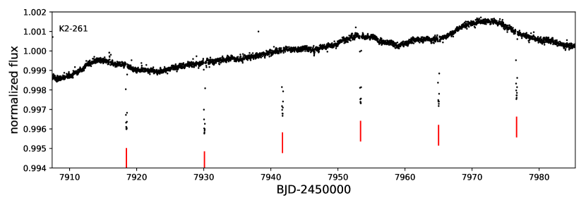
Figure 1: K2 light curves of K2-260 (top), and K2-261 (bottom), as detrended and corrected for systematics by Vanderburg & Johnson (2015). Note the rotational variability of K2-260, which is discussed in §3.4. For both systems we remove the stellar and instrumental variations prior to fitting the transits. Vertical bars mark the locations of each transit.

2.2 High-resolution imaging

In order to test for the presence of nearby stars which could dilute the transit depth and perhaps indicate that the planet candidate could be a false positive, we obtained high-resolution imaging observations of both K2-260 and K2-261.

We obtained high-resolution images of K2-260 using the Infrared Camera and Spectrograph (IRCS: Kobayashi et al., 2000) with the adaptive optics (AO) system AO188: (Hayano et al., 2010) mounted on the 8.2 m Subaru telescope on 2018 March 29 UT. For the AO imaging, we adopted the fine-sampling mode (20 mas per pixel) and $H-$band filter. Short exposure, unsaturated frames (0.6 s $\times$ 3 coadds for each position) were first secured with five-point dithering, which are used for the absolute flux calibration. We then ran long-exposure sequences (15 s $\times$ 3 coadds for each position) adopting the same five-point dithering, resulting in saturated frames of K2-260 to look for faint nearby companions. The total exposure time amounted to 450 s for the saturated frames.

Following Hirano et al. (2016a), we applied dark subtraction, bad pixel interpolation, flat fielding, and distortion correction to the raw IRCS frames. The unsaturated and saturated frames were then respectively aligned and combined to obtain the final reduced images. The combined unsaturated image of K2-260 showed that the AO-corrected full width at half maximum (FWHM) of the target’s point spread function was $0\aas@@fstack{\prime\prime}10$.

Visual inspection of the combined saturated image suggested a presence of a faint source in the south-east of K2-260  with a separation of $\sim 0\aas@@fstack{\prime\prime}6$ (see the inset of Figure 2). In order to estimate the contrast of this candidate companion (CC), we performed aperture photometry for K2-260 and its CC with its aperture radius being the FWHM of the target. For the CC’s photometry, we applied high-pass filtering (with a width of $4\times\mathrm{FWHM}$) to the saturated image to suppress the halo of the primary star.

High-pass filtering suppresses the halo of the primary star, but it also reduces the CC’s flux. In order to estimate the flux loss from the high-pass filtering, we implemented a simulation in which an artificial companion’s signal is injected into the saturated image with the same angular separation (but with different position angles). The mock data were analysed using the same steps above to measure the artificial companion’s flux. As a result, we found that approximately 25% of the injected signal was lost by high-pass filtering. Taking into account this flux loss, we measured the CC’s magnitude and its position. Table 2 summarizes the measured CC properties. To evaluate the detection level of the CC, we also drew the 5$\sigma$ contrast curve based on the scatter of the flux count in the annulus as a function of angular separation from K2-260. Figure 2 implies that at the separation of $\sim 0\aas@@fstack{\prime\prime}6$, a 5$\sigma$ contrast of $\Delta H=7.3$ mag was achieved, and thus the CC was detected with $>5\sigma$.

The companion has a flux ratio of $0.00200\pm 0.00033$, corresponding to $\Delta H=6.75\pm 0.18$ mag. It is located at an angular separation of $0.605\pm 0.026$ arcsec and a position angle of $151.8^{\circ}\pm 2.5^{\circ}$. If the companion were to be physically associated with K2-260, this corresponds to a projected physical separation of $409\pm 21$ AU at the 676 pc distance of K2-260 (Gaia Collaboration et al., 2018).

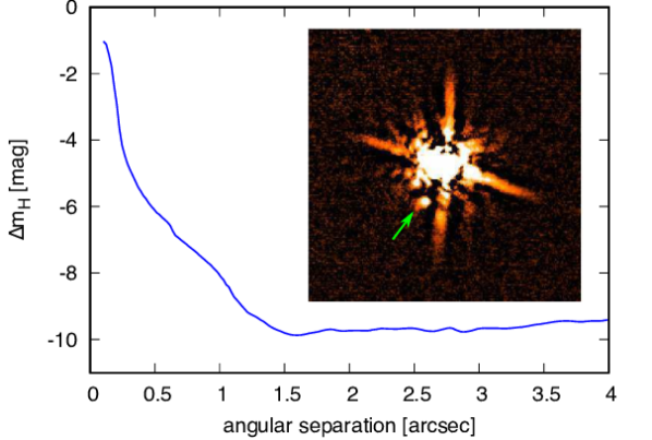
Figure 2: $H$-band $5\sigma$ contrast curve of K2-260 from IRCS. Inset: high-pass filtered image. The candidate companion is marked with an arrow.

Table 2: Properties of the Candidate Companion to K2-260

Parameter	Unit	Value	Uncertainty
Measured Parameters
$\rho$	arcsec	$0.605$	$0.026$
PA	∘	$151.8$	$2.5$
$f_{\mathrm{CC}}/f_{A}$		$0.00200$	$0.00033$
$\Delta H$	mag	$6.75$	$0.18$
Estimated Parameters
$a_{\perp}$	AU	$409$	$21$
$M_{\mathrm{CC}}$	$\,M_{\odot}$	$0.145$	$0.015$
Spec. Type		M5-6V
Notes: $f_{\mathrm{CC}}/f_{A}$ is the flux ratio of the companion with respect to the primary in the $H$ band. $a_{\perp}$ is the projected separation.

We obtained the observations of K2-261using the FastCam lucky imaging camera (Oscoz et al., 2008) on the 1.52 m Telescopio Carlos Sánchez at Teide Observatory, Spain. FastCam is a very low noise and fast readout speed electron multiplying CCD camera with $512\times 512$ pixels (with a physical pixel size of 16 $\mu$m, and a field of view of $21.2\times 21.2$ arcsec). We observed K2-261 on 2018 March 20 UT, obtaining 5,000 individual frames with 50 ms exposure times through a clear filter. The conditions were clear with 1.7 arcsec seeing and we obtained a Strehl ratio of 0.06. In order to construct a high resolution, long-exposure image, each individual frame was bias-subtracted, aligned and co-added and then processed with the FastCam dedicated software (Labadie et al., 2010; Jódar et al., 2013). Fig. 3 shows the contrast curve that was computed based on the scatter within the annulus as a function of angular separation from the target centroid. We used a high resolution image constructed by co-addition of the $30$ per cent best images, so that it had a 75 s total exposure time, which achieved a $5\sigma$ detection limit better than $\sim 6$ magnitudes outside 3 arcsec separation, and better than $\sim 3$ magnitudes outside $\sim 50$ mas. We did not detect any secondary sources within these limits inside 6.0 arcsec of K2-261.

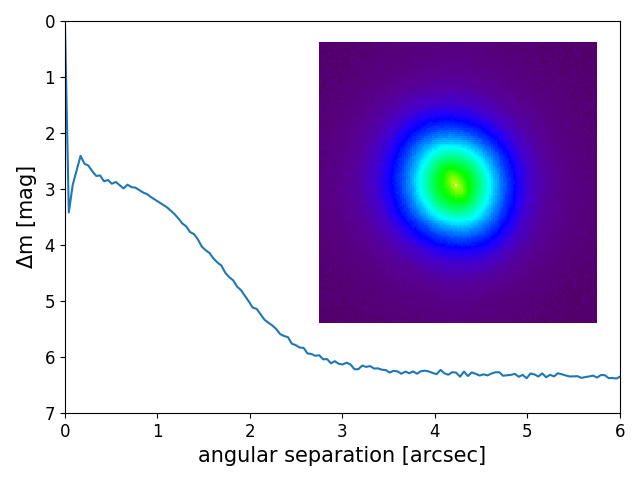
Figure 3: Clear filter contrast curve as a function of angular separation up to $6.0$ arcsec from K2-261 obtained with the FastCam camera at TCS. The solid line indicates the $5\sigma$ detection limit for secondary sources, none of which are detected. The inset shows the $6\times 6$ arcsec combined image of K2-261. North is up and East is left.

2.3 Ground-based photometry

In order to perform additional false positive vetting of K2-260, we obtained follow-up ground-based photometric observations of several transits. We obtained these observations with two different facilities.

First, we observed with the DEMONEXT automated 0.51 m robotic telescope (Villanueva et al., 2018), located at Winer Observatory, Arizona, USA. We observed the transits of 2017 November 14 and 22 UT in alternating Sloan $g$ and $i$ filters, using 20 s exposures in each band, and binned together each set of five consecutive exposures in each band in order to increase the signal-to-noise. We obtained these pseudo-simultaneous multi-band observations in order to verify that the transit is achromatic, excluding certain blended eclipsing binary scenarios. The observations were obtained through thin clouds, degrading the expected photometric performance, but nonetheless we detect the transits of K2-260 b. The transits in both $g$ and $i$ appear to be slightly shallower than that in the K2 light curve; however, given the precision of the DEMONEXT data and systematic uncertainties in the depth associated with detrending the DEMONEXT data, we do not consider these differences to be significant. Furthermore, if these depth differences were due to dilution by another star, we would not expect both bands to exhibit smaller transit depths than the K2 data unless the contaminating star were to be of a very similar $T_{\rm eff}$ to K2-260. Although the DEMONEXT data are much less precise than the K2 photometry, we nonetheless include them in our fits (§3.3) as the longer time baseline improves the precision of our ephemeris measurement. We show these data in Fig. 6.

We additionally obtained observations of the partial transits of 2018 February 18 and March 10 UT using the Multicolor Simultaneous Camera for studying Atmospheres of Transiting exoplanets 2 (MuSCAT2; Narita et al., 2018), which is also on the Telescopio Carlos Sánchez. MuSCAT2 observes simultaneously in the $g$, $r$, $i$, and $z$ bands, using a set of dichroics to split the light between four separate cameras. The transit depth in all four MuSCAT2 bands for both partial transits is consistent with that from K2, giving no evidence for a chromatic transit depth and indicating that the inconsistent transit depths in the DEMONEXT data are indeed likely due to systematics and problems with the detrending. We also include the MuSCAT2 data in our simultaneous fits. We also show these data in Fig. 6.

The transit of K2-261 b is shallower than that of K2-260 b and not as easily detectable from the ground. We therefore did not obtain any follow-up transit photometry of K2-261 b.

2.4 High-resolution spectroscopy

After identification of the transiting planet candidates around K2-260 and K2-261, we obtained reconnaissance spectroscopy observations in order to measure the stellar parameters and rule out obvious false positive scenarios (such as eclipsing binaries with two sets of strong lines). We obtained these spectra with the 2.7 m Harlan J. Smith Telescope at McDonald Observatory, Texas, USA, and its Robert G. Tull coudé spectrograph (Tull et al., 1995). We used the spectrograph in its TS23 configuration, which gives a spectral resolving power of $R=60,000$ over the range 3750-10200 Å, with complete spectral coverage below 5691 Å. We obtained a spectrum of each K2-260 and K2-261 with a signal-to-noise ratio (SNR) per-resolution element of 35 and 50 at 5650 Å for K2-260 and K2-261, respectively. We measured stellar parameters from these spectra using the Kea spectral analysis tool (Endl & Cochran, 2016).

The reconnaissance spectra indicated that both K2-260 and K2-261 were good targets for precise radial velocity (RV) follow-up in order to confirm these planet candidates and measure their masses: both stars are relatively slowly rotating and have high surface gravity, and neither of them show any evidence of multiple lines in the spectra. We obtained precise RVs with three different facilities; these have higher SNRs and so superseded the reconnaissance spectra in our further analyses.

We obtained observations of both K2-260 and K2-261 using the FIbre-fed Échelle Spectrograph (FIES; Frandsen & Lindberg, 1999; Telting et al., 2014) on the 2.56 m Nordic Optical Telescope (NOT) at the Observatorio del Roque de los Muchachos, La Palma, Spain. We used FIES’ high-res mode, which provides spectra with $R=67,000$ over the range 3600-9000 Å. We used the same observing strategy as in Gandolfi et al. (2015); at each observation epoch we obtained three consecutive exposures to facilitate cosmic ray removal, bracketed by $120-180$-second ThAr exposures in order to trace any drift of the spectrograph. We obtained eighteen RVs of K2-260 with FIES between 2017 November 16 and 2018 March 11 UT, and twelve of K2-261 between 2017 December 26 and 2018 February 15 UT, as part of the observing programs 56-010, 56-112, and 56-209.

We also obtained observations of both targets using the High Accuracy Radial velocity Planet Searcher for the Northern hemisphere (HARPS-N; Cosentino et al., 2012) spectrograph on the 3.58 m Telescopio Nazionale Galileo (TNG), also at La Palma. HARPS-N is a fibre-fed cross-dispersed échelle spectrograph, and provides spectra with $R=115,000$ over the range 3830-6900 Å. We observed K2-261 nine times between 2017 December 27 and 2018 February 22 UT, and K2-260 twice on 2018 February 19 UT, as part of the programs A36TAC_12, CAT17B_99, and OPT17B_059. We did not utilize the two HARPS-N RVs for K2-260 in our fits as their poor phase coverage results in little constraining power on the fits. Additionally, one HARPS-N RV of K2-261 was excluded from the fit due to poor signal-to-noise.

Finally, we obtained observations of K2-261 using the High Accuracy Radial velocity Planet Searcher (HARPS; Mayor et al., 2003). The spectrograph is essentially identical to HARPS-N, and is located on the ESO 3.6 m telescope at La Silla Observatory, Chile. We obtained ten RV observations of K2-261 using HARPS between 2018 January 25 and May 13 UT under the programs 0100.C.0808 and 0101.C-0829. One HARPS RV was excluded from our fits due to an incorrect flux correction by the HARPS pipeline.

For both HARPS and HARPS-N we reduced the data using the dedicated off-line pipelines and extracted the RVs via cross-correlation with a G2 numerical mask (Baranne et al., 1996; Pepe et al., 2002). For FIES we reduced the data as described in Gandolfi et al. (2015), using standard IRAF and IDL routines, which include bias subtraction, flat fielding, order tracing and extraction, and wavelength calibration. The FIES RVs of K2-260 were derived by cross-correlating the observed spectra against a high SNR (>300) spectrum of the RV standard star HD 50692 observed with the same instrument set-up as K2-260. For K2-261, relative RVs were extracted by cross-correlating the observed FIES data against the first stellar spectrum.

We show these data in Fig. 4, and list all of our RV measurements in Table 3, along with the cross-correlation function bisector span (BIS) and full width at half maximum (FWHM), and the Ca ii H & K chromospheric activity index $\log R^{\prime}_{\mathrm{HK}}$ (the latter measured only from the HARPS-N and HARPS spectra). We do not find any significant correlation between the RV measurements and the BIS, as well as between the RVs and the FWHMs, for either target, and we robustly detect the stellar RV variations induced by both transiting objects, confirming both K2-260 b and K2-261 b as bona fide planets.

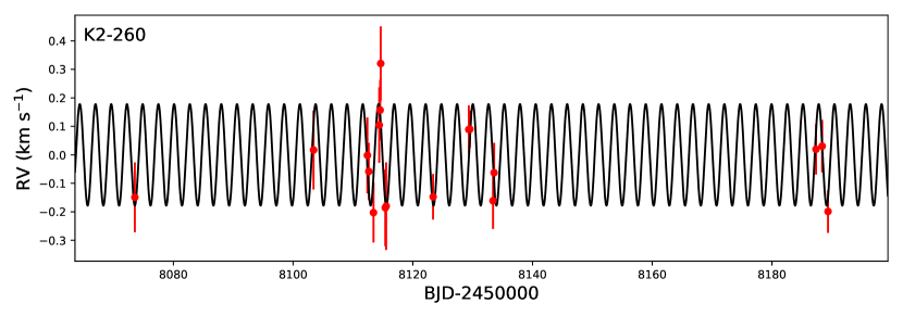
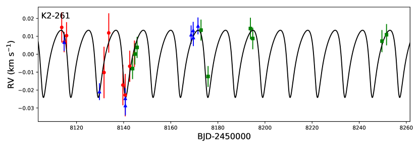
Figure 4: Radial velocity measurements of K2-260 (top) and K2-261 (bottom), along with the best-fit orbit models computed in §3.3. Data from FIES are shown as circles (red in the online version), HARPS-N as triangles (blue online), and HARPS as squares (green online). The error bars incorporate both the internal RV errors and the best-fit RV jitter.

Table 3: Radial velocity measurements of K2-260 and K2-261

BJDTDB	RV	$\sigma_{\mathrm{RV}}$	BIS	FWHM	$\log R^{\prime}_{\mathrm{HK}}$	$\sigma_{\log R^{\prime}_{\mathrm{HK}}}$	$T_{\mathrm{exp}}$	SNR	Instrument
	($\rm km\ s^{-1}$)	($\rm km\ s^{-1}$)	($\rm km\ s^{-1}$)	($\rm km\ s^{-1}$)			(s)
K2-260
$2458073.56279$	$28.9213$	$0.1196$	$0.4946$	$28.3623$			$3600$	$23$	FIES
$2458103.41726$	$29.0872$	$0.1358$	$0.5607$	$28.0208$			$3600$	$25$	FIES
$2458112.41796$	$29.0684$	$0.1306$	$0.7535$	$28.5843$			$3600$	$21$	FIES
$2458112.64764$	$29.0119$	$0.0966$	$0.2418$	$28.1836$			$3600$	$28$	FIES
$2458113.42787$	$28.8675$	$0.1017$	$0.4048$	$28.2302$			$3600$	$28$	FIES
$2458114.38939$	$29.1748$	$0.1296$	$0.7658$	$28.3094$			$3600$	$20$	FIES
$2458114.54165$	$29.2274$	$0.1025$	$0.6633$	$28.4909$			$3600$	$24$	FIES
$2458114.63722$	$29.3908$	$0.1274$	$0.5007$	$28.2135$			$3600$	$18$	FIES
$2458115.40316$	$28.8845$	$0.1320$	$0.6163$	$28.4217$			$3600$	$21$	FIES
$2458115.55094$	$28.8900$	$0.1512$	$0.6702$	$28.1998$			$3600$	$14$	FIES
$2458123.39303$	$28.9230$	$0.0753$	$0.2370$	$28.1771$			$3600$	$29$	FIES
$2458129.35492$	$29.1592$	$0.0805$	$0.2508$	$29.0288$			$3600$	$27$	FIES
$2458129.53697$	$29.1604$	$0.0599$	$0.2017$	$28.1717$			$3600$	$26$	FIES
$2458133.39617$	$28.9090$	$0.0948$	$0.3268$	$28.5724$			$3600$	$28$	FIES
$2458133.57782$	$29.0075$	$0.1015$	$0.2893$	$28.2565$			$3600$	$26$	FIES
$2458187.35731$	$29.0897$	$0.0843$	$0.3350$	$29.2858$			$3600$	$25$	FIES
$2458188.38929$	$29.1007$	$0.0879$	$0.7315$	$28.1793$			$3600$	$26$	FIES
$2458189.36976$	$28.8715$	$0.0699$	$0.1347$	$28.8898$			$3600$	$24$	FIES
$2458169.40257$	$29.279$	$0.052$	$-1.206$	$26.5556$	$-4.594$	$0.062$	$3600$	$18$	HARPS-N
$2458169.44866$	$29.366$	$0.050$	$-6.231$	$27.0874$	$-4.674$	$0.071$	$3600$	$19$	HARPS-N
K2-261
$2458113.71551$	$0.0000$	$0.0079$	$0.0005$	$12.4310$			$3600$	$52$	FIES
$2458114.74539$	$-0.0052$	$0.0049$	$0.0089$	$12.3931$			$3600$	$57$	FIES
$2458115.75979$	$-0.0045$	$0.0068$	$0.0065$	$12.4364$			$3600$	$63$	FIES
$2458131.68086$	$-0.0300$	$0.0140$	$0.0130$	$12.4362$			$3600$	$29$	FIES
$2458133.67474$	$-0.0068$	$0.0095$	$0.0081$	$12.4448$			$3600$	$38$	FIES
$2458139.68280$	$-0.0340$	$0.0110$	$0.0360$	$12.4553$			$3600$	$37$	FIES
$2458140.68126$	$-0.0350$	$0.0120$	$0.0130$	$12.3920$			$3600$	$38$	FIES
$2458142.59534$	$-0.0284$	$0.0084$	$0.0139$	$12.4582$			$3600$	$43$	FIES
$2458144.59629$	$-0.0115$	$0.0068$	$0.0082$	$12.3859$			$3600$	$44$	FIES
$2458146.69263$	$0.0020$	$0.0110$	$0.0200$	$12.4276$			$3600$	$35$	FIES
$2458163.53606$	$-0.0179$	$0.0056$	$0.0165$	$12.4710$			$3600$	$56$	FIES
$2458164.59738$	$-0.0369$	$0.0050$	$-0.0041$	$12.4503$			$3600$	$55$	FIES
$2458114.75801$	$3.3424$	$0.0019$	$-0.0058$	$7.4426$	$-5.139$	$0.043$	$900$	$43$	HARPS-N
$2458129.73171$	$3.3148$	$0.0011$	$-0.0087$	$7.4581$	$-5.129$	$0.019$	$1800$	$68$	HARPS-N
$2458140.70807$	$3.3110$	$0.0034$	$-0.0133$	$7.4584$	$-5.204$	$0.163$	$1200$	$29$	HARPS-N
$2458140.72396$	$3.3070$	$0.0030$	$0.0024$	$7.4599$	$-4.943$	$0.091$	$1200$	$33$	HARPS-N
$2458168.63918$	$3.3465$	$0.0025$	$-0.0006$	$7.4408$	$-5.169$	$0.066$	$2100$	$36$	HARPS-N
$2458169.52666$	$3.3489$	$0.0014$	$-0.0066$	$7.4393$	$-5.077$	$0.026$	$3300$	$55$	HARPS-N
$2458169.59477$	$3.3449$	$0.0013$	$-0.0069$	$7.4464$	$-5.056$	$0.021$	$3300$	$60$	HARPS-N
$2458169.70060^{\dagger}$	$3.2810^{\dagger}$	$0.0440^{\dagger}$	$-0.1753^{\dagger}$	$7.2957^{\dagger}$	$-4.545^{\dagger}$	$0.451^{\dagger}$	$267^{\dagger}$	$4^{\dagger}$	HARPS-N†
$2458171.56866$	$3.3514$	$0.0011$	$-0.0065$	$7.4418$	$-5.111$	$0.017$	$1500$	$70$	HARPS-N
$2458143.78984$	$3.3331$	$0.0013$	$-0.0093$	$7.4954$	$-5.177$	$0.031$	$1500$	$64$	HARPS
$2458144.77455$	$3.3412$	$0.0014$	$-0.0054$	$7.4928$	$-5.207$	$0.039$	$1200$	$58$	HARPS
$2458145.71595$	$3.3449$	$0.0014$	$-0.0050$	$7.4817$	$-5.208$	$0.040$	$1500$	$57$	HARPS
$2458171.71521^{\dagger}$	$3.3438^{\dagger}$	$0.0016^{\dagger}$	$-0.0179^{\dagger}$	$7.6649^{\dagger}$			$1500^{\dagger}$	$71^{\dagger}$	HARPS†
$2458172.84902$	$3.3546$	$0.0012$	$-0.0030$	$7.4881$	$-5.255$	$0.043$	$1500$	$67$	HARPS
$2458175.84594$	$3.3287$	$0.0011$	$-0.0056$	$7.4916$	$-5.184$	$0.035$	$1500$	$76$	HARPS
$2458193.81413$	$3.3555$	$0.0018$	$-0.0038$	$7.4958$	$-5.081$	$0.046$	$1200$	$46$	HARPS
$2458194.80916$	$3.3499$	$0.0018$	$0.0030$	$7.4968$	$-5.010$	$0.040$	$1200$	$47$	HARPS
$2458249.65186$	$3.3484$	$0.0023$	$0.0053$	$7.5094$	$-5.303$	$0.099$	$1200$	$37$	HARPS
$2458251.59291$	$3.3520$	$0.0016$	$-0.0014$	$7.4957$	$-5.194$	$0.048$	$1200$	$52$	HARPS
Notes: We do not use the two HARPS-N spectra of K2-260 in our fits as the phase coverage is insufficient to provide good constraints upon the fits, and also excluded the two spectra marked as † from our fits due to low signal-to-noise and other problems. The FIES RVs of K2-261 are measured with respect to the first spectrum, the RV of which is arbitrarily set to zero. See Table 5 for the best-fit RV offsets for each dataset. We did not measure the activity index $\log R^{\prime}_{\mathrm{HK}}$ from our FIES spectra as our pipeline is not configured to do so. The bisector spans quoted for the HARPS-N data on K2-260 are likely inaccurate as they were derived using the pipeline G2 CCF mask, which is not a good match to the F6 spectral type of the target. The quoted signal-to-noise ratio (SNR) is the per-pixel SNR measured at 5500 Å.

3 Analysis

3.1 Spectral analysis and stellar parameters

In order to derive more precise stellar parameters than were found using our reconnaissance spectra (§2.4), we analysed our co-added HARPS-N spectra of K2-261, and our co-added FIES spectra of K2-260. The spectroscopic analysis was performed within the iSpec framework (Blanco-Cuaresma et al., 2014). We derived spectroscopic parameters ($T_{\text{eff}}$, $\log g$, $\left[{\rm Fe}/{\rm H}\right]$, $v_{\text{mic}}$) by fitting synthetic spectra computed using moog (Sneden, 1973) and ATLAS9 model atmospheres (Castelli & Kurucz, 2004) to the co-added spectra. We computed the broadening function by convolving the observed spectrum with a sharp-lined template. The broadening function was fitted with a broadened line profile to obtain $v\sin{i_{\star}}$ and the macroturbulent velocity $v_{\text{mac}}$. For K2-260 we fixed the microturbulent velocity $v_{\text{mic}}$ using the values from Doyle et al. (2014) expected based upon the $T_{\rm eff}$, $\log{g_{\star}}$  and $\left[{\rm Fe}/{\rm H}\right]$ in the fit.

For K2-260 we could not obtain a good measurement of $\log{g_{\star}}$ from the spectra due to insufficient signal-to-noise and the moderate rotational broadening ($v\sin{i_{\star}}$$=16.0\pm 2.0$ $\rm km\ s^{-1}$). We therefore estimated $\log{g_{\star}}=4.15_{-0.04}^{+0.02}$ using the mean stellar density derived from the circular-orbit transit fit (§3.3) and basta isochrones (Silva Aguirre et al., 2015) with a flat prior over the range $5500$ K$<$$T_{\rm eff}$$<7500$ K. We fixed $\log{g_{\star}}$ to this value in the spectral analysis as the uncertainties are much smaller than generally obtainable from spectroscopy alone. For both stars we leveraged the precise Gaia DR2 parallaxes (Gaia Collaboration et al., 2016, 2018) to fit the stellar SEDs, using the $BVgriJHK$-band photometry listed in Table 1. For K2-260 we included reddening of $E(B-V)=0.18\pm 0.006$ from Green et al. (2018), while for K2-261 we assumed $E(B-V)=0$. The stellar parameters for the two stars are listed in Table 4.

We inferred the stellar masses, radii, and ages using the basta code to fit the measured $T_{\rm eff}$, $\left[{\rm Fe}/{\rm H}\right]$, and mean stellar density to an isochrone grid from the BaSTI database computed using the franec stellar evolutionary models (Pietrinferni et al., 2004). Our derived parameters are also listed in Table 4. Thanks to the location of both stars near the main sequence turn-off we are able to measure relatively precise ages of $1.9\pm 0.3$ Gyr for K2-260 and $8.8_{-0.3}^{+0.4}$ Gyr for K2-261. We show the position of both stars in the H-R diagram in Fig. 5.

We estimated spectral types for the stars based upon the $T_{\rm eff}$-spectral type calibration of Pecaut & Mamajek (2013), obtaining spectral types of F6 and G7, respectively. K2-261 lies just past the main sequence turn-off, and so we quote a spectral type of G7IV/V, while K2-260 lies at the main sequence turn-off, resulting in a spectral type of F6V.

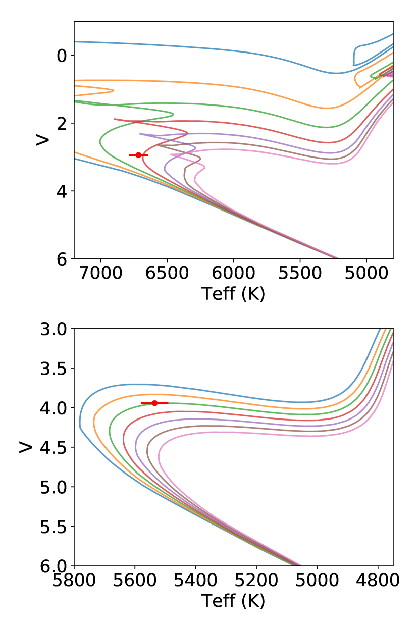
Figure 5: H-R diagrams showing K2-260 (top) and K2-261 (bottom). For K2-260 the lines show BaSTI isochrones of, from top to bottom, 0.5 (coloured blue online), 1.0 (orange), 1.5 (green), 2.0 (red), 2.5 (purple), 3.0 (brown), and 3.5 (pink) Gyr for $\left[{\rm Fe}/{\rm H}\right]$$=-0.1$, while for K2-261the lines show isochrones with ages of, from left to right, 7 (blue), 8 (orange), 9 (green), 10 (red), 11 (purple), 12 (brown), and 13 (pink) Gyr for $\left[{\rm Fe}/{\rm H}\right]$$=+0.4$. Coincidentally, both K2-260 and K2-261 are located near the main sequence turn-off, although K2-261 has already passed this point whereas K2-260 is only now reaching it.

Table 4: Stellar parameters of K2-260 and K2-261

Parameter	K2-260	K2-261
Measured Parameters
$T_{\rm eff}$ (K)	$6367\pm 250$	$5537\pm 71$
$\log{g_{\star}}$(cgs)	$4.15$ (fixed)	$4.21\pm 0.11$
$\left[{\rm Fe}/{\rm H}\right]$ (dex)	$-0.14\pm 0.15$	$0.36\pm 0.06$
$v\sin{i_{\star}}$ ($\rm km\ s^{-1}$)	$16.0\pm 2.0$	$2.8\pm 0.5$
$v_{\mathrm{mic}}$ ($\rm km\ s^{-1}$)	1.6 (fixed)	$1.3\pm 0.1$
$v_{\mathrm{mac}}$ ($\rm km\ s^{-1}$)	$10.0\pm 2.0$	$2.2\pm 0.5$
Derived Parameters
Spec. Type	F6V	G7IV/V
$M_{\star}$ ($\,M_{\odot}$)	$1.39_{-0.06}^{+0.05}$	$1.10_{-0.02}^{+0.01}$
$R_{\star}$ ($\,R_{\odot}$)	$1.69\pm 0.03$	$1.65\pm 0.04$
$\rho_{\star}$ ($\rho_{\odot}$)	$0.2841\pm 0.0071$	$0.248\pm 0.021$
age (Gyr)	$1.9\pm 0.3$	$8.8_{-0.3}^{+0.4}$

3.2 $UVW$ space motion

We calculated the $UVW$ space motion for both K2-260 and K2-261, since these stars have Gaia DR2 6-d kinematic measurements (i.e., position, parallax, proper motion, and radial velocity; Gaia Collaboration et al., 2016, 2018). We used the IDL routine gal_uvw, which is based upon Johnson & Soderblom (1987). Using the local standard of rest (LSR) definition from Coşkunoǧlu et al. (2011), we found that K2-260 has a space velocity of $(U,V,W)=(15.8\pm 2.6,-6.15\pm 0.57,-9.46\pm 0.73)$ $\rm km\ s^{-1}$, while K2-261 has $(U,V,W)=(-8.99\pm 0.13,-29.14\pm 0.49,-21.81\pm 0.50)$ $\rm km\ s^{-1}$, both in the LSR frame. We then used the methodology of Reddy et al. (2006) to estimate the probability that these stars belong to various Galactic components. We find that K2-260 has a 99 per cent probability of belonging to the Galactic thin disk, 1 per cent that it is a member of the thick disk, and $2\times 10^{-3}$ per cent that it belongs to the halo. This is expected as F stars are relatively young. K2-261has a 97 per cent probability of belonging to the thin disk, 3 per cent that it is a member of the thick disk, and $8\times 10^{-3}$ per cent that it is a member of the halo. The high $\left[{\rm Fe}/{\rm H}\right]$ of K2-261 found in §3.1 ($\left[{\rm Fe}/{\rm H}\right]$$=0.36\pm 0.06$) is also consistent with its membership in the Galactic thin disk.

3.3 Joint analysis of photometry and radial velocities

In order to measure the parameters of K2-260 b and K2-261 b, we simultaneously fit all of the available time-series photometry and RVs for each system. We use the same Python-based fitting code used by Johnson et al. (2017), but modified to allow for non-zero orbital eccentricity. It samples the likelihood function of model fits to the data using an affine-invariant Markov chain Monte Carlo (MCMC) algorithm as implemented in emcee (Foreman-Mackey et al., 2013).

We generated photometric transit models using the batman package (Kreidberg, 2015). We assumed a quadratic limb darkening law, and used the triangular sampling method of Kipping (2013) to uniformly sample the relevant parameter space. We calculated expected limb darkening values in each band using the jktld code (Southworth, 2015) to interpolate limb darkening values to the best-fit stellar $T_{\rm eff}$ and $\log{g_{\star}}$ measured earlier, from the tabulations provided for the Kepler bandpass by Sing (2010) and for the $g$, $r$, $i$, and $z$ bands by Claret (2004).

For circular orbital fits we simply modelled the RV curve as a cosine function, while for eccentric orbits we computed the RV model using the RadVel package (Fulton et al., 2018, but note that we only used RadVel to compute the model and did not use the fitting functions provided by that package). We fit for an individual RV offset $\gamma$ for each facility, and also included an RV jitter term for each facility added in quadrature to the uncertainty on each RV data point.

All in all, our MCMCs included the following parameters: orbital period $P$, transit epoch $T_{0}$, radius ratio $R_{P}/R_{\star}$, impact parameter $b$, and the scaled semi-major axis $a/R_{\star}$; two quadratic limb-darkening parameters per photometric bandpass; the RV semi-amplitude $K$ and one RV offset $\gamma$ and one RV jitter term per RV facility; for the fits including an RV trend, a linear acceleration term $\dot{\gamma}$; and, in the case of eccentric orbital fits, $e\sin\omega$ and $e\cos\omega$. We set Gaussian priors upon each limb darkening value with a $\sigma$-width of 0.1, and for the other parameters used uniform priors within physically-allowed bounds, except as noted below. We performed fits with both circular and eccentric orbits for both planets, and we also performed fits including a linear RV trend for both systems in order to search for any evidence of RV trends due to additional objects in these systems.

3.3.1 K2-260

For K2-260 we do not find any evidence for an RV trend (i.e., $\dot{\gamma}$ is zero to within $1\sigma$), and set $3\sigma$ limits of $-2.7<\dot{\gamma}<2.7$ $\rm m\ s^{-1}$ day^-1. Our final fits for K2-260 thus assumed $\dot{\gamma}=0$. For the eccentric fit for K2-260 b, we set a Gaussian prior upon $e\cos\omega$ with a central value of -0.0049 and a width $\sigma$ of 0.0048, based upon the best-fit value of this parameter from the analysis of the secondary eclipse (§3.5).

We show the best-fit light curve and RV models for K2-260, along with the data, in Fig. 6. The best-fit eccentricity from the eccentric model is non-zero at a significance of only $1.5\sigma$, while $e\sin\omega$ is consistent with zero. Additionally, we separately measured that $e\cos\omega$ is also consistent with zero (§3.5). Finally, the Bayesian information criterion (BIC) shows a strong preference for the circular model, with $\Delta$ BIC$=17.5$ in preference of the circular model. We therefore conclude that there is no compelling evidence that the orbit of K2-260 b is eccentric and adopt the circular fit. Nonetheless, in the interests of completeness we list the best-fit parameters from both fits in Table 5.

3.3.2 K2-261

We show the best-fit light curve model and K2 data, and the radial velocity curve for the eccentric orbital fit, for K2-261 in Fig. 7. For K2-261 b the eccentric fit prefers a eccentric orbit, with $e=0.39\pm 0.15$. While this is formally only a $2.6\sigma$ detection of a non-zero eccentricity, the BIC prefers the eccentric model, with a $\Delta$ BIC value of 9.3 in preference of the eccentric model. Since a $\Delta$ BIC value of $<10$ is not conclusive, we also conducted a more fully Bayesian model comparison. We computed the Bayes factor for the model comparison, using the marginal likelihood approximation of Chib & Jeliazkov (2001); we ported the implementation of this approximation from the BayesianTools R library (Hartig et al., 2017) to Python for use with our MCMC chains. Doing so, we estimate a Bayes factor of 237 in preference of the eccentric model, indicating a decisive preference for the presence of orbital eccentricity for K2-261.

Including an RV trend results in a best-fit value of $\dot{\gamma}=0.106_{-0.057}^{+0.051}$ $\rm m\ s^{-1}$ d^-1, which is non-zero at the $2.1\sigma$ level and is thus marginally significant. This also improves the fit to the RV data. Including the trend, however, requires a more eccentric planetary orbit ($e=0.52^{+0.12}_{-0.13}$), which results in a poorer fit to the K2 light curve as the eccentricity affects the detailed light curve shape. Furthermore, this requires an implausibly low mean stellar density of $0.032^{+0.061}_{-0.021}\,\rho_{\odot}$, which is $3.3\sigma$ discrepant with the value expected from the spectroscopic stellar parameters (while the value from the eccentric fit with no trend is only $0.9\sigma$ from this expected value, and the circular fit is $3.0\sigma$ away). While the model including the trend is disfavoured by only $\mathrm{\Delta}$ BIC$\mathrm{=}{0.3}$ with respect to the eccentric model, we disfavour this model based upon the implausibly low $\rho_{\star}$ and we conclude that the inclusion of an RV slope results in a physically disallowed solution. For the above reasons we therefore adopt the eccentric fit with no RV trend as our preferred solution for K2-261; most of the planetary parameters are consistent between the circular and eccentric fits, although the RV semi-amplitude $K$ and thus the planetary mass is slightly smaller for the circular fit. We list the parameters from both of these fits with $\dot{\gamma}$ fixed to zero in Table 5.

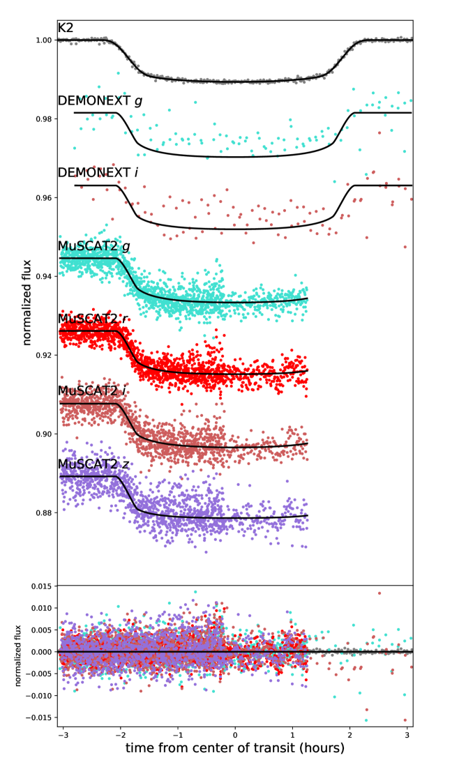
Figure 6: Top: light curves of K2-260, phase-folded on the transit period and with the best-fit transit models overplotted. The transits in each band-instrument combination are offset vertically by an arbitrary amount for clarity; note that the DEMONEXT and MuSCAT2 light curves both contain two individual transits overplotted. Bottom: RV measurements for K2-260 phased to the transit period, with the best-fit model from the circular orbital fit overplotted in black. The RV curves corresponding to 50 random draws from the posterior distributions are overplotted in grey. The error bars incorporate both the internal RV errors and the best-fit RV jitter.

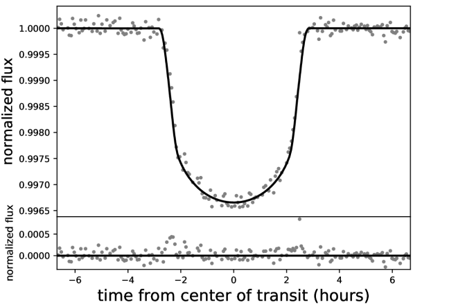
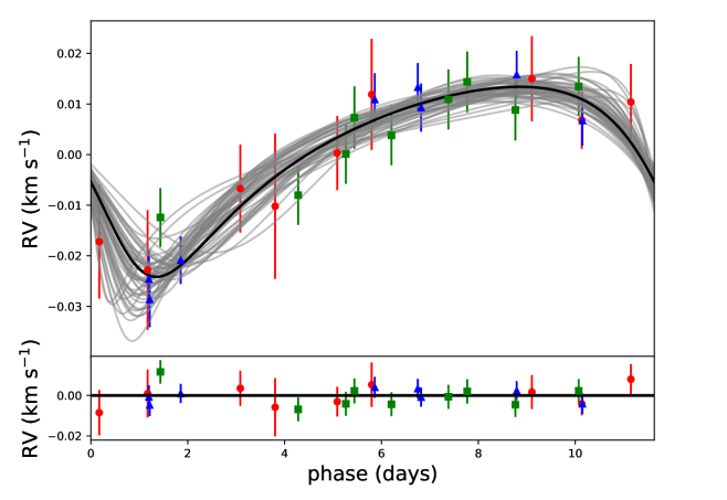
Figure 7: Top: K2 light curve of K2-261, phase-folded on the transit period and with the best-fit transit model overplotted. Bottom: RV measurements of K2-261 from FIES (circles, coloured red online), HARPS-N (triangles, blue online), and HARPS (squares, green online), phased to the transit period and with the best-fit RV model overplotted in black, along with the models corresponding to 50 random draws from the posterior distributions in grey. The error bars incorporate both the internal RV errors and the best-fit RV jitter.

Table 5: Planetary parameters of K2-260 b and K2-261 b

Parameter (unit)	K2-260 b	K2-260 b	K2-261 b	K2-261 b
	circular fit	eccentric fit	circular fit	eccentric fit
	(preferred)			(preferred)
$\Delta$ BIC (circular $-$ eccentric)	$-17.5$		$9.3$
MCMC Parameters
$P$ (days)	$2.6266657\pm 0.0000018$	$2.6266657^{+0.0000020}_{-0.0000018}$	$11.63344\pm 0.00012$	$11.63344\pm 0.00012$
$T_{0}$ (BJD)	$2457820.738135\pm 0.000090$	$2457820.738133^{+0.000091}_{-0.000098}$	$2457906.84115\pm 0.00045$	$2457906.84084^{+0.00054}_{-0.00067}$
$R_{P}/R_{\star}$	$0.09731^{+0.00032}_{-0.00025}$	$0.09731^{+0.00033}_{-0.00027}$	$0.05281^{+0.00104}_{-0.00051}$	$0.05293^{+0.00096}_{-0.00051}$
$a/R_{\star}$	$5.291^{+0.033}_{-0.073}$	$5.34^{+0.92}_{-1.00}$	$17.79^{+0.57}_{-1.00}$	$13.3^{+2.4}_{-2.6}$
$b$	$0.122^{+0.090}_{-0.082}$	$0.116^{+0.096}_{-0.083}$	$0.27^{+0.19}_{-0.18}$	$0.27\pm 0.18$
$e\sin\omega$	0 (fixed)	$-0.02^{+0.21}_{-0.17}$	0 (fixed)	$0.22^{+0.16}_{-0.13}$
$e\cos\omega$	0 (fixed)	$-0.0025^{+0.0042}_{-0.0040}$	0 (fixed)	$-0.29^{+0.12}_{-0.11}$
$K$ (km s-1)	$0.178^{+0.038}_{-0.039}$	$0.174^{+0.040}_{-0.041}$	$0.0137^{+0.0023}_{-0.0021}$	$0.0188\pm 0.0026$
$\gamma_{\mathrm{FIES}}$ (km s-1)	$29.070\pm 0.025$	$29.067^{+0.026}_{-0.027}$	$-0.0137\pm 0.0032$	$-0.0147^{+0.0032}_{-0.0031}$
$\gamma_{\mathrm{HARPS-N}}$ (km s-1)			$3.3323\pm 0.0044$	$3.3356^{+0.0018}_{-0.0024}$
$\gamma_{\mathrm{HARPS}}$ (km s-1)			$3.3428\pm 0.0017$	$3.3411^{+0.0021}_{-0.0023}$
jitterFIES (km s-1)	$0.027^{+0.030}_{-0.019}$	$0.028^{+0.029}_{-0.019}$	$0.0042^{+0.0047}_{-0.0029}$	$0.0032^{+0.0037}_{-0.0022}$
jitterHARPS-N (km s-1)			$0.0121^{+0.0054}_{-0.0033}$	$0.0046^{+0.0034}_{-0.0021}$
jitterHARPS (km s-1)			$0.0045^{+0.0020}_{-0.0013}$	$0.0057^{+0.0027}_{-0.0019}$
Derived Parameters
$\delta$ (%)	$0.9470^{+0.0062}_{-0.0048}$	$0.9470^{+0.0064}_{-0.0053}$	$0.2789^{+0.0111}_{-0.0054}$	$0.2801^{+0.0102}_{-0.0054}$
$i$ (∘)	$88.67^{+0.89}_{-1.00}$	$88.76^{+0.86}_{-1.00}$	$89.15^{+0.58}_{-0.75}$	$88.4^{+1.1}_{-1.9}$
$\rho_{\star}$ ($\rho_{\odot}$)	$0.2881^{+0.0054}_{-0.0100}$	$0.33^{+0.60}_{-0.23}$	$0.558^{+0.055}_{-0.100}$	$0.100^{+0.160}_{-0.073}$
$T_{14}$ (days)	$0.17365^{+0.00045}_{-0.00040}$	$0.171^{+0.041}_{-0.026}$	$0.2124^{+0.0018}_{-0.0014}$	$0.213^{+0.057}_{-0.029}$
$T_{23}$ (days)	$0.14196^{+0.00049}_{-0.00073}$	$0.140^{+0.033}_{-0.021}$	$0.1891^{+0.0015}_{-0.0027}$	$0.189^{+0.051}_{-0.025}$
$T_{\mathrm{peri}}$ (BJD)	$2457820.738135\pm 0.000090$	$2457820.757^{+1.281}_{-0.050}$	$2457906.84115\pm 0.00045$	$2457907.58^{+0.59}_{-0.40}$
$e$	0 (fixed)	$0.134^{+0.124}_{-0.092}$	0 (fixed)	$0.39\pm 0.15$
$\omega$ (∘)	90 (fixed)	$262.0^{+7.9}_{-170.0}$	90 (fixed)	$143.0\pm 18.0$
$a$ (AU)	$0.0404^{+0.0013}_{-0.0016}$	$0.0407^{+0.0071}_{-0.0078}$	$0.1365^{+0.0055}_{-0.0100}$	$0.102^{+0.019}_{-0.020}$
$R_{P}$ ($R_{J}$)	$1.552^{+0.048}_{-0.057}$	$1.552^{+0.048}_{-0.057}$	$0.848^{+0.026}_{-0.022}$	$0.850^{+0.026}_{-0.022}$
$M_{P}$ ($M_{J}$)	$1.42^{+0.31}_{-0.32}$	$1.39^{+0.32}_{-0.34}$	$0.163^{+0.028}_{-0.025}$	$0.223\pm 0.031$
$M_{P}\sin i$ ($M_{J}$)	$1.42^{+0.31}_{-0.32}$	$1.39^{+0.32}_{-0.34}$	$0.163^{+0.028}_{-0.025}$	$0.223\pm 0.031$
$M_{P}/M_{\star}$	$0.00107\pm 0.00025$	$0.00104^{+0.00026}_{-0.00027}$	$0.000141^{+0.000024}_{-0.000022}$	$0.000194\pm 0.000027$
$\log g_{P}$ (cgs)	$3.164^{+0.091}_{-0.100}$	$3.154^{+0.095}_{-0.100}$	$2.750^{+0.071}_{-0.079}$	$2.884^{+0.059}_{-0.072}$
$\rho_{P}$ (g cm-3)	$0.50\pm 0.12$	$0.49\pm 0.13$	$0.355^{+0.067}_{-0.064}$	$0.483^{+0.076}_{-0.081}$
$T_{\mathrm{eq}}$ (K)	$1957^{+78}_{-77}$	$1950^{+200}_{-190}$	$928^{+37}_{-19}$	$1080^{+110}_{-100}$
$H$ (km)	$550\pm 130$	$560\pm 150$	$680\pm 120$	$580^{+110}_{-100}$
$2H/R_{P}$	$0.0102\pm 0.0024$	$0.0104^{+0.0028}_{-0.0027}$	$0.0230^{+0.0040}_{-0.0042}$	$0.0195^{+0.0036}_{-0.0034}$
Notes: in the case of circular orbits the epoch of periastron $T_{\mathrm{peri}}$ is identical to the transit epoch as we fix $\omega=90^{\circ}$. The atmospheric scale height $H$ assumes a hydrogen-dominated atmosphere (i.e., a mean molecular weight of 2), and the quantity $2H/R_{P}$ is the fractional surface area of the planetary disk subtended by an atmosphere of thickness $H$.

3.4 Stellar rotation and inclination

Stellar variability with a quasi-sinusoidal shape is easily visible in the K2 light curve of K2-260 (Fig. 1). The period of the variations, approximately 2 days, is too long to be due to $\delta$ Sct pulsations, and $\gamma$ Dor pulsators tend to be hotter than K2-260 is (see e.g. Uytterhoeven et al., 2011). This may therefore be rotational variability. We performed a Fourier analysis of the light curve, finding that the most dominant frequency is at 0.462 cycles day^-1 ($P=2.16$ days); the first harmonic at 0.92 cycles day^-1 ($P=1.08$ days) is also present. This frequency structure is what would be expected for rotation with a period near 2 days; pulsations would result in a different frequency structure. We cannot, however, exclude the possibility that the 2-day peak could in fact be a harmonic, and that the actual rotation period could be an integer multiple of this. We will discuss this possibility in more detail below. There are also several strong peaks with periods of ten to several tens of days, which could be due to evolution of the spot pattern, but a detailed frequency analysis is beyond the scope of this paper.

We measured the details of the 2-day peak using two different methodologies: a Lomb-Scargle periodogram analysis (Lomb, 1976; Scargle, 1982; Zechmeister & Kürster, 2009), and an autocorrelation function analysis (McQuillan et al., 2014). In both cases we estimated the uncertainty on the period using the FWHM of the relevant peak. From the periodogram analysis we found a period of $2.169\pm 0.048$ days, and from the autocorrelation function $2.16\pm 0.49$ days. Both values are consistent but we conservatively adopt the less-certain autocorrelation value.

As mentioned above, while the 2.16-day period may be the rotation period of K2-260, we cannot exclude the possibility that the rotation period may in fact be an integer multiple of this value. In Table 6 we list the rotation period, expected equatorial rotation velocity, implied value of $\sin i_{\star}$, and 1$\sigma$ allowed range of $i_{\star}$ assuming that the true rotation period is 1, 2, 3, or 4 times the 2.16-day period from the light curve.

Several points of interest are revealed by this analysis. First, if the rotation period is in fact 2.16 days, the predicted equatorial rotational velocity is $39.6\pm 9.0$ $\rm km\ s^{-1}$, more than twice the measured $v\sin{i_{\star}}$ of $16.0\pm 2.0$ $\rm km\ s^{-1}$. This would require that the rotation axis of K2-260 be significantly inclined with respect to the plane of the sky: $i_{\star}=23.8_{-6.4}^{+6.7\circ}$. An equatorial velocity of $40$ $\rm km\ s^{-1}$, however, is much higher than typical for stars with the spectral type of K2-260; stars with $T_{\rm eff}$$\sim 6350$ K typically have $v\sin{i_{\star}}$$<20$ $\rm km\ s^{-1}$ (see e.g. Fig. 4 of Winn et al., 2017). This suggests that it is a priori unlikely that the rotation period of K2-260 is in fact 2.16 days, but this cannot be excluded on the basis of our current data.

If the rotation period of K2-260 is in fact two or three times this (4.32 or 6.5 days), then the expected equatorial velocities are $19.8\pm 4.5$ or $13.2\pm 3.0$ $\rm km\ s^{-1}$, respectively, both of which are consistent to within $1\sigma$ with the measured $v\sin{i_{\star}}$, and are also well within the range of $v\sin{i_{\star}}$ values expected for a star of the spectral type of K2-260. On the other hand, in order to explain the quasi-sinusoidal shape of the light curve on a 2.16-day period with a longer rotation period, the spot distribution on the surface of K2-260 would need to have a near-symmetrical two- or three-spot configuration. In these cases, a large inclination of the stellar rotation axis is not required. Indeed, we are only able to set loose 1$\sigma$ constraints of $i_{\star}>36.8^{\circ}$ and $>63.7^{\circ}$ for these two cases. For the 6.5-day rotation period case we note that this requires $\sin i_{\star}>1$ (we find $\sin i_{\star}=1.22\pm 0.32$), but this is still consistent with 1 to within 1$\sigma$. A rotation period of 4 times 2.16 days or greater would require a value of $\sin i_{\star}$ increasingly larger than 1, excluding such values. These would also require increasingly complex and near-symmetrical multi-polar distributions of spots, which are unlikely.

Table 6: Possible rotation periods of K2-260 and consequences thereof

	$P_{\mathrm{rot}}$	$v_{\mathrm{eq}}$	$\sin i_{\star}$	1$\sigma$ range $i_{\star}$
	(days)	($\rm km\ s^{-1}$)		(∘)
1	$2.16\pm 0.49$	$39.6\pm 9.0$	$0.40\pm 0.10$	$17.4-30.6$
2	$4.32\pm 0.98$	$19.8\pm 4.5$	$0.81\pm 0.21$	$>36.8$
3	$6.5\pm 1.5$	$13.2\pm 3.0$	$1.22\pm 0.32$	$>63.7$
4	$8.6\pm 2.0$	$9.9\pm 2.3$	$1.61\pm 0.43$	none

We therefore conclude that the rotation period of K2-260 is one of 2.16, 4.32, or 6.5 days, but cannot confidently distinguish among these possibilities. We will discuss the implications of these possible rotation periods in more detail in §4.3.

Although sufficient spot coverage to induce measurable rotational modulation is unusual for late F stars, it is not unprecedented; for instance, Mazeh et al. (2015) were able to measure rotation periods for numerous stars in the Kepler field with $T_{\rm eff}$ values as high as 6500 K.

We did not detect any significant rotational modulation in the light curve of K2-261, and so we cannot perform a similar analysis for that star. Based upon our values of $v\sin{i_{\star}}$ and $R_{\star}$ for this object, we calculate a $1\sigma$ upper limit on the expected rotation period of $37.2$ days. The more pole-on K2-261 is viewed, the shorter the rotation period must be to explain the measured $v\sin{i_{\star}}$.

3.5 Secondary eclipse of K2-260

We searched the K2 light curve for a secondary eclipse for K2-260, which, if of large enough magnitude, could have indicated that the system was a false positive. We subtracted the stellar variability of K2-260 by fitting a second-order polynomial to each 0.25$\times P_{\mathrm{orb}}$ portion of the out-of-transit light curve. This aggressive detrending procedure was necessitated by the stellar variability with a period close to the planetary orbital period (2.16 days versus 2.63 days; see §3.4). Although this detrending should have also removed any phase curve which might be present in the K2 light curve, disentangling the phase curve and stellar variability will be very difficult (see §4.4 for further discussion), and so we chose to detrend out both the stellar variability and the phase curve and concentrate on detecting the secondary eclipse. We phase-folded and binned the detrended K2 light curve on the planetary orbital period, which is shown in Fig. 8. We do indeed detect a secondary eclipse.

We fit the eclipse with an occultation model and an MCMC procedure. We obtain a best-fit secondary eclipse depth of $\delta_{\mathrm{sec}}=71\pm 15$ ppm, as well as $e\cos\omega=-0.0049_{-0.0036}^{+0.0048}$. The secondary eclipse depth is small, and is consistent with K2-260 b being a planet (which is also confirmed by our RV measurements). See §4.4 for further discussion.

The value of $e\cos\omega$ that we obtained is consistent with zero to within $1.4\sigma$. We thus conclude that there is no compelling evidence from the secondary eclipse for any orbital eccentricity, nor is there from the radial velocity data (§3.3).

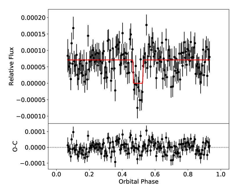
Figure 8: K2 light curve of K2-260 (top), after the stellar variability and in-transit data have been removed and the data have been folded and binned on the orbital period. We show the data in black, and the best-fit secondary eclipse model as a dashed line (red online). The residuals to the fit are shown in the bottom panel.

4 Discussion

4.1 Properties of the planets and systems

In many ways both K2-260 b and K2-261 b are typical representatives of the populations to which they belong. In Fig. 9 we show these two planets in context in the mass-radius diagram.

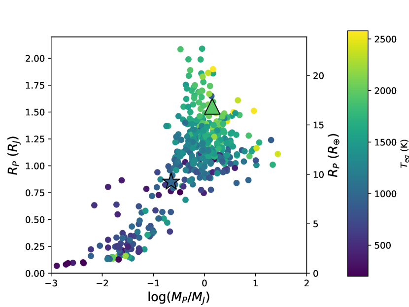
Figure 9: K2-260 b (triangle) and K2-261 b (star) in context with the population of transiting planets with mass and radius measurements, as obtained from the NASA Exoplanet Archive (https://exoplanetarchive.ipac.caltech.edu/) on 2018 March 7. The plot points are coloured according to the zero-albedo equilibrium temperature $T_{\mathrm{eq}}$.

K2-260 b is a fairly typical hot Jupiter of 1.4 $\,M_{\rm J}$ and 1.6 $\,R_{\rm J}$ on a circular 2.6-day orbit. It is slightly inflated, which is expected for its mass and zero-albedo equilibrium temperature of $\sim 2000$ K; planets in this region of the mass-radius diagram tend to have similar equilibrium temperatures (Fig. 9). K2-260 b is most noteworthy in that there is a possibility that its orbit may be misaligned with respect to its host star’s rotation (§4.3), and that it shows a secondary eclipse in the Kepler bandpass (§4.4).

K2-261 b is also exemplary of the population of warm Saturns. Although its radius is somewhat too large to be part of the population of sub-Saturns identified by Petigura et al. (2017)–its radius is 9.2 $\,R_{\oplus}$, while Petigura et al. (2017) defined sub-Saturns as having radii between 4 and 8 $\,R_{\oplus}$–it nonetheless follows many of the same trends seen in this population. For instance, like warm sub-Saturns around metal-rich stars (Petigura et al., 2017), K2-261 b has an eccentric orbit, no additional known planets in the system, and a relatively high mass ($65\,M_{\oplus}$, which is at the upper end of the range typical of sub-Saturns).

K2-261 is also interesting in that it is one of the older planet-host stars with a well-determined age. The NASA Exoplanet Archive lists only eighteen planet-host stars (as of 2017 May 24) with ages of $>8.5$ Gyr and an age uncertainty of less than 2 Gyr. K2-261 is among the most metal-rich of these systems, although its metallicity is not unprecedented for a star of this age (cf. Fig. 10 of Silva Aguirre et al., 2018).

K2-261 b is additionally one of three recently discovered $P\sim 12$ day warm Saturns on eccentric orbits around bright stars from K2, along with K2-232 b (Brahm et al., 2018b; Yu et al., 2018) and K2-234 b (Van Eylen et al., 2018; Yu et al., 2018). Although K2-261 b is somewhat fainter than either of these stars (which have $V=9.3$ and $V=9.9$ respectively), it is nonetheless bright enough to enable many follow-up observations, and will allow comparisons to these other planets. It is intermediate in mass and radius to these two, and the system also has a very similar age to K2-234 (Van Eylen et al., 2018), which will also be helpful for comparative planetology.

4.2 Candidate Stellar Companion to K2-260

As discussed in §2.2, we detected a candidate stellar companion to K2-260 using our Subaru IRCS high-resolution imaging. As can be seen in Fig. 2, the candidate companion is close to the speckle pattern, but we found that it has a contrast of more than $5\sigma$ and is therefore likely to be real.

As we only have a single epoch of single-band imaging, we cannot confirm the association of the candidate companion via the usual methods of common proper motion or colours indicating that it is consistent with being located at the same distance. We therefore must rely upon probabilistic arguments. In order to assess the probability that the candidate companion is indeed physically associated with K2-260, we followed essentially the same methodology as used by Johnson et al. (2018) to estimate the probability that the candidate companion could be a background source. We obtained Galactic models computed by the trilegal (Girardi et al., 2005) and Besançon (Robin et al., 2003) codes for the coordinates of K2-260. We used the default parameters for both codes, except for using the Schlafly & Finkbeiner (2011) reddening maps for trilegal and the Marshall et al. (2006) dust map for Besançon. We then counted the number of sources in each model, and used this to estimate the probability that there would be a background source at least as bright as the candidate companion at least as close to K2-260 as the candidate companion. We found that the probability of such a chance superposition is 0.13% for the trilegal model, and 0.016% for the Besançon model. Although these estimates are in disagreement with each other by about an order of magnitude, we nonetheless conclude that the candidate companion is very likely to be physically associated with the K2-260 system. We caution, however, that we cannot confirm its association with our current data. We proceed for the remainder of the section with further analyses under the assumption that the candidate companion is indeed physically bound to K2-260.

We used the isochrones package (Morton et al., 2016) to estimate what stellar properties of the candidate companion would result in the observed $\Delta H$ value given the properties of the primary. Using the 2MASS $H$-band magnitude and Gaia DR2 parallax, K2-260 has an absolute magnitude of $M_{H}=2.039\pm 0.069$, and the candidate companion therefore has $M_{H}=8.78\pm 0.19$. This corresponds to a mass of $\sim 0.13-0.16$$\,M_{\odot}$ for the candidate companion, taking into account the uncertainties on the age and metallicity of the primary. This would correspond to $T_{\rm eff}$$\sim 3200-3300$ K, or, per Kraus & Hillenbrand (2007), a spectral type of M5-6V.

The candidate companion is too faint to significantly affect our other analyses of this system. Assuming the stellar parameters found earlier, the companion would have a magnitude ratio in the Kepler bandpass of $\Delta Kp\sim 9.5$ (again using isochrones). This would result in a dilution of the transit depth of K2-260 of less than 2 parts in $10^{-5}$, which is much smaller than the uncertainty on the transit depth due to the photometric noise in the light curve, and is thus negligible. Similarly, the companion is too faint to be an eclipsing binary causing the transits of K2-260; in order to cause a transit of the observed depth, even a 100 per cent deep eclipse would need to occur on a companion no fainter than $\Delta Kp\sim 5.1$. This possibility is also excluded by our detection of the reflex motion of K2-260 due to the planet, and the achromaticity of the transit in our MuSCAT2 data.

The discovery of a candidate stellar companion to K2-260 is scientifically interesting for a number of reasons. Ngo et al. (2016) found that host stars of hot Jupiters are significantly more likely than field stars to host stellar companions between 50 and 2000 AU, which tend to have mass ratios smaller than would be expected given the population of field binaries. The candidate companion to K2-260 fits this trend, with its projected separation of 400 AU and mass ratio of $\sim 0.1$, and is furthermore close and massive enough to likely be able to drive planetary migration via Kozai-Lidov oscillations (e.g., Fabrycky & Tremaine, 2007; Naoz et al., 2012) We therefore encourage additional observations of K2-260 to confirm whether the candidate companion is bound to the system.

4.3 Orbital alignment of K2-260 b

Based upon the rotational variability in the light curve of K2-260 (§3.4), we found that the rotation axis of K2-260 may be significantly inclined with respect to the plane of the sky, depending upon whether the true rotation period is 2.16 days or an integer multiple thereof. This has consequences for the orbit of the planet. If the stellar rotation axis is inclined with respect to the plane of the sky, then the planetary orbit must have a substantial obliquity with respect to the stellar spin in order to transit. This would not be unexpected, as K2-260 is above the Kraft break (Kraft, 1967), the point on the main sequence above which stars rotate rapidly due to their lack of a deep surface convective zone, a strong magnetic dynamo, and consequent rotational braking. Hot Jupiters around stars above the Kraft break often have substantially misaligned orbits (Winn et al., 2010; Albrecht et al., 2012). If instead the rotation period is twice or three times 2.16 days, a large stellar inclination, and therefore a misaligned orbit, are not required. This does not, however, exclude the possibility of a misaligned orbit; even if the stellar rotation axis is perpendicular to the line of sight, the sky-projected spin-orbit misalignment $\lambda$ can be large. We cannot constrain $\lambda$ with our current data, but this could easily be measured using the Rossiter-McLaughlin effect (§4.5).

We also note that if the rotation period is in fact 2.16 days, this is close to the 2.63-day planetary orbital period. Systems with $P_{\mathrm{orb}}\sim P_{\mathrm{rot}}$ have different tidal dynamics from those with rotation periods much different from the orbital period, including likely enhanced tidal dissipation (e.g., Collier Cameron & Jardine, 2018), and therefore K2-260 may be of interest from this standpoint. As also discussed by Collier Cameron & Jardine (2018), the dissipation is likely different for spin-orbit misaligned systems near the stellar rotation period due to the different motion of the tidal bulge, providing additional motivation to measure the Rossiter-McLaughlin effect for K2-260 (§4.5). In addition, K2-260 may join a number of F stars with hot Jupiters where the stellar rotation is quasi-synchronized to the planetary orbit, such as $\tau$ Boo (Donati et al., 2008) and CoRoT-4 (Lanza et al., 2009). Such systems were predicted to be an effective end-point of hot Jupiter tidal evolution for F stars by Damiani & Lanza (2015), as reduced tidal damping when $P_{\mathrm{rot}}\sim P_{\mathrm{orb}}$ will delay the planet reaching the point where it can be tidally disrupted. K2-260’s relatively advanced age for an F star, near the main-sequence turn-off, is consistent with this picture; the system has had ample time to evolve into such a quais-stable state. On the other hand, Collier Cameron & Jardine (2018) found evidence of stronger tidal damping for (aligned) systems with $P_{\mathrm{rot}}\sim P_{\mathrm{orb}}$. K2-260 could thus offer an opportunity to test the impact of any spin-orbit misalignment upon this evolution.

4.4 Secondary eclipse of K2-260 b

K2-260 b is one of a relatively small number of planets with a significantly detected secondary eclipse in the Kepler bandpass, and the first such hot Jupiter discovered using K2 (although K2-113 b has a $1.9\sigma$ detection of the secondary eclipse, and the ultra short period planet K2-141 b also has a detected secondary eclipse: Espinoza et al., 2017; Malavolta et al., 2018).

From Esteves et al. (2013), the secondary eclipse depth in the Kepler bandpass is

$$\delta_{\mathrm{sec}}=\bigg{(}\frac{R_{P}}{R_{\star}}\bigg{)}^{2}\frac{\int B_{\lambda}(T_{B})T_{K}d\lambda}{\int F_{\lambda}T_{K}d\lambda}+A_{g}\bigg{(}\frac{R_{P}}{R_{\star}}\frac{R_{\star}}{a}\bigg{)}^{2}$$ (1)

where $B_{\lambda}$ is the Planck function, $T_{B}$ is the blackbody temperature of the planetary dayside, $T_{K}$ is the Kepler bandpass transmission function, $F_{\lambda}$ is the stellar flux, and $A_{g}$ is the planetary geometric albedo. This is Eqn. 18 of Esteves et al. (2013), slightly rewritten to accommodate the notation and measured quantities in this article. The first term on the right hand side of Eqn. 1 describes the thermal emission in the Kepler bandpass, while the second term is the contribution of reflected starlight.

We numerically solve this equation for the geometric albedo $A_{g}$, assuming, after Esteves et al. (2013), that $T_{B}=T_{\mathrm{eq}}(A_{B})$, where $A_{B}=3/2A_{g}$ is the Bond albedo, and $T_{\mathrm{eq}}=T_{\rm eff}\sqrt{fR_{\star}/a}(1-A_{B})^{1/4}$, where $f$ describes the efficiency of heat redistribution. We used two different limiting cases: homogeneous re-distribution of heat ($f=1/4$) and instant re-radiation from the dayside ($f=2/3$). We also make the simplifying assumptions that the planetary emission and stellar flux are both blackbodies, and that the Kepler bandpass is a tophat function between 4000 Å and 9000 Å (following Huber et al., 2017). In both heat redistribution cases the eclipse depth requires a geometric albedo of $A_{g}\sim 0.2$, and the contribution of thermal emission in the Kepler bandpass is small. Although this estimate is not likely to be completely accurate due to the approximations that we have made, it nonetheless suggests that K2-260 b is likely among the class of more reflective hot Jupiters (e.g., Heng & Demory, 2013; Sheets & Deming, 2017).

The detection of a secondary eclipse that is dominated by reflected starlight also implies that there should in principle be a detectable phase curve in the optical. Our aggressive detrending procedure (§3.5) should have removed the phase curve from our phase-folded light curve, and indeed no phase variation is visible in Fig. 8. The detection of the phase curve, however, would be difficult, as it would require careful detrending of the stellar variability. This would be particularly complicated as the 2.16-day period that dominates the stellar variability (§3.4) is similar to the 2.63-day orbital period (which is why we used an aggressive detrending procedure in the first place). Such a detailed search for the phase curve is beyond the scope of the present work.

4.5 Potential for further observations

Both K2-260 b and K2-261 b are promising targets for future observations to further characterize these systems. As discussed in §4.3, it is possible that K2-260 b has an orbit misaligned with respect to the stellar spin axis. Measuring the sky-projected component of this misalignment ($\lambda$) should be straightforward with either Rossiter-McLaughlin (e.g., Triaud et al., 2010) or Doppler tomographic (e.g., Johnson et al., 2017) observations. Given the properties of this system, we predict a Rossiter-McLaughlin semi-amplitude of $\sim 150$ $\rm m\ s^{-1}$ for K2-260 b using the formulae of Gaudi & Winn (2007). K2-261 b is also a promising target for such observations, with a predicted Rossiter-McLaughlin amplitude of $\sim 7.5$ $\rm m\ s^{-1}$. Furthermore, the transit duration is relatively short for a long-period planet ($\sim 5$ hours), allowing a full transit to be observed in a single night, which is critical for RV Rossiter-McLaughlin observations. K2-260 b and K2-261 b are among the better K2 targets for such observations; indeed, K2-260 b has the highest expected Rossiter-McLaughlin amplitude of any confirmed or validated K2 planet orbiting a star brighter than $V=15$. We show these objects’ expected Rossiter-McLaughlin amplitudes in context with the remainder of the K2 planet population in Fig. 10. These will require the use of large telescopes. As can be seen in Table 3, for K2-260 with FIES we are only able to obtain an RV precision of $\sim 60-150$ $\rm m\ s^{-1}$with 1-hour exposures, which is insufficient to properly resolve the Rossiter-McLaughlin effect; ideally one would need at least 8-10 exposures over the 4-hour transit duration. For K2-261 we are able to obtain a per-point uncertainty of $\sim 1-3$ $\rm m\ s^{-1}$with $\sim 1200-1800$ s exposures with HARPS or HARPS-N, which should be adequate to detect the Rossiter-McLaughlin effect; again, with FIES we are only able to obtain a per-point precision of $\sim 10$ $\rm m\ s^{-1}$ with 3600-second exposures, insufficient to detect the Rossiter-McLaughlin effect for this target.

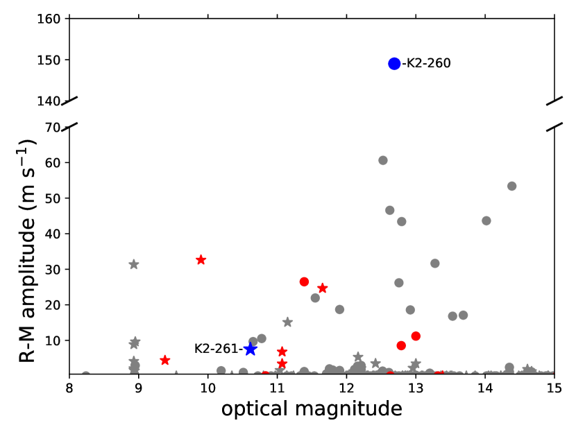
Figure 10: Predicted Rossiter-McLaughlin amplitude as a function of optical magnitude (either $V$ or $Kp$ depending upon the target) for transiting planets discovered by or observed by K2. Approximately Saturn-sized planets ($0.5$$\,R_{\rm J}$$<R_{P}<0.9$$\,R_{\rm J}$) are highlighted in black (red online), while K2-260 and K2-261 are shown in black (blue online) and are noted on the plot. Planets with $P<10$ days are depicted as circles, while those with $P\geq 10$ days are depicted as stars. K2-261 is among the best Saturns and sub-Saturns, and one of the better long-period planets, for an obliquity measurement due to its combination of relatively large Rossiter-McLaughlin amplitude and bright host star. The axes are broken in order to better show K2-260 along with the rest of the population; no K2 planets in the depicted magnitude range have expected R-M amplitudes between 70 and 140 $\rm m\ s^{-1}$, and so the missing region of the plot is empty.

K2-261 is among the brightest stars to host a transiting giant planet with $P>10$ days, which will facilitate other follow-up observations, in particular atmospheric transmission spectroscopy. Thanks to its relatively high temperature ($T_{\mathrm{eq}}=1080^{+110}_{-100}$ K, assuming zero albedo and neglecting the orbital eccentricity) and low surface gravity ($\log g_{P}=2.884^{+0.059}_{-0.072}$), we estimate a planetary atmospheric scale height of $580^{+110}_{-100}$ km, assuming a hydrogen-dominated atmosphere. For K2-260 b we estimate a scale height of $550\pm 130$ km, similar to K2-261 b as the higher planetary gravity largely offsets the higher equilibrium temperature. Although this is also reasonably favourable for transmission spectroscopy, at $V=12.7$ these observations would be challenging simply because of the relative faintness of the host star.

Long-term RV monitoring of both systems could find or constrain the presence of additional planets in these systems. As discussed in §3.3 we found some evidence for a possible RV trend for K2-261, but rejected this possibility as it shifted the parameters of the transiting planet to imply an unphysical solution. Further observations could determine if there in fact might be another planet in the system, either by uncovering a long-term RV trend or finding an RV periodicity due to a shorter-period planet. Our RV monitoring only spans $\sim 100$ days for K2-260 and $\sim 130$ days for K2-261, insufficient to detect any small, long-term trends.

5 Conclusions

We have presented the discovery, confirmation, and initial characterization of two transiting planets from K2, K2-260 b and K2-261 b.

K2-260 b is a somewhat inflated hot Jupiter on a 2.6-day orbit around a mildly rapidly rotating ($v\sin{i_{\star}}$$=16.0\pm 2.0$ $\rm km\ s^{-1}$) F6V star. We detect the secondary eclipse of the planet in the Kepler bandpass, which we find to be largely due to reflected starlight and use to estimate a planetary geometric albedo of $A_{g}\sim 0.2$. The host star also exhibits rotational modulation in its lightcurve. If the dominant periodicity of 2.16 days is the stellar rotation period then the planetary orbit must be misaligned with respect to the stellar rotation axis, as the predicted equatorial rotational velocity is much larger than the measured $v\sin{i_{\star}}$; if, however, the 2.16 day periodicity is a harmonic of the true rotation period, then no large spin-orbit misalignment is required.

K2-261 b is a warm Saturn on an eccentric ($e=0.39$), 11.6-day orbit around a bright ($V=10.6$), metal-rich ($\left[{\rm Fe}/{\rm H}\right]$$=+0.36$) 8.8 Gyr old G7 star at the main sequence turn-off. The star is most likely a member of the Galactic thin disk, and is among the brightest stars to host a transiting giant planet with a period of greater than 10 days.

K2-260 b and K2-261 b add to the sample of transiting giant planets discovered by K2, and are both promising targets for follow-up observations to further characterize these systems. These could include observations of the Rossiter-McLaughlin effect (indeed, K2-260 b should have the largest Rossiter-McLaughlin amplitude of any planet discovered with K2), atmospheric transmission spectroscopy, and long-term RV monitoring.

During the revision process of this paper we became aware of an independent discovery of K2-261 b by Brahm et al. (2018a). No information about this object, including on analysis and results, were shared between the two teams prior to the submission of either paper.

References

- Albrecht et al. (2012) Albrecht S., et al., 2012, ApJ, 757, 18
- Astropy Collaboration et al. (2013) Astropy Collaboration et al., 2013, A&A, 558, A33
- Baranne et al. (1996) Baranne A., et al., 1996, A&AS, 119, 373
- Blanco-Cuaresma et al. (2014) Blanco-Cuaresma S., Soubiran C., Heiter U., Jofré P., 2014, A&A, 569, A111
- Borucki et al. (2010) Borucki W. J., et al., 2010, Science, 327, 977
- Brahm et al. (2018a) Brahm R., et al., 2018a, preprint, (arXiv:1806.04073)
- Brahm et al. (2018b) Brahm R., et al., 2018b, MNRAS, 477, 2572
- Burke et al. (2015) Burke C. J., et al., 2015, ApJ, 809, 8
- Cabrera et al. (2012) Cabrera J., Csizmadia S., Erikson A., Rauer H., Kirste S., 2012, A&A, 548, A44
- Castelli & Kurucz (2004) Castelli F., Kurucz R. L., 2004, ArXiv Astrophysics e-prints, arXiv:0405087,
- Chib & Jeliazkov (2001) Chib S., Jeliazkov I., 2001, Journal of the American Statistical Association, 96, 270
- Claret (2004) Claret A., 2004, A&A, 428, 1001
- Coşkunoǧlu et al. (2011) Coşkunoǧlu B., et al., 2011, MNRAS, 412, 1237
- Collier Cameron & Jardine (2018) Collier Cameron A., Jardine M., 2018, MNRAS, 476, 2542
- Cosentino et al. (2012) Cosentino R., et al., 2012, in Ground-based and Airborne Instrumentation for Astronomy IV. p. 84461V, doi:10.1117/12.925738
- Cutri et al. (2013) Cutri R. M., et al., 2013, VizieR Online Data Catalog, 2328
- Dai et al. (2016) Dai F., et al., 2016, ApJ, 823, 115
- Dai et al. (2017) Dai F., et al., 2017, AJ, 154, 226
- Damiani & Lanza (2015) Damiani C., Lanza A. F., 2015, A&A, 574, A39
- Donati et al. (2008) Donati J. F., et al., 2008, MNRAS, 385, 1179
- Doyle et al. (2014) Doyle A. P., Davies G. R., Smalley B., Chaplin W. J., Elsworth Y., 2014, MNRAS, 444, 3592
- Endl & Cochran (2016) Endl M., Cochran W. D., 2016, PASP, 128, 094502
- Espinoza et al. (2017) Espinoza N., et al., 2017, MNRAS, 471, 4374
- Esteves et al. (2013) Esteves L. J., De Mooij E. J. W., Jayawardhana R., 2013, ApJ, 772, 51
- Fabrycky & Tremaine (2007) Fabrycky D., Tremaine S., 2007, ApJ, 669, 1298
- Foreman-Mackey et al. (2013) Foreman-Mackey D., Hogg D. W., Lang D., Goodman J., 2013, PASP, 125, 306
- Frandsen & Lindberg (1999) Frandsen S., Lindberg B., 1999, in Karttunen H., Piirola V., eds, Astrophysics with the NOT. p. 71
- Fulton et al. (2018) Fulton B. J., Petigura E. A., Blunt S., Sinukoff E., 2018, PASP, 130, 044504
- Gaia Collaboration et al. (2016) Gaia Collaboration et al., 2016, A&A, 595, A1
- Gaia Collaboration et al. (2018) Gaia Collaboration et al., 2018, preprint, (arXiv:1804.09365)
- Gandolfi et al. (2015) Gandolfi D., et al., 2015, A&A, 576, A11
- Gandolfi et al. (2017) Gandolfi D., et al., 2017, AJ, 154, 123
- Gaudi & Winn (2007) Gaudi B. S., Winn J. N., 2007, ApJ, 655, 550
- Girardi et al. (2005) Girardi L., Groenewegen M. A. T., Hatziminaoglou E., da Costa L., 2005, A&A, 436, 895
- Green et al. (2018) Green G. M., et al., 2018, MNRAS, 478, 651
- Grziwa & Pätzold (2016) Grziwa S., Pätzold M., 2016, preprint, (arXiv:1607.08417)
- Grziwa et al. (2012) Grziwa S., Pätzold M., Carone L., 2012, MNRAS, 420, 1045
- Grziwa et al. (2016) Grziwa S., et al., 2016, AJ, 152, 132
- Hartig et al. (2017) Hartig F., Minunno F., Paul S., 2017, BayesianTools: General-Purpose MCMC and SMC Samplers and Tools for Bayesian Statistics. https://github.com/florianhartig/BayesianTools
- Hayano et al. (2010) Hayano Y., et al., 2010, in Adaptive Optics Systems II. p. 77360N, doi:10.1117/12.857567
- Heng & Demory (2013) Heng K., Demory B.-O., 2013, ApJ, 777, 100
- Hirano et al. (2016a) Hirano T., et al., 2016a, ApJ, 820, 41
- Hirano et al. (2016b) Hirano T., et al., 2016b, ApJ, 825, 53
- Howell et al. (2014) Howell S. B., et al., 2014, PASP, 126, 398
- Huber et al. (2016) Huber D., et al., 2016, ApJS, 224, 2
- Huber et al. (2017) Huber K. F., Czesla S., Schmitt J. H. M. M., 2017, A&A, 597, A113
- Jódar et al. (2013) Jódar E., Pérez-Garrido A., Díaz-Sánchez A., Villó I., Rebolo R., Pérez-Prieto J. A., 2013, MNRAS, 429, 859
- Johnson & Soderblom (1987) Johnson D. R. H., Soderblom D. R., 1987, AJ, 93, 864
- Johnson et al. (2016) Johnson M. C., et al., 2016, AJ, 151, 171
- Johnson et al. (2017) Johnson M. C., Cochran W. D., Addison B. C., Tinney C. G., Wright D. J., 2017, AJ, 154, 137
- Johnson et al. (2018) Johnson M. C., et al., 2018, AJ, 155, 100
- Kipping (2013) Kipping D. M., 2013, MNRAS, 435, 2152
- Kobayashi et al. (2000) Kobayashi N., et al., 2000, in Iye M., Moorwood A. F., eds, Proc. SPIEVol. 4008, Optical and IR Telescope Instrumentation and Detectors. pp 1056–1066, doi:10.1117/12.395423
- Kovács et al. (2002) Kovács G., Zucker S., Mazeh T., 2002, A&A, 391, 369
- Kraft (1967) Kraft R. P., 1967, ApJ, 150, 551
- Kraus & Hillenbrand (2007) Kraus A. L., Hillenbrand L. A., 2007, AJ, 134, 2340
- Kreidberg (2015) Kreidberg L., 2015, PASP, 127, 1161
- Labadie et al. (2010) Labadie L., et al., 2010, in Ground-based and Airborne Instrumentation for Astronomy III. p. 77350X (arXiv:1009.4710), doi:10.1117/12.857998
- Lanza et al. (2009) Lanza A. F., et al., 2009, A&A, 506, 255
- Lomb (1976) Lomb N. R., 1976, Ap&SS, 39, 447
- Malavolta et al. (2018) Malavolta L., et al., 2018, AJ, 155, 107
- Marshall et al. (2006) Marshall D. J., Robin A. C., Reylé C., Schultheis M., Picaud S., 2006, A&A, 453, 635
- Mayo et al. (2018) Mayo A. W., et al., 2018, AJ, 155, 136
- Mayor et al. (2003) Mayor M., et al., 2003, The Messenger, 114, 20
- Mazeh et al. (2015) Mazeh T., Perets H. B., McQuillan A., Goldstein E. S., 2015, ApJ, 801, 3
- McQuillan et al. (2014) McQuillan A., Mazeh T., Aigrain S., 2014, ApJS, 211, 24
- Morton & Johnson (2011) Morton T. D., Johnson J. A., 2011, ApJ, 729, 138
- Morton et al. (2016) Morton T. D., Bryson S. T., Coughlin J. L., et al., 2016, ApJ, 822, 86
- Naoz et al. (2012) Naoz S., Farr W. M., Rasio F. A., 2012, ApJ, 754, L36
- Narita et al. (2017) Narita N., et al., 2017, PASJ, 69, 29
- Narita et al. (2018) Narita N., et al., 2018, preprint, (arXiv:1807.01908)
- Ngo et al. (2016) Ngo H., et al., 2016, ApJ, 827, 8
- Niraula et al. (2017) Niraula P., et al., 2017, AJ, 154, 266
- Oscoz et al. (2008) Oscoz A., et al., 2008, in Ground-based and Airborne Instrumentation for Astronomy II. p. 701447, doi:10.1117/12.788834
- Pecaut & Mamajek (2013) Pecaut M. J., Mamajek E. E., 2013, ApJS, 208, 9
- Pepe et al. (2002) Pepe F., Mayor M., Galland F., Naef D., Queloz D., Santos N. C., Udry S., Burnet M., 2002, A&A, 388, 632
- Petigura et al. (2017) Petigura E. A., et al., 2017, AJ, 153, 142
- Pietrinferni et al. (2004) Pietrinferni A., Cassisi S., Salaris M., Castelli F., 2004, ApJ, 612, 168
- Reddy et al. (2006) Reddy B. E., Lambert D. L., Allende Prieto C., 2006, MNRAS, 367, 1329
- Ricker et al. (2015) Ricker G. R., et al., 2015, Journal of Astronomical Telescopes, Instruments, and Systems, 1, 014003
- Robin et al. (2003) Robin A. C., Reylé C., Derrière S., Picaud S., 2003, A&A, 409, 523
- Scargle (1982) Scargle J. D., 1982, ApJ, 263, 835
- Schlafly & Finkbeiner (2011) Schlafly E. F., Finkbeiner D. P., 2011, ApJ, 737, 103
- Sheets & Deming (2017) Sheets H. A., Deming D., 2017, AJ, 154, 160
- Silva Aguirre et al. (2015) Silva Aguirre V., et al., 2015, MNRAS, 452, 2127
- Silva Aguirre et al. (2018) Silva Aguirre V., et al., 2018, MNRAS, 475, 5487
- Sing (2010) Sing D. K., 2010, A&A, 510, A21
- Sing et al. (2016) Sing D. K., et al., 2016, Nature, 529, 59
- Smith et al. (2017) Smith A. M. S., et al., 2017, MNRAS, 464, 2708
- Smith et al. (2018) Smith A. M. S., et al., 2018, MNRAS, 474, 5523
- Sneden (1973) Sneden C., 1973, ApJ, 184, 839
- Southworth (2015) Southworth J., 2015, JKTLD: Limb darkening coefficients, Astrophysics Source Code Library (ascl:1511.016)
- Telting et al. (2014) Telting J. H., et al., 2014, Astronomische Nachrichten, 335, 41
- Triaud et al. (2010) Triaud A. H. M. J., et al., 2010, A&A, 524, A25
- Tull et al. (1995) Tull R. G., MacQueen P. J., Sneden C., Lambert D. L., 1995, PASP, 107, 251
- Uytterhoeven et al. (2011) Uytterhoeven K., et al., 2011, A&A, 534, A125
- Van Eylen et al. (2018) Van Eylen V., et al., 2018, MNRAS,
- Vanderburg & Johnson (2014) Vanderburg A., Johnson J. A., 2014, PASP, 126, 948
- Villanueva et al. (2018) Villanueva Jr. S., Gaudi B. S., Pogge R. W., Eastman J. D., Stassun K. G., Trueblood M., Trueblood P., 2018, PASP, 130, 015001
- Winn et al. (2010) Winn J. N., Fabrycky D., Albrecht S., Johnson J. A., 2010, ApJ, 718, L145
- Winn et al. (2017) Winn J. N., et al., 2017, AJ, 154, 270
- Yu et al. (2018) Yu L., et al., 2018, preprint, (arXiv:1803.02858)
- Zechmeister & Kürster (2009) Zechmeister M., Kürster M., 2009, A&A, 496, 577