Uncertain fate of fair sampling in quantum annealing

Abstract

Recently, it was demonstrated both theoretically and experimentally on the D-Wave quantum annealer that transverse-field quantum annealing does not find all ground states with equal probability. In particular, it was proposed that more complex driver Hamiltonians beyond transverse fields might mitigate this shortcoming. Here, we investigate the mechanisms of (un)fair sampling in quantum annealing. While higher-order terms can improve the sampling for selected small problems, we present multiple counterexamples where driver Hamiltonians that go beyond transverse fields do not remove the sampling bias. Using perturbation theory we explain why this is the case. In addition, we present large-scale quantum Monte Carlo simulations for spin glasses with known degeneracy in two space dimensions and demonstrate that the fair-sampling performance of quadratic driver terms is comparable to standard transverse-field drivers. Our results suggest that quantum annealing machines are not well suited for sampling applications, unless post-processing techniques to improve the sampling are applied.

Quantum annealing (QA) Finnila et al. (1994); Kadowaki and Nishimori (1998); Brooke et al. (1999); Farhi et al. (2001); Santoro et al. (2002); Das and Chakrabarti (2005); Santoro and Tosatti (2006); Das and Chakrabarti (2008); Morita and Nishimori (2008) is a heuristic designed to harness the advantages of quantum mechanics to solve optimization problems. The performance of QA and, in particular, QA machines such as the D-Wave Systems Inc. devices are controversial to date Dickson et al. (2013); Pudenz et al. (2014); Smith and Smolin (2013); Boixo et al. (2013); Albash et al. (2015a); Rønnow et al. (2014); Katzgraber et al. (2014); Lanting et al. (2014); Santra et al. (2014); Shin et al. (2014); Vinci et al. (2014); Boixo et al. (2014); Albash et al. (2015b, a); Katzgraber et al. (2015); Martin-Mayor and Hen (2015); Pudenz et al. (2015); Hen et al. (2015); Venturelli et al. (2015); Vinci et al. (2015); Zhu et al. (2016); Mandrà et al. (2016); Mandrà and Katzgraber (2017a, b). Most studies have focused on finding the minimum value of a binary quadratic cost function (problem Hamiltonian), yet less on the variety of solutions obtained when repeating the optimization procedure multiple times. Important applications that rely on sampling, such as satisfiability (SAT)-based probabilistic membership filters Weaver et al. (2014); Schaefer (1978); Douglass et al. (2015); Herr et al. (2017), propositional model counting and related problems Jerrum et al. (1986); Gomes et al. (2008); Gopalan et al. (2011), or machine learning Hinton (2002); Eslami et al. (2014) rely on ideally uncorrelated states. This sought-after fair sampling ability of an algorithm, i.e., the ability to find (ideally all) states associated with a cost function with (ideally) the same probability, is thus of importance for a variety of applications. Moreover, the ability of an algorithm to sample ground states with similar probability is directly related its ergodicity which strongly influences the efficiency of optimization and sampling techniques.

Following small-scale studies Matsuda et al. (2009), Ref. Mandrà et al. (2017) recently performed systematic experiments on the D-Wave 2X annealer. The results demonstrated that quantum annealers using a transverse-field driver are biased samplers, an effect also observed in previous studies Boixo et al. (2013); Albash et al. (2015a); King et al. (2016). Matsuda et al. Matsuda et al. (2009) conjectured that more complex drivers might alleviate this bias, something we test in this Rapid Communication.

Binary optimization problems can be mapped onto $\mathit{k}$-local spin Hamiltonians. Without loss of generality we study problem Hamiltonians with ${\mathit{N}}$ degrees of freedom in a ${\mathbf{z}}$-basis of the form

$${\cal H}_{\rm P}=-\sum_{i,j=1}^{N}J_{ij}\sigma^{\mathbf{z}}_{i}\sigma^{\mathbf{z}}_{j},$$ (1)

where $\sigma_{i}^{\mathbf{z}}$ is the ${\mathbf{z}}$-component of the Pauli operator acting on site $\mathit{i}$. Note that local biases can also act on the variables. For such a problem Hamiltonian, in principle, a driver of the form

$${\cal H}_{{\mathbf{x}},{\mathit{n}}}=\sum_{i=1}^{\mathit{n}}\Gamma^{{\mathbf{x}},i}[\otimes\sigma^{\mathbf{x}}]^{i}$$ (2)

would induce transitions between all states if ${\mathit{n}}$ is set to ${\mathit{N}}$ and therefore ensure a fair sampling, provided the anneal is performed slow enough. Unfortunately, such a driver is hard to engineer and, at best, one can expect drivers of the form ${\cal H}_{{\mathbf{x}},2}=-\sum_{j}\Gamma^{\mathbf{x}}\sigma_{j}^{\mathbf{x}}+\sum_{j,k}K_{j,k}^{\mathbf{x}}\sigma_{j}^{\mathbf{x}}\sigma_{k}^{\mathbf{x}}$. Quantum fluctuations are induced by the driver and then reduced to sample states from the problem Hamiltonian, i.e., ${\cal H}(\mathit{t})=(1-\mathit{t}/\mathit{T}){\cal H}_{{\mathbf{x}},n}+(\mathit{t}/\mathit{T}){\cal H}_{\rm P}$, where $\mathit{t}\in[0,\mathit{T}]$, $T$ the annealing time, and $\mathit{n}$ the order of the interactions in the driver. For an infinitely-slow anneal, the adiabatic theorem Kadowaki and Nishimori (1998); Farhi et al. (2000) ensures that for $\mathit{t}=\mathit{T}$ a (ground) state of the problem Hamiltonian is reached. It is therefore desirable to know if after an infinite amount of repetitions, the process results in all minimizing states, i.e., fair sampling.

Here we analyze the behavior of more complex drivers of the form ${\cal H}_{{\mathbf{x}},n}$ ($\mathit{n}>1$) on the fair sampling abilities of QA. Following Ref. Matsuda et al. (2009) we first study small systems where the Schrödinger equation can be integrated using qutip Johansson et al. (2013). We have exhaustively analyzed all possible graphs with up to ${\mathit{N}}=6$ with both ferromagnetic and antiferromagnetic interactions and show in Fig. 1 paradigmatic examples that illustrate different scenarios using drivers with $\mathit{n}\leq 2$. Even for some of these small instances, in some cases the inclusion of higher-order driver terms does not remove the bias. If we anneal adiabatically, i.e., $\mathit{T}$ large enough, the instantaneous ground states are never left, which means towards the end of annealing at $\mathit{T}-\mathit{\lambda}$ (for a small $\mathit{\lambda}>0$) the system is in the ground state of ${\cal H}(\mathit{T}-\mathit{\lambda})$. This observation is key to predicting the sampling probabilities for different degenerate ground states. These probabilities are given by squaring the amplitudes of the lowest eigenvector of ${{\cal H}(\mathit{T}-\mathit{\lambda})}$, assuming for now the small contribution from the driver lifts the degeneracies. Because ${\cal H}(\mathit{T}-\mathit{\lambda})$ can be viewed as ${\cal H}_{\rm P}$ perturbed by ${\cal H}_{{\mathbf{x}},n}$, we analyze fair sampling using a perturbative approach Lanting et al. (2017). To better quantify the fair-sampling behavior of a given system, we use the term hard suppression (i.e., total suppression) if the sampling probability is $0$ for a particular ground-state configuration at the end of the anneal and the term soft suppression if a particular state is undersampled by a certain finite fraction in comparison to other minimizing configurations. Finally, we complement these studies with quantum Monte Carlo simulations for large two-dimensional Ising spin-glass problems following Ref. Mandrà et al. (2017) and discuss the effects of higher-order drivers. Our results show that QA is not well suited for sampling applications, unless post processing techniques are implemented Ochoa et al. (2018).

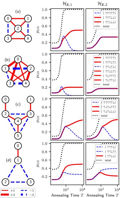
Figure 1: Toy problems with up to ${\mathit{N}}=6$ variables and both ferromagnetic (solid lines) and antiferromagnetic (dashed lines) interactions of different strength (thickness of the lines) integrated using qutip Johansson et al. (2013). Data for both transverse field (${\cal H}_{{\mathbf{x}},1}$) and quadratic (${\cal H}_{{\mathbf{x}},2}$) drivers are shown. The data show the instantaneous probability ${\mathit{p}}_{\rm GS}$ to find different states that minimize the cost function (up to spin-reversal symmetry) as a function of anneal time $\mathit{t}$. In all cases, the first spin (labeled with $0$) is in the state $|\uparrow\rangle$. (a) Toy problem studied in Ref. Matsuda et al. (2009) where drivers with ${\mathit{n}}=2$ sample the states fairly. (b) Similar behavior to (a), however, the unfair sampling sets in earlier in the anneal. (c) Even the inclusion of ${\mathit{n}}=2$ drivers does not remove the unfair sampling. As in (a) and (b) at least one state is suppressed. Note that a driver Hamiltonian with ${\mathit{n}}=4$ results in fair sampling. (d) The sampling is not exponentially biased. However, one state occurs twice as likely as the others. Note that the sampling probabilities swap when going from ${\mathit{n}}=1$ to ${\mathit{n}}=2$.

Perturbation theory. In the following, we show how to determine the sampling probabilities, as well as the influence the driver has on it. Similar work has been done in Sieberer and Lechner (2018). In short, if we apply ${\cal H}_{\rm D}$ as a perturbation of strength $\mathit{\lambda}$ to ${\cal H}_{\rm P}$, some degeneracies will be lifted, i.e. the perturbed ground-state space is smaller. The ground-state space is never left during an adiabatic anneal, hence it will not be possible to reach the entire ground-state space of the unperturbed hamiltonian by annealing in the generic case. This analysis hold for any driver hamiltonian ${\cal H}_{\rm D}$, not just the stoquastic ${\cal H}_{{\mathbf{x}},n}$-type drivers we use in this work. In non-degenerate perturbation theory, the first order corrected wave function $|{\mathit{n}}\rangle$ is given by $|{\mathit{n}}\rangle=|{\mathit{n}}^{0}\rangle+\lambda\sum_{{\mathit{m}}\neq{\mathit{n}}}\frac{\langle{\mathit{m}}^{0}|H_{\rm D}|{\mathit{n}}^{0}\rangle}{E_{\mathit{m}}^{0}-E_{\mathit{n}}^{0}}|{\mathit{m}}^{0}\rangle$, where $|{\mathit{n}}^{0}\rangle$ are the eigenstates and $E_{\mathit{n}}^{0}$ the eigenvalues of the unperturbed hamiltonian ${\cal H}_{\rm P}$. If states ${\mathit{m}}\neq{\mathit{n}}$ are degenerate, i.e. $E_{\mathit{m}}^{0}=E_{\mathit{n}}^{0}$, there is a singularity. To avoid it, degenerate perturbation theory is requires linear combinations $|\alpha^{0}\rangle$ which satisfy $\langle\alpha^{0}|H_{\rm D}|\beta^{0}\rangle\sim\delta_{\alpha,\beta}$ in every degenerate subspace. This ensures that the corrected wave function does not diverge due to singularities. We focus on the ground-state subspace, but the procedure is identical for any subspace. Given ${\mathit{k}}$ ground states $|{\mathit{n}}_{\text{gs}}^{0}\rangle$ of ${\cal H}_{\rm P}$ with energy $E_{\text{gs}}^{0}$, we need to form the ${\mathit{k}}\times{\mathit{k}}$ subspace matrix $V_{{\mathit{n}},{\mathit{m}}}=\langle{\mathit{n}}_{\text{gs}}^{0}|H_{\rm D}|{\mathit{m}}_{\text{gs}}^{0}\rangle$; as shown in Fig. 2. Because $H_{\rm D}$ is Hermitian, $V$ is too. Every Hermitian matrix can be diagonalized by a unitary transformation (${\mathit{U}}^{-1}{\mathit{V}}{\mathit{U}}={\mathit{D}}$) and we find the correct linear combinations $|\alpha_{\text{gs}}^{0}\rangle$ in the columns of ${\mathit{U}}$. It satisfies $\langle\alpha_{\text{gs}}^{0}|V|\beta_{\text{gs}}^{0}\rangle\sim\delta_{\alpha,\beta}$ since D is diagonal. The diagonal entries of $D$ are the eigenvalues of $V$ and also the first order energy corrections $E_{\alpha}^{1}$. We need to pick the lowest eigenvalue $E_{\alpha,\text{low}}^{1}$ and find the corrected ground state energy $E_{GS}=E_{\text{GS}}^{0}+E_{\alpha,\text{low}}^{1}$. The corresponding $l$ eigenvectors $|\alpha_{\text{gs}}^{0}\rangle$ will now determine the sampling behavior, since the annealing state will be in their span. The following scenarios can occur:

(i) ${\mathit{l}}=1$: In this case ${\mathit{p}}_{i}=\langle n_{\text{gs}}^{0}|\phi_{\alpha,\text{low}}^{0}\rangle^{2}$, because there is a single state $|\phi_{\alpha,\text{low}}^{0}\rangle$. If sampling is fair, it will remain fair, regardless of how much the higher energy eigenvalues of ${\cal H}_{\rm P}$ change during the adiabatic anneal. If certain states have ${\mathit{p}}_{i}=0$, $|n_{\text{gs}}^{0}\rangle$ will never be available at the end of the anneal.

(ii) $\l>1$: Let $A$ be the $k\times m$ matrix consisting of all $l$ $|\phi_{\alpha,\text{low}}^{0}\rangle$. If there is a vector $x$ such that $Ax=y$ and $y_{i}\cdot y_{i}^{*}=1$ for all $i$, then fair sampling is potentially possible according to first order. If there exists an $i$ such that $y_{i}=0$ for all $x$, then that ground-state is never found. The same argument can be made for biased sampling where there is no suppression but certain states are over-sampled.

(iii) ${\mathit{V}}$ is zero: All eigenvalues $E_{\alpha}^{1}=0$ and the sampling probabilities are determined by second-order perturbation, i.e., the probabilities depend on higher eigenvalues of ${\cal H}_{\rm P}$ (see Fig. 3).

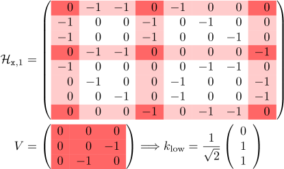
Figure 2: To obtain the sampling probabilities, the ground-state eigenvectors $|g_{i}\rangle$ need to be known, represented here as shaded rows and columns in the matrix ${\cal H}_{\texttt{x},1}$, since the solution of the diagonal ${\cal H}_{\rm P}$ is a classical one. One then needs to analyze the subspace ${\mathit{V}}$ that is formed by restricting the driver (here ${\cal H}_{\texttt{x},1}$) to space spanned by the ground states of ${\cal H}_{\rm P}$. The lowest eigenvector(s) determine the sampling probabilities. In this example, there is one lowest eigenvector and the first ground state corresponding to the top column (first row) is suppressed (all spins up) and will never be sampled in an adiabatic anneal.

The second-order perturbation terms only play a relevant role if ${\mathit{V}}$ is trivial. If $\l>0$, the sampling behavior is determined by ${\mathit{V}}$ which does not depend on ${\cal H}_{\rm P}$. This means that the sampling behavior is purely a property of the driver Hamiltonian ${\cal H}_{{\mathbf{x}},n}$ and the ground-state eigenvectors of ${\cal H}_{\rm P}$. We have verified this on numerous small systems, as well as structured and random-coupling systems with direct integration and were always able to predict the sampling probabilities that correspond to the state found after the anneal.

Figure 1(a) is the example studied in Ref. Matsuda et al. (2009), where ${\cal H}_{{\mathbf{x}},2}$ leads to fair sampling. There are six degenerate ground states, two of which are suppressed. With a driver of the form ${\cal H}_{{\mathbf{x}},1}$ we obtain $\l>1$, meaning that there are multiple $|\alpha_{\text{gs}}^{0}\rangle$ states that determine the sampling. However, the suppressed states have ${\mathit{p}}_{i}=0$. In Fig. 1(b) we show a more complex example – the smallest problem we were able to find that has $\l=1$ and one state where ${\mathit{p}}_{i}=0$. It is a $12$-fold degenerate system with two states fully suppressed when ${\cal H}_{{\mathbf{x}},1}$ is used as a driver. The fact that $\l=1$ could be a reason why the suppression sets in earlier during the anneal. This case is problematic for annealing schedules that are fast quenches, because there is a much smaller window during the anneal where the total ground-state probability is approximately unity and the suppressed state has not yet reached zero probability. Using ${\cal H}_{{\mathbf{x}},2}$ results in fair sampling. Figure 1(c) shows a system that has six ground states with two ground states in hard suppression. Using ${\cal H}_{{\mathbf{x}},1}$ as a driver, we obtain $\l=1$ and a unique $|\alpha_{\text{gs}}^{0}\rangle$ with two hard suppressed states with zero probability. For ${\cal H}_{{\mathbf{x}},2}$, $\l>1$ we obtain multiple $|\alpha_{\text{gs}}^{0}\rangle$ states. However, two states are hard suppressed. Using ${\cal H}_{{\mathbf{x}},3}$ as a driver results in $\l=1$ and a unique $|\alpha_{\text{gs}}^{0}\rangle$. However, there is a soft suppression of two ground states (not shown). Finally, using ${\cal H}_{{\mathbf{x}},4}$ we obtain $\l=1$ and fair sampling. The case shown in Fig. 1(d) reveals the undersampled states when ${\cal H}_{{\mathbf{x}},1}$ is replaced by ${\cal H}_{{\mathbf{x}},2}$. More precisely, it changes from $\l>1$ with four soft suppressed states to $\l=1$ with the previously two oversampled state now being undersampled. Using a driver ${\cal H}_{{\mathbf{x}},3}$ results in $\l=1$ and fair sampling.

Figure 3 shows a problem where by changing the strength of ${\mathit{J}}_{3,4}$ one can change the sampling bias arbitrarily. Note that changing ${\mathit{J}}_{3,4}=-1.2$ to $-1.8$ does shift the relative energies of the ground state and the various low excited states, but does not change their order. In terms of perturbation theory, ${\mathit{V}}$ is trivial, and second-order perturbations dictate the behavior of the system. Because there are terms $\propto 1/(E_{i}-E_{\rm GS})$ with $E_{\rm GS}$ the ground-state energy, shifting the energy levels $E_{i}$ will influence the sampling.

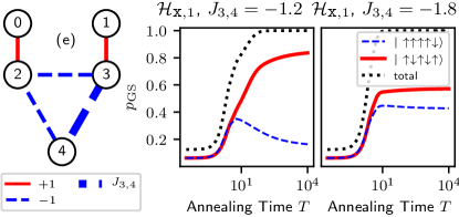
Figure 3: Toy problem with ${\mathit{N}}=5$ variables and both ferromagnetic (solid lines) and antiferromagnetic (dashed lines) interactions of different strength (thickness of the lines) integrated using qutip Johansson et al. (2013). Data for a driver ${\cal H}_{{\mathbf{x}},1}$. By changing $J_{3,4}$ one can change the sampling bias arbitrarily.

Quantum Monte Carlo results. To corroborate our results with larger systems, we perform a fair-sampling study analogous to the one done in Ref. Mandrà et al. (2017) for two-dimensional Ising spin glasses on a square lattice with periodic boundary conditions. The couplers are chosen from ${\mathit{J}}_{i,j}\in\{\pm 1,\pm 2,\pm 4\}$. This ensures that degeneracies are small. The coupler-configuration space is mined for specific degeneracies as done in Ref. Mandrà et al. (2017). Figure 4 shows representative rank-ordered probabilities to find different minimizing configurations using simulated annealing (SA) Kirkpatrick et al. (1983); Isakov et al. (2015); Moreno et al. (2003), as well as transverse-field simulated quantum annealing (SQA-${\cal H}_{{\mathbf{x}},1}$) Santoro et al. (2002); Heim et al. (2015); Isakov et al. (2016); Mazzola et al. (2017); Könz et al. (2018); com (a) and simulated quantum annealing with a stoquastic two-spin driver (SQA-${\cal H}_{{\mathbf{x}},2})$ com (b) Mazzola and Troyer (2017). The data are averaged over $100$ disorder realizations. While the data for SA for this particular problem show a fair sampling of all minimizing configurations, neither a transverse-field ${\cal H}_{{\mathbf{x}},1}$ nor a more complex ${\cal H}_{{\mathbf{x}},2}$ driver can remove the bias. This suggests that even if QA machines with more complex ${\cal H}_{{\mathbf{x}},2}$ drivers are constructed, sampling will remain unfair unless post-processing is applied Ochoa et al. (2018). The close connection between SQA and QA performances is discussed in Refs. Isakov et al. (2016); Mazzola et al. (2017).

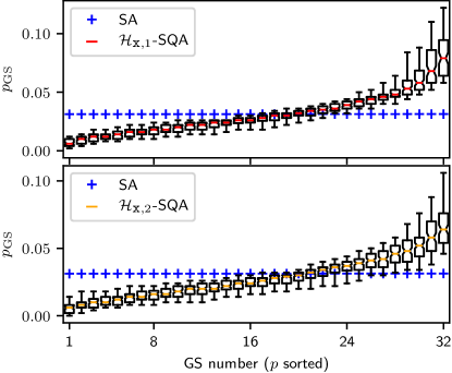
Figure 4: Rank-ordered probability ${\mathit{p}}_{\rm GS}$ to find different degenerate states for a two-dimensional Ising spin glass with ${\mathit{N}}=8^{2}=64$ and a ground-state degeneracy of $32$. The data are averaged over $100$ disorder realizations. For each instances, $500$ independent runs are performed and the probability to find a given ground-state configuration computed. While simulated annealing (SA) samples close to fair, both SQA-${\cal H}_{{\mathbf{x}},1}$ and SQA-${\cal H}_{{\mathbf{x}},2}$ show a clear bias in the sampling. In particular, there is no notable improvement of using a driver of the form ${\cal H}_{{\mathbf{x}},2}$ over a transverse-field driver ${\cal H}_{{\mathbf{x}},1}$. We have also simulated systems with up to ${\mathit{N}}=12^{2}=144$ variables and ground states with up to $96$-fold degeneracy obtaining similar results. Note that the bias becomes more pronounced for increasing system size ${\mathit{N}}$ (not shown).

Effects of more complex drivers. The following section shows that any driver (stoquastic or non-stoquastic) needs to be sufficiently dense to sample fair for generic larger systems. To predict the sampling probabilities it is sufficient to know ${\mathit{V}}$ (except when ${\mathit{V}}$ is trivial). ${\mathit{V}}$ can be constructed with only the ground-state eigenvectors of ${\cal H}_{\rm P}$ (no eigen energies needed) and the driver ${\cal H}_{{\mathbf{x}},n}$. This can be used to analyze different drivers—without specifying a concrete problem Hamiltonian ${\cal H}_{\rm P}$—by merely sampling from possible ground-state combinations. As an example consider a twofold degeneracy in a five-spin system. Because we want to test the driver for all possible ground-state combinations, we can exhaustively generate all the ground-state pairs, i.e., ${\mathit{N}}({\mathit{N}}-1)/2$, where ${\mathit{N}}=2^{5}$ and check ${\mathit{V}}$ for each one pair, to analyze the sampling behavior. For larger $N$, we sample instead of searching exhaustively.

Figure 5 shows how probable it is for a random degeneracy and a ground-state combination to be sampled according to the following categories:

fair: All ground states have the same probability.

soft: At least one ground state is soft suppressed with a ratio smaller than $1:100$ (least likely vs most likely).

hard: At least one ground state is soft suppressed with a ratio larger than $1:100$ or not found at all, i.e., hard suppression. For better visibility in Fig. 5 we combine these two cases. However, most of the time the suppression is hard.

highord: The matrix ${\mathit{V}}$ is trivial. Higher-order perturbation will determine the sampling behavior. In the generic case of random couplings this leads to both soft or hard suppression.

In all cases and for ${\cal H}_{{\mathbf{x}},n}$ with ${\mathit{n}}\leq 8$ we use $\Gamma^{{\mathbf{x}},n}=1$. Using different values for the different amplitudes leads to worse sampling, because the matrix ${\mathit{V}}$ has multiple different entries. A random matrix has a unique eigenvector which is not parallel to $(1,1,\ldots,1,1)$ in the generic case. Hence, introducing more variety into ${\mathit{V}}$ leads to more unique (and unfair) $|\alpha_{\text{gs}}^{0}\rangle$. How the ratio of soft to hard suppression is influenced by this was not investigated, since it is unfair in the generic case. Repeating multiple annealing runs with individually randomized $\Gamma^{{\mathbf{x}},n}_{i,j,...}$ and averaging improves the sampling but, if not dense enough, will not be able to remove all hard suppression in a generic case.

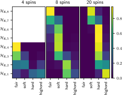
Figure 5: For each spin system all possible degeneracies are sampled with $400$ random ground-state combinations. For small systems, all combinatorial possibilities of ground states can be checked, and the random sampling approximates the exact result fast. For four spins, fair sampling is reached for all possible problem Hamiltonians ${\cal H}_{\rm P}$, once the driver matrix is dense, i.e., all off-diagonal contain nonzero entries,. For example, this is the case when using ${\cal H}_{{\mathbf{x}},4}$ for a system with four spins. Similarly, for eight spins the system moves from hard to soft, to fair sampling as more complex drivers are used. As the system with $20$ spins illustrates, below for any ${\mathit{n}}<7$ in ${\cal H}_{{\mathbf{x}},n}$ there is only a dependence on second-order perturbation (see Fig. 3) or hard suppression in the average case.

Conclusions. We have studied the necessary ingredients needed for quantum annealing to sample ground states fairly. From Fig. 5 we surmise that a fairly dense driver is needed to obtain fair sampling. Carefully controlling the anneal with additional parameters, for example as shown in Ref. Susa et al. (2018) might help mitigate the bias, however, this remains to be tested. We do emphasize, however, that a ${\cal H}_{{\mathbf{x}},2}$ driver with the typical annealing modus operandi used in current hardware will not yield a fair sampling of states and performs comparably to an elementary transverse-field driver ${\cal H}_{{\mathbf{x}},1}$.