The progeny of a Cosmic Titan: a massive multi-component proto-supercluster in formation at z=2.45 in VUDS

We unveil the complex shape of a proto-supercluster at $z\sim 2.45$ in the COSMOS field exploiting the synergy of both spectroscopic and photometric redshifts. Thanks to the spectroscopic redshifts of the VIMOS Ultra-Deep Survey (VUDS), complemented by the zCOSMOS-Deep spectroscopic sample and high-quality photometric redshifts, we compute the three-dimensional (3D) overdensity field in a volume of $\sim 100\times 100\times 250$ comoving Mpc³ in the central region of the COSMOS field, centred at $z\sim 2.45$ along the line of sight. The method relies on a two-dimensional (2D) Voronoi tessellation in overlapping redshift slices that is converted into a 3D density field, where the galaxy distribution in each slice is constructed using a statistical treatment of both spectroscopic and photometric redshifts. In this volume, we identify a proto-supercluster, dubbed “Hyperion” for its immense size and mass, which extends over a volume of $\sim 60\times 60\times 150$ comoving Mpc³ and has an estimated total mass of $\sim 4.8\times 10^{15}{\rm M}_{\odot}$. This immensely complex structure contains at least seven density peaks within $2.4\lesssim z\lesssim 2.5$ connected by filaments that exceed the average density of the volume. We estimate the total mass of the individual peaks, $M_{\rm tot}$, based on their inferred average matter density, and find a range of masses from $\sim 0.1\times 10^{14}{\rm M}_{\odot}$ to $\sim 2.7\times 10^{14}{\rm M}_{\odot}$. By using spectroscopic members of each peak, we obtain the velocity dispersion of the galaxies in the peaks, and then their virial mass $M_{\rm vir}$ (under the strong assumption that they are virialised). The agreement between $M_{\rm vir}$ and $M_{\rm tot}$ is surprisingly good, at less than $1-2\sigma$, considering that (almost all) the peaks are probably not yet virialised. According to the spherical collapse model, these peaks have already started or are about to start collapsing, and they are all predicted to be virialised by redshift $z\sim 0.8-1.6$. We finally perform a careful comparison with the literature, given that smaller components of this proto-supercluster had previously been identified using either heterogeneous galaxy samples (Ly$\alpha$ emitters, sub-mm starbursting galaxies, CO emitting galaxies) or 3D Ly$\alpha$ forest tomography on a smaller area. With VUDS, we obtain, for the first time across the central $\sim 1$ deg² of the COSMOS field, a panoramic view of this large structure, that encompasses, connects, and considerably expands in a homogeneous way on all previous detections of the various sub-components. The characteristics of this exceptional proto-supercluster, its redshift, its richness over a large volume, the clear detection of its sub-components, together with the extensive multi-wavelength imaging and spectroscopy granted by the COSMOS field, provide us the unique possibility to study a rich supercluster in formation.

1 Introduction

Proto-clusters are crucial sites for studying how environment affects galaxy evolution in the early universe, both in observations (see e.g. Steidel et al. 2005; Peter et al. 2007; Miley & De Breuck 2008; Tanaka et al. 2010; Strazzullo et al. 2013) and simulations (e.g. Chiang et al. 2017; Muldrew et al. 2018). Moreover, since proto-clusters mark the early stages of structure formation, they have the potential to provide additional constraints on the already well established probes on standard and non-standard cosmology based on galaxy clusters at low and intermediate redshift (see e.g. Allen et al. 2011; Heneka et al. 2018; Schmidt et al. 2009; Roncarelli et al. 2015, and references therein).

Although the sample of confirmed or candidate proto-clusters is increasing in both number (see e.g. the systematic searches in Diener et al. 2013; Chiang et al. 2014; Franck & McGaugh 2016; Lee et al. 2016; Toshikawa et al. 2018) and maximum redshift (e.g. Higuchi et al. 2018), our knowledge of high-redshift ($z>2$) structures is still limited, as it is broadly based on heterogeneous data sets. These structures span from relaxed to unrelaxed systems, and are detected by using different, and sometimes apparently contradicting, selection criteria. As a non-exhaustive list of examples, high-redshift clusters and proto-clusters have been identified as excesses of either star-forming galaxies (e.g. Steidel et al. 2000; Ouchi et al. 2005; Lemaux et al. 2009; Capak et al. 2011) or red galaxies (e.g. Kodama et al. 2007; Spitler et al. 2012), as excesses of infrared(IR)-luminous galaxies (Gobat et al. 2011), or via SZ signatures (Foley et al. 2011) or diffuse X-ray emission (Fassbender et al. 2011). Other detection methods include the search for photometric redshift overdensities in deep multi-band surveys (Salimbeni et al. 2009; Scoville et al. 2013) or around active galactic nuclei (AGNs) and radio galaxies (Pentericci et al. 2000; Galametz et al. 2012), the identification of large intergalactic medium reservoirs via Ly$\alpha$ forest absorption (Cai et al. 2016; Lee et al. 2016; Cai et al. 2017), and the exploration of narrow redshift slices via narrow band imaging (Venemans et al. 2002; Lee et al. 2014).

The identification and study of proto-structures can be boosted by two factors: 1) the use of spectroscopic redshifts, and 2) the use of unbiased tracers with respect to the underlying galaxy population. On the one hand, the use of spectroscopic redshifts is crucial for a robust identification of the overdensities themselves, for the study of the velocity field, especially in terms of the galaxy velocity dispersion which can be used as a proxy for the total mass, and finally for the identification of possible sub-structures. On the other hand, if such proto-structures are found and mapped by tracers that are representative of the dominant galaxy population at the epoch of interest, we can recover an unbiased view of such environments.

In this context, we used the VUDS (VIMOS Ultra Deep Survey) spectroscopic survey (Le Fèvre et al. 2015) to systematically search for proto-structures. VUDS targeted approximately $10000$ objects presumed to be at high redshift for spectroscopic observations, confirming over $5000$ galaxies at $z>2$. These galaxies generally have stellar masses $\gtrsim 10^{9}{\rm M}_{\odot}$, and are broadly representative in stellar mass, absolute magnitude, and rest-frame colour of all star-forming galaxies (and thus, the vast majority of galaxies) at $2\lesssim z\lesssim 4.5$ for $i\leq 25$. We identified a preliminary sample of $\sim 50$ candidate proto-structures (Lemaux et al, in prep.) over $2<z<4.6$ in the COSMOS, CFHTLS-D1 and ECDFS fields (1 deg² in total). With this ‘blind’ search in the COSMOS field we identified the complex and rich proto-structure at $z\sim 2.5$ presented in this paper.

This proto-structure, extended over a volume of $\sim 60\times 60\times 150$ comoving Mpc³, has a very complex shape, and includes several density peaks within $2.42<z<2.51$, possibly connected by filaments, that are more dense than the average volume density. Smaller components of this proto-structure have already been identified in the literature from heterogeneous galaxy samples, like for example Ly$\alpha$ emitters (LAEs), three-dimensional (3D) Ly$\alpha$-forest tomography, sub-millimetre starbursting galaxies, and CO-emitting galaxies (see Diener et al. 2015; Chiang et al. 2015; Casey et al. 2015; Lee et al. 2016; Wang et al. 2016). Despite the sparseness of previous identifications of sub-clumps, a part of this structure was already dubbed “Colossus” for its extension (Lee et al. 2016).

With VUDS, we obtain a more complete and unbiased panoramic view of this large structure, placing the previous sub-structure detections reported in the literature in the broader context of this extended large-scale structure. The characteristics of this proto-structure, its redshift, its richness over a large volume, the clear detection of its sub-components, the extensive imaging and spectroscopy coverage granted by the COSMOS field, provide us the unique possibility to study a rich supercluster in its formation.

From now on we refer to this huge structure as a ‘proto-supercluster’. On the one hand, throughout the paper we show that it is as extended and as massive as known superclusters at lower redshift. Moreover, it presents a very complex shape, which includes several density peaks embedded in the same large-scale structure, similarly to other lower-redshift structures defined superclusters. In particular, one of the peaks has already been identified in the literature (Wang et al. 2016) as a possibly virialised structure. On the other hand, we also show that the evolutionary status of some of these peaks is compatible with that of overdensity fluctuations which are collapsing and are foreseen to virialise in a few gigayears. For all these reasons, we consider this structure a proto-supercluster.

In this work, we aim to characterise the 3D shape of the proto-supercluster, and in particular to study the properties of its sub-components, for example their average density, volume, total mass, velocity dispersion, and shape. We also perform a thorough comparison of our findings with the previous density peaks detected in the literature on this volume, so as to put them in the broader context of a large-scale structure.

The paper is organised as follows. In Sect. 2 we present our data set and how we reconstruct the overdensity field. The discovery of the proto-supercluster, and its total volume and mass, are discussed in Sect. 3. In Sect. 4 we describe the properties of the highest density peaks embedded in the proto-supercluster (their individual mass, velocity dispersion, etc.) and we compare our findings with the literature. In Sect. 5 we discuss how the peaks would evolve according to the spherical collapse model, and how we can compare the proto-supercluster to similar structures at lower redshifts. Finally, in Sect. 6 we summarise our results.

Except where explicitly stated otherwise, we assume a flat $\Lambda$CDM cosmology with $\Omega_{m}=0.25$, $\Omega_{\Lambda}=0.75$, $H_{0}=70\,{\rm km\,s}^{-1}{\rm Mpc}^{-1}$ and $h=H_{0}/100$. Magnitudes are expressed in the AB system (Oke 1974; Fukugita et al. 1996). Comoving and physical Mpc(/kpc) are expressed as cMpc(/ckpc) and pMpc(/pkpc), respectively.

2 The data sample and the density field

VUDS is a spectroscopic survey performed with VIMOS on the ESO-VLT (Le Fèvre et al. 2003), targeting approximately $10000$ objects in the three fields COSMOS, ECDFS, and VVDS-2h to study galaxy evolution at $2\lesssim z\lesssim 6$. Full details are given in Le Fèvre et al. (2015); here we give only a brief review.

VUDS spectroscopic targets have been pre-selected using four different criteria. The main criterion is a photometric redshift ($z_{p}$) cut ($z_{p}+1\sigma\geq 2.4$, with $z_{p}$ being either the $1^{st}$ or $2^{nd}$ peak of the $z_{p}$ probability distribution function) coupled with the flux limit $i\leq 25$. This main criterion provided 87.7% of the primary sample. Photometric redshifts were derived as described in Ilbert et al. (2013) with the code Le Phare (Arnouts et al. 1999; Ilbert et al. 2006). The remaining targets include galaxies with colours compatible with Lyman-break galaxies, if not already selected by the $z_{p}$ criterion, as well as drop-out galaxies for which a strong break compatible with $z>2$ was identified in the $ugrizYJHK$ photometry. In addition to this primary sample, a purely flux-limited sample with $23\leq i\leq 25$ has been targeted to fill-up the masks of the multi-slit observations.

VUDS spectra have an extended wavelength coverage from 3600 to $9350\AA$, because targets have been observed with both the LRBLUE and LRRED grisms (both with R$\sim 230$), with 14h integration each. With this integration time it is possible to reach S/N $\sim 5$ on the continuum at $\lambda\sim 8500$Å  (for $i=25$), and for an emission line with flux $F=1.5\times 10^{-18}$erg s^-1 cm². The redshift accuracy is $\sigma_{zs}=0.0005(1+z)$, corresponding to $\sim 150\,{\rm km\,s}^{-1}$ (see also Le Fèvre et al. 2013).

We refer the reader to Le Fèvre et al. (2015) for a detailed description of data reduction and redshift measurement. Concerning the reliability of the measured redshifts, here it is important to stress that each measured redshift is given a reliability flag equal to X1, X2, X3, X4, or X9, which correspond to a probability of being correct of 50-75%, 75-85%, 95-100%, 100%, and $\sim 80$% respectively. In the COSMOS field, the VUDS sample comprises 4303 spectra of unique objects, out of which 2045 have secure spectroscopic redshift (flags X2, X3, X4, or X9) and $z\geq 2.$

Together with the VUDS data, we used the zCOSMOS-Bright (Lilly et al. 2007, 2009) and zCOSMOS-Deep (Lilly et al, in prep., Diener et al. 2013) spectroscopic samples. The flag system for the robustness of the redshift measurement is basically the same as in the VUDS sample, with very similar flag probabilities (although they have never been fully assessed for zCOSMOS-Deep). In the zCOSMOS samples, the spectroscopic flags have also been given a decimal digit to represent the level of agreement of the spectroscopic redshift ($z_{s}$) with the photometric redshift ($z_{p}$). A given $z_{p}$ is defined to be in agreement with its corresponding $z_{s}$ when $|z_{s}-z_{p}|<0.08(1+z_{s})$, and in these cases the decimal digit of the spectroscopic flag is ‘5’. For the zCOSMOS samples, we define secure $z_{s}$ those with a quality flag X2.5, X3, X4, or X9, which means that for flag X2 we used only the $z_{s}$ in agreement with their respective $z_{p}$, while for higher flags we trust the $z_{s}$ irrespectively of the agreement with their $z_{p}$. With these flag limits, we are left with more than 19000 secure $z_{s}$, of which 1848 are at $z\geq 2$. We merged the VUDS and zCOSMOS samples, removing the duplicates between the two surveys as follows. For each duplicate, that is, objects observed in both VUDS and zCOSMOS, we retained the redshift with the most secure quality flag, which in the vast majority of cases was the one from VUDS. In case of equal flags, we retained the VUDS spectroscopic redshift. Our final VUDS$+$zCOSMOS spectroscopic catalogue consists of 3822 unique secure $z_{s}$ at $z\geq 2$.

We note that we did not use spectroscopic redshifts from any other survey, although other spectroscopic samples in this area are already publicly available in the literature (see e.g. Casey et al. 2015; Chiang et al. 2015; Diener et al. 2015; Wang et al. 2016). These samples are often follow-up of small regions around dense regions, and we did not want to be biased in the identification of already known density peaks. Unless specified otherwise, our spectroscopic sample always refers only to the good quality flags in VUDS and zCOSMOS discussed above. We also did not include public $z_{s}$ from more extensive campaigns, like for example the COSMOS AGN spectroscopic survey (Trump et al. 2009), the MOSDEF survey (Kriek et al. 2015), or the DEIMOS 10K spectroscopic survey (Hasinger et al. 2018).

We matched our spectroscopic catalogue with the photometric COSMOS2015 catalogue (Laigle et al. 2016). The matching was done by selecting the closest source within a matching radius of $0.55^{\prime\prime}$. Objects in the COSMOS2015 have been detected via an ultra-deep $\chi^{2}$ sum of the $YJHK_{s}$ and $z^{++}$ images. $YJHK_{s}$ photometry was obtained by the VIRCAM instrument on the VISTA telescope (UltraVISTA-DR2 survey, McCracken et al. 2012), and the $z^{++}$ data, taken using the Subaru Suprime-Cam, are a (deeper) replacement of the previous $z-$band COSMOS data (Taniguchi et al. 2007, 2015). With this match with the COSMOS2015 catalogue we obtained a uniform target coverage of the COSMOS field down to a given flux limit (see Sect.3.1), using spectroscopic redshifts for the objects in our original spectroscopic sample or photometric redshifts for the remaining sources. The photometric redshifts in COSMOS2015 are derived using $3^{\prime\prime}$ aperture fluxes in the 30 photometric bands of COSMOS2015. According to Table 5 of Laigle et al. (2016), a direct comparison of their photometric redshifts with the spectroscopic redshifts of the entire VUDS survey in the COSMOS field (median redshift $z_{\rm med}=2.70$ and median $i^{+}-$band $i^{+}_{\rm med}=24.6$) gives a photometric redshift accuracy of $\Delta z=0.028(1+z)$. The same comparison with the zCOSMOS-Deep sample (median redshift $z_{\rm med}=2.11$ and median $i^{+}-$band $i^{+}_{\rm med}=23.8$) gives $\Delta z=0.032(1+z)$.

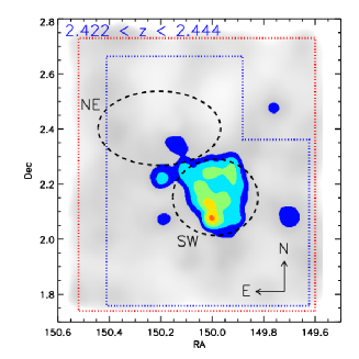
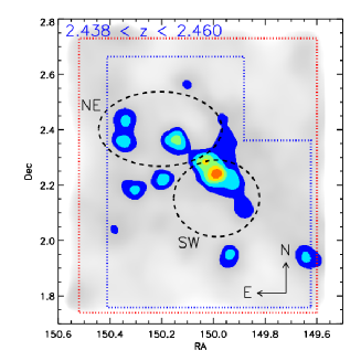
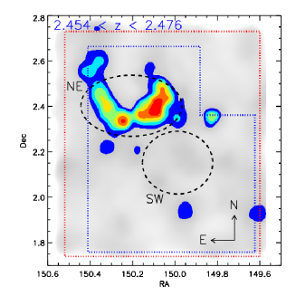
Figure 1: RA- Dec overdensity maps, in three redshift slices as indicated in the labels. The background grey-scale indicates the overdensity ${\rm log}(1+\delta_{\rm gal})$ value (darker grey is for higher values). Regions with ${\rm log}(1+\delta_{\rm gal})$ above 2, 3, 4, 5, 6, and 7 $\sigma_{\rm\delta}$ above the mean are indicated with blue, cyan, green, yellow, orange, and red colours. respectively. The red dotted line encloses the region retained for the analysis, and the blue dotted line is the region covered by the VUDS survey. The two black dashed ellipses (repeated in all panels for reference) show the rough positions of the two main components of the proto-supercluster identified in this work, dubbed “NE” (rightmost panel) and “SW” (leftmost panel). The field dimensions in RA and Dec correspond roughly to $\sim 120\times 130$ cMpc in the redshift range spanned by the three redshift slices.

The method to compute the density field and identify the density peaks is the same as described in Lemaux et al. (2018); we describe it here briefly. The method is based on the Voronoi Tessellation, which has already been successfully used at different redshifts to characterise the local environment around galaxies and identify the highest density peaks, including the search for groups and clusters (see e.g. Marinoni et al. 2002; Cooper et al. 2005; Cucciati et al. 2010; Gerke et al. 2012; Scoville et al. 2013; Darvish et al. 2015; Smolčić et al. 2017). Its main advantage is that the local density is measured both on an adaptive scale and with an adaptive filter shape, allowing us to follow the natural distribution of tracers.

In our case, we worked in two dimensions in overlapping redshift slices. We used as tracers the spectroscopic sample complemented by a photometric sample which provides us with the photometric redshifts of all the galaxies for which we did not have any $z_{s}$ information.

For each redshift slice, we generated a set of Monte Carlo (MC) realisations. Galaxies (with $z_{s}$ or $z_{p}$) to be used in each realisation were selected observing the following steps, in this order:

• irrespectively of their redshift, galaxies with a $z_{s}$ were retained in a percentage of realisations equal to the probability associated to the reliability flag; namely, in each realisation, before the selection in redshift, for each galaxy we drew a number from a uniform distribution from 0 to 100 and retained that galaxy only if the drawn number was equal to or less than the galaxy redshift reliability;

• galaxies with only $z_{p}$ were first selected to complement the retained spectroscopic sample (i.e. the photometric sample comprises all the galaxies without a $z_{s}$ or for which we threw away their $z_{s}$ for a given iteration), then they were assigned a new photometric redshift $z_{\rm p,new}$ randomly drawn from an asymmetrical Gaussian distribution centred on their nominal $z_{p}$ value and with negative and positive sigmas equal to the lower and upper uncertainties in the $z_{p}$ measurement, respectively; with this approach we do not try to correct for catastrophic redshift errors, but only for the shape of the PDF of each $z_{p}$;

• among the samples selected at steps 1 and 2, we retained all the galaxies with $z_{s}$ (from step 1) or $z_{\rm p,new}$ (from step 2) falling in the considered redshift slice.

We performed a 2D Voronoi tessellation for each $i^{th}$ MC realisation, and assigned to each Voronoi polygon a surface density $\Sigma_{VMC,i}$ equal to the inverse of the area (expressed in Mpc²) of the given polygon. Finally, we created a regular grid of $75\times 75$ pkpc cells, and assigned to each grid point the $\Sigma_{VMC,i}$ of the polygon enclosing the central point of the cell. For each redshift slice, the final density field $\Sigma_{VMC}$ is computed on the same grid, as the median of the density fields among the realisations, cell by cell. As a final step, from the median density map we computed the local over-density at each grid point as $\delta_{\rm gal}=\Sigma_{VMC}/\tilde{\Sigma}_{VMC}-1$, where $\tilde{\Sigma}_{VMC}$ is the mean $\Sigma_{VMC}$ for all grid points. In our analysis we are more interested in $\delta_{\rm gal}$ than in $\Sigma_{VMC}$ because we want to identify the regions that are overdense with respect to the mean density at each redshift, a density which can change not only for astrophysical reasons but also due to characteristics of the imaging/spectroscopic survey. Moreover, as we see in the following sections, the computation of $\delta_{\rm gal}$ is useful to estimate the total mass of our proto-cluster candidates and their possible evolution.

Proto-cluster candidates were identified by searching for extended regions of contiguous grid cells with a $\delta_{\rm gal}$ value above a given threshold. The initial systematic search for proto-clusters in the COSMOS field (which will be presented in Lemaux et al., in prep.) was run with the following set of parameters: redshift slices of 7.5 pMpc shifting in steps of 3.75 pMpc (so as to have redshift slices overlapping by half of their depth); 25 Monte Carlo realisations per slice; and spectroscopic and photometric catalogues with $[3.6]\leq 25.3$ (IRAC Channel 1). With this ‘blind’ search we re-identified two proto-clusters at $z\sim 3$ serendipitously discovered at the beginning of VUDS observations (Lemaux et al. 2014; Cucciati et al. 2014), together with other outstanding proto-structures presented separately in companion papers (Lemaux et al. 2018, Lemaux et al. in prep.).

3 Discovery of a rich extended proto-supercluster

The preliminary overdensity maps showed two extended overdensities at $z\sim 2.46$, in a region of $0.4\times 0.25$ deg². Intriguingly, there were several other smaller overdensities very close in right ascension (RA), declination (Dec), and redshift. We therefore explored in more detail the COSMOS field by focusing our attention on the volume around these overdensities. This focused analysis revealed the presence of a rich extended structure, consisting of density peaks linked by slightly less dense regions.

3.1 The method

We re-ran the computation of the density field and the search for overdense regions with a fine-tuned parameter set (see below), in the range $2.35\lesssim z\lesssim 2.55$, which we studied by considering several overlapping redshift slices. Concerning the angular extension of our search, we computed the density field in the central $\sim 1\times 1$ deg² of the COSMOS field, but then used only the slightly smaller 0.91 deg² region at $149.6\leq RA\leq 150.52$ and $1.74\leq Dec\leq 2.73$ to perform any further analysis (computation of the mean density etc.). This choice was made to avoid the regions close to the field boundaries, where the Voronoi tessellation is affected by border effects. In this smaller area, considering a flux limit at $i=25$, about 24% of the objects with a redshift ($z_{s}$ or $z_{p}$) falling in the above-mentioned redshift range have a spectroscopic redshift. If we reduce the area to the region covered by VUDS observations, which is slightly smaller, this percentage increases to about 28%.

We also verified the robustness of our choices for what concerns the following issues:

Number of Monte Carlo realisations. With respect to Lemaux et al. (in prep.), we increased the number of Monte Carlo realisations from the initial 25 to 100 to obtain a more reliable median value (similarly to, e.g. Lemaux et al. 2018). We verified that our results did not significantly depend on the number of realisations $n_{\rm MC}$ as long as $n_{\rm MC}\geq 100$, and, therefore, all analyses presented in this paper are done on maps which used $n_{\rm MC}=100$. This high number of realisations allowed us to produce not only the median density field for each redshift slice, but also its associated error maps, as follows. For each grid cell, we considered the distribution of the 100 $\Sigma_{VMC}$ values, and took the $16^{th}$ and $84^{th}$ percentiles of this distribution as lower and upper limits for $\Sigma_{VMC}$. We produced density maps with these lower and upper limits, in the same way as for the median $\Sigma_{VMC}$, and then computed the corresponding overdensities that we call $\delta_{\rm gal,16}$ and $\delta_{\rm gal,84}$.

Spectroscopic sample. As in Lemaux et al. (2018), we assigned a probability to each spectroscopic galaxy to be used in a given realisation equal to the reliability of its $z_{s}$ measurement, as given by its quality flag. Namely, we used the quality flags X2 (X2.5 for zCOSMOS), X3, X4, and X9 with a reliability of 80%, 97.5%, 100% and 80% respectively (see Sect. 2; here we adopt the mean probability for the flags X2 and X3, for which Le Fèvre et al. 2015 give a range of probabilities). These values were computed for the VUDS survey, but we applied them also to the zCOSMOS spectroscopic galaxies in our sample, as discussed in Sect. 2. We verified that our results do not qualitatively change if we choose slightly different reliability percentages or if we used the entire spectroscopic sample (flag=X2/X2.5, X3, X4, X9) in all realisations instead of assigning a probability to each spectroscopic galaxy. The agreement between these results is due to the very high flag reliabilities, and to the dominance of objects with only $z_{p}$. With the cut in redshift at $2.35\leq z\leq 2.55$, the above-mentioned quality flag selection, and the magnitude limit at $i\leq 25$ (see below), we are left with 271 spectroscopic redshifts from VUDS and 309 from zCOSMOS, for a total of 580 spectroscopic redshifts used in our analysis. This provides us with a spectroscopic sampling rate of $\sim 24\%$, considering the above mentioned redshift range and magnitude cut. We remind the reader that we use only VUDS and zCOSMOS spectroscopic redshift, and do not include in our sample any other $z_{s}$ found in the literature.

Mean density. To compute the mean density $\tilde{\Sigma}_{VMC}$ we proceeded as follows. Given that $\Sigma_{VMC}$ has a log-normal distribution (Coles & Jones 1991), in each redshift slice we fitted the distribution of ${\rm log}(\Sigma_{VMC})$ of all pixels with a $3\sigma$-clipped Gaussian. The mean $\mu$ and standard deviation $\sigma$ of this Gaussian are related to the average density $\langle\Sigma_{VMC}\rangle$ by the equation $\langle\Sigma_{VMC}\rangle=10^{\mu}e^{2.652\sigma^{2}}$. We used this $\langle\Sigma_{VMC}\rangle$ as the average density $\tilde{\Sigma}_{VMC}$ to compute the density contrast $\delta_{gal}$. $\tilde{\Sigma}_{VMC}$ was computed in this way in each redshift slice.

Overdensity threshold. In each redshift slice, we fitted the distribution of ${\rm log}(1+\delta_{\rm gal})$ with a Gaussian, obtaining its $\mu$ and $\sigma$. We call these parameters $\mu_{\rm\delta}$ and $\sigma_{\rm\delta}$, for simplicity, although they refer to the Gaussian fit of the ${\rm log}(1+\delta_{\rm gal})$ distribution and not of the $\delta_{\rm gal}$ distribution. We then fitted $\mu_{\rm\delta}$ and $\sigma_{\rm\delta}$ as a function of redshift with a second-order polynomial, obtaining $\mu_{\rm\delta,fit}$ and $\sigma_{\rm\delta,fit}$ at each redshift. Our detection thresholds were then set as a certain number of $\sigma_{\rm\delta,fit}$ above the mean overdensity $\mu_{\rm\delta,fit}$, that is, as ${\rm log}(1+\delta_{\rm gal})\geq\mu_{\rm\delta,fit}(z_{\rm slice})+n_{\sigma}\sigma_{\rm\delta,fit}(z_{\rm slice})$, where $z_{\rm slice}$ is the central redshift of each slice, and $n_{\sigma}$ is chosen as described in Sects. 3.2 and 4. From now, when referring to setting a ‘$n_{\sigma}\sigma_{\rm\delta}$ threshold’ we mean that we consider the volume of space with ${\rm log}(1+\delta_{\rm gal})\geq\mu_{\rm\delta,fit}(z_{\rm slice})+n_{\sigma}\sigma_{\rm\delta,fit}(z_{\rm slice})$.

Slice depth and overlap. We used overlapping redshift slices with a full depth of 7.5 pMpc, which corresponds to $\delta z\sim 0.02$ at $z\sim 2.45$, running in steps of $\delta z\sim 0.002$. We also tried with thinner slices (5 pMpc), but we adopted a depth of 7.5 pMpc as a compromise between i) reducing the line of sight (l.o.s.) elongation of the density peaks (see Sect. 3.2) and ii) keeping a low noise in the density reconstruction. We define ‘noise’ as the difference between $\delta_{\rm gal}$ and its lower and upper uncertainties $\delta_{\rm gal,16}$ and $\delta_{\rm gal,84}$. The choice of small steps of $\delta z\sim 0.002$ is due to the fact that we do not want to miss the redshift where each structure is more prominent.

Tracers selection We fine-tuned our search method (including the $\delta_{\rm gal}$ thresholds etc…) for a sample of galaxies limited at $i=25$. We verified the robustness of our findings by using also a sample selected with $K_{S}\leq 24$ and one selected with ${\rm[3.6]}\leq 24$ (IRAC Channel 1). With these two latter cuts, in the redshift range $2.3\leq z\leq 2.6$ we have a number of galaxies with spectroscopic redshift corresponding to $\sim 87\%$ and $\sim 94\%$ of the number of spectroscopic galaxies with $i\leq 25$, respectively, but not necessarily the same galaxies, while roughly 65% and 85% more objects, respectively, with photometric redshifts entered in our maps than did with $i\leq 25$. Although the $K_{S}\leq 24$ and ${\rm[3.6]}\leq 24$ samples might be distributed in a different way in the considered volume because of the different clustering properties of different galaxy populations, with these samples we recovered the overdensity peaks in the same locations as with $i\leq 25$. Clearly, the $\delta_{\rm gal}$ distribution is slightly different, so the overdensity threshold that we used to define the overdensity peaks (see Sect. 4) encloses regions with slightly different shape with respect to those recovered with a sample flux-limited at $i\leq 25$. We defer a more precise analysis of the kind of galaxy populations which inhabit the different density peaks to future work.

Figure 1 shows three 2D overdensity ($\delta_{\rm gal}$) maps obtained as described above, in the redshift slices $2.422<z<2.444$, $2.438<z<2.460$, and $2.454<z<2.476$. We can distinguish two extended and very dense components at two different redshifts and different RA-Dec positions: one at $z\sim 2.43$, in the left-most panel, that we call the “South-West” (SW) component, and the other at $z\sim 2.46$, at higher RA and Dec, that we call here the “North-East” (NE) component (right-most panel). The NE and SW components seem to be connected by a region of relatively high density, shown in the middle panel of the figure. This sort of filament is particularly evident when we fix a threshold around $2\sigma_{\rm\delta}$, as shown in the figure. For this reason, we retained the $2\sigma_{\rm\delta}$ threshold as the threshold used to identify the volume of space occupied by this huge overdensity. As a reference, a $2\sigma_{\rm\delta}$ threshold corresponds to $\delta\sim 0.65$, while 3, 4, and 5$\sigma_{\rm\delta}$ thresholds correspond to $\delta\sim 1.1$, $\sim 1.7$, and $\sim 2.55$, respectively

To better understand the complex shape of the structure, we performed an analysis in three dimensions, as described in the following sub-section.

3.2 The 3D matter distribution

We built a 3D overdensity cube in the following way. First, we considered each redshift slice to be placed at $z_{\rm slice}$ along the line of sight, where $z_{\rm slice}$ is the central redshift of the slice. All the 2D maps were interpolated at the positions of the nodes in the 2D grid of the lowest redshift ($z=2.35$). This way we have a 3D data cube with RA-Dec pixel size corresponding to $\sim 75\times 75$ pkpc at $z=2.38$, and a l.o.s. pixel size equal to $\delta z\sim 0.002$ (see Sect. 3.1). From now on we use ‘pixels’ and ‘grid cells’ with the same meaning, referring to the smallest components of our data cube. We smoothed our data cube in RA and Dec with a Gaussian filter with sigma equal to 5 pixels. Along the l.o.s., we used instead a boxcar filter with a depth of 3 pixels. The shape and dimension of the smoothing in RA-Dec was chosen as a compromise between the two aims of i) smoothing the shapes of the Voronoi polygons and ii) not washing away the highest density peaks. The smoothing along the l.o.s. was done to link each redshift slice with the previous and following slice. Different choices on the smoothing filters do not significantly affect the 2D maps in terms of the shapes of the over-dense regions, and have only a minor effect on the values of $\delta_{\rm gal}$, even if the highest-density peaks risk to be washed away in case of excessive smoothing. We produced data cubes for the lower and upper limits of $\delta_{\rm gal}$ ($\delta_{\rm gal,16}$ and $\delta_{\rm gal,84}$) in the same way. These two latter cubes are used for the treatment of uncertainties in our following analysis.

Figure 1 shows that around the main components of the proto-supercluster there are less extended density peaks. Since we wanted to focus our attention on the proto-supercluster, we excluded from our analysis all the density peaks not directly connected to the main structure. To do this, we proceeded as follows: we started from the pixels of the 3D grid which are enclosed in the $2\sigma_{\rm\delta}$ contour of the “NE” region in the redshift slice $2.454<z<2.476$ (right panel of Fig. 1). Starting from this pixel set, we iteratively searched in the 3D cube for all the pixels, contiguous to the previous pixels set, with a ${\rm log}(1+\delta_{\rm gal})$ higher than $2\sigma_{\rm\delta}$ above the mean, and we added those pixels to our pixel set. We stopped the search when there were no more contiguous pixels satisfying the threshold on ${\rm log}(1+\delta_{\rm gal})$. In this way we define a single volume of space enclosed in a $2\sigma_{\rm\delta}$ surface, and we define our proto-supercluster as the volume of space comprised within this surface. The final 3D overdensity map of the proto-supercluster is shown in Fig. 2, with the three axes in comoving megaparsecs.

The 3D shape of the proto-supercluster is very irregular. The NE and SW components are clearly at different average redshifts, and have very different 3D shapes. Figure 2 also shows that both components contain some density peaks (visible as the reddest regions within the $2\sigma_{\rm\delta}$ surface) with a very high average $\delta_{\rm gal}$. We discuss the properties of these peaks in detail in Sect. 4.

The volume occupied by the proto-supercluster shown in Fig. 2 is about $9.5\times 10^{4}$ cMpc³ (obtained by adding up the volume of all the contiguous pixels bounded by the 2$\sigma_{\rm\delta}$ surface), and the average overdensity is $\langle\delta_{\rm gal}\rangle\sim 1.24$. We can give a rough estimate of the total mass $M_{\rm tot}$ of the proto-supercluster by using the formula (see Steidel et al. 1998):

$$M_{\rm tot}=\rho_{\rm m}V(1+\delta_{\rm m}),$$ (1)

where $\rho_{m}$ is the comoving matter density, $V$ the volume that encloses the proto-cluster and $\delta_{\rm m}$ the matter overdensity in our proto-cluster. We computed $\delta_{\rm m}$ by using the relation $\delta_{\rm m}=\langle\delta_{\rm gal}\rangle/b$, where $b$ is the bias factor. Assuming $b=2.55$, as derived in Durkalec et al. (2015) at $z\sim 2.5$ with roughly the same VUDS galaxy sample we use here, we obtain $M_{\rm tot}\sim 4.8\times 10^{15}{\rm M}_{\odot}$. There are at least two possible sources of uncertainty in this computation. The first is the chosen $\sigma_{\rm\delta}$ threshold. If we changed our threshold by $\pm 0.2\sigma_{\rm\delta}$ around our adopted value of $2\sigma_{\rm\delta}$, $\langle\delta_{\rm gal}\rangle$ would vary by $\sim\pm 10\%$ and the volume would vary by $\sim\pm 17\%$, for a variation of the estimated mass of $\sim\pm 15\%$ (a higher threshold means a higher $\langle\delta_{\rm gal}\rangle$ and a smaller volume, with a net effect of a smaller mass; the opposite holds when we use a lower threshold). Another source of uncertainty is related to the uncertainty in the measurement of $\delta_{\rm gal}$ in the 2D maps. If we had used the 3D cube based on $\delta_{\rm gal,16}$(/$\delta_{\rm gal,84}$), we would have obtained $\langle\delta_{\rm gal}\rangle\sim 1.23(/1.26)$ and a volume of 1.06(/0.75)$\times 10^{5}$ cMpc³, for an overall total mass $\sim 10$% larger (/ $\sim 20$% smaller). If we sum quadratically the two uncertainties, the very liberal global statistical error on the mass measurement is of about $+18\%/-25\%$. Irrespectively of the errors, it is clear that this structure has assembled an immense mass ($>2\times 10^{15}{\rm M}_{\odot}$) at very early times. This structure is referred to hereafter as the ”Hyperion proto-supercluster” or simply ”Hyperion” (officially PSC J1001$+$0218) due to its immense size and mass and because one of its subcomponents (peak [3], see Sect. 4.2.3) is broadly coincident with the Colossus proto-cluster discovered by Lee et al. (2016).

We remark that the volume computed in our data cube is most probably an overestimate, at the very least because it is artificially elongated along the l.o.s. This elongation is mainly due to 1) the photometric redshift error ($\Delta z\sim 0.1$ for $\sigma_{zp}=0.03(1+z)$ at $z=2.45$), 2) the depth of the redshift slices ($\Delta z\sim 0.02$) used to produce the density field, and 3) the velocity dispersion of the member galaxies, which might create the feature known as the Fingers of God ($\Delta z\sim 0.006$ for a velocity dispersion of $500\,{\rm km\,s}^{-1}$). Although the velocity dispersion should be important only for virialised sub-structures, these three factors should all work to surreptitiously increase the dimension of the structure along the l.o.s. and at the same time decrease the local overdensity $\delta_{\rm gal}$. In this transformation there is no mass loss (or, equivalently, the total galaxy counts remain the same, with galaxies simply spread on a larger volume). Therefore, the total mass of our structure, computed with Eq. 1, would not change if we used the real (smaller) volume and the real (higher) density instead of the elongated volume and its associated lower overdensity.

We also ran a simple simulation to verify the effects of the depth of the redshift slices on the elongation. We built a simple mock galaxy catalogue at $z=2.5$ following a method similar to that described in Tomczak et al. (2017), a method which is based on injecting a mock galaxy cluster and galaxy groups onto a sample of mock galaxies that are intended to mimic the coeval field. As in Tomczak et al. (2017), the three dimensional positions of mock field galaxies are randomly distributed over the simulated transverse spatial and redshift ranges, with the number of mock field galaxies set to the number of photometric objects within an identical volume in COSMOS at $z\sim 2.5$ that is devoid of known proto-structures. Galaxy brightnesses were assigned by sampling the $K-$band luminosity function of Cirasuolo et al. (2010), with cluster and group galaxies perturbed to slightly brighter luminosities (0.5 and 0.25 mag, respectively). Member galaxies of the mock cluster and groups were assigned spatial locations based on Gaussian sampling with $\sigma$ equal to 0.5 and 0.33 h${}_{70}^{-1}$ pMpc, respectively, and were scattered along the l.o.s. by imposing Gaussian velocity dispersions of 1000 and 500 km s^-1, respectively. We then applied a magnitude cut to the mock catalogue similar to that used in our actual reconstructions, applied a spectroscopic sampling rate of 20%, and, for the remainder of the mock galaxies, assigned photometric redshifts with precision and accuracy identical to those in our photometric catalogue at the redshift of interest. We then ran the exact same density field reconstruction and method to identify peaks as was run on our real data, each time varying the depth of the redshift slices used. Following this exercise, we observed a smaller elongation for decreasing slice depth, with a $\sim 40\%$ smaller elongation observed when dropping the slice size from 7.5 to 2.5 pMpc. This result confirmed that we need to correct for the elongation if we want to give a better estimate of the volume and/or the density of the structures in our 3D cube. We will apply a correction for the elongation to the highest density peaks found in the Hyperion proto-supercluster, as discussed in Sect. 4.

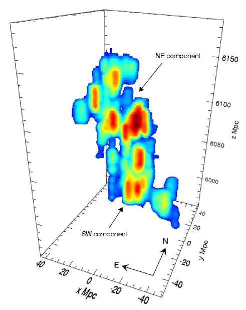
Figure 2: 3D overdensity map of the Hyperion proto-supercluster, in comoving megaparsecs. Colours scale with $\rm log(\sigma_{\rm\delta})$, exactly as in Fig. 1, from blue ($2\sigma_{\rm\delta}$) to the darkest red ($\sim 8.3\sigma_{\rm\delta}$, the highest measured value in our 3D cube). The $x-$, $y-$ and $z-$axes span the ranges $149.6\leq RA\leq 150.52$, $1.74\leq Dec\leq 2.73$ and $2.35\leq z\leq 2.55$. The NE and SW components are indicated. We highlight the fact that this figure shows only the proto-supercluster, and omits other less extended and less dense density peaks which fall in the plotted volume (see discussion in Sect. 3.2.)

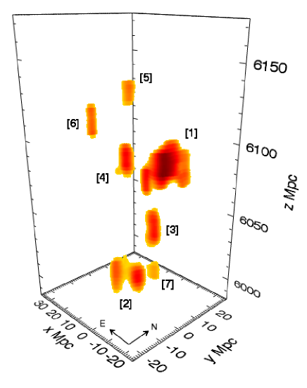
Figure 3: Zoom-in of Fig. 2. The angle of view is slightly rotated with respect to Fig. 2 so as to distinguish all the peaks. The colour scale is the same as in Fig. 2, but here only the highest density peaks are shown, that is, the 3D volumes where ${\rm log}(1+\delta_{\rm gal})$ is above the $5\sigma_{\rm\delta}$ threshold discussed in Sect. 4. Peaks are numbered as in Fig. 4 and Table 1.

4 The highest density peaks

We identified the highest density peaks in the 3D cube by considering only the regions of space with ${\rm log}(1+\delta_{\rm gal})$ above $5\sigma_{\rm\delta}$ from the mean density. In our work, this threshold corresponds to $\delta_{\rm gal}\sim 2.6$, which corresponds to $\delta_{m}\sim 1$ when using the bias factor $b=2.55$ found by Durkalec et al. (2015). We also verified, a posteriori, that with this choice we select density peaks which are about to begin or have just begun to collapse, after the initial phase of expansion (see Sect. 5). This is very important if we want to consider these peaks as proto-clusters.

With the overdensity threshold defined above, we identified seven separated high-density sub-structures. We show their 3D position and shape in Fig. 3. We computed the barycenter of each peak by weighting the $(x,y,z)$ position of each pixel belonging to the peak by its $\delta_{\rm gal}$. For each peak, we computed its volume, its $\langle\delta_{\rm gal}\rangle$, and derived its $M_{\rm tot}$ using Eq. 1 (the bias factor is always $b=2.55$, found by Durkalec et al. 2015 and discussed in Sect. 3.2). Table 1 lists barycenter, $\langle\delta_{\rm gal}\rangle$, volume, and $M_{\rm tot}$ of the seven peaks, numbered in order of decreasing $M_{\rm tot}$. We applied the same peak-finding procedure on the data cubes with $\delta_{\rm gal,16}$ and $\delta_{\rm gal,84}$, and computed the total masses of their peaks in the same way. We used these values as lower and upper uncertainties for the $M_{\rm tot}$ values quoted in the table.

From Table 1 we see that the overall range of masses spans a factor of $\sim 30$, from $\sim 0.09$ to $\sim 2.6$ times $10^{14}$M_⊙. The total mass enclosed within the peaks ($\sim 5.0\times 10^{14}$M_⊙) is about 10% of the total mass in the Hyperion proto-supercluster, while the volume enclosing all the peaks is a lower fraction of the volume of the entire proto-supercluster ($\sim 6.5\%$), as expected given the higher average overdensity within the peaks. The most massive peak (peak [1]) is included in the NE structure, together with peak [4] which has one fifth the total mass of peak [1]. Peak [2], which corresponds to the SW structure, has a $M_{\rm tot}$ comparable to peak [4], and it is located at lower redshift. Peak [3], with a $M_{\rm tot}$ similar to peaks [2] and [4], is placed in the sort of filament shown in the middle panel of Fig. 1. At smaller $M_{\rm tot}$ there is peak [5], with the highest redshift ($z=2.507$), and peak [6], at slightly lower redshift. They both have $M_{\rm tot}\sim 0.2\times 10^{14}$M_⊙. Finally, peak [7] is the least massive, and is very close in RA-Dec to peak [2], and at approximately the same redshift. In Appendix A.1 we show that the computation of $M_{\rm tot}$ is relatively stable if we slightly change the overdensity threshold used to define the peaks, with the exception of the least massive peak (peak [7]).

Figure 3 shows that the peaks have very different shapes, from irregular to more compact. We verified that their shape and position are not possibly driven by spectral sampling issues, by checking that the peaks persist through the $2^{\prime}$ gaps between the VIMOS quadrants from VUDS. This also implies that we are not missing high-density peaks that might fall in the gaps. We remind the reader that the zCOSMOS-Deep spectroscopic sample, which we use together with the VUDS sample, has a more uniform distribution in RA-Dec, and does not present gaps.

Concerning the shape of the peaks, we tried to take into account the artificial elongation along the l.o.s.. As mentioned at the end of Sect. 3.2, this elongation is probably due to the combined effect of the velocity dispersion of the member galaxies, the depth of the redshift slices, and the photometric redshift error (although we refer the reader to e.g. Lovell et al. 2018 for an analysis of the shapes of proto-clusters in simulations). We used a simple approach to give an approximate statistical estimate of this elongation, starting from the assumption that on average our peaks should have roughly the same dimension in the $x$, $y,$ and $z$ dimensions, and any measured systematic deviation from this assumption is artificial. In each of the three dimensions we measured a sort of effective radius $R_{e}$ defined as $R_{e,x}=\sqrt{\sum_{i}w_{i}(x_{i}-x_{peak})^{2}/\sum_{i}(w_{i})}$ (and similarly for $R_{e,y}$ and $R_{e,z}$), where the sum is over all the pixels belonging to the given peak, the weight $w_{i}$ is the value of $\delta_{\rm gal}$, $x_{i}$ the position in cMpc along the $x-$axis and $x_{peak}$ is the barycenter of the peak along the $x-$axis, as listed in Table 1. We defined the elongation $E_{\rm z/xy}$ for each peak as the ratio between $R_{e,z}$ and $R_{e,xy}$, where $R_{e,xy}$ is the mean between $R_{e,x}$ and $R_{e,y}$. The effective radii and the elongations are reported in Table 2. If the measured volume $V_{\rm meas}$ of our peaks is affected by this artificial elongation, the real corrected volume is $V_{\rm corr}=V_{\rm meas}/E_{\rm z/xy}$. Moreover, given that the elongation has the opposite and compensating effects of increasing the volume and decreasing $\delta_{\rm gal}$, as discussed at the end of Sect. 3.2, $M_{\rm tot}$ remains the same. For this reason, inverting Eq. 1 it is possible to derive the corrected (higher) average overdensity $\langle\delta_{\rm gal,corr}\rangle$ for each peak, by using $V_{\rm corr}$ and the mass in Table 1. $V_{\rm corr}$ and $\langle\delta_{\rm gal,corr}\rangle$ are listed in Table 2. We note that by definition $R_{e}$ is smaller than the total radial extent of an overdensity peak, because it is computed by weighting for the local $\delta_{\rm gal}$, which is higher for regions closer to the centre of the peak. For this reason, the $V_{\rm corr}$ values are much larger than the volumes that one would naively obtain by using $R_{e,xy}$ as intrinsic total radius of our peaks. We use $\langle\delta_{\rm gal,corr}\rangle$ in Sect. 5 to discuss the evolution of the peaks. We refer the reader to A.3 for a discussion on the robustness of the computation of $E_{\rm z/xy}$ and its empirical dependence on $R_{e,xy}$.

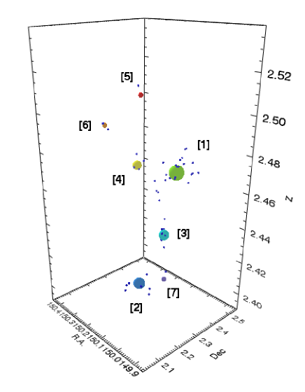
Figure 4: Same volume of space as Fig. 3, but in RA-Dec-$z$ coordinates. Each sphere represents one of the overdensity peaks, and is placed at its barycenter (see Table 1). The colour of the spheres scales with redshift (blue = low $z$, dark red = high $z$), and the dimension scales with the logarithm of $M_{\rm tot}$ quoted in Table 1. Small blue dots are the spectroscopic galaxies which are members of each overdensity peak, as described in Sect.4.

We also assigned member galaxies to each peak. We defined a spectroscopic galaxy to be a member of a given density peak if the given galaxy falls in one of the $\geq 5\sigma_{\delta}$ pixels that comprise the peak. The 3D distribution of the spectroscopic members is shown in Fig. 4, where each peak is schematically represented by a sphere placed in a $(x,y,z)$ position corresponding to its barycenter. It is evident that the 3D distribution of the member galaxies mirrors the shape of the peaks (see Fig. 3). The number of spectroscopic members $n_{\rm zs}$ is quoted in Table 1. The most extended and massive peak, peak [1], has 24 spectroscopic members. All the other peaks have a much smaller number of members (from 7 down to even only one member). We remind the reader that these numbers depend on the chosen overdensity threshold used to define the peaks, because the threshold defines the volume occupied by the peaks. Moreover, here we are counting only spectroscopic galaxies with good quality flags (see Sect. 2) from VUDS and zCOSMOS, excluding other spectroscopic galaxies identified in the literature (but see Sect. 4.1 for the inclusion of other samples to compute the velocity dispersion).

4.1 Velocity dispersion and virial mass

We computed the l.o.s. velocity dispersion $\sigma_{\rm v}$ of the galaxies belonging to each peak. For this computation we used a more relaxed definition of membership with respect to the one described above, so as to include also the galaxies residing in the tails of the velocity distribution of each peak. Basically, we used all the available good-quality spectroscopic galaxies within $\pm 2500\,{\rm km\,s}^{-1}$ from $z_{\rm peak}$ comprised in the RA-Dec region corresponding to the largest extension of the given peak on the plane of the sky. Moreover, we did not impose any cut in $i-$band magnitude, because, in principle, all galaxies can serve as reliable tracers of the underlying velocity field. We also included in this computation the spectroscopic galaxies with lower quality flag (flag = X1 for VUDS, all flags with X1.5$\leq$flag$<$2.5 for zCOSMOS), but only if they could be defined members of the given peak, with membership defined as at the end of the previous section. This less restrictive choice allows us to use more galaxies per peak than the pure spectroscopic members, although we still have only $\leq 4$ galaxies for three of the peaks. We quote these larger numbers of members in Table 3.

With these galaxies, we computed $\sigma_{\rm v}$ for each peak by applying the biweight method (for peak [1]) or the gapper method (for all the other peaks), and report the results of these computations in Table 3. The choice of these methods followed the discussion in Beers et al. (1990), where they show that for the computation of the scale of a distribution the gapper method is more robust for a sample of $\lesssim 20$ objects (all our peaks but peak [1]), while it is better to use the biweight method for $\gtrsim 20$ objects (our peak [1]). We computed the error on $\sigma_{\rm v}$ with the bootstrap method, which was taken as the reference method in Beers et al. (1990). In the case of peak [7], with only three spectroscopic galaxies available to compute $\sigma_{\rm v}$, we had to use the jack-knife method to evaluate the uncertainty on $\sigma_{\rm v}$; see also Sect. A.2 for more details on $\sigma_{\rm v}$ of peak [7].

We found a range of $\sigma_{\rm v}$ between $320\,{\rm km\,s}^{-1}$ and $731\,{\rm km\,s}^{-1}$. The most massive peak, peak [1], has the largest velocity dispersion, but for the other peaks the ranking in $M_{\rm tot}$ is not the same as in $\sigma_{\rm v}$. The uncertainty on $\sigma_{\rm v}$ is mainly driven by the number of galaxies used to compute $\sigma_{\rm v}$ itself, and it ranges from $\sim 12$% for peak [1] to $\sim 65$% for peak [7], for which we used only three galaxies to compute $\sigma_{\rm v}$. As we see below, other identifications in the literature of high-density peaks at the same redshift cover broadly the same $\sigma_{\rm v}$ range.

As we already mentioned, there are some works in the literature that identified/followed up some overdensity peaks in the COSMOS field at $z\sim 2.45$, such as for example Casey et al. (2015), Diener et al. (2015), Chiang et al. (2015), and Wang et al. (2016). Moreover, the COSMOS field has also been surveyed with spectroscopy by other campaigns, such as for example the COSMOS AGN spectroscopic survey (Trump et al. 2009), the MOSDEF survey (Kriek et al. 2015), and the DEIMOS 10K spectroscopic survey (Hasinger et al. 2018). We collected the spectroscopic redshifts of these other samples (including in this search also much smaller samples, like e.g. the one by Perna et al. 2015), removed the possible duplicates with our sample and between samples, and assigned these new objects to our peaks, by applying the same membership criterion as applied to our VUDS$+$zCOSMOS sample. We re-computed the velocity dispersion using our previous sample plus the new members found in the literature. We note that many objects in the COSMOS field have been observed spectroscopically multiple times, and in most of the cases the new redshifts were concordant with previous observations. This is a further proof of the robustness of the $z_{s}$ we use here.

In the literature we only find new members for the peaks [1], [3], [4], and [5]. For each of these peaks, Table 3 reports the number $n_{\rm lit}$ of spectroscopic redshifts added to our original sample, together with the new estimates of $\sigma_{\rm v}$ and $M_{\rm vir}$. The new $\sigma_{\rm v}$ is always in very good agreement (below $1\sigma$) with our previous computation, but it has a smaller uncertainty. We will see that this translates into new $M_{\rm vir}$ values which are in very good agreement with those based on the original $\sigma_{\rm v}$.

As a by-product of the use of the spectroscopic member galaxies, we also computed a second estimate of the redshift of each peak (after the barycenter, see above). Beers et al. (1990) show that the biweight method is the most robust to compute the central location of a distribution of objects (in our case, the average redshift) also in the case of relatively few objects ($5-50$). This central redshift, $z_{\rm BI}$, is reported in Table 3, and is in excellent agreement with $z_{\rm peak}$, that is, the barycenter along the l.o.s. quoted in Table 1.

The use of the gapper and/or biweight methods is to be favoured when estimating the scale of a distribution also because they apply when the distribution is not necessarily a Gaussian, and certainly the shape of the galaxy velocity distribution in a proto-cluster may not follow a Gaussian distribution. In addition, it is questionable to assume that proto-clusters are virialised systems. Nevertheless, a crude way to estimate the mass of the peaks is to assume the validity of the virial theorem. In this way we can estimate the virial mass $M_{\rm vir}$ by using the measured velocity dispersion and some known scaling relations. We follow the same procedure as Lemaux et al. (2012), where $M_{\rm vir}$ is defined as:

$$M_{\rm vir}=\frac{3\sqrt{3}\sigma_{\rm v}^{3}}{\alpha\leavevmode\nobreak\ 10\leavevmode\nobreak\ G\leavevmode\nobreak\ H(z)}.$$ (2)

In Eq. 2, $\sigma_{\rm v}$ is the line of sight velocity dispersion, $G$ is the gravitational constant, and $H(z)$ is the Hubble parameter at a given redshift. Equation 2 is derived from i) the definition of the virial mass,

$$M_{\rm vir}=\frac{3}{G}\sigma_{\rm v}^{2}\leavevmode\nobreak\ R_{\rm v},$$ (3)

where $R_{\rm v}$ is the virial radius; ii) the relation between $R_{\rm 200}$ and $R_{\rm v}$,

$$R_{\rm 200}=\alpha\leavevmode\nobreak\ R_{\rm v},$$ (4)

where $R_{\rm 200}$ is the radius within which the density is 200 times the critical density, and iii) the relation between $R_{\rm 200}$ and $\sigma_{\rm v}$,

$$R_{\rm 200}=\frac{\sqrt{3}\leavevmode\nobreak\ \sigma_{\rm v}}{10\leavevmode\nobreak\ H(z)}.$$ (5)

Equations 3 and 5 are from Carlberg et al. (1997). Differently from Lemaux et al. (2012), we use $\alpha\simeq 0.93$, which is derived comparing the radii where a NFW profile with concentration parameter $c=3$ encloses a density 200 times ($R_{\rm 200}$) and 173 times ($R_{\rm v}$) the critical density at $z\simeq 2.45$. Here we consider a structure to be virialised when its average overdensity is $\Delta_{\rm v}\simeq 173$, which corresponds, in a $\Lambda$CDM Universe at $z\simeq 2.45$, to the more commonly used value $\Delta_{\rm v}\simeq 178$, constant at all redshifts in an Einstein-de Sitter Universe (see the discussion in Sect. 5.1).

The virial masses of our density peaks, computed with Eq. 2, are listed in Table 3, together with the virial masses obtained from the $\sigma_{\rm v}$ computed by using also other spectroscopic galaxies in the literature. Figure 5 shows how our $M_{\rm vir}$ compared with the total masses $M_{\rm tot}$ obtained with Eq. 1. For four of the seven peaks, the two mass estimates basically lie on the 1:1 relation. In the three other cases, the virial mass is higher than the mass estimated with the overdensity value: namely, for peaks [4] and [5] the agreement is at $<2\sigma$, while for peak [7] the agreement is at less than $1\sigma$ given the very large uncertainty on $M_{\rm vir}$.

The overall agreement between the two sets of masses is surprisingly good, considering that $M_{\rm vir}$ is computed under the strong (and probably incorrect) assumption that the peaks are virialised, and that $M_{\rm tot}$ is computed above a reasonable but still arbitrary density threshold. Indeed, although the adopted density threshold corresponds to selecting peaks which are about to begin or have just begun to collapse (see Sect. 4), the evolution of a density fluctuation from the beginning of collapse to virialisation can take a few gigayears (see Sect. 5). Moreover, the galaxies used to compute $\sigma_{v}$ and hence $M_{\rm vir}$ are drawn from slightly larger volumes than the volumes used to compute $M_{\rm tot}$, because we included galaxies in the tails of the velocity distribution along the l.o.s., outside the peaks’ volumes. We also find that $M_{\rm tot}$ continuously varies by changing the overdensity threshold to define the peaks (see Appendix A.1), while the computation of the velocity dispersion in our peaks is very stable if we change this same threshold (see Appendix A.2). As a consequence, we do not expect the estimated $M_{\rm vir}$ to change either. In addition to these caveats, peaks [1], [2] and [3] show an irregular 3D shape (see Appendix B), and they might be multi-component structures. In these cases, the limited physical meaning of $M_{\rm vir}$ is evident.

We also note that peak [5] has already been identified in the literature as a virialised structure (see Wang et al. 2016 and our discussion in Sect. 4.2.5), meaning that its $M_{\rm vir}$ is possibly the most robust among the peaks, but in our reconstruction it is the most distant from the 1:1 relation between $M_{\rm vir}$ and $M_{\rm tot}$. This might suggest that our $M_{\rm tot}$ is underestimated, at least for this peak.

We also remark that there is not a unique scaling relation between $\sigma_{\rm v}$ and $M_{\rm vir}$. For instance, Munari et al. (2013) study the relation between the masses of groups and clusters and their 1D velocity dispersion $\sigma_{\rm 1D}$. Clusters are extracted from $\Lambda$CDM cosmological N-body and hydrodynamic simulations, and the authors recover the velocity dispersion by using three different tracers, that is, dark-matter particles, sub-halos, and member galaxies. They find a relation in the form:

$$\sigma_{\rm 1D}=A_{1D}\left[\frac{h(z)\leavevmode\nobreak\ M_{\rm 200}}{10^{15}M_{\odot}}\right]^{\alpha},$$ (6)

where $A_{1D}\simeq 1180\,{\rm km\,s}^{-1}$ and $\alpha\simeq 0.38$, as from their Fig. 3 for $z=2$ (the highest redshift they consider) and by using galaxies as tracers for $\sigma_{\rm 1D}$. Evrard et al. (2008) find a relation based on the same principle as Eq. 6, but they use DM particles to trace $\sigma_{\rm 1D}$. On the observational side, Sereno & Ettori (2015) find a relation in perfect agreement with Munari et al. (2013) by using observed data, with cluster masses derived via weak lensing. We also used Eq. 6 to compute $M_{\rm vir}$. We found that the $M_{\rm vir}$ computed via Eq. 6 are systematically smaller (by 20-40%) than the previous ones computed with Eq. 2. This change would not appreciably affect the high degree of concordance between $M_{\rm vir}$ and $M_{\rm tot}$ for our peaks.

In summary, the comparison between $M_{\rm vir}$ and $M_{\rm tot}$ is meaningful only if we fully understand the evolutionary status of our overdensities and know their intrinsic shapes (and we remind the reader that in this work the shape of the peaks depends at the very least on the chosen threshold, and it is not supposed to be their intrinsic shape). On the other hand, it would be very interesting to understand whether it is possible to use this comparison to infer the level of virialisation of a density peak, provided that its shape is known. This might be studied with simulations, and we defer this analysis to a future work.

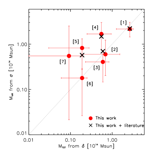
Figure 5: Virial mass $M_{\rm vir}$ of the seven identified peaks, as in Table 3, vs. the total mass $M_{\rm tot}$ as in Table 1. We show both the virial mass computed only with our spectroscopic sample (red dots, column 6 of Table 3) and how it would change if we add to our sample other spectroscopic sources found in the literature (black crosses, column 9 of Table 3). Only peaks [1], [3], [4], and [5] have this second estimate of $M_{\rm vir}$. The dotted line is the bisector, as a reference.

4.2 The many components of the proto-supercluster

The COSMOS field is one of the richest fields in terms of data availability and quality. It was noticed early on that it contains extended structures at several redshifts (see e.g. Scoville et al. 2007; Guzzo et al. 2007; Cassata et al. 2007; Kovač et al. 2010; de la Torre et al. 2010; Scoville et al. 2013; Iovino et al. 2016). Besides using galaxies as direct tracers, as in the above-mentioned works, the large-scale structure of the COSMOS field has been revealed with other methods like weak lensing analysis (e.g. Massey et al. 2007) and Ly$\alpha$-forest tomography (Lee et al. 2016, 2018). Systematic searches for galaxy groups and clusters have also been performed up to $z\sim 1$ (for instance Knobel et al. 2009 and Knobel et al. 2012), and in other works we find compilations of candidate proto-groups (Diener et al. 2013) and candidate proto-clusters (Chiang et al. 2014; Franck & McGaugh 2016; Lee et al. 2016) at $z\gtrsim 1.6$. In some cases, the search for (proto-)clusters was focused around a given class of objects, like radio galaxies (see e.g. Castignani et al. 2014).

In particular, it has been found that the volume of space in the redshift range $2.4\lesssim z\lesssim 2.5$ hosts a variety of high-density peaks, which have been identified by means of different techniques/galaxy samples, and in some cases as part of dedicated follow-ups of interesting density peaks found in the previous compilations. Some examples are the studies by Diener et al. (2015), Chiang et al. (2015), Casey et al. (2015), Lee et al. (2016), and Wang et al. (2016). In this paper, we generally refer to the findings in the literature as density peaks when referring to the ensemble of the previous works; we use the definition adopted in each single paper (e.g. ‘proto-groups’, ‘proto-cluster candidates’, etc.) when we mention a specific study.

We note that in the vast majority of these previous works there was no attempt to put the analysed density peaks in the broader context of a large-scale structure. The only exceptions are the works by Lee et al. (2016) and Lee et al. (2018), based on the Ly$\alpha$-forest tomography. Lee et al. (2016) explore an area of $\sim 14\times 16$ h^-1 cMpc, which is roughly one ninth of the area covered by Hyperion, while Lee et al. (2018) extended the tomographic map up to an area roughly corresponding to one third of the area spanned by Hyperion. Both these works do mention the complexity and the extension of the overdense region at $z\sim 2.45$, and the fact that it embeds three previously identified overdensity peaks (Diener et al. 2015; Casey et al. 2015; Wang et al. 2016). Nevertheless, they did not expand on the characteristics of this extended region, and were unable to identify the much larger extension of Hyperion, because of the smaller explored area.

In this section we describe the characteristics of our seven peaks, and compare our findings with the literature. The aim of this comparison is to show that some of the pieces of the Hyperion proto-supercluster have already been sparsely observed in the literature, and with our analysis we are able to add new pieces and put them all together into a comprehensive scenario of a very large structure in formation. We also try to give a detailed description of the characteristics (such as volume, mass, etc.) of the structures already found in the literature, with the aim to show that different selection methods are able to find the same very dense structures, but these methods in some cases are different enough to give disparate estimates of the peaks’ properties. For this comparison, we refer to Fig. 6 and Table 4, as detailed below. Moreover, in Appendix B we show more details on our four most massive peaks, which we dub “Theia”, “Eos”, “Helios”, and “Selene”. Among the previous findings, we discuss only those falling in the volume where our peaks are contained. We remind that we did not make use of the samples used in these previous works. The only exception is that the zCOSMOS-Deep sample, included in our data set, was also used by Diener et al. (2013).

4.2.1 Peak [1] - “Theia”

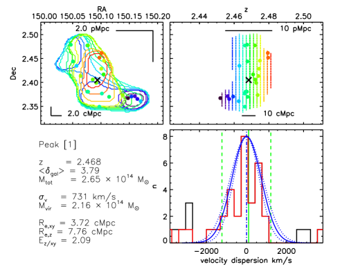
Figure 10: For peak [1], “Theia”, the top-left panel show the projection on the RA-Dec plane of the $5\sigma_{\rm\delta}$ contours which identify the peak in the 3D overdensity cube; the different colours indicate the different redshift slices (from blue to red, they go from the lowest to the highest redshift). Filled circles are the spectroscopic galaxies which are members of the peak (flag=X2/X2.5, X3, X4, X9), with the same colour code as the the contours. The black cross is the RA-Dec barycenter of the peak. In the top-right and bottom-left corners we show the scale in pMpc and cMpc, respectively, for both RA and Dec. Top-right. Projections on the $z$-Dec plane of the same contours shown in the top-left panel, with the same colour code. The filled circles and the black cross are as in the top-left panel. On the top and on the bottom of the panel we show the scale in pMpc and cMpc, respectively. Bottom-right. The black histogram represents the velocity distribution of the spectroscopic galaxies which fall in the same RA-Dec region as the proto-cluster. The red histogram includes only VUDS and zCOSMOS galaxies with reliable quality flag, and flags X1/X1.5 for galaxies within the peak volume (see Sect. 4.1 for details). The vertical solid green line indicates the barycenter along the l.o.s (the top x-axis is the same as the one in the top-right panel), and the two dashed vertical lines the maximum extent of the peak. The dotted-dashed blue vertical line is the $z_{\rm BI}$ of Table 3, around which we center the Gaussian (blue solid curve) with the same $\sigma_{v}$ as in Table 3. The two dotted blue curves are the uncertainties on the Gaussian due to the uncertainties on $\sigma_{v}$. In the bottom-left corner of the figure we summarise some of the peak properties, which are all already mentioned in the Tables or in the text.

Peak [1] is by far the most massive of the peaks we detected. Figure 3 shows that its shape is quite complex. The peak is composed of two substructures that indeed become two separated peaks if we increase the threshold for the peak detection from $5\sigma_{\delta}$ to $6.6\sigma_{\delta}$. In Fig. 10 of Appendix B we show two 2D projections of peak [1], which indicate the complexity of the 3D structure of this peak.

Figure 6 is the same as Fig. 3, but we also added the position of the overdensity peaks found in the literature. We verified that our peak [1] includes three of the proto-groups in the compilation by Diener et al. (2013), called D13a, D13b, and D13d in our figure. Proto-goups D13a and D13b are very close to each other ($\sim 3$ arcmin on the RA-Dec plane) and together they are part of the main component of our peak [1]. D13d corresponds to the secondary component of peak [1], which detaches from the main component when we increase the overdensity threshold to $6.6\sigma_{\delta}$. Another proto-group (D13e) found by Diener et al. (2013) falls just outside the westernmost and northernmost border of peak[1]. It is not unexpected that our peaks (see also peaks [3] and [4]) have a good match with the proto-groups found by Diener et al. (2013), given that their density peaks have been detected using the zCOSMOS-Deep sample, which is also included in our total sample. In our peak [1] we find 24 spectroscopic members (see Table 1), 14 of which come from the VUDS survey and 10 from the zCOSMOS-Deep sample.

The shape of peak[1] (a sort of ‘L’, or triangle) is mirrored by the shape of the proto-cluster found by Casey et al. (2015), as shown in their Fig. 2. In our Fig. 6 their proto-cluster is marked as Ca15, and we placed it roughly at the coordinates of the crossing of the two arms of the ‘L’ in their figure, where they found an X-ray detected source. In their figure, the S-N arm extends to the north and has a length of $\sim 14$ arcmin, and the E-W arm extends towards east and its length is about 10 arcmin. They also show that their proto-cluster encloses the three proto-groups D13a, D13b, and D13d.

Although we found a correspondence between the position/extension of our peak [1] and the position/extension of some overdensities in the literature, it is harder to compare the properties of peak [1] and such overdensities. This difficulty is given mainly by the different detection techniques. We attempted this comparison and show the results in Table 4. In this table, for each overdensity in the literature we show its redshift, $\delta_{\rm gal}$, velocity dispersion, and total mass, when available in the respective papers. We also computed its total volume, based on the information in its respective paper, and computed its $\delta_{\rm gal}$ and total mass (using Eq. 1) in that same volume in our 3D cube. In the case of a 1:1 match with our peak (like in the case of Ca15 and our peak [1]), we also reported the properties of our matched peak.

In the case of the proto-groups D13a, D13b, D13d and D13e, we found in the literature only their $\sigma_{\rm v}$, which we cannot compare directly with our peak [1] given that there is not a 1:1 match. The $\delta_{\rm gal}$ recovered in our 3D cube in the volumes corresponding to the four proto-groups are broadly consistent with the typical $\delta_{\rm gal}$ of our peaks, with the exception of D13e which in fact falls outside our peak [1]. These proto-groups have all relatively small volumes and masses compared to our peaks. At most, the largest one (D13a) is comparable in volume and mass with our smallest peaks ([5],[6], and [7]). The average difference in volume between our peaks and the proto-groups found in Diener et al. (2013) might be due to the fact that they identified groups with a Friend-of-Friend algorithm with a linking length of 500 pkpc, i.e. $\sim 1.7$ cMpc at $z=2.45$, which is smaller than the effective radius of our largest peaks (although their linking lengths and our effective radii do not have the same physical meaning).

The properties of Ca15 were computed in a volume almost three times as large as our peak [1]. Nevertheless, its $\delta_{\rm gal}$ is much higher, probably because of the different tracers (they use dusty star forming galaxies, ‘DSFGs’). Despite our lower density in the Ca15 volume, we find a higher total mass ($M_{\rm tot}=4.82\times 10^{14}M_{\odot}$ instead of their total mass of $>0.8\times 10^{14}M_{\odot}$). This is probably due to the different methods used to compute $M_{\rm tot}$: we use Eq. 1, while Casey et al. (2015) use abundance matching techniques to assign a halo mass to each galaxy, and then sum the estimated halo masses for each galaxy in the structure. Moreover, they state that their mass estimate is a lower limit.

4.2.2 Peak [2] - “Eos”

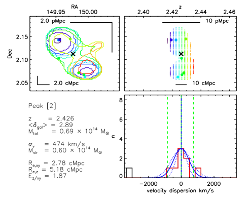
Figure 11: As in Fig.10, but for Peak [2], “Eos”.

As peak [1], this peak seems to be composed by two sub-structures, as shown in details in Fig. 11. The two substructures detach from each other when we increase the overdensity threshold to $5.3\sigma_{\delta}$. On the contrary, by decreasing the overdensity threshold to $4.5\sigma{\delta}$ we notice that this peak merges with the current peak [7].

We did not find any direct match of peak [2] with previous detections of proto-structures in the literature. We note that this part of the COSMOS field is only partially covered by the tomographic search performed by Lee et al. (2016) and Lee et al. (2018). This could be the reason why they do not find any prominent density peak there.

4.2.3 Peak [3] - “Helios”

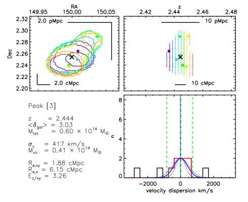
Figure 12: As in Fig.10, but for Peak [3], “Helios”.

The detailed shape of peak [3] is shown in Fig. 12. From our density field, it is hard to say whether its shape is due to the presence of two sub-structures. Even by increasing the overdensity threshold, the peak does not split into two sub-components.

Peak [3] is basically coincident with the group D13f from Diener et al. (2013), and its follow-up by Diener et al. (2015), which we call D15 in our Fig. 6. The barycenter of our peak [3] is closer to the position of D13f than to the position of D15, on both the RA-Dec plane ($<8^{\prime\prime}$ to D13f, $\sim 50^{\prime\prime}$ on the Dec axis to D15) and the redshift direction ($\Delta z\sim 0.004$ with D13f, and $\Delta z\sim 0.05$ with D15). This very good match is possibly due also to the fact that our sample includes the zCOSMOS-Deep data (see comment in Sect. 4.2.1). Indeed, out of the seven spectroscopic members that we identified in peak [3], five come from the zCOSMOS-Deep sample and two from VUDS. We note that the list of candidate proto-clusters by Franck & McGaugh (2016) includes a candidate that corresponds, as stated by the authors, to D13f. Interestingly, Diener et al. (2015) mention that D15 might be linked to the radio galaxy COSMOS-FRI 03 (Chiaberge et al. 2009), around which Castignani et al. (2014) found an overdensity of photometric redshifts. Although the overdensity of photometric redshifts surrounding the radio galaxy is formally at slightly lower redshift than D15 (see also Chiaberge et al. 2010), it is possibly identifiable with D15, given the photometric redshift uncertainty.

Table 4 shows that the velocity dispersion found by Diener et al. (2015) for D15 is very similar to the one we find for our peak [3], although the density that they recover is much larger ($\delta_{\rm gal}=10$ vs $\delta_{\rm gal}\sim 3.$). We note that D15 is defined over a volume which is almost twice as large as peak [3]. The velocity dispersion of F16 is instead almost double the one we recover for peak [3]. Their search volume is huge ($\sim 10000$ cMpc³) compared to the volume of peak [3]. Considering that they also find quite high $\delta_{\rm gal}$, they compute a total mass of $\sim 15\times 10^{14}$ M_⊙, which is approximately three times larger than the one we find in our data in their same volume ($4.89\times 10^{14}$ M_⊙), but about a factor of 30 larger than the mass of our peak [3].

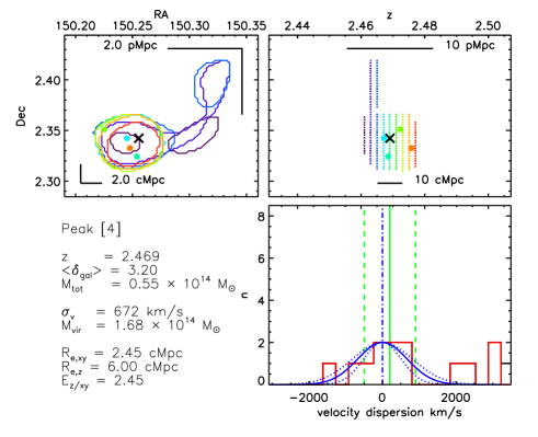
Figure 13: As in Fig.10, but for Peak [4], “Selene”.

Very close to peak [3] there are the three components of the extended proto-cluster dubbed ‘Colossus’ in Lee et al. (2016). Here we call the three sub-structures L16a, L16b and L16c, in order of decreasing redshift. This proto-cluster was detected by IGM tomography (see also Lee et al. 2018) performed by analysing the spectra of galaxies in the background of the proto-cluster. The three peaks form a sort of chain from $z\sim 2.435$ to $z\sim 2.45$, which extends over $\sim 2^{\prime}$ in RA and $\sim 6^{\prime}$ in Dec. We derived the positions of the first and third peaks from Fig. 12 of Lee et al. (2016), and assumed that the intermediate peak was roughly in between (see their Figs. 4 and 13). Neither L16a, L16b, or L16c coincide precisely with one of our peaks, but they fall roughly 3 arcmin eastwards of the barycenter of our peak [3]. The declination and redshift of the intermediate component correspond to those of our peak [3]. Given the extension of the three peaks in RA-Dec (they have a radius from $\sim 2$ to $\sim 4$ arcmin) and the extension of our peak [3] ($\sim 2$ arcmin radius), the ‘Colossus’ overlaps with, and it might be identified with, our peak [3].

Lee et al. (2016) compute the total mass of their overdensity, and find that it is $1.6\pm 0.9\times 10^{14}$ M_⊙. Computing the overall mass in the volumes of the three components L16a, L16b, and L16c in our data cube, we find a smaller mass ($0.83\times 10^{14}$ M_⊙), which is still consistent with the value found by Lee et al. (2016).

We additionally compared our results with those by Lee et al. (2016) by directly using the smoothed IGM overdensity, $\delta_{F}^{\rm sm}$, estimated from the latest tomographic map (Lee et al. 2018). We measured their average $\delta_{F}^{\rm sm}$ in the volume enclosing our peak [3] and found that this volume of space corresponds to an overdense region with respect to the mean intergalactic medium (IGM) density at these redshifts. Specifically, using the definition in Lee et al. (2016), for which negative values of $\delta_{F}^{\rm sm}$ signify overdense regions, we found that our peak has $\langle\delta_{F}^{\rm sm}\rangle\sim-2.4\sigma_{\rm sm}$, with $\sigma_{\rm sm}$ denoting the effective sigma of the $\delta_{F}^{\rm sm}$ distribution. We repeated the same analysis in the volumes enclosed by our other peaks (with the exception of peak [2], which lies almost entirely outside the tomographic map), and we found that their $\langle\delta_{F}^{\rm sm}\rangle$ fall in the range from $-1.9\sigma_{\rm sm}$ to $-1\sigma_{\rm sm}$ meaning that all of our peaks appear overdense with respect to the mean IGM density at these redshifts. This persistent overdensity measured across the six peaks that we are able to measure in the tomographic map strongly hint at a coherent overdensity also present in the IGM maps. Further, all peaks have measured $\langle\delta_{F}^{\rm sm}\rangle$ values consistent with the expected IGM absorption signal due to the presence of at least some fraction of simulated massive ($M_{\rm tot,z=0}>10^{14}M_{\odot}$) proto-clusters (see section 4 of Lee et al. 2016). We note, however, that none of our peaks have $\langle\delta_{F}^{\rm sm}\rangle<-3\sigma_{\rm sm}$, which is the threshold suggested by Lee et al. (2016) to safely identify proto-clusters (see their Fig. 6) with IGM tomography. Additionally, the level of the galaxy overdensity or $M_{\rm tot}$ from our galaxy density reconstruction does not necessarily correlate well with the $\langle\delta_{F}^{\rm sm}\rangle$ measured for the ensemble of proto-supercluster peaks likely due to a variety of astrophysical reasons as well as reasons drawing from the slight differences in the samples employed and reconstruction method. Regardless, this comparison demonstrates the complementarity of our method and IGM tomography to identify proto-clusters. This comparison will be expanded in future work to investigate differences in the signals in the two types of maps according to physical properties (like gas temperature, etc.) of individual proto-clusters.

Lee et al. (2016) identify their proto-cluster with one of the candidate proto-clusters found by Chiang et al. (2014) (proto-cluster referred to here as Ch14). These latter authors systematically searched for proto-clusters using photometric redshifts and Chiang et al. (2015) presented a follow-up of Ch14, presenting a proto-cluster that we refer to here as Ch15. From Chiang et al. (2015), it is not easy to derive an official RA-Dec position of Ch15, so we assume it is at the same RA-Dec coordinates as Ch14. The redshifts of Ch14 and Ch15 are slightly different ($z=2.45$ and $z=2.445$, respectively). Our peak [3] is $\lesssim 5$ arcmin away on the plane of the sky from Ch14 and Ch15, and this is in agreement with the distance that Chiang et al. (2015) mention from their proto-cluster to the proto-group D15, which matches with our peak [3]. Moreover, Chiang et al. (2015) associate a size of $\sim 10\times 7$ arcmin² to Ch15, which makes Ch15 overlap with peak [3]. According to Chiang et al. (2015), Ch15 has an overdensity of LAEs of $\sim 4$ , computed over a volume of $\sim 12000$ cMpc³. Over this volume, the overdensity in our data cube is very low ($\delta_{\rm gal}=0.53$), because it encompasses also regions well outside the highest peaks and even outside the proto-supercluster. Despite the low density, the volume is so huge that the mass of Ch15 that we compute in our data cube exceeds $5\times 10^{14}$ M_⊙. Chiang et al. (2015) do not mention any mass estimate for Ch15.

4.2.4 Peak [4] - “Selene”

Peak [4] seems to be composed of a main component, which includes most of the mass/volume, and a tail on the RA-Dec plane, which is as long as about twice the length of the main component. This is shown in Fig. 13. We did not find spectroscopic members in the tail.

The barycenter of peak [4], centred on its main component, is coincident with the position of the proto-group D13c from Diener et al. (2013). Their distance on the plane of the sky is $\lesssim 30^{\prime\prime}$ arcsec, and they have the same redshift. Also in this case, this perfect agreement might be due to our use of the zCOSMOS-Deep sample (see Sect. 4.2.1), although only half (2 out of 4) of the spectroscopic members of peak [4] come from the zCOSMOS-Deep survey.

Diener et al. (2013) compute a velocity dispersion of 239 km s^-1 for D13c, while we measured $\sigma_{\rm v}=672$ km s^-1 for peak [4]. This discrepancy, which holds even if we consider our uncertainty of $\sim 150$ km s^-1, might be due to the larger number of galaxies that we use to compute $\sigma_{\rm v}$ (9 vs. their 3 members). Moreover, the volume over which their proto-group is defined is much smaller (one seventh) than the volume covered by peak [4].

4.2.5 Peak [5]

Peak [5] has a regular roundish shape on the RA-Dec plane, so we do not show any detailed plot in Appendix B; it corresponds to the cluster found by Wang et al. (2016), which we call W16 in this work. We remark that Wang et al. (2016) find an extended X-ray emission associated to this cluster, and indeed they define W16 as a ‘cluster’ and not a ‘proto-cluster’ because they claim that there is evidence that it is already virialised. We refer to their paper for a more detailed discussion. The RA-Dec coordinates of W16 are offset by $\sim 30^{\prime\prime}$ on the RA axis and $\sim 5^{\prime\prime}$ on the Dec axis from peak [5]. The redshift of our peak [5] is $\Delta z=0.001$ higher than the redshift of W16.

The velocity dispersion of our peak [5] is in remarkably good agreement with the one computed by Wang et al. (2016) (533 and 530 km s^-1, respectively), and, as a consequence, there is a very good agreement between the two virial masses. We note that peak [5] is one of the cases in our work where the total mass computed from $\delta_{\rm gal}$ is much smaller than the virial mass computed from the $\sigma_{\rm v}$. What is interesting in W16 is that it is extremely compact: the extended X-ray detection has a radius of about $24^{\prime\prime}$, and the majority of its member galaxies are also concentrated on the same area. Should we consider this small radius, its volume would be five times smaller than the one of our peak [5]. Instead, in Table 4 we used a larger volume for the comparison (429 cMpc³), derived from the maximum RA-Dec extension of the member galaxies quoted in Wang et al. (2016).

4.2.6 Peak [6]

Peak [6] has a regular shape on the plane of the sky. We did not find any other overdensity peak or proto-cluster detected in the literature matching its position.

4.2.7 Peak [7]

Peak [7] has also a roughly round shape on the RA-Dec plane. It merges with peak [2] if we decrease the overdensity threshold to $4.5\sigma{\delta}$. We could not match it with any previous detection of proto-structures in the literature.

Table 1: Properties of the density peaks identified in Fig. 3, ranked by decreasing $M_{\rm tot}$: (1) ID of the peak as in Fig. 3); (2), (3), (4) are the RA, Dec and redshift of the barycenter of the peak; (5) is the number of spectroscopic members; (6), (7), and (8) are the average $\delta_{\rm gal}$, the total volume, and the total mass $M_{\rm tot}$ of the given peak, respectively; $M_{\rm tot}$ is computed by using Eq. 1, and its uncertainties are discussed in the text. We remind the reader that the properties listed in this table are computed using only pixels and galaxies contained within the $5\sigma_{\rm\delta}$ contours. See Sect. 4 for more details.

ID	RApeak	Decpeak	$z_{\rm peak}$	nzs	$\langle\delta_{\rm gal}\rangle$	Volume	$M_{\rm tot}$
(Fig. 3)	[deg]	[deg]				[cMpc3]	[$10^{14}$ M⊙]
(1)	(2)	(3)	(4)	(5)	(6)	(7)	(8)
1	150.0937	2.4049	2.468	24	3.79	3134	2.648${}_{-1.39}^{+0.56}$
2	149.9765	2.1124	2.426	7	2.89	951	0.690${}_{-0.51}^{+0.84}$
3	149.9996	2.2537	2.444	7	3.03	805	0.598${}_{-0.37}^{+0.24}$
4	150.2556	2.3423	2.469	4	3.20	720	0.552${}_{-0.30}^{+0.40}$
5	150.2293	2.3381	2.507	1	3.11	252	0.190${}_{-0.16}^{+0.09}$
6	150.3316	2.2427	2.492	4	3.12	251	0.190${}_{-0.13}^{+0.06}$
7	149.9581	2.2187	2.423	1	2.58	134	0.092${}_{-0.09}^{+0.11}$

Table 2: Properties of the density peaks identified in Fig. 3, ranked as in Table 1: (1) and (2) are the ID and redshift of the peaks as in columns (1) and (4) of Table 1; (3), (4), and (5) are the effective radii on the $x-$, $y-$, and $z-$axis, respectively; (6) ratio of the effective radius along the line of sight over the average size in RA-Dec; (7) and (8) are the average $\delta_{\rm gal}$ and total volume derived by correcting columns (6) and (7) of Table 1 by the elongation in column (6) of this table. See Sect. 4 for more details.

ID	$z_{\rm peak}$	Re,x	Re,y	Re,z	$E_{\rm z/xy}$	$\langle\delta_{\rm gal,corr}\rangle$	Vcorr
(Fig. 3)		cMpc	cMpc	cMpc			[cMpc3]
(1)	(2)	(3)	(4)	(5)	(6)	(7)	(8)
1	2.468	3.37	4.07	7.76	2.09	10.84	1500
2	2.426	2.31	3.25	5.18	1.87	7.74	509
3	2.444	1.94	1.82	6.15	3.26	15.92	247
4	2.469	2.77	2.12	6.00	2.45	11.73	294
5	2.507	1.05	1.27	4.07	3.52	17.70	72
6	2.492	0.88	1.05	5.83	6.03	32.29	42
7	2.423	1.22	0.90	2.71	2.55	10.73	53

Table 3: Properties of the density peaks identified in Fig. 3: (1) and (2) are the ID and redshift as in Table 1; (3) number of spectroscopic galaxies used to compute the velocity dispersion (see Sect. 4.1 for details); (4) redshift computed with the biweight method; (5) velocity dispersion computed with the biweight method (for peak [1]) and gapper method (all other peaks), with their uncertainties estimated with the bootstrap method; (6) virial mass computed as described in Sect. 4; (7) number of spectroscopic galaxies found in the literature and different from the galaxies listed in column (3); (8) and (9) are as column (5) and (6) but computed by using the ensemble of galaxies of columns (3) and (7); (10) references where the literature spectroscopic redshifts are taken from: 1- Casey et al. (2015); 2-Kriek et al. (2015); 3- Trump et al. (2009); 4- Diener et al. (2015); 5- Chiang et al. (2015); 6-Perna et al. (2015); 7- Wang et al. (2016). Values in columns (4), (5), and (6) are computed using the number of galaxies mentioned in column (3). See Sect. 4 for more details. ^∗For the velocity dispersion of peak [7] we refer the reader to the discussion in Appendix A.2.

This work						This work + literature
ID	$z_{\rm peak}$	nzs,σ	$z_{\rm BI}$	$\sigma_{\rm v}$	$M_{\rm vir}$	nlit	$\sigma_{\rm v}$	$M_{\rm vir}$	Ref.
(Fig. 3)				[km s-1]	[$10^{14}$ M⊙]		[km s-1]	[$10^{14}$ M⊙]
(1)	(2)	(3)	(4)	(5)	(6)	(7)	(8)	(9)	(10)
1	2.468	29	2.467	731${}_{-92}^{+88}$	2.16${}_{-0.71}^{+0.88}$	11	737${}_{-86}^{+85}$	2.21${}_{-0.69}^{+0.85}$	1,2,3
2	2.426	8	2.426	474${}_{-144}^{+129}$	0.60${}_{-0.40}^{+0.63}$	-	-	-	-
3	2.444	7	2.445	417${}_{-121}^{+91}$	0.41${}_{-0.26}^{+0.33}$	7	500${}_{-87}^{+79}$	0.70${}_{-0.30}^{+0.39}$	4,5,6
4	2.469	9	2.467	672${}_{-162}^{+145}$	1.68${}_{-0.94}^{+1.33}$	1	644${}_{-158}^{+142}$	1.47${}_{-0.84}^{+1.21}$	1
5	2.507	4	2.508	533${}_{-163}^{+87}$	0.82${}_{-0.55}^{+0.49}$	13	472${}_{-80}^{+86}$	0.57${}_{-0.24}^{+0.37}$	7
6	2.492	4	2.490	320${}_{-151}^{+56}$	0.18${}_{-0.15}^{+0.11}$	-	-	-	-
7∗	2.423	3	2.428	461${}_{-304}^{+304}$	0.55${}_{-0.53}^{+1.97}$	-	-	-	-

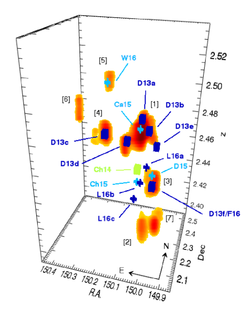
Figure 6: Same as Fig. 3, but in RA-Dec-z coordinates. Moreover, we overplot the location of the overdensity peaks/proto-clusters/proto-groups detected in other works in the literature (blue and green cubes, and blue and cyan crosses). Different colours and shapes are used for the symbols for clarity purposes only. Labels correspond to the IDs in Table 4. The dimensions of the symbols are arbitrary and do not refer to the extension of the overdensity peaks found in the literature.

Table 4: List of density peaks/proto-clusters/proto-groups already found in the literature. (1) ID of the proto-structures, as the labels in Fig. 6. (2) References: 1- Diener et al. (2015); 2- Casey et al. (2015); 3- Chiang et al. (2015); 4- Lee et al. (2016); 5- Wang et al. (2016); 6- Diener et al. (2013); 7- Chiang et al. (2014); 8-Franck & McGaugh (2016). (3), (4), (5), and (6) are the redshift, the overdensity value, the velocity dispersion and the total halo mass, taken from the corresponding paper, when available; in some cases, the redshift is the central redshift of the used redshift slice. When necessary, total masses from the literature are converted so as to correspond $h=0.70$. Column (7) is the volume of the overdensity peaks as described in their respective papers, while (8) and (9) are the average $\delta_{\rm gal}$ and total mass (computed with Eq. 1) as computed in our 3D data cube in the volume quoted in column (7). (10) matching peak of this work (see also the discussions in Sect. 4.2); the asterisks mark the cases when the match is not one-to-one, or there is a slight mis-match between the centres, and in these cases we quote our closest peak, as discussed in Sect. 4.2. Columns from (11) to (15) are average overdensity, volume, $M_{\rm tot}$, $\sigma_{\rm v}$ and $M_{\rm vir}$ of the matching peak in this work (see Tables 1 and 3) in the cases of a clear match. Notes: ^a The overdensity is computed using LAE galaxies. ^b The three subcomponents L16a, L16b and L16c are treated together as one single proto-cluster by Lee et al. (2016) when they compute the total mass, so the quoted number is the overall mass comprising the three components, for both the values in their paper (column 6) and as recovered in this work (columns 7, 8 and 9). ^c The overdensity is computed using DSFG galaxies. ^d The first mass is the overdensity mass, the second the virial mass. ^e For the sake of clarity, we omit the uncertainties, which are already reported in the previous tables.

Literature						From this work
ID	Ref.	z	$\delta_{\rm gal}$	$\sigma_{\rm v}$	Mtot	Volume	$\langle\delta_{\rm gal}\rangle$	Mtot	Match with	$\langle\delta_{\rm gal}\rangle$	Volume	Mtote	$\sigma_{\rm v}$e	Mvire
(Fig. 6)				[km s-1]	[$10^{14}$ M⊙]	cMpc3		[$10^{14}$ M⊙]	this work		cMpc3	[$10^{14}$ M⊙]	[km s-1]	[$10^{14}$ M⊙]
(1)	(2)	(3)	(4)	(5)	(6)	(7)	(8)	(9)	(10)	(11)	(12)	(13)	(14)	(15)
L16a	4	2.450	-	-	1.6$\pm$0.9b	1568b	1.50b	0.83b	[3]*	-	-	-	-	-
L16b	4	2.443	-	-	1.6$\pm$0.9b	1568b	1.50b	0.83b	[3]*	-	-	-	-	-
L16c	4	2.435	-	-	1.6$\pm$0.9b	1568b	1.50b	0.83b	[3]*	-	-	-	-	-
W16	5	2.506	-	530$\pm 120$	0.79${}^{+0.46}_{-0.29}$	429	2.46	0.29	[5]	3.11	252	0.190	533	0.82
F16	8	2.442	9.27$\pm$4.93	770	15.5/14.1d	$\sim 10000$	1.04	4.89	[3]	3.03	805	0.598	417	0.41
D15	1	2.450	10	426	-	1513	1.99	0.92	[3]	3.03	805	0.598	417	0.41
Ca15	2	2.472	11c	-	$>0.8\pm 0.3$	8839	1.55	4.82	[1]	3.79	3134	2.648	731	2.16
Ch15	3	2.440	4a	-	-	$\sim 12000$	0.53	$\sim 5.6$	[3]*	-	-	-	-	-
Ch14	7	2.450	1.34${}^{+0.49}_{-0.40}$	-	-	$\sim 23000$	0.37	$\sim 9.1$	[3]*	-	-	-	-	-
D13a	6	2.476	-	264	-	87	3.12	0.07	[1]*	-	-	-	-	-
D13b	6	2.469	-	488	-	253	3.73	0.21	[1]*	-	-	-	-	-
D13c	6	2.469	-	239	-	108	4.26	0.10	[4]	3.20	720	0.552	672	1.68
D13d	6	2.463	-	30	-	26	4.08	0.02	[1]*	-	-	-	-	-
D13e	6	2.452	-	476	-	38	0.89	0.02	[1]*	-	-	-	-	-
D13f	6	2.440	-	526	-	425	2.87	0.31	[3]	3.03	805	0.598	417	0.41

5 Discussion

The detection of such a huge, massive structure, caught during its formation, poses challenging questions. On the one hand, one would like to know whether we can predict the evolution of its components. On the other, it would be interesting to understand whether at least some of these components are going to interact with one another, or at the very least, how much they are going to interact with the surrounding large-scale structure as a whole. Moreover, the existence of superclusters at lower redshifts begs the question of whether this proto-structure will evolve to become similar to one of these closer superclusters. We address these issues below in a qualitative way, and defer any further analysis to a future work.

5.1 The evolution of the individual density peaks.

Assuming the framework of the spherical collapse model, we computed the evolution of our overdensity peaks as if they were isolated spherical overdensities. This is clearly a significant assumption (see e.g. Despali et al. 2013 for the evolution of ellipsoidal halos), but it can help us in roughly understanding the evolutionary status of these peaks, and how peaks with similar overdensities would evolve with time.

According to the spherical collapse model, any spherical overdensity will evolve like a sub-universe, with a matter-energy density higher than the critical overdensity at any given epoch. In our case, we reasonably assume that the average matter overdensity $\langle\delta_{\rm m}\rangle$ in our peaks corresponds to a non-linear regime, because it is already well above 1. We report $\langle\delta_{\rm m}\rangle$ in Table 5 as $\langle\delta_{\rm m,corr}\rangle$, given that we define it as $\langle\delta_{\rm m,corr}\rangle=\langle\delta_{\rm gal,corr}\rangle/b$, with $\langle\delta_{\rm gal,corr}\rangle$ as reported in Table 2 and $b$ the bias measured by Durkalec et al. (2015) as in Sect. 3.2.

Given that it is much easier to compute the evolution of an overdensity in linear regime than in non-linear regime, we transform (Padmanabhan 1993) our $\langle\delta_{\rm NL}\rangle$ into their corresponding values in linear regime, $\langle\delta_{\rm L}\rangle$, and make them evolve according to the spherical linear collapse model.

In particular, the overdense sphere passes through three specific evolutionary steps. The first one is the point of turn-around, when the overdense sphere stops expanding and starts collapsing, becoming a gravitationally bound structure. This happens when the overdensity in linear regime is $\delta_{\rm L,ta}\simeq 1.062$ (in non-linear regime it would be $\delta_{\rm NL,ta}\simeq 4.55$). After the turn-around, when the radius of the sphere becomes half of the radius at turn-around, the overdense sphere reaches the virialisation. In this moment, we have $\delta_{\rm L,vir}\simeq 1.58$ and $\delta_{\rm NL,vir}\simeq 146$. The sphere then continues the collapse process, till the moment of maximum collapse which theoretically happens when its radius becomes zero with an infinite density. In the real universe the collapse stops before the density becomes infinite, and at that time the system, which still satisfies the virial theorem, reaches $\delta_{\rm L,c}\simeq 1.686$ ($\delta_{\rm NL,c}\simeq 178$).

In our work we are interested in the moments of turn-around and collapse. Here we will follow the formalism as in Pace et al. (2010), and we will use the symbol $\delta_{\rm c}$ for $\delta_{\rm L,c}\simeq 1.686$ and the symbol $\Delta_{\rm V}$ for $\delta_{\rm NL,c}\simeq 178$. When we refer to the time(/redshift) of turn-around and collapse, we use $t_{\rm ta}$(/$z_{\rm ta}$) and $t_{\rm c}$(/$z_{\rm c}$).

We reiterate that $\delta_{\rm c}$ and $\Delta_{\rm V}$ are constant with redshift in an Einstein - de Sitter (EdS) Universe, while they evolve with time in a $\Lambda$CDM cosmology, and their evolution depends on the relative contribution of $\Omega_{\rm\Lambda}(z)$ and $\Omega_{\rm m}(z)$ to $\Omega_{\rm tot}(z)$. At high redshift (e.g. $z=5$) when $\Omega_{\rm\Lambda}(z)$ is small, $\delta_{\rm c}$ and $\Delta_{\rm V}$ are close to their EdS counterparts. As time goes by, $\Omega_{\rm\Lambda}(z)$ increases and both $\delta_{\rm c}$ and $\Delta_{\rm V}$ decrease. This is shown, for instance, in Pace et al. (2010), where they show that $\delta_{\rm c}$ decreases by less than 1% from $z=5$ to $z=0$, while in the same timescale $\Delta_{\rm V}$ decreases from $\sim 178$ to $\sim 100$ (see also Bryan & Norman 1998, where they use the symbol $\Delta_{\rm c}$ instead of $\Delta_{\rm V}$). In our work we allow our overdensities to evolve in the linear regime, so we are interested at the time when they reach $\delta_{\rm c}$. Given its small evolution with redshift, we consider it a constant, set as in the EdS universe.

The evolution of a fluctuation is given by its growing mode $D_{\rm+}(z)$. At a given redshift $z_{\rm 2}$, the overdensity $\delta_{\rm L}(z_{\rm 2})$ can be computed knowing the overdensity at another redshift $z_{\rm 1}$ and the value of the growing mode at the two redshifts, as follows:

$$\delta_{\rm L}(z_{\rm 2})=\delta_{\rm L}(z_{\rm 1})\frac{D_{\rm+}(z_{\rm 2})}{D_{\rm+}(z_{\rm 1})}.$$ (7)

In a $\Lambda$CDM universe, we define the linear growth factor $g$ as $g\equiv D_{\rm+}(z)/a$, where $a=(1+z)^{-1}$ is the cosmic scale factor. By using an approximate expression for $g$ (see e.g. Carroll et al. 1992 and Hamilton 2001), which depends on $\Omega_{\rm\Lambda}(z)$ and $\Omega_{\rm m}(z)$, we can recover $D_{\rm+}(z)$ and with equation 7 derive the time when our peaks reach $\delta_{\rm L,ta}$ and $\delta_{\rm c}$, starting from the measured values of $\delta_{\rm L}(z_{\rm obs})$, with $z_{\rm obs}$ being the redshifts given in Table 1. Figure 7 shows the evolution of the density contrast of our peaks. In Table 5 we list the values of $z_{\rm ta}$ and $z_{\rm c}$, together with the time elapsed from $z_{\rm obs}$ to these two redshifts. As a very rough comparison, if we considered the entire Hyperion proto-supercluster with its $\langle\delta_{\rm gal}\rangle\sim 1.24$ (Sect. 3.2), and assumed an elongation equal to the average elongation of the peaks to derive its $\langle\delta_{\rm gal,corr}\rangle$ and then its $\langle\delta_{\rm m,corr}\rangle$, the proto-supercluster would have $\delta_{\rm L}\lesssim 0.8$ at $z=2.46$ (to be compared with the y-axis of Fig. 7).

We note that the evolutionary status of the peaks depends by definition on their average density, that is, the higher the density, the more evolved the overdensity perturbation. The most evolved is peak [6], which has $\langle\delta_{\rm m,corr}\rangle=12.66$, almost twice as large as the second densest peak (peak [5]). According to the spherical collapse model, peak [6] will be a virialised system by $z\sim 1.7$, that is, in $1.3$ Gyr from the epoch of observation. The least evolved is peak [2], that will take 0.6 Gyr to reach the turn-around and then another $\sim 3.8$ Gyr to virialise.

This simple exercise, which is based on a strong assumption, shows that the peaks are possibly at different stages of their evolution, and will become virialised structures at very different times. In reality, the peaks’ evolution will be more complex, given that they will possibly accrete mass/subcomponents/galaxies during their lifetimes, and these results make it desirable to study how we can combine the density-driven evolution of the individual peaks with the overall evolution of the Hyperion proto-supercluster as a whole. Moreover, by comparing the evolutionary status of each peak with the average properties of its member galaxies, it will be possible to study the co-evolution of galaxies and the environment in which they reside. We defer these analyses to future works.

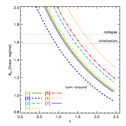
Figure 7: Evolution of $\delta_{m}$ for the seven peaks listed in Table 5, with different line styles as in the legend. The evolution is computed in a linear regime for a $\Lambda$CDM Universe. For each peak, we start tracking the evolution from the redshift of observation (column 2 in Table 5), and we consider as starting $\delta_{\rm m}$ the one computed from the corrected $\langle\delta_{\rm gal,corr}\rangle$ (column 7 in Table 2) and transformed into linear regime. The horizontal lines represent $\delta_{\rm L,ta}\simeq 1.062$, $\delta_{\rm L,vir}\simeq 1.58$ and $\delta_{\rm L,c}\simeq 1.686$. See Sect. 5.1 for more details.

Table 5: Evolution of the density peaks according to the spherical collapse model in linear regime. Columns (1) and (2) are the ID and the redshift of the peak, as in Table 2. Column (3) is the average matter overdensity derived from the average galaxy overdensity of column (7) of Table 2. Columns (4) and (5) are the redshifts when the overdensity reaches the overdensity of turn-around and collapse, respectively. Columns (6) and (7) are the corresponding time intervals $\Delta t$ since the redshift of observation $z_{\rm obs}$ (column 2) to the redshifts of turn-around and collapse. When $z_{\rm ta}<z_{\rm obs}$ the turn-around has already been reached before the redshift of observation, and in these cases the corresponding $\Delta t$ have not been computed. See Sect. 5.1 for more details.

ID	$z$	$\langle\delta_{\rm m,corr}\rangle$	$z_{\rm ta}$	$z_{\rm c}$	$\Delta t_{\rm ta}$	$\Delta t_{\rm c}$
					[Gyr]	[Gyr]
(1)	(2)	(3)	(4)	(5)	(6)	(7)
1	2.468	4.25	2.402	1.054	0.08	3.16
2	2.426	2.04	2.001	0.781	0.60	4.37
3	2.444	6.24	$>z_{\rm obs}$	1.282	-	2.32
4	2.469	4.60	$>z_{\rm obs}$	1.108	-	2.95
5	2.507	6.94	$>z_{\rm obs}$	1.388	-	2.07
6	2.492	12.66	$>z_{\rm obs}$	1.675	-	1.33
7	2.423	4.21	2.347	1.017	0.10	3.26

5.2 The proto-supercluster as a whole.

In the previous section we pretended that the peaks were isolated density fluctuations and traced their evolution in the absence of interactions with other components of the proto-supercluster. This is an oversimplification, because several kinds of interactions are likely to happen in such a large structure, such as for example accretion of smaller groups along filaments onto the most dense peaks, as expected in a $\Lambda$CDM universe.

For instance, for what concerns merger events between proto-clusters, Lee et al. (2016) examined the merger trees of some of the density peaks that they identified in realistic mock data sets by applying the same 3D Ly$\alpha$ forest tomographic mapping that they applied to the COSMOS field. They found that in the examined mocks, very few of the proto-structures identified by the tomography at $z\sim 2.4$ and with an elongated shape (such as the ‘chain’ of their peaks L16a, L16b, and L16c discussed in Sect. 4.2.3) are going to collapse to one single cluster at z=0. Similarly, Topping et al. (2018) analysed the Small MultiDark Planck Simulation in search for $z\sim 3$ massive proto-clusters with a double peak in the galaxy velocity distribution and with the two peaks separated by about $2000\,{\rm km\,s}^{-1}$, like the one they identified in previous observations (Topping et al. 2016). They found that such double-peaked overdensities are not going to merge into a single cluster at $z=0$.

The structures found by Lee et al. (2016) and Topping et al. (2016) are much smaller and with simpler shapes compared to the Hyperion proto-supercluster, and yet they are unlikely to form a single cluster at z=0, according to simulations. Interestingly, Topping et al. (2018) also found that in their simulation the presence of two massive peaks separated by $2000\,{\rm km\,s}^{-1}$ is a very rare event (one in $7.4h^{3}$Gpc^-3) at $z\sim 3$. These findings indicate that the evolution of the Hyperion proto-supercluster cannot be simplified as series of merging events, and that the identification of massive/complex proto-clusters at high redshift could be useful to give constraints on dark matter simulations.

Indeed, it would be interesting to know whether or not Hyperion could be the progenitor of known lower-redshift superclusters. One difficulty is that there is no unique definition of a supercluster (but see e.g. Chon et al. 2015 for an attempt), and the taxonomy of known superclusters up to $z\sim 1.3$ spans wide ranges of mass (from a few $10^{14}M_{\odot}$ as in Swinbank et al. 2007 to $>10^{16}M_{\odot}$ as in Bagchi et al. 2017), dimension (a few cMpc as in Rosati et al. 1999 or $\sim 100$ cMpc as in Kim et al. 2016), morphology (compact as in Gilbank et al. 2008, or with multiple overdensities as in Lubin et al. 2000; Lemaux et al. 2012), and evolutionary status (embedding collapsing cores as in Einasto et al. 2016 or already virialised clusters as in Rumbaugh et al. 2018). This holds also for the well-known superclusters in the local universe (see e.g. Shapley & Ames 1930; Shapley 1934; de Lapparent et al. 1986; Haynes & Giovanelli 1986), not to mention the category of the so-called Great Walls, which are sometimes defined as systems of superclusters (like e.g. the Sloan Great Wall, Vogeley et al. 2004; Gott et al. 2005, and the Boss Great Wall, Lietzen et al. 2016).

Clearly, Hyperion shares many characteristics with the above-mentioned superclusters, making it likely that its eventual fate will be to become a supercluster. A further step would be identifying which known supercluster is most likely to be similar to the potential descendant(s) of Hyperion. This would be surely an important step in understanding how the large-scale structure of the universe evolves and how it affects galaxy evolution. On the other hand, it is also interesting to study the likelihood of such (proto-) superclusters existing in a given cosmological volume, given their volumes and masses (see e.g. Sheth & Diaferio 2011). For instance, Lim & Lee (2014) show that the relative abundance of rich superclusters at a given epoch could be used as a powerful cosmological probe.

From Lim & Lee (2014) we can qualitatively assess how many superclusters of the kind that we detect are expected in the volume probed by VUDS. Lim & Lee (2014) derive the mass function of superclusters, defined as clusters of clusters according to a Friend of Friend algorithm. Since the supercluster mass function at $z\sim 2.5$ was not explicitly studied, we adopt here expectations from their study of the $z=1$ supercluster mass function keeping in mind that this expectation will be a severe upper limit given that the halo mass function at the high-mass end decreases by a factor of $\ga 100$ from $z=1$ to $z=2.5$ (see, e.g. Percival 2005). With this in mind, we estimate, using those results of Lim & Lee (2014) that employ a similar cosmology to the one used in this study, the extreme upper limit to the number of superclusters with a total mass $>5\times 10^{14}$ M_⊙ expected within the RA-Dec area studied in this paper and in the redshift range $2<z<4$ to be $\sim$4. We consider this mass limit, $>5\times 10^{14}$ M_⊙, because it is the sum of the masses of our peaks, similarly to how they compute the masses of their superclusters. The extremeness of this upper limit is such that much more precise comparisons need to be made. We defer the detailed analysis of number counts and evolution of proto-superclusters at $z\sim 2.5$ in simulated cosmological volumes to a future work.

6 Summary and conclusions

Thanks to the spectroscopic redshifts of VUDS, together with the zCOSMOS-Deep spectroscopic sample, we unveiled the complex shape of a proto-supercluster at $z\sim 2.45$ in the COSMOS field. We computed the 3D overdensity field over a volume of $\sim 100\times 100\times 250$ comoving Mpc³ by applying a Voronoi tessellation technique in overlapping redshift slices. The tracers catalogue comprises our spectroscopic sample complemented by photometric redshifts for the galaxies without spectroscopic redshift. Both spectroscopic and photometric redshifts were treated statistically, according to their quality flag or their measurement error, respectively. The main advantage of the Voronoi Tessellation is that the local density is measured both on an adaptive scale and with an adaptive filter shape, allowing us to follow the natural distribution of tracers. In the explored volume, we identified a proto-supercluster, dubbed “Hyperion” for its immense size and mass, extended over a volume of $\sim 60\times 60\times 150$ comoving Mpc³. We estimated its total mass to be $\sim 4.8\times 10^{15}{\rm M}_{\odot}$. Within this immensely complex structure, we identified seven density peaks in the range $2.40<z<2.5$, connected by filaments that exceed the average density of the volume. We analysed the properties of the peaks, as follows:

• We estimated the total mass of the individual peaks, $M_{\rm tot}$, based on their average galaxy density, and found a range of masses from $\sim 0.1\times 10^{14}{\rm M}_{\odot}$ to $\sim 2.7\times 10^{14}{\rm M}_{\odot}$.

• By assigning spectroscopic members to each peak, we estimated the velocity dispersion of the galaxies in the peaks, and then their virial mass $M_{\rm vir}$ (under the admittedly strong assumption that they are virialised). The agreement between $M_{\rm vir}$ and $M_{\rm tot}$ is surprisingly good, considering that (almost all) the peaks are most probably not yet virialised.

• If we assume that the peaks are going to evolve separately, without accretion/merger events, the spherical collapse model predicts that these peaks have already started or are about to start their collapse phase (‘turn-around’), and they will all be virialised by redshift $z\sim 0.8$.

• We finally performed a careful comparison with the literature, given that some smaller components of this proto-supercluster had previously been identified in other works using heterogeneous galaxy samples (LAEs, 3D Ly$\alpha$ forest tomography, sub-mm starbursting galaxies, CO emitting galaxies). In some cases we found a one-to-one match between previous findings and our peaks, in other cases the match is disputable. We note that a direct comparison is often difficult because of the different methods/filters used to identify proto-clusters.

In summary, with VUDS we obtained, for the first time across the central $\sim 1$ deg² of the COSMOS field, a panoramic view of this large structure that encompasses, connects, and considerably expands on all previous detections of the various sub-components. The characteristics of the Hyperion proto-supercluster (its redshift, its richness over a large volume, the clear detection of its sub-components), together with the extensive band coverage granted by the COSMOS field, provide us the unique possibility to study a rich supercluster in formation 11 billion years ago.

This impressive structure deserves a more detailed analysis. On the one hand, it would be interesting to compare its mass and volume with similar findings in simulations, because the relative abundance of superclusters could be used to probe deviations from the predictions of the standard $\Lambda$CDM model. On the other hand, it is crucial to obtain a more complete census of the galaxies residing in the proto-supercluster and its surroundings. With this new data, it would be possible to study the co-evolution of galaxies and the environment in which they reside, at an epoch ($z\sim 2-2.5$) when galaxies are peaking in their star-formation activity.

Appendix A Stability of the peaks properties

We investigated the extent to which the choice of a 5$\sigma_{\delta}$ threshold affects some of the properties of the identified peaks. Namely, we varied the overdensity threshold from 4.5$\sigma_{\delta}$ to 5.5$\sigma_{\delta}$, and verified the variation of $M_{\rm tot}$ (Table 1), velocity dispersion (Table 3) and elongation (Table 2) as a function of the used threshold.

A.1 Total mass

Figure 8 shows the fractional variation of $M_{\rm tot}$ (Table 1) as a function of the adopted threshold, which is expressed in terms of the corresponding multiple of $\sigma_{\delta}$. Five peaks out of seven show roughly the same variation, while peak [1] has a much smaller variation and peak [7] a much steeper one. This might imply that the (baryonic) matter distribution within peak [7] is less peaked toward the centre with respect to the other peaks, while the matter distribution within peak [1] is more peaked.

Given that we are probing very dense peaks (they are about to collapse, see Sect. 5), we expect the total mass enclosed above a given overdensity threshold to have large variations if we vary the overdensity threshold by much. If instead we focus on a small $n_{\sigma}$ range around our nominal value of $n_{\sigma}=5$, for instance the interval $5\pm 0.2$, we see that the variation of the total mass is much smaller than the uncertainty on the total mass quoted in Table 1, which was computed by using the density maps obtained with $\delta_{\rm gal,16}$ and $\delta_{\rm gal,84}$ (see Sect. 3.1).

This means that, although the total mass of our peaks depends on the chosen overdensity threshold, because of the very nature of the mass distribution in these peaks, at the chosen threshold the uncertainty is dominated by the uncertainty on the reconstruction of the density field and not by our precise definition of ‘overdensity peak’.

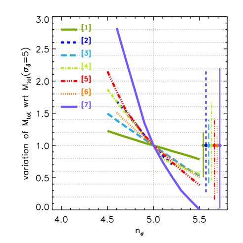
Figure 8: Fractional variation of the total mass $M_{\rm tot}$ (Table 1) for the seven peaks as a function of the overdensity threshold adopted to identify them, expressed in terms of the corresponding multiples $n_{\sigma}$ of $\sigma_{\delta}$. The reference total mass value is the one at the 5$\sigma_{\delta}$ threshold. The different lines correspond to the different peaks as in the legend. The filled symbols on the right, with their error bars, correspond to the fractional variation of $M_{\rm tot}$ calculate at $5\sigma_{\delta}$ resulting from the uncertainties on the density reconstruction quoted in Table 1. The position of the error bars on the x-axis is arbitrary. In all cases, these errors are much larger than the uncertainty resulting from slightly modulating the overdensity threshold employed.

A.2 Velocity dispersion

Similarly to the variation of the total mass, we verified how the velocity dispersion $\sigma_{\rm v}$ varies as a function of the adopted overdensity threshold, for the seven identified peaks. For each threshold, the velocity dispersion and its error are computed as described in Sect. 4.1, and only when we could use at least three spectroscopic galaxies. For all the peaks, $\sigma_{\rm v}$ is relatively stable in the entire range of the explored overdensity thresholds, and its small variations (due to the increasing or decreasing number of spectroscopic members) are always much smaller than the uncertainties computed on the velocity dispersion itself, at fixed $n_{\sigma}$. For this reason we consider the virial masses quoted in Table 3 to be independent from small variations of the overdensity threshold.

We remind the reader that for the computation of the velocity dispersion we used a more relaxed definition of galaxy membership within each peak so as to increase the number of the available galaxies (see Sect. 4.1). Even with this broader definition, for peak [7] we had only two galaxies available if we used $n_{\sigma}=5$ to define the peak, while their number increased to four by using $n_{\sigma}=4.9$. For this reason, we decided that the most reliable value of $\sigma_{\rm v}$ for peak [7] is the one computed using $n_{\sigma}=4.9$, and we quote this $\sigma_{\rm v}$ in Table 3.

A.3 Elongation

Here we approximately estimate how the elongation depends on the typical dimension of our density peaks. Our estimation is based on the following simplistic assumptions: 1) the intrinsic shape of a proto-cluster is a sphere with radius $r_{\rm int}$, and its measured dimensions on the $x-$ and $y-$axis ($r_{x}$ and $r_{y}$) correspond to the intrinsic dimension $r_{int}$, i.e. $r_{x}=r_{y}=r_{\rm int}$, and 2) the measured dimension on the $z-$axis ($r_{z}$) corresponds to $r_{int}$ plus a constant factor $\Delta r$, which is the result of the complex interaction among the several factors that might cause the elongation (the depth of the redshift slices, the photometric redshift error etc), i.e. $r_{z}=r_{int}+\Delta r$. From these assumptions it follows:

$$\frac{r_{z}}{r_{xy}}=1+\frac{\Delta r}{r_{int}},$$ (8)

where $r_{xy}$ is the average between $r_{x}$ and $r_{y}$, and in our example we have $r_{xy}=r_{x}=r_{y}=r_{\rm int}$. If we substitute $r_{x}$, $r_{y}$ and $r_{z}$ with $R_{e,x}$, $R_{e,y}$ and $R_{e,z}$ as defined in Sect. 4, from Eq. 8 follows:

$$E_{\rm z/xy}=1+\frac{\Delta r}{R_{e,xy}},$$ (9)

with $E_{\rm z/xy}$ and $R_{e,xy}$ as defined in Sect. 4. This means that the measured elongation depends on the circularised 2D effective radius as $y=1+A/x$.

To verify this dependence, we measured $E_{\rm z/xy}$ and $R_{e,xy}$ for our seven peaks for different thresholds, expressed in terms of the multiples $n_{\sigma}$ of $\sigma_{\rm\delta}$. In this case, we made the threshold vary from 4.1 to 7 $\sigma_{\rm\delta}$, because the two peaks [1] and [4] merge in one huge structure if we use a threshold $<4.1\sigma_{\delta}$. We notice that peak [5] disappears for $\sigma_{\rm\delta}>5.8$ above the mean density, and peak [7] for $\sigma_{\rm\delta}>5.4$. The peaks [1], [2] and [4] are split into two smaller peaks when $\delta_{\rm gal}$ is above 6.5$\sigma_{\rm\delta}$, 5.2$\sigma_{\rm\delta}$ and 5.1$\sigma_{\rm\delta}$ above the mean density, respectively. Figure 9 shows how $E_{\rm z/xy}$ varies as a function of $R_{e,xy}$. The three curves with equation $y=1+A/x$ are shown to guide the eye, with $A$ tuned by eye to match the normalisation of some of the observed trends. It is evident that the foreseen dependence of $E_{\rm z/xy}$ on $R_{e,xy}$ is confirmed. In the Figure, $A$ increases by a factor of $\sim 3$ from the lowest curve (corresponding e.g. to peak [7]) to the highest one (matching e.g. peak [6]). The specific value of $A$ is likely due to a complex combination of peculiar velocities, spectral sampling, reconstruction methods (e.g. slice size relative to the true l.o.s. extent), and photometric redshift errors. It is beyond the scope of this paper to precisely quantify the contribution of each for each individual peak. Nevertheless, although in some cases $E_{\rm z/xy}$ quickly vary for small changes of $R_{e,xy}$ (i.e. small changes in the threshold), this plot confirms that its measured values are reasonably consistent with our expectations.

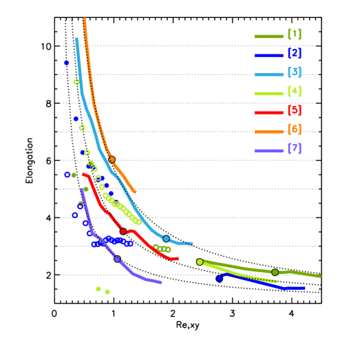
Figure 9: Elongation $E_{\rm z/xy}$ as a function of $R_{e,xy}$. The different colours refer to the different peaks as in the legend. $E_{\rm z/xy}$ and $R_{e,xy}$ are measured by fixing different thresholds (number of $\sigma_{\rm\delta}$ above the mean density) to define the peaks themselves, ranging from 4.1 to 7 $\sigma_{\rm\delta}$. $E_{\rm z/xy}$ and $R_{e,xy}$ measured at the $5\sigma_{\rm\delta}$ threshold are highlighted with a filled circle, and are the same quoted in Table 2. The peaks [1] and [2] are split into two smaller peaks when $\delta_{\rm gal}$ is above 5.5$\sigma_{\rm\delta}$ and 5.7$\sigma_{\rm\delta}$ above the mean density, respectively: this is shown in the plot by splitting the curve of the two peaks into two series of circles (filled and empty). The three dotted lines corresponds to the curves $y=1+A/x$, with $A=4.3,2.9,1.5$ from top to bottom. The values of A are chosen to make the curves overlap with some of the data, to guide the eye.

Appendix B Details on individual peaks

We show here the projections on the RA-Dec and $z$-Dec planes of the four most massive peaks (“Theia”, “Eos”, “Helios”, and “Selene”), to highlight their complex shape. The remaining peaks have very regular shapes on the RA-Dec and $z$-Dec planes, so we do not show them here. The projections that we show include the peak isodensity contours in the 3D cube and the position of the spectroscopic member galaxies. The $z$-Dec projection is associated to the velocity distribution of the spectroscopic members.