Self-contained two-layer shallow-water theory
of strong internal bores

Abstract

We show that interfacial gravity waves comprising strong hydraulic jumps (bores) can be described by a two-layer hydrostatic shallow-water (SW) approximation without invoking additional front conditions. The theory is based on a new SW momentum equation which is derived in locally conservative form containing a free parameter $\alpha.$ This parameter, which defines the relative contribution of each layer to the pressure at the interface, affects only hydraulic jumps but not continuous waves. The Rankine-Hugoniot jump conditions for the momentum and mass conservation equations are found to be mathematically equivalent to the classical front conditions, which were previously thought to be outside the scope of SW approximation. Dimensional arguments suggest that $\alpha$ depends on the density ratio. For nearly equal densities, both layers are expected to affect interfacial pressure with approximately equal weight coefficients, which corresponds to $\alpha\approx 0.$ The front propagation velocity for $\alpha=0$ agrees well with experimental and numerical results in a wide range of bore strengths. A remarkably better agreement with high-accuracy numerical results is achieved by $\alpha=\sqrt{5}-2,$ which yields the largest height that a stable gravity current can have.

¹Fluid and Complex Systems Research Centre, Coventry University,
Coventry, CV1 5FB, United Kingdom
² Department of Physics, University of Latvia, Riga, LV-1004, Latvia

1 Introduction

Shallow-water (SW) approximation is commonly used in the geophysical fluid dynamics to model ocean currents and large-scale atmosphere circulation [42]. Because such flows are typically dominated by inertia and have a horizontal length scale much larger than the characteristic depth, they can be treated as effectively horizontal and vertically invariant. This simplifies the hydrodynamic problem from three to two spatial dimensions, thus essentially reducing computational complexity of such flows. The SW approximation can also be used for modeling long gravity waves on the liquid surfaces or interfaces in stably stratified fluid layers. The latter type of systems are not only routinely used as simplified models of internal waves in oceans [24] but are also encountered in technological applications like aluminum reduction cells [20] and the recently developed liquid metal batteries [28].

In the commonly used hydrostatic SW approximation, waves are known to become steeper with time and to develop vertical fronts analogous to the shock waves in the gas dynamics [18]. In the fluid dynamics, such shocks are called hydraulic jumps or bores [48] – both terms are used interchangeably here. Hydraulic jumps can also be present initially, for example, when fluid starts to flow by breaking a dam or when a lock separating two liquids with different densities is opened [19]. Mathematically, hydraulic jumps appear as discontinuities in the wave amplitude. Physically, they encapsulate smooth variations of the flow field over the length scales comparable to the layer depth.

It is commonly assumed that although the partial differential equations (PDEs) which govern the wave propagation cease to apply at the discontinuities, the relevant physics, which is represented by the conservation laws behind those equations, may still hold [51]. Thus, the propagation of hydraulic jumps is expected to be governed not by the original PDEs but by equivalent integral relationships which are known as the Rankine-Hugoniot conditions in the gas dynamics. Such relationships can be obtained for the PDEs of the form

$$\partial_{t}P(\boldsymbol{u})+\partial_{x}Q(\boldsymbol{u})=0$$

by integrating them across the discontinuity. This type of equation represents a local conservation law for the quantity $P$ with the flux $Q$ and the dynamical variables $\boldsymbol{u}(x,t).$ Conservation laws determine the speed at which a jump propagates without using any information about the flow inside the jump.

For a single fluid layer, there is an infinite number of such conservation laws [51, p. 459]. For a two-layer system with a free surface, only six such linearly independent laws exist [41, 38, 7]. For a two-layer system bounded by a rigid lid, an infinite number of conservation laws is expected [41, 37]. However, only three most elementary laws, which describe the conservation of mass, irrotationality (zero vorticity) and energy are generally known. No local momentum conservation law appears to be known in this case. At the same time, the conservation of momentum is known to play a key role for the hydraulic jumps in single fluid layers. At the same time, single layer represents the limiting case of a two-layer system when either the density of the top layer or the depth of the bottom layer becomes small [48].

The lack of a local momentum conservation law has led to the assumption that two-layer SW equations are inherently non-conservative [2] and unable to describe internal hydraulic jumps without additional closure relations. The latter are usually deduced by dimensional arguments [1] or derived using various semi-empirical integral models [5]. For gravity currents, which are created when a layer of heavier liquid is driven by its weight along the bottom into a lighter ambient fluid, such a front condition relating the velocity of propagation with the depth of the layer is the central result of the celebrated Benjamin’s theory [8]. This hydraulic-type condition and its various empirical extensions [30, 25] are commonly regarded as essential for the numerical modeling of gravity currents using the hydrostatic SW approximation [49, 45].

A number of similar semi-empirical front conditions have been proposed also for internal bores [54, 4, 53, 31]. Despite the long history of this problem, there is still no comprehensive theoretical description of internal bores, and new models and front conditions continue to emerge [12, 11, 6, 50, 21] motivated by the importance such bores play in various geophysical flows ranging from coastal oceans [47] to the inversion layers in the atmosphere [16].

In this paper, we propose a new SW theoretical framework for the analysis and numerical modeling of interfacial waves containing hydraulic jumps. In contrast to the previous SW models, no external front conditions are required in our model. The theory is based on a novel, locally conservative momentum equation, which is derived from the basic SW equations. The derived equation contains a free parameter $\alpha,$ which emerges due to the inherent non-uniqueness of the SW momentum equation for two-layer system of fixed height. The proposed SW framework is mathematically rigorous and free of phenomenological concepts like the head loss or energy dissipation in separate layers, which are fundamental to the conventional control-volume approach.

The paper is organized as follows. In the next section, we introduce a two-layer model and derive the SW equations in locally conservative form for fluids with significantly different as well as nearly equal densities. Jump conditions for the latter case are derived in section 3, where we also compare the resulting front speeds with the predictions of some previous models as well as with experimental and numerical data. In section 4, we consider bores which can form atop gravity currents and, thus, to connect the latter to deeper upstream states. The paper is concluded with section 5 where the main results are summarized and the principal differences between the SW and control-volume approaches are critically discussed. A more detailed discussion of the key differences between the proposed SW theory and two alternative approaches is presented in the Appendix.

2 Two-layer SW model

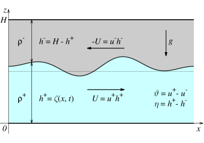
Figure 1: Sketch of the problem showing a horizontal channel of constant height $H$ bounded by two parallel solid walls and filled with two inviscid immiscible fluids with constant densities $\rho^{+}$ and $\rho^{-},$ where $h^{+}=\zeta(x,t)$ and $h^{-}=H-h^{+}$are the depths of the bottom and top layers, respectively.

Consider a horizontal channel of a constant height $H$ which is bounded by two parallel solid walls and filled with two inviscid immiscible fluids with constant densities $\rho^{+}$ and $\rho^{-}$ as shown in Fig. 1. The fluids are subject to a downward gravity force with the free fall acceleration $g.$ The interface separating the fluids at the horizontal position $x$ and the time instant $t$ is located at the height $z=\zeta(x,t).$ The latter is equal to the depth of the bottom layer $h^{+}=H-h^{-},$ where $h^{-}$ is the depth of the top layer. The velocity $\boldsymbol{u}^{\pm}$ and the pressure $p^{\pm}$ in each layer are governed by the Euler equation

$$\partial_{t}\boldsymbol{u}+\boldsymbol{u}\cdot\boldsymbol{\nabla}\boldsymbol{u}=-\rho^{-1}\boldsymbol{\nabla}p+\boldsymbol{g}$$ (1)

and the incompressibility constraint $\boldsymbol{\nabla}\cdot\boldsymbol{u}=0.$ Henceforth, for the sake of brevity, we drop $\pm$ indices wherever analogous expressions apply to both layers. At the interface $z=\zeta(x,t)$, we have the continuity of pressure, $[p]\equiv p^{+}-p^{-}=0,$ and the kinematic condition

$$w=\frac{d\zeta}{dt}=\zeta_{t}+u\zeta_{x},$$ (2)

where $u$ and $w$ are the $x$ and $z$ components of velocity, and the subscripts $t$ and $x$ stand for the corresponding partial derivatives. Integrating the incompressibility constraint over the depth of each layer and using Eq. (2), we obtain

$$h_{t}+(h\bar{u})_{x}=0,$$ (3)

where the overbar denotes the depth average. Similarly, averaging the horizontal $(x)$ component of Eq. (1), we have

$$(h\bar{u})_{t}+(h\overline{u^{2}})_{x}=-\rho^{-1}h\overline{p_{x}}.$$ (4)

Pressure follows from the integration of the vertical $(z)$ component of Eq. (1) as

$$p(x,z,t)=\mathit{\Pi}(x,t)+\rho\int_{\zeta}^{z}(w_{t}+\boldsymbol{u}\cdot\boldsymbol{\nabla}w-g)dz,$$ (5)

where the constant of integration $\mathit{\Pi}(x,t)=\left.p^{\pm}(x,z,t)\right|_{z=\zeta}$ defines the distribution of pressure along the interface. Averaging the $x$-component of the gradient of pressure (5) over the depth of each layer, after a few rearrangements, we obtain

$$\overline{p_{x}}=\left(\mathit{\Pi}+\rho g\zeta+\rho\overline{(z-z_{0})(w_{t}+\boldsymbol{u}\cdot\boldsymbol{\nabla}w)}\right)_{x},$$ (6)

which defines the RHS of Eq. (4) with $z_{0}=0$ and $z_{0}=H$ for the bottom and top layers, respectively.

In the SW approximation, which is applicable when the characteristic horizontal length scale $L$ is much larger than the height $H,$ i.e. $H/L=\epsilon\ll 1,$ the exact depth-averaged equations above can be simplified follows. In this case, the incompressibility constraint implies $w/u=O(\epsilon)$ and Eq. (6) correspondingly reduces to

$$\overline{p_{x}}=(\mathit{\Pi}+\rho g\zeta)_{x}+O(\epsilon^{2}),$$ (7)

where the leading-order term is purely hydrostatic and $O(\epsilon^{2})$ represents a small dynamical pressure correction due to the vertical velocity $w.$ Additionally, the flow in each layer is assumed to be irrotational: $\boldsymbol{\omega}=\boldsymbol{\nabla}\times\boldsymbol{u}=0.$ According to the inviscid vorticity equation

$$\frac{d\boldsymbol{\omega}}{dt}=(\boldsymbol{\omega}\cdot\boldsymbol{\nabla)}\boldsymbol{u,}$$

this property is preserved by Eq. (1). In the leading-order approximation, the irrotationality condition reduces to $\partial_{z}u^{(0)}=0$. It means that the horizontal velocity can be decomposed as

$$u=\bar{u}+\tilde{u},$$ (8)

where $\tilde{u}$ is the deviation from average which according to Eq. (7) is $O(\epsilon^{2}).$ Consequently, in the second term of Eq. (4), we have $\overline{u^{2}}=\bar{u}^{2}+O(\epsilon^{4}).$ Finally, using Eq. (3) and ignoring $O(\epsilon^{2})$ dynamic pressure correction, Eq. (4) can be written as

$$\rho(\bar{u}_{t}+\tfrac{1}{2}\text{$\bar{u}^{2}$}_{x}+g\zeta_{x})=-\mathit{\Pi}_{x}.$$ (9)

This and Eq. (3) constitute the basic set of SW equations in the leading-order (hydrostatic) approximation.

For completeness, note that the vertical velocity, which is outside the scope of the present study, can obtained from the incompressibility constraint and Eq. (8) as

$$w(z)=-\int_{z_{0}}^{z}u_{x}dz=-(z-z_{0})\bar{u}_{x}+O(\epsilon^{2}),$$ (10)

where $z_{0}$ is defined as in Eq. (6) to satisfy the impermeability conditions $w(0)=w(H)=0.$ Then Eq. (6) straightforwardly leads to the well-known result [22, 33, 15]

$$h\overline{p_{x}^{(1)}}=-\frac{1}{3}\rho\left(h^{3}(D_{t}\bar{u}_{x}-\text{$\bar{u}_{x}$}^{2}\right)_{x}+O(\epsilon^{4})=\frac{1}{3}\rho\left(h^{2}D_{t}^{2}h\right)_{x}+O(\epsilon^{4}),$$ (11)

where $D_{t}\equiv\partial_{t}+\bar{u}\partial_{x}$ and $\bar{u}_{x}=-h^{-1}D_{t}h.$ The latter relation follows from Eq. (3) and ensures that kinematic constraint (2) is satisfied by Eq. (10) up to $O(\epsilon^{2}).$

On one hand, the wave dispersion caused by the weakly non-hydrostatic pressure correction (11) can prevent the development of discontinuities and enable the formation of solitary waves and permanent-shape bores (solibores) [15]. On the other hand, the weakly non-hydrostatic approximation is limited to relatively shallow waves and, thus, inapplicable to strong internal bores [19]. The latter are the main focus of the present study, where we show that such bores can be described by the hydrostatic SW approximation in a self-contained way without invoking externally derived front conditions.

The system of four SW Eqs. (9) and (3) contains five unknowns: $u^{\pm}$, $h^{\pm}$ and $\mathit{\Pi},$ and is completed by adding the fixed height constraint $\{h\}\equiv h^{+}+h^{-}=H.$ Henceforth, we simplify the notation by omitting the bar over $u$ and use the curly brackets to denote the sum of the enclosed quantities. Two more unknowns can be eliminated as follows. Firstly, adding the mass conservation equations for each layer together and using $\{h\}_{t}\equiv 0,$ we obtain $\{uh\}=\Phi(t),$ which is the total flow rate. In this study, the channel is assumed to be laterally closed, which means $\Phi\equiv 0,$ and, thus, $u^{-}h^{-}=-u^{+}h^{+}.$ Secondly, the pressure gradient $\mathit{\Pi}_{x}$ can be eliminated by subtracting the two Eqs. (9) one from another. This leaves only two unknowns, $U\equiv u^{+}h^{+}$ and $h=h^{+},$ and two equations, which can be written in a locally conservative form as

$$\left(\left\{\rho/h\right\}U\right)_{t}+\left(\tfrac{1}{2}\left[\rho/h^{2}\right]U^{2}+g\left[\rho\right]h\right)_{x} =0,$$ (12)

$$h_{t}+U_{x} =0.$$ (13)

where the square brackets denote the difference of the enclosed quantities between the bottom and top layers: $\left[f\right]\equiv f^{+}-f^{-}.$ In this form, both equations can in principle be integrated across the discontinuity to obtain the corresponding jump conditions. But this, as it will be shown in the following, is not the only possible set of locally conservative SW equations.

The applicability of Eqs. (12) and (13) to strong bores depends on the conservation of the corresponding quantities not only in simple one-dimensional flows, which are described explicitly by these equations, but also in more complex three-dimensional turbulent flows, which usually occur in strong bores. The conservation of mass described by Eq. (13) in each layer is supposed to hold if fluids are immiscible. This is assumed in the present study but may not always be the case [37]. The quantity conserved in Eq. (12), which can be written as

$$\left\{\rho/h\right\}U=[\rho u]=\int_{H}\partial_{z}(\rho u)\,dz,$$

is related to the vorticity. Namely, in each layer separately, we have $\partial_{z}(\rho u)=\rho\omega,$ where $\omega=\partial_{z}u\equiv 0$ is the vorticity in the hydrostatic approximation. On the other hand, the quantity conserved in Eq. (12) is related to $\oint\rho\boldsymbol{u}\cdot d\boldsymbol{r}=\int_{\mathit{\Gamma}}[\rho u]dx,$ which represents circulation in the $(x,z)$-plane around a small segment $\mathit{\Gamma}$ of the vortex sheet made by the interface. It is important to note that the conservation of this quantity is limited to strictly two-dimensional flows which only advect the vorticity but do not generate it. This, however, is not the case in three-dimensional flows in which vorticity can be generated by stretching and twisting of vortices. It implies that the quantity whose conservation is described by Eq. (12) may not be conserved in strong bores. Also note that this quantity is not expected to be conserved in single fluid layers either. The quantity which is expected to be conserved across hydraulic jumps in single fluid layers with smooth bottom is the momentum [27]. Analogous quantity can be expected to be conserved also in two-layer system with flat top and bottom boundaries.

To obtain momentum equation for the two-layer system we multiply Eq. (9) for each layer with $h^{\pm}$ and add both equations together. Using Eq. (13) along with the fixed-height condition, after a few rearrangements, we have

$$[\rho]U_{t}+\left(\{\rho/h\}U^{2}+\tfrac{1}{2}g[\rho h^{2}]+H\mathit{\Pi}\right)_{x}=0,$$ (14)

where $[\rho]U\equiv\{\rho uh\}$ is the momentum density. In this form, the momentum conservation equation is non-local because it contains not only the dynamical variables $U$ and $h$ but also the interfacial pressure $\mathit{\Pi}$. The latter can be eliminated from Eq. (14) in two alternative ways. First, if we follow the same steps as in deriving Eq. (14), but before adding the two equations together divide them by $\rho^{\pm},$ we obtain

$$\mathit{\Pi}_{x}=-\{h/\rho\}^{-1}\left(\{h^{-1}\}U^{2}+gHh\right)_{x}.$$

Although substituting this expression into Eq. (14) we can eliminate $\mathit{\Pi}_{x},$ it does not render the resulting equation locally conservative. The problem is the non-local dependence of the pressure $\mathit{\Pi=\int\mathit{\Pi}_{x}}\thinspace dx$ on the dynamical variables $U$ and $h.$ But it does not mean that Eq. (14) is inherently non-local as it is commonly believed. The alternative approach which allows us to cast this equation into locally conservative form, is to take $\mathit{\Pi}_{x}$ directly from Eq. (9). But here we are faced with a dilemma as $\mathit{\Pi}_{x}$ can be taken either from the equation for the top or bottom layer [40]. Note that requiring Eq. (9) to yield the same $\mathit{\Pi}_{x}$ for both layers leads back to Eq. (12), which, as discussed above, describes the conservation of circulation. Therefore, the two expressions of $\mathit{\Pi}_{x}$ following from Eq. (9) are equivalent only if Eq. (12) is satisfied. But this, as shown in the following, is not in general possible.

We resolve this dilemma by taking a linear combination of the pressure gradients defined by Eqs. (9) for each layer with weight coefficients $(1\pm\alpha)/2,$ where $\alpha$ is an arbitrary constant defining the contribution of each layer to $\mathit{\Pi}_{x}.$ This results in

$$\mathit{\Pi}_{x}=-\tfrac{1}{2}\left(\left(\left[\rho/h\right]U\right)_{t}+\left(\tfrac{1}{2}\left\{\rho/h^{2}\right\}U^{2}+g\left\{\rho\right\}h\right)_{x}\right)-\tfrac{1}{2}\alpha\mathit{\Lambda},$$ (15)

where

$$\mathit{\Lambda}=\left(\left\{\rho/h\right\}U\right)_{t}+\left(\tfrac{1}{2}\left[\rho/h^{2}\right]U^{2}+g\left[\rho\right]h\right)_{x}$$ (16)

is the LHS of Eq. (12). As seen from the definition of weight coefficients above, $\mathit{\Lambda}$ represents the difference of $\mathit{\Pi}_{x}$ between the values defined by Eqs. (9) for the bottom and top layers. Note that with $\alpha=1$, $\mathit{\Pi}_{x}$ is determined solely by the top layer, whereas the opposite is the case with $\alpha=-1.$ In general, we can also have $|\alpha|>1$ as one weight coefficient may be negative while the other is greater than unity. If Eq. (12) is satisfied, i.e. $\mathit{\Lambda}=0$, the last term in Eq. (15) with $\alpha$ vanishes. Then substituting $\mathit{\Pi}_{x}$ from Eq. (15) into Eq. (14), we obtain

$$\left([\rho-\tfrac{1}{2}H\rho/h]U\right)_{t}+\left(\{\rho/h-\tfrac{1}{4}H\rho/h^{2}\}U^{2}+\tfrac{1}{4}g[\rho]\{h^{2}\}\right)_{x}=0,$$ (17)

which is the two-layer momentum equation (14) written in locally conservative form. Note that it is not the momentum $[\rho]U$ but rather the pseudo-momentum $[\rho-\tfrac{1}{2}H\rho/h]U,$ called the impulse by Benjamin [9], which emerges as a conserved quantity in this equation. It reflects the inconspicuous fact that it is the pseudo-momentum rather than the momentum which is actually conserved in the laterally closed two-layer system bounded by a rigid lid [10, 13]. Equation (17) is equivalent to Eq. (12) and can be reduced to the latter by using Eq. (13) provided that both $U$ and $h$ are differentiable at least once. This is obviously not so at the points where $U$ and $h$ are discontinuous. In this case, Eqs. (12) and (17) cannot in general be satisfied simultaneously. It means that we cannot assume $\mathit{\Lambda}=0$ when substituting $\mathit{\Pi}_{x}$ from Eq. (15) into Eq. (14). Thus, the term $-\tfrac{1}{2}\alpha H\mathit{\Lambda}$ has to be retained in Eq. (17) for this equation to be applicable also to discontinuous solutions. Since Eq. (16) defining $\mathit{\Lambda}$ is locally conservative, so is also the momentum equation containing the extra term with $\alpha\mathit{\Lambda}:$

$$\left(\left([\rho-\tfrac{1}{2}H\rho/h]-\tfrac{1}{2}\alpha H\left\{\rho/h\right\}\right)U\right)_{t}+\\ \left(\left(\{\rho/h-\tfrac{1}{4}H\rho/h^{2}\}-\tfrac{1}{4}\alpha H\left[\rho/h^{2}\right]\right)U^{2}+\tfrac{1}{2}g[\rho]\{\tfrac{1}{2}h^{2}-\alpha Hh\}\right)_{x}=0.$$ (18)

Subsequently, this equation will be referred to as the generalized momentum equation.

Since $\alpha$ is a dimensionless constant, it can depend only the ratio of densities, which is the sole dimensionless parameter in this problem. As $\mathit{\Pi_{x}}$ is expected to vanish when the top layer density $\rho^{-}$ becomes small and, thus, the two-layer system reduces to single layer, Eq. (9) suggests that, in this limit, $\mathit{\Pi_{x}}$ has to be determined solely by the top layer. As discussed above, this corresponds to $\alpha\rightarrow 1$. In the opposite limit of a small density difference, one can expect $\alpha\rightarrow 0,$ which corresponds to both layers affecting $\mathit{\Pi_{x}}$ with equal weight coefficients.

In the following, the propagation velocities of internal bores resulting from the mass conservation equation (13) and the generalized momentum equation (18) with various $\alpha$ will be considered and compared with the available experimental and numerical results.

To determine which of several possible solutions are physical, we will need also an energy equation. Multiplying Eq. (9) for each layer with $U$ and using Eq. (13), we obtain

$$\rho\left(U^{2}/h\pm gh^{2}\right)_{t}+\left(\left(\rho\left(U^{2}/h^{2}\pm 2gh\right)+2\mathit{\Pi}\right)U\right)_{x}=-2\mathit{\Pi}h_{t}.$$ (19)

where $h$ and $U$ stand for $h^{\pm}$ and $U^{\pm},$ respectively, and the plus and minus signs correspond as usual to the bottom and top layers. These are two intermediate equations which govern the energy of separate layers. As seen, the RHS term, which describes the energy exchange between the layers, makes these equations non-conservative. Therefore, the energy is not conserved in each layer separately unless the RHS term vanishes. This is usually taken for granted in the control-volume approach, where the flow in the hydraulic jump is assumed to be stationary in the co-moving frame of reference. This, however, is not likely to be the case for the bores which are either turbulent or undular. It is important to note that in the hydrostatic SW approximation, a velocity distribution that is stationary cannot be continuous. Therefore, the conservation of energy in separate fluid layers is in general mathematically incompatible with the hydrostatic SW approximation. There is, however, one exception corresponding to the so-called solibores, which will be considered later.

Owing to the fixed height constraint $\{h\}_{t}=0,$ the RHS terms in Eqs. (19) cancel out when both equations are added together. As a result, we have

$$\left(\{\rho/h\}U^{2}+\tfrac{1}{4}g[\rho][h^{2}]\right){}_{t}+\left(\left([\rho/h^{2}])U^{2}+g[\rho][h]\right)U\right)_{x}=0.$$ (20)

This locally conservative two-layer energy equation is used in the following to discriminate unphysical solutions.

The local mass, circulation, momentum and energy conservation laws which are defined respectively by Eqs. (13), (17) and (20), can be integrated across discontinuities to obtain jump conditions analogous to the Rankine-Hugoniot relations and the Lax entropy constraint in the gas dynamics. Since Eqs. (12), (17) and (20) are mutually equivalent and can be transformed one into another using Eq. (13) only if $h$ and $U$ are continuous, the jump conditions resulting from these equations cannot in general be satisfied simultaneously. As the problem is governed by two equations, only two corresponding jump conditions can be satisfied. The choice of two quantities which can be conserved across the jump is not obvious and depends on additional physical arguments. Namely, it depends on the effects, such as the viscous dissipation, three-dimensional vorticity generation and mixing (entrainment), which are ignored in the SW approximation but can become relevant in hydraulic jumps.

If the SW approximation breaks down in a relatively narrow region, then the complex phenomena taking place in that region can be taken into account by applying the relevant conservation laws and treating the region as a discontinuity [51]. As already noted, since the hydrostatic SW model is a long-wave approximation, the variation of flow over the horizontal length scale comparable to the layer depth or shorter appears as a discontinuity.

In the following, we assume the density difference to be small as it is often the case in reality. Then, according to the Boussinesq approximation, the density difference can be neglected for the inertia but not for the gravity of fluids. We slightly extend this approximation by neglecting the deviation of the density form its average value. The latter is subsequently used as a characteristic value instead of the density of one of the layers. Then Eq. (17) reduces to

$$\left([h][u]\right){}_{t}+\tfrac{1}{4}\left((H-3[h]^{2}/H)[u]^{2}+2g[h]^{2}[\rho]/\{\rho\}\right){}_{x}=0.$$ (21)

The problem can be simplified further by using the total height $H$ and the characteristic gravity wave speed $C=\sqrt{2Hg[\rho]/\{\rho\}}$ as a vertical length scale and a velocity scale, respectively. We use $L$ as a horizontal length scale and $L/C$ as a time scale. Then the basic momentum equation (21) and the total energy equation (20) can be written in dimensionless form as

$$(\eta\vartheta)_{t}+\tfrac{1}{4}(\eta^{2}+\vartheta^{2}-3\eta^{2}\vartheta^{2})_{x} =0,$$ (22)

$$(\eta^{2}+\vartheta^{2}-\eta^{2}\vartheta^{2})_{t}+(\eta\vartheta(1-\eta^{2})(1-\vartheta^{2}))_{x} =0,$$ (23)

where $\eta=[h]$ and $\vartheta=[u]$ are the depth and velocity differentials between the bottom and top layers. These two quantities emerge as natural variables for this problem. Subsequently, the former is referred to as the interface height and the latter as the shear (or baroclinic) velocity. In the new variables and the Boussinesq approximation, Eqs. (12) and (13), which describe the conservation of circulation and mass, respectively, take a remarkably symmetric form [37]

$$\vartheta_{t}+\tfrac{1}{2}(\eta(1-\vartheta^{2}))_{x} =0,$$ (24)

$$\eta_{t}+\tfrac{1}{2}(\vartheta(1-\eta^{2}))_{x} =0.$$ (25)

Correspondingly, the generalized momentum equation (18) reads as

$$((\eta+\alpha)\vartheta)_{t}+\tfrac{1}{4}(\eta^{2}+\vartheta^{2}-3\eta^{2}\vartheta^{2}+2\alpha\eta(1-\vartheta^{2}))_{x}=0.$$ (26)

Note that this equation represents a linear combination of Eqs. (22) and (24) in which the latter is multiplied with $\alpha.$ Therefore, Eq. (26) reduces to the basic momentum equation (22) when $\alpha=0,$ and to the circulation conservation equation (24) when |$\alpha|\rightarrow\infty.$

Note that owing to the equivalence of various local conservation laws for continuous solutions, Eqs. (22) and (23) can be derived directly from Eqs. (24) and (25). Moreover, an infinite sequence of hyperbolic conservation laws can be constructed starting from the basic equations (24,25) [37]. The basic equations can also be written in the canonical form

$$R_{t}^{\pm}+\lambda^{\pm}R_{x}^{\pm}=0,$$ (27)

where $R^{\pm}=-\eta\vartheta\pm\sqrt{(1-\eta^{2})(1-\vartheta^{2})}$ are the Riemann invariants and

$$\lambda^{\pm}=\frac{3}{4}R^{\pm}+\frac{1}{4}R^{\mp}$$ (28)

are the associated characteristic velocities [34, 14, 41, 46, 5, 17].

Since the interface is confined between the top and bottom boundaries, which corresponds to $\eta^{2}\leq 1,$ the characteristic velocities (28) are real and, thus, the equations are of hyperbolic type if $\vartheta^{2}\leq 1.$ The solutions that do not satisfy the latter constraint are subject to a long-wave shear instability and, thus, physically infeasible [36, 19].

3 Jump conditions

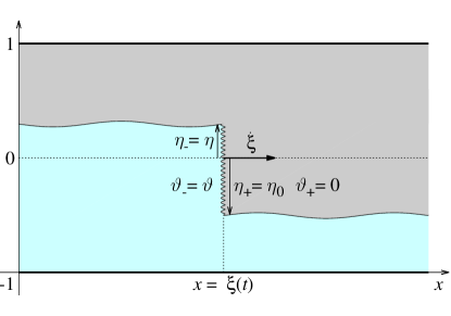
Figure 2: A jump with the upstream interface height $\eta_{-}=\eta$ and the shear velocity $\vartheta_{-}=\vartheta$ propagating at the speed $\dot{\xi}$ into a still fluid ahead $(\vartheta_{+}=0)$ with the interface located at the height $\eta_{+}=\eta_{0}.$

Consider a hydraulic jump which occurs over a length scale comparable to the layer depth and thus appears in the SW approximation as a discontinuity in $\eta$ and $\vartheta$ at the point $x=\xi(t)$ across which the respective variables jump by $\left\llbracket\eta\right\rrbracket\equiv\eta_{+}-\eta_{-}$ and $\left\llbracket\vartheta\right\rrbracket\equiv\vartheta_{+}-\vartheta_{-}.$ Here the plus and minus subscripts denote the corresponding quantities at the front and behind of the jump. The double-square brackets stand for the differential of the enclosed quantity across the jump. Integrating Eqs. (25) and (26) across the jump, which is equivalent to substituting spatial derivative $f_{x}$ with $\left\llbracket f\right\rrbracket$ and time derivative $f_{t}$ with $-\dot{\xi}\left\llbracket f\right\rrbracket$ [51], the jump propagation velocity can be expressed, respectively, as

$$\dot{\xi} = \frac{1}{2}\frac{\left\llbracket\vartheta(1-\eta^{2})\right\rrbracket}{\left\llbracket\eta\right\rrbracket},$$ (29)

$$\dot{\xi} = \frac{1}{4}\frac{\left\llbracket\eta^{2}+\vartheta^{2}-3\eta^{2}\vartheta^{2}+2\alpha\eta(1-\vartheta^{2})\right\rrbracket}{\left\llbracket(\alpha+\eta)\vartheta\right\rrbracket}.$$ (30)

As for single layer, the jump conditions consist of two equations and contain five unknowns: $\eta_{\pm},$ $\vartheta_{\pm}$ and $\dot{\xi}.$ Consequently, two unknown parameters can be determined when the other three are specified. Since the jump conditions are non-linear, multiple solutions are possible. Some of these solutions may be unphysical. Feasible solutions are selected by an additional constraint which follows from the energy equation (23). Integrating this equation as described above, we obtain the following difference of energy fluxes across the jump

$$\left\llbracket\eta\vartheta(1-\eta^{2})(1-\vartheta^{2})-\dot{\xi}\left(\eta^{2}+\vartheta^{2}-\eta^{2}\vartheta^{2}\right)\right\rrbracket=\dot{\varepsilon}\leq 0.$$ (31)

This quantity cannot be positive because there is no physical mechanism which could generate energy in the jump. Energy can be either dissipated or dispersed by the short non-hydrostatic waves excited by the jump [3].

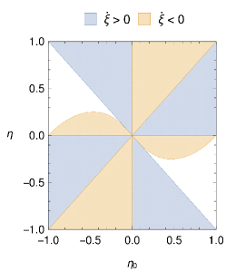
Figure 3: The downstream $(\eta_{0})$ and upstream $(\eta)$ heights of bores permitted by the hyperbolicity constraint $\vartheta^{2}\leq 1$ for $\alpha=0$ (a), $\infty$ (b), $-1$ (c), $1$ (d). The downstream $(\dot{\xi}>0)$ and upstream $(\dot{\xi}<0)$ directions of propagation are defined by the energy constraint $\dot{\varepsilon}\leq 0.$

Next, let us apply general jump conditions (29,30) to a bore with the upstream interface height $\eta_{-}=\eta$ which propagates into a quiescent fluid $(\vartheta_{+}=0)$ with the interface located at the height $\eta_{+}=\eta_{0},$ as shown in Fig. 2. After a few rearrangements, the upstream shear velocity $\vartheta_{-}=\vartheta$ and the propagation speed can expressed, respectively, as

$$\vartheta^{\pm} =\pm\frac{(\eta_{0}-\eta)(\eta_{0}+\eta+2\alpha)^{1/2}}{((1-\eta^{2})(\eta_{0}-\eta)+2(\eta+\alpha)(1-\eta_{0}\eta))^{1/2}},$$ (32)

$$\dot{\xi}^{\pm} =-\vartheta^{\pm}\frac{1-\eta^{2}}{2(\eta_{0}-\eta)},$$ (33)

where the plus and minus signs refer to the opposite directions of propagation, i.e., $\dot{\xi}^{+}=-\dot{\xi}^{-},$ which are both permitted by the mass and momentum balance conditions. Because the energy balance (31) changes sign with the direction of propagation, only one direction is usually permitted for the bore of given height. The possible downstream $(\eta_{0})$ and upstream $(\eta)$ heights of bores permitted by the hyperbolicity constraint $(\vartheta^{2}\leq 1)$ and their direction of propagation are shown in Fig. 3 for various $\alpha.$ As discussed before, $\alpha=0$ corresponds to the basic momentum equation (22), in which both layers contribute equally to the pressure drop across the jump. $\alpha=1$ and $\alpha=-1$ correspond to the pressure drops determined by the top and bottom layer, respectively. $\alpha\rightarrow\infty$ corresponds to the circulation conservation law (24), which is based on the assumption that the pressure drops across the discontinuity in both layers are equal. The downstream and upstream heights which satisfy the hyperbolicity constraint depend on $\alpha$. For each such combination of heights, bore can propagate either downstream $(\dot{\xi}>0)$ or upstream $(\dot{\xi}<0)$ depending on the energy constraint (31). As seen in Fig. 3, the respective regions in the $(\eta_{0},\eta)$ plane for $\alpha=0$ and $\alpha=\infty$ are centrally symmetric, whereas for $\alpha=\pm 1$ they are centrally reflected images of each other. The last two values exclude the bores with $\eta_{0}\rightarrow\pm 1,$ which correspond to deep and shallow downstream states, respectively.

In all four cases, the direction of propagation can be seen in Fig. 3 to reverse along two lines: $\eta=\eta_{0}$ and $\eta=0.$ The first (diagonal) line corresponds to infinitesimal-amplitude waves. In this limit, the propagation speed (33) becomes equal to the characteristic velocity (28). The second (horizontal middle) line corresponds to the bores with the upstream interface located at the channel mid-height. These bores are exceptional. First, in contrast to all other bores, they conserve the energy and, thus, can propagate in either direction. Second, their velocity of propagation is independent of their height and equal to $\pm\frac{1}{2}$ for all $\alpha$. It means that these bores conserve also the circulation. These are exactly the properties of the so-called solibores (see Eqs. (3.33) and (3.34) in [19]) which appear as permanent-shape solutions in the weakly non-hydrostatic approximation described by Eq. (11).

Gravity currents correspond to the limiting case of bores which propagate along the bottom $(\eta_{0}=-1).$ As seen in Fig. 3, the depth of gravity currents is limited to the channel mid-height $(\eta\leq 0)$ for all considered values of $\alpha$ except $\alpha=1.$ For a gravity current which propagates downstream, Eqs. (32) and (33) yield

$$\vartheta = \left(\frac{(1+\eta)(1-\eta-2\alpha)}{1-\eta^{2}-2(\alpha+\eta)}\right)^{1/2},$$ (34)

$$\dot{\xi} = \frac{1}{2}(1-\eta)\vartheta.$$ (35)

The propagation velocity (35) can be written in terms of the traditional front height $h=(1+\eta)/2$ as

$$\dot{\xi}=(1-h)\sqrt{\frac{2h(1-\alpha-h)}{1-\alpha-2h^{2}}}.$$ (36)

As seen in Fig. 4 for $\alpha=0,$ this SW front velocity is generally slightly lower than that resulting from the well-known Benjamin’s formula $\dot{\xi}=\sqrt{\frac{h(1-h)(2-h)}{1+h}}$ [8], whereas the vortex-sheet model of Borden and Meiburg [11] yields a somewhat higher front velocity $\dot{\xi}=(1-h)\sqrt{2h}.$ It is noteworthy that the same propagation velocity results also from the SW circulation conservation equation (24) which corresponds to $|\alpha|\rightarrow\infty$ in Eq. (36).

It turns out that also Benjamin’s formula follows from Eq. (36) with $\alpha=-1,$ which corresponds to the pressure along the interface determined solely by the bottom layer. In the control-volume approach, this is interpreted as the conservation of energy in the bottom layer. Such an interpretation is based on the assumption that the flow in the hydraulic jump is stationary. As argued above in relation to Eq. (19), such an assumption is not compatible with the hydrostatic SW approximation. It is also interesting to note that Eq. (36) reproduces the general vortex-sheet formula derived by Ungarish and Hogg [50] when the ratio of the so-called head losses in the top and bottom layer is substituted with $\frac{\alpha+1}{\alpha-1}.$ Implications of this rather non-obvious mathematical equivalence will be discussed in the conclusion.

We include in Fig. 4 also the recent results of Ungarish and Hogg [50] for gravity currents obtained using the vortex-wake model in which a shear layer of finite-thickness is assumed instead of sharp interface. The assumption of a diffuse interface takes this model outside the scope of the SW approximation. All models can be seen to yield the same velocity for thin layers $(h\rightarrow 0):$ $\dot{\xi}/\sqrt{h}\rightarrow\sqrt{2},$ which is the classical result due to von Kármán [25], as well as for the gravity currents spanning the lower half of the channel $(h=1/2):$ $\dot{\xi}/\sqrt{h}=1/\sqrt{2}.$ For intermediate heights, the SW model with $\alpha=0$ produces generally lower front velocities than the previous models.

Based on the experimental observations, it has been suggested by Rottman and Simpson [44] and Marino et al. [35] that for shallow gravity currents, the normalized front velocity $\dot{\xi}/\sqrt{h}$ may be closer to $1$ rather than $\sqrt{2}.$ Numerical results indicate that this discrepancy may be due to turbulent interfacial drag [30] or viscosity [23]. The latter can have a significant effect even on relatively deep gravity currents up to Reynolds numbers of $O(10^{4})$, which are typical for laboratory experiments. Alternatively, it may be due to the uncertainty in the depth of turbulent gravity currents. As shown in the next section, shallow gravity currents can be connected to a range of deeper upstream states. Taking the upstream depth as the front height results in a lower-than-expected normalized front velocity.

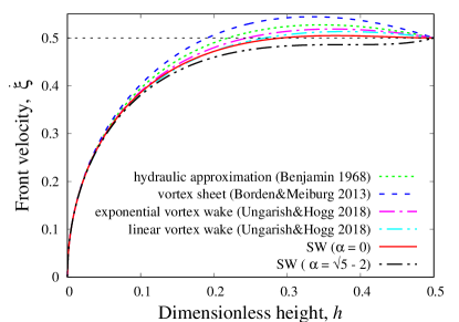
Figure 4: The front velocity of gravity current $\dot{\xi}$ versus the dimensionless front height $h=\frac{1}{2}(1+\eta):$ comparison of the SW result for $\alpha=0$ and $\alpha=\sqrt{5}-2$ with the classical hydraulic approximation due to Benjamin [8], the vortex sheet model of Borden and Meiburg [11] and the vortex-wake model of Ungarish and Hogg [50].

Klemp et al. [30] argue that causality does not permit gravity current to move faster than the characteristic wave velocity (28)

$$\lambda^{+}=-\eta\vartheta+\frac{1}{2}\sqrt{(1-\eta^{2})(1-\vartheta^{2})}.$$

If so, the gravity current height $h=(1+\eta)/2$ cannot exceed

$$h_{c}=\begin{cases}(\sqrt{3}-1)/2,&\alpha=0,\\ 2\sin(\pi/18),&\alpha=-1,\\ 1/3,&\alpha\rightarrow\infty,\end{cases}$$ (37)

where the last last two values correspond to the front conditions of Benjamin [8] and Borden and Meiburg [11]. It has to be noted, however, that the front moving at a supercritical speed (faster than the disturbances behind it) does not violate causality as long as there are faster moving disturbance ahead of it. This is indeed the case for the disturbances at the bottom of gravity current (see Fig. 5a).

There are two more noteworthy coincidences which occur at the critical height. First, as seen in the inset of Fig. 5, the point at which the characteristic velocity $\left.\lambda_{+}\right|_{z=h}$ drops below the front speed $\dot{\xi}$ for the corresponding height at given $\alpha$ coincides with the maximum of $\dot{\xi}.$ Baines [6] following Benjamin [8] argue that the presence of such a maximum implies that gravity currents with $h>h_{c}$ are unstable and, thus, physically impossible. Namely, if $h\geq h_{c}$ and correspondingly $\frac{d\dot{\xi}}{dh}<0,$ then a virtual perturbation that reduces the front height $h$ would increase the front speed $\dot{\xi.}$ By the mass conservation, this would further reduce the front height thus enhancing the initial perturbation. As a result, the gravity current would collapse to a stable subcritical height $h\leq h_{c}.$ This is a physical mechanism which can limit the height of gravity current to the critical value (37). Alternatively, by the same arguments, the instability can result in the increase of the front height up the channel mid-height. According to Fig. 3, this is the maximal height gravity current can have for all considered values of $\alpha$ except $\alpha=1.$

The second coincidence, pointed out already by Benjamin [8], concerns the energy dissipation rate which also attains a maximum at exactly the same critical height. The underlying mechanism and consequences of these two non-obvious coincidences will be elucidated in the next section, where we consider the possible upstream states to which gravity current can be connected via an intermediate bore.

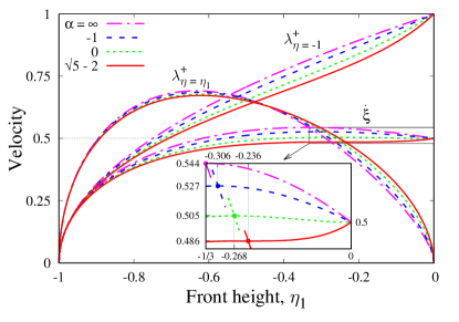
Figure 5: The characteristic downstream wave speed $\lambda^{+}$ at the top $(z=h)$ and bottom $(z=0)$ of the front and the front velocity $\dot{\xi}$ versus its height for $\alpha=\infty,-1,0,\sqrt{5}-2$ (a) and the corresponding energy dissipation (b).

It has to be noted that the coincidence of the maximal front propagation velocity with the characteristic wave speed pointed out above is limited to

$$\alpha<\alpha_{c}=\sqrt{5}-2\approx 0.236.$$ (38)

The same applies also to the occurrence of maximal dissipation rate at the critical height. For $\alpha>\alpha_{c},$ the intersection point of the propagation and characteristic velocities switches over to the minimum of $\dot{\xi}$ which emerges at $\eta=-\alpha<0$ and moves towards the maximum as $\alpha$ rises above zero. At $\alpha=\alpha_{c},$ the minimum and maximum of $\dot{\xi}$ merge forming a stationary inflection point at the critical interface height $\eta_{c}=-\alpha_{c},$ where $\partial_{\eta}\dot{\xi}=\partial_{\eta}^{2}\dot{\xi}=0.$ The front height and the propagation speed at this point are $h_{c}=(1-\alpha_{c})/2\approx 0.382$ and $\dot{\xi_{c}}=\alpha_{c}^{1/2}\approx 0.486$ (see Fig. 5). At $\alpha>\alpha_{c},$ the inflection point vanishes as two local extrema of $\dot{\xi}$ re-emerge. At $\alpha=\frac{1}{2},$ the minimum of $\dot{\xi}$ moves back to $h=\frac{1}{2}.$ At this point, the maximum of energy dissipation rate switches from the maximum to minimum of $\dot{\xi}.$

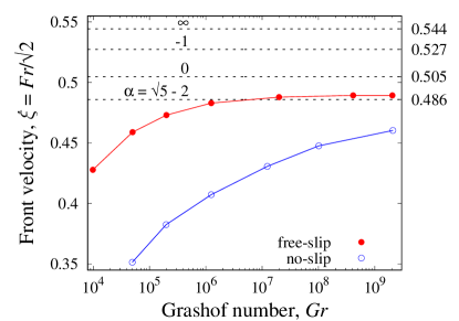
Figure 6: Comparison of critical gravity current speeds for various $\alpha$ with the numerical results of Härtel et al. [23] for gravity currents generated by the lock exchange with free-slip and no-slip boundary conditions. The conversion factor of $1/\sqrt{2}$ is due to the channel half-height used as the length scale in the definition of Froude number $\mathit{Fr}$ by Härtel et al. [23]; Grashof number defines the magnitude of the driving force and thus the characteristic flow velocity with the Reynolds number $\mathit{Re}\sim\sqrt{\mathit{Gr}}.$

Thus, $\alpha_{c}$ represents an exceptional point at which the gravity current speed becomes a monotonically increasing function of its depth. It is interesting to note that the propagation velocity at this point agrees surprisingly well with the highly-accurate numerical results of Härtel et al. [23] for the gravity currents generated by the full lock exchange with free-slip boundary conditions (see Fig. 6). With real no-slip boundary conditions, a much higher Reynolds number seems to be required to attain this inviscid limit. As shown below, $\alpha_{c}$ produces a remarkably good agreement with numerical results not only for gravity currents but also for a wide range of bores in Boussinesq fluids.

Let us now turn to bores and compare their propagation velocities resulting from the SW theory with the predictions of some previous models as well as with the available experimental and numerical data. For comparison, we choose the semi-empirical model of Klemp, Rotunno and Skamarock (KRS) [31], the vortex-sheet model of Borden and Meiburg (BM) [11] and the vortex-wake model of Ungarish and Hogg (UH) [50]. The KRS model is known to achieve a better agreement with the experimental results by assuming that energy is dissipated only in the top layer, which shrinks as the bore advances. The BM model is based on the 2D vorticity equation which is applied in the integral form to bores in Boussinesq fluids. As for the gravity currents, the BM model yields exactly the same front speed as the SW circulation conservation law (24): $\dot{\xi}=\frac{1}{2}(1-\eta^{2})/(1-\eta_{0}\eta)^{1/2}.$ In the UH model, the conservation of both the circulation and momentum is effectively imposed in addition to that of the mass. This is not possible using only the height averaged quantities in each layer, as in the SW approximation, and requires a non-uniform vertical velocity distribution. The latter is introduced by replacing the sharp interface with a single-parameter shear layer. The form of this layer is not uniquely defined and affects the results as it may be seen in Fig. 4.

The aforementioned models are compared in Fig. 7 with the experimental results of Wood and Simpson [53], Rottman and Simpson [44] and Baines [4] as well as with the two-dimensional numerical results of Borden et al. [12]. Note that the ratio of densities $s=\rho^{-}/\rho^{+}=0.79$ used by Baines [4] is somewhat lower than $s=1$ assumed in the Boussinesq approximation. Nevertheless, there is no noticeable deviation of the experimental results from the Boussinesq approximation when the average density is used as the characteristic value. For consistency with previous studies, all front velocities are rescaled with $\sqrt{h_{0}},$ which is the dimensionless velocity of small-amplitude long interfacial waves when the depth of the bottom layer ahead of the bore is small $(h_{0}\ll 1).$ The front velocities normalized in this way are plotted in Fig. 7 against the bore strength $h/h_{0},$ where $h$ is the upstream interface height. With this normalization, we have $\dot{\xi}/\sqrt{h_{0}}\rightarrow 1$ when the downstream layer is thin $(h_{0}\rightarrow 0)$ and the bore is weak $(h/h_{0}\rightarrow 1).$ All models can be seen to converge to this essentially linear limit. Although the predicted front velocities start to diverge at larger bore strengths, the divergence remains small relative to the scatter in the experimental data. All front velocities converge again, as for the gravity current velocity in Fig. 4, when the interface height approaches the mid-plane $h=0.5.$ The same front velocity produced by all models implies that all underlying conservation laws are satisfied simultaneously in this particular case. As noted before, this is the case for all bores with the upstream interface located at the channel mid-height.

The SW front velocity (33) for $\alpha=0$ is seen to approach this limit tangentially. This is due to the distinctive feature of this model, which yields $\frac{\mathrm{d}\dot{\xi}}{\mathrm{d}h}=0$ at $h=0.5,$ whereas all other models have $\frac{\mathrm{d}\dot{\xi}}{\mathrm{d}h}<0$ at this point. Numerical results for $h_{0}=0.2$ can be seen in Fig. 7(d) to reproduce this nearly monotonous variation predicted by the SW model with $\alpha=0$, though at sightly lower propagation velocities. This difference, which is usually attributed to the turbulent mixing between the layers, may also be due to viscous loss of momentum at the rigid top and bottom boundaries. Viscous effects are assumed to be negligible in the SW model but could be significant at the relatively small Reynolds number $\mathit{Re}=3500$ used in the numerical simulation by Borden et al. [12].

A remarkably better agreement with numerical results is produced by the SW model with $\alpha=\alpha_{c}=\sqrt{5}-2.$ As discussed above Eq. (38), physical considerations suggest that gravity currents exceeding a certain critical height, which depends on $\alpha$ and is defined by the maximal propagation velocity for that $\alpha$, are unstable. The largest height a stable gravity current can have is attained at $\alpha=\alpha_{c}.$ This maximization of the front height may be a dynamical mechanism behind the selection of $\alpha_{c}.$

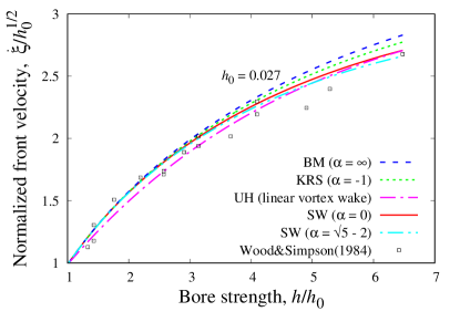
Figure 7: The front velocity $\dot{\xi}/\sqrt{h_{0}}$ normalized with the dimensionless depth of the bottom layer $h_{0}$ ahead the bore versus the bore strength $h/h_{0}$ for $h_{0}=0.027,0.035,0.05,0.1,0.2:$ comparison of the SW theory $(\text{SW, }\alpha=0,\sqrt{5}-2$) with KRS [31], BM [11], UH [50] models as well as with the experimental results of Wood and Simpson [53], Rottman and Simpson [44], Baines [4] and the numerical results of Borden et al. [12].

4 Bores trailing gravity currents

In the previous section, we showed that bores which propagate into the quiescent downstream state can be described using the SW jump conditions (29,30). These conditions can be applied also to more complex jump configurations as it is demonstrated in this section for bores which can form on the top of gravity currents. The presence of such bores can make the front of gravity current shallower than the far upstream state. This may explain why experimentally observed propagation velocities of shallow gravity currents are lower than the theoretical predictions based on the upstream height.

Now, instead of the quiescent fluid layer shown in Fig. 2, the downstream state is assumed to be a gravity current with the interface height $\eta_{0}$ and the shear velocity $\vartheta_{+}=\vartheta_{0}(\eta_{0})$ which is defined by Eq. (34) with $\eta_{0}$ substituted for $\eta$. As before, the upstream height $\eta_{-}=\eta_{1}$ and the associated shear velocity $\vartheta_{-}=\vartheta_{1}$ need to be found by solving Eqs. (29, 30). For $\alpha=0,$ using the computer algebra software Mathematica [52], we obtain:

$$\vartheta_{1}^{\pm}(\eta_{1},\eta_{0})=\frac{(\eta_{1}+\eta_{0})(1-\eta_{1}\eta_{0})\vartheta_{0}\pm(\eta_{1}-\eta_{0})\gamma}{\eta_{1}+\eta_{0}-3\eta_{1}^{2}\eta_{0}+\eta_{1}^{3}},$$ (39)

where $\gamma^{2}=\eta^{2}\left(\left(4\eta_{1}^{2}-1\right)\vartheta_{0}^{2}-3\eta_{1}^{2}+1\right)-2\eta_{0}\eta_{1}\left(\eta_{0}^{2}+\vartheta_{0}^{2}-1\right)+\eta_{1}^{2}\left(\eta_{1}^{2}-\vartheta_{0}^{2}+1\right)$ and the plus and minus signs denote two possible branches of the solution. A similar but somewhat longer solution can be obtained also for general $\alpha.$ For $\eta_{1}=\eta,$ Eq. (39) reduces to $\vartheta_{1}^{\pm}=\vartheta_{0},$ which corresponds to a uniform gravity current of the height $\eta_{0}.$

Let us first consider a shallow gravity current of the depth $h_{0}=(1+\eta_{0})/2\rightarrow 0$ and assume the upstream state to be of a comparably small depth:

$$h_{1}=(1+\eta_{1})/2=\kappa h_{0},$$ (40)

where $\kappa=h_{1}/h_{0}=O(1).$ In this limit, the propagation velocity (33) for the shear velocity $\vartheta$ defined by Eq. (39) becomes independent of $\alpha:$

$$\dot{\xi}_{1}=\left(1\mp\frac{\kappa}{\sqrt{\kappa+1}}\right)\dot{\xi}_{0},$$ (41)

where $\dot{\xi}_{0}=\sqrt{2h_{0}}$ is the velocity of gravity current for $h_{0}\rightarrow 0.$ As seen, only the velocity defined by the minus sign is physically feasible, i.e., $\dot{\xi}_{1}\leq\dot{\xi}_{0}.$ Note that the bore velocity drops with the increase of its relative height $\kappa$ and turns zero at

$$\kappa_{0}=\left(1+\sqrt{5}\right)/2.$$

At this height ratio, the bore turns into a stationary hydraulic jump. On the other hand, the energy balance defined by Eq. (31), which reduces to

$$\dot{\varepsilon}_{1}=\frac{4\sqrt{2}(\kappa-1)^{3}\left(\kappa-\sqrt{\kappa+1}\right)}{(\kappa+1)^{3/2}}h_{0}^{5/2},$$ (42)

indicates that the bore satisfies the energy constraint $\dot{\varepsilon}_{1}\leq 0$ only for $1\leq\kappa\leq\kappa_{0}.$ It means that a shallow gravity current can be connected to an upstream state which is up to a factor of $\kappa_{0}$ taller. Taking the maximum possible upstream depth as the effective gravity current height reduces the normalized front speed from $\sqrt{2}$ to $\dot{\xi}/\sqrt{h_{1}}=2/\sqrt{1+\sqrt{5}}\approx 1.11.$ It is interesting to note that for a fixed upstream height $(\kappa h_{0}=\text{const}),$ $\dot{\varepsilon}_{1}$ defined by Eq. (42) attains minimum at $\kappa_{c}\approx 1.414.$ This yields the normalized front speed $\dot{\xi}/\sqrt{h_{1}}\approx 1.189,$ which is very close to the empirical value of $1.19$ found for $h_{1}<0.075$ by Huppert and Simpson [26].

The exact solution of Eq. (31) plotted in Fig. 8 shows that the possible upstream depth for deeper gravity currents is larger than that predicted by the linear relationship (40) for shallow currents. Nevertheless, the height of maximal energy loss for a fixed upstream depth remains relatively close to this line also for deeper currents.

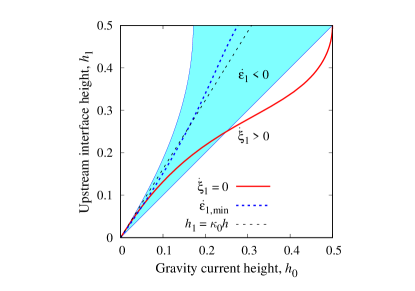
Figure 8: The upstream interface height $h_{1}$ permitted by the energy balance constraint $\dot{\varepsilon}_{1}\leq 0$ defined by Eq. (31) versus the gravity current height $h_{0}$ for the positive (a) and the negative (b) branches of Eq. (39) $(\alpha=0).$ The dotted lines show the upper limit for shallow gravity currents $(h_{1}=\kappa_{0}h_{0})$ and the depth at which the energy loss attains maximum ($\dot{\varepsilon}_{1,\min})$; the solid lines show the interface height at which the upstream jump becomes stationary $(\dot{\xi}_{1}=0)$ (a) and moving at the same speed as the gravity current $\dot{(\xi}_{1}=\dot{\xi}_{0})$ (b).

First, let us consider the possibility of a shallower gravity current forming at the front of a supercritical current with $h\geq h_{c}.$ This corresponds to a relatively deep leading gravity current connected to a taller upstream state via single bore which moves in the same direction as the gravity current. As seen in Fig. 8(a), if the leading gravity current is sufficiently shallow, the bores described by the positive branch of Eq. (39) can move downstream only. The bores that can trail deep gravity currents are described by the negative branch of Eq. (39). The corresponding height of gravity current and that of bore, which are admitted by the energy balance constraint (31), are shown by the filled-in region on Fig. 8(b). The solid line delimits the range of bores whose speed of propagation does not exceed that of the leading gravity current. The interface heights that satisfy both constraints are located in the upper right corner below the diagonal line $(h_{1}\leq h_{0})$ on Fig. 8(b). This corresponds to an upstream state which is shallower than the leading gravity current head. The latter, in turn, has to be taller than the minimal depth defined by the intersection of the diagonal with the solid line along which $\dot{\xi}_{1}=\dot{\xi}_{0}.$ This point coincides with the critical depth $h_{c}$ at which the leading front speed attains maximum and becomes unstable at $h>h_{c}.$

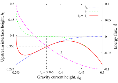
Figure 9: The bore height $h_{1}$ versus the depth of gravity current $h_{0}$ at which both move at the same speed $\dot{\xi}_{1}=\dot{\xi}_{0}$ along with the energy balance defined by Eq. (31) for the gravity current $(\dot{\varepsilon}_{0})$ and the bore $(\dot{\varepsilon}_{1})$.

It may also be seen in Fig. 8(b) that stable gravity currents, which are located in the region above the diagonal with $h_{0}<h_{c}<h_{1},$ give rise only to energy-generating bores. The latter are unphysical when considered as separate entities. Hypothetically, such bores can exist together with a leading gravity current provided that no total energy is generated by the system of the two coupled jumps. However, for such a coupled system to form, the bore has to move at the same speed as the leading front, i.e., $\dot{\xi}_{1}=\dot{\xi}_{0}$. The jump heights which satisfy this constraint are shown by the solid line in 8(b). As seen in Fig. 9, although the bore generates energy if $h_{0}<h_{c},$ more energy is dissipated by the leading gravity current front as long as the upstream state is shallower than the channel mid-height $h_{1}=0.5$. This critical upstream depth produces a leading gravity current of the lowest possible depth $h_{0}=1-1/\sqrt{2}\approx 0.293$ for $\alpha=0.$ The corresponding depths for $\alpha=-1$ and $\alpha=\infty$ are $(5-\sqrt{17})/4\approx 0.219$ and $(3-\sqrt{5})/4\approx 0.191,$ respectively. The decrease of the upstream depth causes the leading gravity current depth rise until both become equal at $h_{c}$ which is defined by Eq. (37). At this point, the bore height becomes small relative to the underlying gravity current. Thus, its velocity of propagation approaches that of small-amplitude disturbances. This velocity equals the characteristic wave speed $\lambda_{+}$ defined by Eq. (28). It explains why $\lambda_{+}$ coincides with the maximum of $\dot{\xi}$ exactly rather than just approximately as speculated by Baines [6]. It also reveals the duality of the propagation velocity for gravity currents of a supercritical depth $h_{1}\geq h_{c}.$ Firstly, $\dot{\xi}=\dot{\xi}(h_{1})$ defines the velocity of a gravity current of depth $h_{1}.$ Secondly, this velocity is equal to the velocity of a bore with the same upstream height which trails the gravity current of a subcritical depth $h_{0}<h_{c}$ propagating at the same speed $\dot{\xi}=\dot{\xi}(h_{0})$.

5 Summary and Conclusion

In this paper, we derived a locally conservative SW momentum equation for the two-layer system bounded by a rigid lid. The equation contains a free dimensionless parameter $\alpha,$ which defines the relative contribution of each layer to the pressure gradient along the interface. This equation can describe strong internal bores and gravity currents in a self-contained way without invoking external front conditions. So far such closure conditions were presumed to be indispensable and derived using various control-volume methods. The momentum equation (18) was obtained for two fluids with arbitrary density difference by using a linear combination of the basic SW equations (9), which describe the conservation of irrotationality in each layer, to eliminate the pressure gradient along the interface. Applying the Boussinesq approximation to fluids with a small density difference, the momentum equation reduced to Eq. (21). Finally, using the velocity and height differentials as dynamical variables, this equation was written in the dimensionless form as Eq. (26).

The appearance of the free parameter $\alpha$ in the general form of the momentum equation is closely related with the presence of the external length scale, the total height $H,$ in the considered two-layer system. Namely, using the fact that the circulation conservation equation (12) is a one-order-lower SW conservation law in terms of the height than the momentum equation (17), we can multiply the former with a coefficient $\propto H$ and then add it to the latter. Such an operation is formally permitted because both equations have the same physical units. This leads to the generalized momentum conservation equation containing $\alpha$ and the associated component of the circulation conservation law. The $\alpha$-term in the generalized momentum equation (18) vanishes if this equation is satisfied simultaneously with the circulation conservation equation (12). This, however, is the case for smooth waves but not in general for hydraulic jumps.

Dimensional as well as physical considerations suggest that if $\alpha$ is constant, as it is required by the equivalence of momentum and circulation conservation laws for smooth waves, it can depend only on the ratio of densities, which is the sole dimensionless parameter in this problem. As the dynamical pressure produced by the flow is proportional to the density of fluid, for nearly equal densities, both layers can be expected to affect the interfacial pressure gradient with approximately equal weight coefficients. This corresponds to $\alpha\approx 0.$

The jump propagation velocity (33) which results from the Rankine-Hugoniot jump conditions (29, 30) for the mass conservation equation (25) and the momentum equation (26) with $\alpha=0$ was compared with the predictions of a number of previous models as well as with the numerical and experimental results. A good agreement was found with the available data including those for moderately non-Boussinesq fluids. The propagation velocities resulting from the SW model with $\alpha=0$ appear generally closer to the numerical results than the those predicted by the previous models. We note that a mathematically equivalent result is produced by the so-called vortex-sheet model of Ungarish and Hogg [50] using the head loss ratio $\lambda=-1.$ However, negative head loss ratios are not compatible with the basic control volume assumptions. This is discussed in more detail below as well as in the Appendix.

A particularly good agreement with high-accuracy numerical results for both gravity currents and bores is produced by $\alpha_{c}=\sqrt{5}-2.$ At this exceptional value, the gravity current speed becomes a monotonically increasing function of its depth. At all other $\alpha,$ the gravity current speed attains a maximum at certain critical depth which depends on $\alpha.$ Simple physical considerations suggest that gravity currents of supercritical depth are unstable. The largest front height that a stable gravity current can have is attained at $\alpha_{c}$. We hypothesize that this value may be selected dynamically when an unstable gravity current collapses from a supercritical height to the largest possible stable height. Alternatively, the instability may cause the front height to increase producing an elevated gravity current head which may rise up to the channel mid-height as it is shown by the exact analytical solution as well as observed in 2D numerical simulation of the partial lock exchange problem [43, 29].

We also showed that the classical front condition for gravity currents obtained by Benjamin [8] as well as its generalization to internal bores by Klemp et al. [(KRS) 31] are reproduced by the SW momentum equation with $\alpha=-1.$ This value describes the interfacial pressure gradient which is determined entirely by the bottom layer. Similarly, the alternative front condition proposed earlier by Wood and Simpson [53], which is known to yield a generally poorer agreement with experimental results than the KRS model and to break down for shallow gravity currents, is reproduced by the SW model with $\alpha=1.$ This value describes the interfacial pressure gradient determined solely by the top layer.

According to the traditional interpretation, in the WS model, the energy is conserved in the top layer and lost only in the bottom layer, while in the KRS model, it is the other way round Li and Cummins [32]. argue that, in general, energy can be lost simultaneously in both layers. If so, then the WS and KRS models would represent two limiting cases and yield, respectively, the upper and lower bound on the bore velocity. It is important to note that the bore velocities resulting from the SW model with $\alpha=0$ are lower than those predicted not only by the WS but also by the KRS model. This is because only the total energy for both layers together is defined in the SW framework. It is important stress that this is a rigorous mathematical fact rather than a deficiency of the SW model, in which one layer can gain energy from the other as long as the total energy does not increase across the jump. The latter condition, which is defined by Eq. (31), determines in which direction bore can propagate. In the conventional control-volume approach, the energy exchange between the layers is absent because the interface is assumed to be stationary in the co-moving frame of reference. Therefore, in a self-consistent control-volume approach, neither layer can gain energy and hence neither head loss can be negative [32].

There is no such a constraint in the SW framework, where the pressure drop across the hydraulic jump in each layer follows from the conservation of irrotationality (9). If the interface in the hydraulic jump is stationary in the co-moving frame of reference, as it is commonly assumed in the control-volume approach, the same pressure drop would result also from the energy conservation in each layer which is described by Eq. (19). Such an assumption, however, is unphysical and leads to a paradox which is illustrated below by the circulation conservation condition. It is important to note that, in the hydrostatic SW approximation, the solution that is stationary (in the co-moving frame of reference) cannot be continuous (and the other way round) [51]. The control-volume analysis being an integral approach misses this essential mathematical subtlety.

The circulation conservation condition is effectively based on the assumption that the pressure drop across the jump is the same in both layers. In the control-volume approach, the corresponding pressure drops are assumed to follow from the conservation of energy in each layer. The paradox is that the assumed conservation of energy across the jump in each layer separately does not guarantee the conservation of energy in both layers together. It is because, in the hydrostatic SW approximation as well as in the control-volume approach, the energy across the jump cannot in general be conserved simultaneously with the mass and circulation. This paradox appears also in the inviscid limit of the vortex-sheet model of [50] who attribute it to the inadequacy of the inviscid approximation. From the SW perspective described above, this paradox is due to the inadequacy of the energy conservation assumption in separate fluid layers.

Similar to the energy also the circulation cannot in general be conserved simultaneously with the momentum and mass. In the SW framework, this is known as the Rankine-Hugoniot deficit [27]. The conservation of a given quantity depends on the physical mechanisms which are outside the scope of the SW approximation but could become relevant in the hydraulic jumps. Such mechanisms are, for example, the viscous dissipation and turbulence, which can account for the loss of energy and the generation of circulation in strong bores. But there is no analogous physical mechanism which could disrupt the momentum balance in highly inertial flows. Therefore, the momentum conservation, notwithstanding its inherent ambiguity, appears physically more relevant than the conservation of circulation and energy.

The main advancement of the proposed theory is the realization that internal bores and gravity currents can be described using hydrostatic SW approximation which was previously thought impossible. The proposed SW theory provides not only a mathematically consistent and rational alternative to the conventional control-volume approach but also a self-contained framework for numerical modeling of strong internal bores and gravity currents in the two-layer systems bounded by a rigid lid. A canonical example is the lock-exchange problem which can be solved analytically by the method of characteristics and used as a benchmark to validate numerical solution of the locally conservative SW water equations derived in this study [43].

Appendix

This section presents an extended discussion of the key differences between the proposed SW theory and two alternative approaches [11, 50]. The first is that of Borden and Meiburg [11] who argue that since the vorticity front condition can be decoupled from the pressure drop, the latter can be determined, if required, independently from the former by substituting the jump parameters that satisfy this front condition into the momentum balance condition. So both conditions would be satisfied simultaneously along with the conservation of mass. This, however, is at odds not only with the SW theory but also with the inviscid limit of the vortex-sheet model of Ungarish and Hogg [50] which is physically equivalent to the model of Borden and Meiburg [11]. The fact that the vorticity equation, which Borden and Meiburg [11] integrate over the control volume enclosing the jump, contains no pressure, does not decouple the latter from the vorticity front condition. It is important to note that the 2D integral of the vorticity transport equation considered by Borden and Meiburg [11] is mathematically equivalent by Stokes’ theorem to the circulation of Euler equation along the boundary of the control volume [50]. Therefore, it is not mathematically consistent to accept one approach and dismiss the other as done, for example, by Khodkar et al. [29] with respect to Bernoulli’s law which underlies the vorticity front condition. The pressure drop across a circulation-conserving hydraulic jump is indeed defined by the second approach. This pressure drop, however, is not necessarily the same as that satisfying the momentum balance condition. Thus, the latter cannot be satisfied together with the circulation conservation unless the model is substantially extended by introducing two additional phenomenological parameters, the so-called head losses, which are supposed to account for the effect of viscous dissipation on the pressure drop [50].

Borden and Meiburg [11] also argue that their vorticity front condition must satisfy the momentum balance because so does the vorticity equation it is derived from. The SW equations, which follow from the mathematically equivalent Euler equation, demonstrate that the equivalence of the associated conservation laws relies on the continuity of the velocity and pressure fields. Continuity is required only by the PDEs, which describe local conservation laws, but not by the integral conservation laws, which are actually employed for the derivation of approximate front conditions using the control-volume method.

The second alternative approach is the vortex-sheet model of Ungarish and Hogg [50]. As noted before, the front speed resulting from the Rankine-Hugoniot jump conditions of the generalized SW momentum and mass conservation equations is mathematically equivalent to that resulting from the vortex-sheet model when the ratio of head losses is expressed as $\lambda=\frac{\alpha-1}{\alpha+1}.$ This equivalence is intriguing because the head loss is a phenomenological quantity which is introduced in the control-volume approach to account for the viscous energy losses in each layer. Such a quantity, however, is completely outside the scope of the SW theory, which neither requires nor allows energy dissipation to be attributed to a particular layer. In contrast to the head loss, the free parameter $\alpha$ which features in the SW theory is not a phenomenological parameter modeling something outside the SW approximation. As a matter of fact, $\alpha$ is an intrinsic parameter of the two-layer SW system bounded by rigid lid where it emerges due to the inherent non-uniqueness of the SW momentum equation.

It has be noted that Ungarish and Hogg [50] substantially extend the original meaning of head loss by associating it with the viscous flux of vorticity through the adjacent horizontal boundary. The inferred direction of this flux is then used to conclude that head loss must be positive in the top layer and negative in the bottom layer. This may be in agreement with numerical simulations but, as noted in the conclusion, it is not consistent with the stationarity of the interface, which is assumed in the control-volume approach and requires the head losses in both layers to be non-negative [32].

There are two more questionable assumptions underlying the vortex-sheet model. First, Ungarish and Hogg [50] consider a viscous fluid but substitute the physical no-slip conditions at the solid top and bottom walls with artificial free-slip conditions. This substitution is essential for the control-volume method to be applicable. On the other hand, the exact boundary conditions at the top and bottom walls may not be that relevant as indicated by the numerical simulations 23.

However, the main premise of the vortex-sheet model is that the balance of vorticity, which is generated by the the baroclinic torque at the interface and then advected by the flow along the layer, can significantly be affected by the viscous vorticity fluxes through the top and bottom boundaries at which a zero vorticity is imposed by the free-slip boundary conditions. There are two problems with this assumption in relation to highly inertial flows which are typical for turbulent internal bores and gravity currents. Firstly, at high Reynolds numbers, the vorticity generated by the baroclinic torque at the interface is predominantly advected downstream, especially in the upper layer. Thus, the vorticity remains confined within a relatively thin layer forming along the interface, as it is assumed in the more refined vortex-wake model [50]. As a result, the vorticity is advected out of the control volume through the downstream side boundary well before it reaches the top wall. Besides that the free-slip boundary condition allows the flow along the top wall to remain irrotational far downstream from the control volume. Consequently, there can be no significant viscous flux of vorticity through the upper boundary of the control volume. This is confirmed by the numerical results of Nasr-Azadani and Meiburg [39], who find no significant difference between the free-slip (zero vorticity) and zero-vorticity-flux boundary conditions.

The same argument as above holds also for the bottom layer except the gravity currents for which this layer is nearly quiescent in the co-moving frame of reference. Although the viscous vorticity flux can be relatively significant in this case, one needs to take into account the characteristic vorticity diffusion time $\sim H^{2}/\nu$ which is necessary for a steady vorticity flux to develop. This time is $\sim\mathit{Re}\gtrsim 10^{4}$ relative to the time $\sim H/U$ taken by fluid to flow over a horizontal distance comparable to the layer depth. It means that viscous vorticity fluxes cannot develop on the time scale relevant to the propagation of turbulent internal bores and gravity currents. In addition, it should be noted that there is no viscous dissipation along at the boundaries when free-slip is assumed. This makes the association of head losses with viscous vorticity fluxes problematic.

In addition, the fact that only the ratio of head losses appears in the general vortex-sheet front condition implies that these two phenomenological quantities are not mutually independent. Firstly, they are related to each other through the pressure balance condition at the interface. This condition is equivalent to the pressure compatibility condition used by Ungarish and Hogg [50]. Secondly, in the hydrostatic approximation, the head losses along the top and bottom boundaries follow directly from the pressure drop along the interface. The latter is the key quantity in the SW model where it is defined using single parameter $\alpha$ while the head losses may be regarded as secondary quantities depending on $\alpha$.

References

- Abbott [1961] M. B. Abbott. On the spreading of one fluid over another. La Houille Blanche, 6:827–856, 1961.
- Abgrall and Karni [2009] R. Abgrall and S. Karni. Two-layer shallow water system: a relaxation approach. SIAM J. Sci. Comput., 31(3):1603–1627, 2009.
- Ali and Kalisch [2010] A. Ali and H. Kalisch. Energy balance for undular bores. C.R. Mec., 338(2):67–70, 2010.
- Baines [1984] P. G. Baines. A unified description of two-layer flow over topography. J Fluid Mech, 146:127–167, 1984.
- Baines [1995] P. G. Baines. Topographic effects in stratified flows. Cambridge University Press, 1995.
- Baines [2016] P. G. Baines. Internal hydraulic jumps in two-layer systems. J. Fluid Mech., 787:1–15, 2016.
- Barros [2006] R. Barros. Conservation laws for one-dimensional shallow water models for one and two-layer flows. Math. Models Methods Appl. Sci., 16(01):119–137, 2006.
- Benjamin [1968] T. B. Benjamin. Gravity currents and related phenomena. J. Fluid Mech., 31(2):209–248, 1968.
- Benjamin [1984] T. B. Benjamin. Impulse, flow force and variational principles. IMA J. Appl. Math., 32(1-3):3–68, 1984.
- Benjamin [1986] T. B. Benjamin. On the boussinesq model for two-dimensional wave motions in heterogeneous fluids. J. Fluid Mech., 165:445–474, 1986.
- Borden and Meiburg [2013] Z. Borden and E. Meiburg. Circulation-based models for Boussinesq internal bores. J. Fluid Mech., 726:R1, 2013.
- Borden et al. [2012] Z. Borden, E. Meiburg, and G. Constantinescu. Internal bores: an improved model via a detailed analysis of the energy budget. J. Fluid Mech., 703:279–314, 2012.
- Camassa et al. [2012] R. Camassa, S. Chen, G. Falqui, G. Ortenzi, and M. Pedroni. An inertia ’paradox’ for incompressible stratified euler fluids. J Fluid Mech, 695:330–340, 2012.
- Cavanie [1969] A. G. Cavanie. Sur la genese et la propagation d’ondes internes dans un millieu a deux couches. Cahiers Océanographiques, XXI(9):831–843, 1969.
- Choi and Camassa [1999] W. Choi and R. Camassa. Fully nonlinear internal waves in a two-fluid system. J. Fluid Mech., 396:1–36, 1999.
- Christie and White [1992] D. R. Christie and R. White. The morning glory of the gulf of carpentaria. Aust. Meteorol. Mag, 41:21–60, 1992.
- Chumakova et al. [2009] L. Chumakova, F. E. Menzaque, P. A. Milewski, R. R. Rosales, E. G. Tabak, and C. V. Turner. Stability properties and nonlinear mappings of two and three-layer stratified flows. Stud. Appl. Math., 122(2):123–137, 2009.
- Courant and Friedrichs [1948] R. Courant and K. O. Friedrichs. Supersonic flow and shock waves. Interscience, New York, 1948.
- Esler and Pearce [2011] J. G. Esler and J. D. Pearce. Dispersive dam-break and lock-exchange flows in a two-layer fluid. J. Fluid Mech., 667:555–585, 2011.
- Evans and Ziegler [2007] J. W. Evans and D. P. Ziegler. The electrolytic production of aluminumn. In A. J. Bard, editor, Encyclopedia of Electrochemistry. Wiley, 2007. ISBN 9783527610426.
- Fyhn et al. [2019] E. H. Fyhn, K. Y. Lervåg, Å. Ervik, and Ø. Wilhelmsen. A consistent reduction of the two-layer shallow-water equations to an accurate one-layer spreading model. Phys. Fluids, 31(12):122103, 2019. URL https://doi.org/10.1063/1.5126168.
- Green and Naghdi [1976] A. E. Green and P. M. Naghdi. Directed fluid sheets. Proc. R. Soc. Lond. A, 347(1651):447–473, 1976.
- Härtel et al. [2000] C. Härtel, E. Meiburg, and F. Necker. Analysis and direct numerical simulation of the flow at a gravity-current head. part 1. flow topology and front speed for slip and no-slip boundaries. J. Fluid Mech., 418:189–212, 2000.
- Helfrich and Melville [2006] K. R. Helfrich and W. K. Melville. Long nonlinear internal waves. Annu. Rev. Fluid Mech., 38:395–425, 2006.
- Huppert [2006] H. E. Huppert. Gravity currents: a personal perspective. J. Fluid Mech., 554:299–322, 2006.
- Huppert and Simpson [1980] H. E. Huppert and J. E. Simpson. The slumping of gravity currents. J. Fluid Mech., 99(4):785–799, 1980.
- Kalisch et al. [2017] H. Kalisch, D. Mitrovic, and V. Teyekpiti. Delta shock waves in shallow water flow. Phys. Lett. A, 381(13):1138–1144, 2017.
- Kelley and Weier [2018] D. H. Kelley and T. Weier. Fluid mechanics of liquid metal batteries. Appl. Mech. Rev., 70(2):020801, 2018.
- Khodkar et al. [2017] M. A. Khodkar, M. M. Nasr-Azadani, and E. Meiburg. Partial-depth lock-release flows. Phys. Rev. Fluids, 2(6):064802, 2017.
- Klemp et al. [1994] J. B. Klemp, R. Rotunno, and W. C. Skamarock. On the dynamics of gravity currents in a channel. J. Fluid Mech., 269:169–198, 1994.
- Klemp et al. [1997] J. B. Klemp, R. Rotunno, and W. C. Skamarock. On the propagation of internal bores. J. Fluid Mech., 331:81–106, 1997.
- Li and Cummins [1998] M. Li and P. F. Cummins. A note on hydraulic theory of internal bores. Dyn Atmos Oceans, 28(1):1–7, 1998.
- Liska et al. [1995] R. Liska, L. Margolin, and B. Wendroff. Nonhydrostatic two-layer models of incompressible flow. Computers Math. Applic., 29(9):25–37, 1995.
- Long [1956] R. R. Long. Long waves in a two-fluid system. J. Meteor., 13(1):70–74, 1956.
- Marino et al. [2005] B. M. Marino, L. P. Thomas, and P. F. Linden. The front condition for gravity currents. J. Fluid Mech., 536:49–78, 2005.
- Milewski et al. [2004] P. Milewski, E. Tabak, C. Turner, R. Rosales, and F. Menzaque. Nonlinear stability of two-layer flows. Comm. Math. Sci., 2(3):427–442, 2004.
- Milewski and Tabak [2015] P. A. Milewski and E. G. Tabak. Conservation law modelling of entrainment in layered hydrostatic flows. J. Fluid Mech., 772:272–294, 2015.
- Montgomery and Moodie [2001] P. J. Montgomery and T. B. Moodie. On the number of conserved quantities for the two-layer shallow-water equations. Stud. Appl. Math., 106(2):229–259, 2001.
- Nasr-Azadani and Meiburg [2015] M.M. Nasr-Azadani and E. Meiburg. Gravity currents propagating into shear. J. Fluid Mech., 778:552–585, 2015.
- Ostapenko [1999] V. V. Ostapenko. Complete systems of conservation laws for two-layer shallow water models. J. Appl. Mech. Tech. Phys., 40(5):796–804, 1999.
- Ovsyannikov [1979] L. V. Ovsyannikov. Two-layer "shallow water" model. J. Appl. Mech. Tech. Phys., 20(2):127–135, 1979.
- Pedlosky [1979] J. Pedlosky. Geophysical fluid dynamics. Springer, 1979.
- Politis and Priede [2022] G. Politis and J. Priede. Lock-exchange problem for Boussinesq fluids revisited: exact shallow-water solution. Phys. Fluids, 34:106602, 2022.
- Rottman and Simpson [1983] J. W Rottman and J. E. Simpson. Gravity currents produced by instantaneous releases of a heavy fluid in a rectangular channel. J. Fluid Mech., 135:95–110, 1983.
- Rotunno et al. [2011] R. Rotunno, J. B. Klemp, G. H. Bryan, and D. J. Muraki. Models of non-Boussinesq lock-exchange flow. J. Fluid Mech., 675:1–26, 2011.
- Sandstrom and Quon [1993] H. Sandstrom and C. Quon. On time-dependent, two-layer flow over topography. i. hydrostatic approximation. Fluid Dyn. Res., 11(3):119, 1993.
- Scotti and Pineda [2004] A. Scotti and J. Pineda. Observation of very large and steep internal waves of elevation near the massachusetts coast. Geophys. Res. Lett., 31(22), 2004.
- Stoker [1958] J. J. Stoker. Water waves: The mathematical theory with applications. Wiley, 1958.
- Ungarish [2011] M. Ungarish. Two-layer shallow-water dam-break solutions for non-Boussinesq gravity currents in a wide range of fractional depth. J. Fluid Mech., 675:27–59, 2011.
- Ungarish and Hogg [2018] M. Ungarish and A. J. Hogg. Models of internal jumps and the fronts of gravity currents: unifying two-layer theories and deriving new results. J. Fluid Mech., 846:654–685, 2018.
- Whitham [1974] G. B. Whitham. Linear and Nonlinear Waves. Wiley, 1974.
- Wolfram [2003] S. Wolfram. The Mathematica Book. Wolfram Media, 2003.
- Wood and Simpson [1984] I. R. F. Wood and J. E. Simpson. Jumps in layered miscible fluids. J. Fluid Mech., 140:329–342, 1984.
- Yih and Guha [1955] C.-S. Yih and C. R. Guha. Hydraulic jump in a fluid system of two layers. Tellus, 7(3):358–366, 1955.