$(K,L)$-eigenvectors in max-min algebra

Abstract

Using the concept of $(K,L)$-eigenvector, we investigate the structure of the max-min eigenspace associated with a given eigenvalue of a matrix in the max-min algebra (also known as fuzzy algebra). In our approach, the max-min eigenspace is split into several regions according to the order relations between the eigenvalue and the components of $x$. The resulting theory of $(K,L)$-eigenvectors, being based on the fundamental results of Gondran and Minoux, allows to describe the whole max-min eigenspace explicitly and in more detail.

1 Introduction

By max-min algebra we mean the unit interval $\mathbb{B}=<0,1>$ equipped with the arithmetic operations of ”addition” $a\oplus b=\max(a,b)$ and ”multiplication” $a\otimes b=\min(a,b)$. Algebraically speaking, max-min algebra is a semiring where both arithmetic operations are idempotent. Let us also note that, algebraically, max-min algebra is an example of incline algebra of [4].

The arithmetic operations $\oplus$ and $\otimes$ can be extended to matrices and vectors in the usual way so that for any matrices $A=(a_{ij})$ and $B=(b_{ij})$ of appropriate dimensions we can define their ”sum” $A\oplus B$ and ”product” $A\otimes B$ by the usual rules: $(A\oplus B)_{ij}=a_{ij}\oplus b_{ij}$ and $(A\otimes B)_{ij}=\bigoplus_{k}a_{ik}\otimes b_{kj}$. For a square matrix $A\in\mathbb{B}^{n\times n}$ we can also define its max-min matrix powers: $A^{k}=\underbrace{A\otimes\ldots\otimes A}_{k}$, where $k$ is a natural number. Note that $A^{0}=I$, the usual identity matrix. Further we will systematically omit the product sign $\otimes$, for brevity.

As usual in tropical/idempotent algebras, to each matrix $A\in\mathbb{B}^{n\times n}$ we associate a digraph ${\mathcal{D}}(A)=(N,E)$ with the node set $N=\{1,\ldots,n\}$ and edge set $E=\{(i,j)\colon a_{ij}>0\}$. Each edge has a weight $a_{ij}$. A sequence of edges $(i_{0},i_{1}),(i_{1},i_{2}),\ldots,(i_{k-1},i_{k})$ where each edge belongs to $E$ is called a walk whose length is $k$ and whose weight is given by the max-min product $a_{i_{0}i_{1}}\dots a_{i_{k-1}i_{k}}$.

One of the motivations to study max-min algebra comes from the theory of fuzzy sets where the operation $\min(a,b)$ is one of the most useful examples of triangular norms, see Klement, Mesiar and Pap [19]. See also Gondran and Minoux [17] for more on semirings and other algebraic models relevant to the theory of fuzzy sets.

The main goal of the present paper is to further investigate the structure of the max-min eigenspace associated with a given eigenvalue. For a given matrix $A\in\mathbb{B}^{n\times n}$ and a number $\lambda\in\mathbb{B}$, the max-min eigenspace associated with $\lambda$ is the set of vectors $x\in\mathbb{B}^{n\times 1}$ (called $\lambda$-eigenvectors) such that

$$Ax=\lambda x.$$ (1)

Note that it is indeed a space in the sense of max-min algebra: for any $\alpha,\beta\in\mathbb{B}$ and any $u$ and $v$ satisfying (1) $\alpha u\oplus\beta v$ also satisfies this equation. Let us now give some examples to motivate the study of this eigenproblem and our approach to it.

Example 1.1 (Medical symptoms and therapy)

One of the first models, in which the max-min eigenvectors were used, was concerned with searching invariants in therapeutic recommendations. It was put forward by Sanchez [27], see also a monograph by Rakus-Andersson [26] for a more recent account of this method and more references. In this model, the matrix $A\in\mathbb{B}^{n\times n}$ expresses a fuzzy relation describing the relative success of treating $n$ symptoms of some illness by some drug. In this matrix, a diagonal entry $a_{ii}$ is equal to the recovery rate from the $i$th symptom, and entry $a_{ij}$, for any $i\neq j$ is, the rate at which either both symptoms $i$ and $j$ are absent after the application of drug, or symptom $i$ is absent and symptom $j$ is still present. In other words, $a_{ij}$ is the rate at which “the action of the drug is equal or stronger on the $i$th symptom than on the $j$th symptom” [26], designed to account for the link between the symptoms and action of the drug on them. The max-min eigenvectors $x$ associated with eigenvalue $1$ appear as eigen fuzzy sets. Note that in this application, one is usually interested in the greatest left eigenvector of $A$, i.e., the greatest $x$ such that $xA=x$. This vector, together with some other vector, is then used to estimate reliable intervals for the rate at which a drug removes the $n$ symptoms.

The greatest max-min eigenvector is easy to use, as it can be quickly found by a simple iterative procedure [28, 26]. However, it can be seen as giving an overly optimistic judgement, and in this situation one may be interested 1) to impose a condition that the recovery rate is no bigger than $\lambda$ and 2) to require that certain components of vector $x$, while being below $\lambda$, stay at their initial level $x_{i}$. A further development of this idea in the context of medical treatments is beyond the scope of the present paper.

The greatest left max-min eigenvectors of a given matrix $A$ with entries in the interval $[0,1]$ were also used by Nobuhara et al. [25] in image reconstruction, where a given image was encoded by means of max-min and min-max eigenvectors of $A$, as well as fixed points of various convex combinations of the max-min and min-max products associated with $A$, and then successfully reconstructed using them.

Example 1.2 (Security in a computer framework)

This example was put forward as a motivation for studying strongly tolerant interval eigenvectors in max-min algebra [13]. A computer network consisting of servers $S_{1},\ldots,S_{n}$, data storage units $D_{1},\ldots,D_{n}$ and a logical unit $L$ is considered. Lines $K_{ij}$, for $i,j\in I$, connect $S_{i}$ with $D_{j}$, while lines $L_{j}$ connect every $D_{j}$ with $L$. The security level of each line in the network is measured by values in the real interval $[0,1]$, where value $0$ stands for completely unsecure connection and value $1$ stands for completely secure connection. The security of every $K_{ij}$ (data security) is denoted by $a_{ij}$, and the security of $L_{j}$ (logic security) is denoted by $x_{j}$. The maximal security level $y_{i}$ of information transfer from servers $S_{i}$ to the logical unit $L$ through the given storage units is the $i$th component of the vector $y=A\otimes x$. If we wish to keep the data security unchanged by the information transfer from servers $S_{i}$ to the logical unit $L$ through the given storage units, then $y=x$ should hold. Moreover, we have to consider the security level of the system itself, which depends on the accessible technologies and the available budget. The technological security of the system can decrease the security of the processed data below the level $\lambda$, for some $\lambda\in\langle 0,1\rangle$, and then $\lambda x$ becomes new target level of security. Note that $A(\lambda x)=\lambda x$ in max-min algebra, which means that the invariance of the new levels of security will be ensured. If we additionally require that the new levels of security should become exactly equal to $\lambda$ in some components and stay equal to $x_{i}$ in the others, then we are led to study $(K,L)$- eigenvectors, introduced and studied in the present paper.

Problem (1) has been studied in max-min algebra at least since Gondran and Minoux [15, 16] and Sanchez [27]. The approach taken in [15, 16] resembles that of max-plus algebra, where eigenspaces are characterized as particular subspaces of the column span of Kleene star. There is also a number of works where a different approach is taken. Sanchez [27, 28] is focused on the largest eigenvector associated with the eigenvalue $1$ and suggests an algorithm that can be used to compute it in practice. In the same vein, Cechlárová [6] describes lower and upper basic eigenvectors in terms of the associated graph. The structure of the eigenspace of increasing max-min eigenvectors $x_{1}\leq x_{2}\leq\ldots\leq x_{n}$ in max-min algebra is described by Gavalec [10], and various types of max-min interval eigenvectors have been studied in Gavalec et al. [14].

Gondran and Minoux obtained fundamental results for (1) also over more general semirings with idempotent multiplication, see [18][Section 6.3] for one of the latest accounts. We are going to use these results. However, we observe that the theory as presented in that monograph describes only the solutions whose all components are less than or equal to $\lambda$ [18][Ch. 6, Corollary 3.5]. Several examples when (1) also admits other solutions can be found in the present paper. To describe those other solutions we adopt an approach which is similar to that of Gavalec et al. [12], where the eigenproblem in max-Łukasiewicz algebra was studied (see also Gavalec and Němcová [11]). Namely, given $A$ and $\lambda$ we consider a partition of $N=\{1,\ldots,n\}$ into two disjoint subsets $K$ and $L$ such that $K\cup L=N$ and pose a problem of describing all $\lambda$-eigenvectors $x$ that satisfy $x_{i}\leq\lambda$ and hence $\lambda x_{i}=x_{i}$ for all $i\in K$ and $x_{i}\geq\lambda$ and hence $\lambda x_{i}=\lambda$ for all $i\in L$. When $K=N$ we call such vectors ”principal $\lambda-$eigenvectors” since (1) becomes $Ax=x$, and when $L=N$ we call such vectors ”background $\lambda$-eigenvectors”, in analogy with [12]. In the latter case (1) becomes $Ax=\lambda\mathbf{1}$, where $\mathbf{1}$ denotes the vector of all $1$’s. principal eigenvectors were described in [18][Ch. 6, Corollary 3.5], which we revisit here in Corollary 3.2. Background eigenvectors are easy to obtain: see Proposition 3.1 and Proposition 3.2 below. Principal and background $\lambda$-eigenvectors are fundamental for describing the $(K,L)-$eigenvectors associated with $\lambda$ in the case of general $K$, $L$ and $\lambda$. Their description is stated in Theorem 3.1, which can be considered as our main result.

Theorem 3.1 also yields a method for constructing a generating set for the whole $\lambda$-eigenspace, although the computational effort may grow exponentially with matrix size. First of all, note that, for general $K$ and $L$, the set of $(K,L)-$eigenvectors is not a max-min space any more, since the set $\{x\colon x_{i}\geq\lambda\}$ is not a max-min space. However, it is a max-min convex set: if $x$ and $y$ are $(K,L)$-eigenvectors associated with $\lambda$ and $\alpha\oplus\beta=1,$ then $\alpha x\oplus\beta y$ is also such a $(K,L)$-eigenvector. This follows since (like in the usual convexity) any max-min space is a max-min convex set, and the sets defined by max-min affine inequalities such as $x_{i}\leq\lambda$ or $x_{i}\geq\lambda$ are also max-min convex. For arbitrary vectors $x^{1},\ldots,x^{n}\in\mathbb{B}^{n}$ one can consider their max-min convex combinations: $\alpha_{1}x^{1}\oplus\ldots\oplus\alpha_{n}x^{n}$ where $\alpha_{1}\oplus\ldots\oplus\alpha_{n}=1$ is required, and the set of all such combinations (for given $x^{1},\ldots,x^{n}$) is called the max-min convex hull of these points. Some max-min convex sets are max-min convex hulls of a finite number of points. The easiest and most important example is $\mathbb{B}^{n}$, which is the max-min convex hull of the zero vector $\mathbf{0}$ and unit vectors $e^{i}$, whose $i$the component is equal to $1$ and the rest of the components are equal to $0$. Theorem 3.1 will provide for a comprehensive description of any set of $(K,L)$-eigenvectors as a max-min convex hull of a finite number of points. Then we can take the union of these sets and obtain a set of points whose max-min convex hull is the whole $\lambda$-eigenspace. Taking out the zero vector $\mathbf{0}$, we then obtain a generating set for the whole $\lambda$-eigenspace. See, e.g., Nitica and Sergeev [23, 24] for more on max-min convexity.

All new results of this paper are obtained in Section 3. Preliminary notions and results from Gondran and Minoux [18] and Butkovič et al. [3], which provide the necessary algebraic tools, are given in Section 2.

2 Some problems of max-min algebra

In this section we will give some necessary notions and facts from max-min algebra on which our study of max-min $(K,L)$-eigenvectors will be based. We will start with defining the notions of metric matrix and Kleene star and (following Gondran and Minoux [18]) giving a description of the set of principal eigenvectors ($x$ such that $Ax=x$). This will be followed by describing the solution set to max-min Bellman ($Z$-matrix) equation (following Butkovič et al. [3] or Krivulin [21]) and solving a special type of max-min equation (8) in Subsection 2.2.

2.1 Metric matrix, Kleene star and the principal eigenproblem

For a square matrix $A\in\mathbb{B}^{n\times n}$ let us define its metric matrix $A^{+}=(a^{+}_{ij})_{i,j=1}^{n}$ and Kleene star $(a^{*}_{ij})_{i,j=1}^{n}$ by the following series:

$$\begin{split}A^{+}&=A\oplus A^{2}\oplus A^{3}\oplus\ldots\\ A^{*}&=I\oplus A\oplus A^{2}\oplus\ldots\end{split}$$ (2)

where $I$ denotes the identity matrix, whose diagonal entries are equal to $1$ and off-diagonal entries are $0$. It is well-known that in max-min algebra these series always converge and, moreover, can be truncated:

$$\begin{split}A^{+}&=A\oplus\ldots\oplus A^{n},\\ A^{*}&=I\oplus A\oplus\ldots\oplus A^{n-1}.\end{split}$$ (3)

In terms of the associated graph, $a^{+}_{ij}$, being equal to $a^{*}_{ij}$ when $i\neq j$, is the maximal (max-min) weight of all walks connecting $i$ to $j$ with unrestricted length. So is the optimal walk interpretation of metric matrices and Kleene stars.

Metric matrices, Kleene stars and associated digraphs provide some of the basic tools for the max-min eigenproblem. Let us start with the principal eigenproblem: the problem of identifying all vectors $x$ that satisfy $Ax=x$ for a given matrix $A$. Such vectors are called principal eigenvectors of $A$.

For each principal eigenvector $x$, following the terminology of [1], define its saturation graph $\operatorname{Sat}(A,x)$ as the graph consisting of all edges $(i,j)$ that satisfy $a_{ij}\otimes x_{j}=x_{i}$ and all nodes on these edges. This graph in general has several maximal strongly connected components, and let $C(A,x)$ denote a subset of $N=\{1,\ldots,n\}$ that contains one node from each strongly connected component of $\operatorname{Sat}(A,x)$. We now state a description of the set of principal eigenvectors, which is due to [18].

Theorem 2.1 (Gondran-Minoux [18] Section 6.3)

The set of principal eigenvectors is a max-min space generated by vectors

$$a_{ii}^{+}(A^{*})_{\cdot i},\quad i=1,\ldots,n.$$ (4)

More precisely, each vector of (4) is a principal eigenvector, and each principal eigenvector $x$ can be represented as

$$x=\bigoplus_{i\in C(A,x)}x_{i}a_{ii}^{+}(A^{*})_{\cdot i}.$$ (5)

We will also use the theory of algebraic Bellman equation

$$x=Ax\oplus b,$$ (6)

studied over general semirings, e.g., in Carré [5], Litvinov and Maslov [22]. In nonnegative linear algebra this equation is also known as $Z$-matrix equation [3].

Although (6) has been known for decades, the following fundamental result, describing the whole solution set to (6), was formulated only recently in Butkovič et al. and Krivulin [3, 20, 21].

Theorem 2.2

Let $A\in\mathbb{B}^{n\times n}$ and $b\in\mathbb{B}^{n}$. Equation (6) always has solutions, and the set of these solutions is

$$\{A^{*}b\oplus v\colon Av=v\}.$$ (7)

2.2 Special type of equation

We also need to describe the solution set for the system

$$Az\oplus b=\lambda\mathbf{1}.$$ (8)

where $A\in\mathbb{B}^{m\times n}$, $z\in\mathbb{B}^{n}$ and $b\in\mathbb{B}^{m}$ (for arbitrary natural numbers $m$ and $n$).

We will study this system under the condition that all coefficients of $A$ and $b$ are less than or equal to $\lambda$:

$$a_{ij}\leq\lambda,\quad b_{i}\leq\lambda\quad\forall i,j\in N.$$ (9)

The description will be obtained in terms of coverings and minimal coverings, following the known solution method for systems of the form $A\otimes x=b$ and $A\otimes x\geq b$ in max-plus and max-min algebra (see, e.g., Butkovič [2], Cunninghame-Green and Cechlárová [8], and Elbassioni [9]).

Note that if the system (8) is solvable, then in every row of the equation, we have to obtain $\lambda$ either from $Az$ or from $b$.

Let us denote $I_{0}=\{i\colon b_{i}<\lambda\}$ and $C_{j}=\{i\in I_{0}\colon a_{ij}=\lambda\}$ for $j\in N$.
Furthermore, for $W\subseteq N$ we denote $C^{W}$ and $z^{W}$ by putting

$$C^{W} =\bigl{\{}C_{j}\colon j\in W\bigr{\}}$$ (10)

$$z^{W}_{j} =\left\{\begin{array}[]{ll}\lambda&\text{if }\ j\in W\\ 0&\text{otherwise}\end{array}\right.$$ (13)

We say that $C^{W}$ is a covering of $I_{0}$, if $I_{0}=\bigcup C^{W}(=\bigcup_{j\in W}C_{j})$. Moreover, $C^{W}$ is a minimal covering of $I_{0}$, if

$$I_{0}\neq\bigcup C^{V}\,\text{ for every }\,V\subseteq W,\,V\neq W.$$ (14)

Proposition 2.1

$z\in\mathbb{B}^{n}$ is a solution of (8) with condition (9) if and only if $z\geq z^{W}$ for some $W\subseteq N$ such that $C^{W}$ is a minimal covering of $I_{0}$.

Proof: Suppose $z\in\mathbb{B}^{n}$ is a solution of (8). Then $b_{i}<\lambda$ implies $(A_{i})z=\lambda$. Then, also using (9), we obtain that for every $i\in I_{0}$ there is $j=j(i)\in N$ with $a_{ij(i)}=\lambda$ and $z_{j(i)}\geq\lambda$. Denoting $W=\{j(i)\colon i\in I_{0}\}$ , we get $I_{0}=\bigcup C^{W}$ and $z\geq z^{W}$. Without loss of generality, we can assume that the covering $C^{W}$ of $I_{0}$ is a minimal one.

For the converse implication, suppose $z\geq z^{W}$ for some $W\subseteq N$, with $C^{W}$ being a minimal covering of $I_{0}$. Then, for any $i\in I_{0}$, there is $j=j(i)\in W$ such that $i\in C_{j(i)}$. That is, $z_{j(i)}\geq z^{W}_{j(i)}=\lambda$ and $a_{ij(i)}=\lambda$, which gives $(A_{i})z=\lambda$.  $\square$

Corollary 2.1

Equation (8) with condition (9) is solvable if and only if there exists a covering $C^{W}$ of $I_{0}$. In this case, solution set to (8) can be represented as $\bigcup_{W}S^{W}$ where the union is taken over $W\subseteq N$ such that $C^{W}$ is a minimal covering of $I_{0}$ and

$$\begin{split}S^{W}:&=\{z\colon z^{W}\leq z\leq\mathbf{1}\}\\ &=\{z\colon\lambda\leq z_{k}\leq 1\ \text{for $k\in W$},\ z_{k}\geq 0\ \text{for $k\in N\setminus W$}\},\end{split}$$ (15)

Note that if $I_{0}=\emptyset$ then the minimal covering of $I_{0}$ is $C^{W}$ with $W=\emptyset$ and the unique minimal (and hence the least) solution of (8) is $\mathbf{0}$ and the solution set is $\{z\colon\mathbf{0}\leq z\leq\mathbf{1}\}$.

Set $S^{W}=\{z\colon z^{W}\leq z\leq\mathbf{1}\}$ can be also algebraically expressed as follows.

$$S^{W}=\{z^{W}\oplus v_{N}\colon v_{N}\in\mathbb{B}^{|N|}\}$$ (16)

Example 2.1

We shall illustrate the solution of (8) by the following system:

$$A=\begin{pmatrix}.3&.5&.3\\ .6&.6&.2\\ .6&.3&.6\end{pmatrix},\ b=\begin{pmatrix}.6\\ .3\\ .2\end{pmatrix}$$

and consider $\lambda=.6$.

Then the set $I_{0}=\{2,3\}$. From the entries of $A$ we can derive sets $C_{1}=\{2,3\},C_{2}=\{2\}$ and $C_{3}=\{3\}$.

For $W=\{1\}$, we have $C^{W}=\{C_{1}\}$. This set is a minimal covering of $I_{0}$, the minimal solution here is $z^{W}=z^{\{1\}}=(.6,0,0)$ and every $z\geq z^{\{1\}}$ is also a solution, i.e. $S^{\{1\}}=\{z^{\{1\}}\oplus v\colon v\in\mathbb{B}^{3}\}$.

Similarly, for $W=\{2,3\}$ we have the set $C^{W}=\{C_{2},C_{3}\}$ which is minimal covering of $I_{0}$ with minimal solution $z^{W}=z^{\{2,3\}}=(0,.6,.6)$. Again, also vectors $z\geq z^{\{2,3\}}$ are solutions to the system, i.e. $S^{\{2,3\}}=\{z^{\{2,3\}}\oplus v\colon v\in\mathbb{B}^{3}\}$

Final solution set for the system (8) is then represented by the union of particular solution sets, $\bigcup_{W}S^{W}$.

3 Max-min eigenproblem

Let us first consider some two-dimensional examples that show how the solution to the max-min eigenproblem (1) splits into subsets of $(K,L)$-eigenvectors.

Example 3.1

Take

$$A=\begin{pmatrix}.7&.3\\ .2&.5\end{pmatrix}$$ (17)

and consider $\lambda=.5$. Then the solution of (1) is equivalent to the system

$$\max\bigl{(}\min(.7,x_{1}),\min(.3,x_{2})\bigr{)}=\min(.5,x_{1}),$$ (18)

$$\max\bigl{(}\min(.2,x_{1}),\min(.5,x_{2})\bigr{)}=\min(.5,x_{2})$$ (19)

The solution set for (18) is

$$X^{\prime}=\Bigl{\{}(x_{1},x_{2})\colon((x_{1}\geq.3)\vee(x_{1}\geq x_{2}))\wedge(x_{1}\leq.5)\Bigr{\}},$$ (20)

and the solution set for 19 is

$$X^{\prime\prime}=\Bigl{\{}(x_{1},x_{2})\colon(x_{2}\geq.2)\vee(x_{1}\leq x_{2})\}\Bigr{\}}.$$ (21)

Then, the solution set to the eigenproblem is $X^{\prime}\bigcap X^{\prime\prime}$. Sets $X^{\prime}$, $X^{\prime\prime}$ and their intersection are displayed in Figure 1.

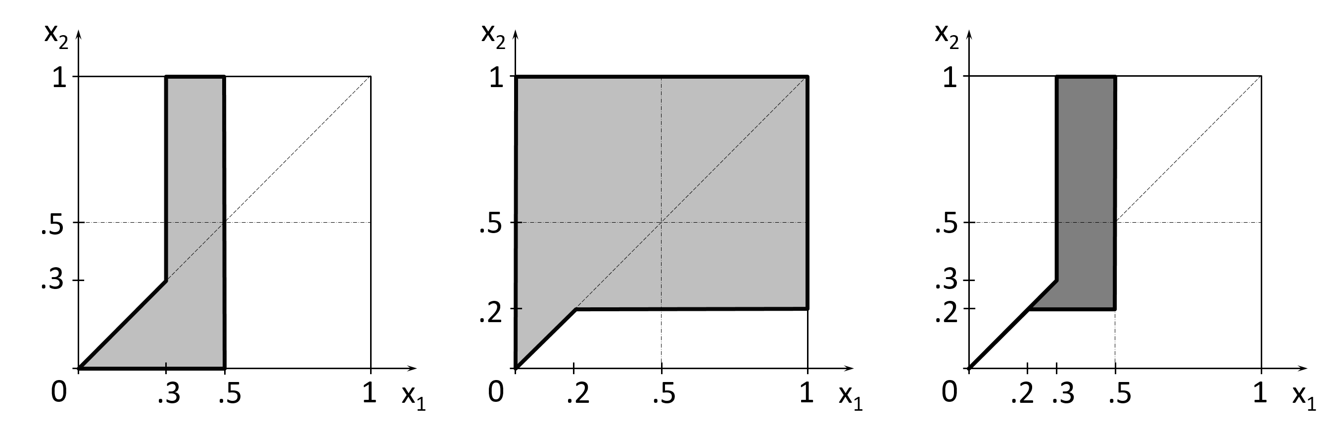
Figure 1: Sets $X^{\prime}$, $X^{\prime\prime}$ and their intersection: the $0.5$-eigenspace of $A$

In Figure 2 we observe the effect of the value $\lambda$ on the final solution set. The eigenvectors can be thus studied in individual areas (subsets) defined by $\lambda$. The boundaries of these areas represented by the dashed line divide the solution set of our two-dimensional example into four areas (in figure quadrants $Q_{1}-Q_{4}$).

For the eigenvectors in $Q_{1}$ it holds that all $x_{i}\geq\lambda$ and thus we say that all $i\in L$ and $K=\emptyset$. We call these eigenvectors the background eigenvectors of $A$. For $Q_{2}$ and $Q_{3}$ it holds that $x_{i}\leq\lambda$ for some $i\in K$ and some $x_{i}\geq\lambda$ for some $i\in L$. In $Q_{4}$ all $x_{i}\leq\lambda$, it means that all $i\in K$ and $L=\emptyset$. We call these vectors the principal eigenvectors of $A$.

Note that in example 3.1 we have some “genuine” $(K,L)$-eigenvectors in the interior of $Q_{2}$, which are neither principal nor background eigenvectors.

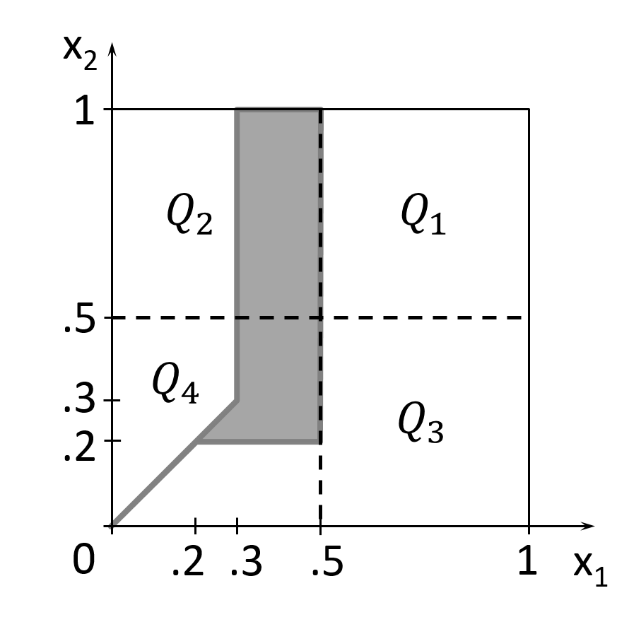
Figure 2: $(K,L)$-eigenvectors

Example 3.2

In this example, we take

$$B=\begin{pmatrix}.4&.5\\ .2&.5\end{pmatrix}$$ (22)

and consider the same $\lambda=.5$. To solve (1) for $A=B$ we need to solve the system

$$\max\bigl{(}\min(.4,x_{1}),\min(.5,x_{2})\bigr{)}=\min(.5,x_{1}),$$ (23)

$$\max\bigl{(}\min(.2,x_{1}),\min(.5,x_{2})\bigr{)}=\min(.5,x_{2})$$ (24)

Note that (24) is the same as (19). The solution set for (23) is

$$Y^{\prime}=\Bigl{\{}(x_{1},x_{2})\colon((x_{1}=x_{2}\leq.5)\vee(x_{2}\leq x_{1}\leq.4)\vee((x_{1}\geq.5)\wedge(x_{2}\geq.5))\Bigr{\}},$$ (25)

and the solution set for (24) is $Y^{\prime\prime}=X^{\prime\prime}$ expressed in (21). Solution sets $Y^{\prime}$ and $Y^{\prime\prime}$ and their intersection are depicted in Figure 3 (there are no “genuine” $(K,L)$-eigenvectors in this example).

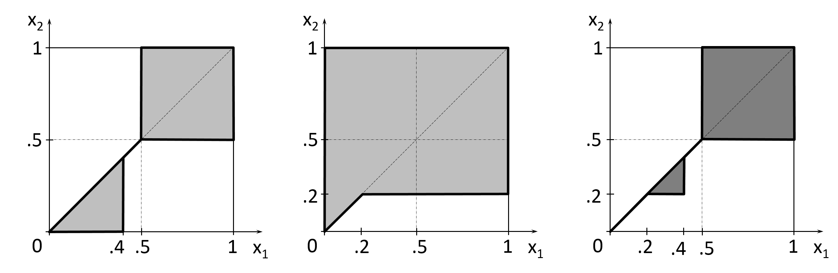
Figure 3: Sets $Y^{\prime}$ and $Y^{\prime\prime}$ and their intersection: the $0.5$-eigenspace of $B$

We are now going to give a theoretical description of background eigenvectors, principal eigenvectors and $(K,L)$-eigenvectors in max-min algebra.

3.1 Background $\lambda$-eigenvectors

These are the vectors that satisfy $Ax=\lambda\mathbf{1}$ and $x_{i}\geq\lambda$ for all $i$. Let us introduce the following notation:

$$\begin{split}N^{>\lambda}=\{k\colon\max\limits_{1\leq i\leq n}a_{ik}>\lambda\},\quad N^{\leq\lambda}=\{k\colon\max\limits_{1\leq i\leq n}a_{ik}\leq\lambda\}.\end{split}$$ (26)

The set of background eigenvectors can be described as follows.

Proposition 3.1

Let $A\in\mathbb{B}^{n\times n}$ and $\lambda\in\mathbb{B}$. Then the set of background $\lambda$-eigenvectors of $A$ is nonempty if and only if

$$\max\limits_{1\leq j\leq n}a_{ij}\geq\lambda\quad\forall i.$$ (27)

If (27) holds then the set of background eigenvectors is given by

$$\{x\colon x_{k}=\lambda\ \text{for $k\in N^{>\lambda}$},\lambda\leq x_{k}\leq 1\ \text{for $k\in N^{\leq\lambda}$}\}.$$ (28)

Proof: Observe first that if there exist $i$ with $a_{ij}<\lambda$ for all $j$, then also $a_{ij}x_{j}<\lambda$ for all $j$ implying that $\bigoplus_{j=1}^{n}a_{ij}x_{j}=\lambda$ cannot hold and the set of background eigenvectors is empty. If (27) holds then the constant vector $x=\lambda\mathbf{1}$ satisfies $Ax=\lambda\mathbf{1}$ hence the set of background eigenvectors is nonempty.

If $k\in N^{>\lambda}$ then there exists $i$ that $a_{ik}>\lambda$, and we need $x_{k}=\lambda$ to make sure that $\bigoplus_{j=1}^{n}a_{ij}x_{j}\leq\lambda$. This shows that the set of background $\lambda$-eigenvectors is a subset of (28).

Now take a vector from (28). Obviously, it satisfies $x_{i}\geq\lambda$ for each $i$. Since also $\max_{j}a_{ij}\geq\lambda$ for all $j$, we have $\bigoplus_{j}a_{ij}x_{j}\geq\lambda$. But we also have $\bigoplus_{j}a_{ij}x_{j}\leq\lambda$. Indeed, since $x_{j}=\lambda$ in (28) whenever $j\in N^{>\lambda}$, that is, whenever there exists $i$ with $a_{ij}>\lambda$, we have $a_{ij}x_{j}\leq\lambda$ for all such $j$ and all $i$. For $j\in N^{\leq\lambda}$, inequality $a_{ij}x_{j}\leq\lambda$ follows from $\max_{i}a_{ij}\leq\lambda$ (by the definition of $N^{\leq\lambda}$).

The proof is complete.  $\square$

Note that the set of background eigenvectors is a max-min convex set, and not a max-min space. The proof of the following corollary of Proposition 3.2 is straightforward and will be omitted.

Corollary 3.1

If the set of background eigenvectors is non-empty, then it is the max-min convex hull of $e^{\lambda 0}=\lambda\mathbf{1}$ and vectors $e^{\lambda k}$ for $k\in N^{\leq\lambda},$ for which

$$e^{\lambda k}_{i}=\begin{cases}1,&\text{if $k=i$,}\\ \lambda,&\text{otherwise.}\end{cases}$$

The following proposition will be helpful when describing more general sets of the form (28) as max-min convex hulls.

Proposition 3.2

Suppose that

$$S=\{x\colon x_{k}=\lambda\ \text{for $k\in N_{1}$},\ \lambda\leq x_{k}\leq 1\ \text{for $k\in N_{2}$}\},$$ (29)

where $N_{1}$ and $N_{2}$ are such that $N_{1}\cup N_{2}=N(=\{1,\ldots,n\})$ and $N_{1}\cap N_{2}=\emptyset$. Then

$$S=\{\lambda\mathbf{1}\oplus z_{N_{2}}\colon z_{N_{2}}\in\mathbb{B}^{|N_{2}|}\}$$ (30)

3.2 Principal $\lambda$-eigenvectors

These are the vectors that satisfy $Ax=x$ and $x_{i}\leq\lambda$ for all $i$. Description of a generating set of the space of principal max-min $\lambda$-eigenvectors is given below. Observe that any principal $\lambda$-eigenvector is a principal eigenvector and therefore we can apply Theorem 2.1.

Corollary 3.2 (Gondran-Minoux [18], Ch. 6, Corollary 3.5)

The set of principal $\lambda$-eigenvectors of $A\in\mathbb{B}^{n\times n}$ is the max-min column space $\{A^{*}_{\lambda}y\colon y\in\mathbb{B}^{n}\}$, where the columns of $A^{*}_{\lambda}$ are defined by

$$(A^{*}_{\lambda})_{\cdot i}=\lambda a_{ii}^{+}(A^{*})_{\cdot i}\colon i=1,\ldots,n.$$ (31)

More precisely, each vector of (31) is a principal $\lambda$-eigenvector, and each principal $\lambda$-eigenvector $x$ can be represented as

$$x=\bigoplus_{i\in C(A,x)}\lambda x_{i}a_{ii}^{+}(A^{*})_{\cdot i},$$ (32)

where $C(A,x)\subseteq N$ is a set containing a node from each strongly connected component of $\operatorname{Sat}(A,x)$.

Proof: The claim follows as an easy corollary of Theorem 2.1. Indeed, since $a_{ii}^{+}(A^{*})_{\cdot i}$ satisfies $Ax=x$, so does $\lambda a_{ii}^{+}(A^{*})_{\cdot i}$. As components of this vector do not exceed $\lambda$, it is a principal $\lambda$-eigenvector. Letting $x$ be a principal $\lambda$-eigenvector, we see that it satisfies (5) since it satisfies $Ax=x$. Equation (32) follows from (5) after multiplying both parts of (5) by $\lambda$ and observing that $\lambda x=x$ since $x_{i}\leq\lambda$ for all $i$.  $\square$

3.3 $(K,L)$ $\lambda$-eigenvectors

Now we consider $(K,L)$ max-min $\lambda$-eigenvectors, i.e., $x\in\mathbb{B}^{n}$ such that $Ax=\lambda x$, $x_{i}\leq\lambda$ for $i\in K$ and $x_{i}\geq\lambda$ for $i\in L$, where $K,L\subseteq\{1,\ldots,n\}$ are such that $K\cup L=\{1,\ldots,n\}$ and $K\cap L=\emptyset$.

By this definition, every $(K,L)$ $\lambda$-eigenvector is of the form $x=(x_{L}\ x_{K})$ (in a suitable permutation of indices ) with

$$A_{KK}x_{K}\oplus A_{KL}x_{L} =x_{K},\quad x_{K}\leq\lambda\mathbf{1}_{K}$$ (33)

$$A_{LK}x_{K}\oplus A_{LL}x_{L} =\lambda\mathbf{1}_{L},\quad x_{L}\geq\lambda\mathbf{1}_{L}$$ (34)

We start with describing the solvability and the set of solutions for (33).

Proposition 3.3

Equation (33) is solvable (together with $x_{K}\leq\lambda\mathbf{1}_{K}$) with respect to $x_{K}$ if and only if

$$(A_{KK})^{*}A_{KL}x_{L}\leq\lambda\mathbf{1}_{K},$$ (35)

and then the set of its solutions for fixed $x_{L}$ is given by

$$\begin{split}S_{K}(x_{L},\lambda)&=\{(A_{KK})^{*}A_{KL}x_{L}\oplus v\colon A_{KK}v=v,\ v\leq\lambda\mathbf{1}_{K}\}\\ &=\{(A_{KK})^{*}A_{KL}x_{L}\oplus(A_{KK})^{*}_{\lambda}z_{K}\colon z_{K}\in\mathbb{B}^{|K|}\}\end{split}$$ (36)

where $(A_{KK})^{*}_{\lambda}$ is defined as in (31).

Proof: the assertion follows from Theorem 2.2.  $\square$

Before describing the solvability of (34), denote

$$L_{1}=\{i\in L\colon\bigoplus_{j\in L}a_{ij}\geq\lambda\},\quad L_{2}=\{i\in L\colon\bigoplus_{j\in L}a_{ij}<\lambda\}$$ (37)

Proposition 3.4

Equation (34), considered together with $x_{K}\leq\lambda\mathbf{1}_{K}$, is equivalent to

$$A_{L_{1}L}x_{L} =\lambda\mathbf{1}_{L_{1}},\quad x_{L}\geq\lambda\mathbf{1}_{L},$$ (38)

$$A_{L_{2}K}x_{K} =\lambda\mathbf{1}_{L_{2}},\quad x_{K}\leq\lambda\mathbf{1}_{K}.$$ (39)

Proof: In terms of the notation (37), equation (34) is written as follows:

$$A_{L_{1}K}x_{K}\oplus A_{L_{1}L}x_{L}=\lambda\mathbf{1}_{L_{1}},$$ (40)

$$A_{L_{2}K}x_{K}\oplus A_{L_{2}L}x_{L}=\lambda\mathbf{1}_{L_{2}},$$ (41)

$$x_{L}\geq\lambda\mathbf{1}_{L},\quad x_{K}\leq\lambda\mathbf{1}_{K}.$$ (42)

We now show that (40), (41), (42) are equivalent to (38) and (39). Indeed, $x_{L}\geq\lambda\mathbf{1}_{L}$ together with $\bigoplus_{j\in L}a_{ij}\geq\lambda$ for $i\in L_{1}$ imply that $A_{L_{1}L}x_{L}\geq\lambda\mathbf{1}_{L_{1}}$ holds for any feasible $x$, and this makes the first term in (40) redundant, also since $x_{K}\leq\lambda\mathbf{1}_{K}$ implies $A_{L_{1}K}x_{K}\leq\lambda\mathbf{1}_{L_{1}}$. As for the second term in (41), we have $\bigoplus_{j\in L}a_{ij}<\lambda$ for $i\in L_{2}$ implying that $A_{L_{2}L}x_{L}<\lambda\mathbf{1}_{L_{2}}$ and making this term redundant as well.  $\square$

To solve (38) let us introduce the following notation in analogy with (26):

$$L^{>\lambda,L_{1}} =\{k\in L\colon\max\limits_{i\in L_{1}}a_{ik}>\lambda\}$$ (43)

$$L^{>\lambda,K} =\{\ell\in L\colon\max_{k\in K}((A_{KK})^{*}A_{KL})_{k\ell}>\lambda\}$$ (44)

$$L^{\prime} =L^{>\lambda,L_{1}}\cup L^{>\lambda,K},\quad\tilde{L}=L\backslash L^{\prime}.$$ (45)

Proposition 3.5

The solution set to (38) with condition (35) is given by

$$\begin{split}&S_{L}(\lambda)=\{\lambda\mathbf{1}_{L}\oplus z_{\tilde{L}}\colon z_{\tilde{L}}\in\mathbb{B}^{|\tilde{L}|}\}.\end{split}$$ (46)

Proof: Following Proposition 3.1, the set of solutions to (38) is

$$\{x_{L}\colon x_{\ell}=\lambda\ \text{for $\ell\in L^{>\lambda,L_{1}}$},\lambda\leq x_{\ell}\leq 1\ \text{for $\ell\notin L^{>\lambda,L_{1}}$}\}.$$ (47)

However, we also have (35), which is satisfied whenever

$$x_{\ell}=\lambda\text{ for all }\ell\in L^{>\lambda,K}.$$ (48)

The set of solutions to (38) with respect to both conditions (47) and (48) can be written as

$$S_{L}(\lambda)=\{x_{L}\colon x_{\ell}=\lambda\ \text{for $\ell\in L^{\prime}$},\lambda\leq x_{\ell}\leq 1\ \text{for $\ell\in\tilde{L}$}\}.$$ (49)

Using Proposition 3.2 we can express $S_{L}(\lambda)$ as shown in (46).  $\square$

Proposition 3.6

The set of vectors $x_{K}$ solving (33) for a given $x_{L}=\lambda\mathbf{1}_{L}\oplus z_{\tilde{L}}$ is of the form

$$\begin{split}&S_{K}(x_{L},\lambda)=\{\lambda(A_{KK})^{*}A_{KL}\mathbf{1}_{L}\oplus(A_{KK})^{*}A_{K\tilde{L}}z_{\tilde{L}}\oplus(A_{KK})^{*}_{\lambda}z_{K}\colon z_{K}\in\mathbb{B}^{|K|}\}.\end{split}$$ (50)

Proof: The computation of $S_{K}(x_{L},\lambda)$ in view of (36) uses $x_{L}\in S_{L}(\lambda)$ according to (46) and distributivity.

$$\begin{split}&S_{K}(x_{L},\lambda)=\{(A_{KK})^{*}A_{KL}x_{L}\oplus(A_{KK})^{*}_{\lambda}z_{K}\colon z_{K}\in\mathbb{B}^{|K|}\}\\ &=\{\lambda(A_{KK})^{*}A_{KL}\mathbf{1}_{L}\oplus(A_{KK})^{*}A_{K\tilde{L}}z_{\tilde{L}}\oplus(A_{KK})^{*}_{\lambda}z_{K}\colon z_{K}\in\mathbb{B}^{|K|}\}.\end{split}$$ (51)

$\square$

Substituting $x_{K}\in S_{K}(x_{L},\lambda)$ given by (50) into (39), we obtain the following equation:

$$\lambda A_{L_{2}K}(A_{KK})^{*}A_{KL}\mathbf{1}_{L}\oplus A_{L_{2}K}(A_{KK})^{*}A_{K\tilde{L}}z_{\tilde{L}}\oplus A_{L_{2}K}(A_{KK})^{*}_{\lambda}z_{K}=\lambda\mathbf{1}_{L_{2}}$$ (52)

It can be seen that the system (52) is of the form $A^{\prime}z^{\prime}\oplus b^{\prime}=\lambda\mathbf{1}$ where

$$\begin{split}A^{\prime}&=(A_{L_{2}K}(A_{KK})^{*}A_{K\tilde{L}},\ A_{L_{2}K}(A_{KK})^{*}_{\lambda}),\\ b^{\prime}&=\lambda A_{L_{2}K}(A_{KK})^{*}A_{KL}\mathbf{1}_{L},\ z^{\prime}=(z_{\tilde{L}}\ z_{K})^{T}.\end{split}$$ (53)

This observation enables us to describe the solution $z^{\prime}=(z_{\tilde{L}}\ z_{K})^{T}$ using the results of Subsection 2.2, as below.

Proposition 3.7

The minimal solutions $(z^{\prime})^{W}=(z_{K}^{W}z_{\tilde{L}}^{W})$ of $A^{\prime}z^{\prime}\oplus b^{\prime}=\lambda\mathbf{1}$ with $A^{\prime}$ and $b^{\prime}$ as in (53) are defined by

$$(z^{\prime})^{W}_{j}=\begin{cases}\lambda,&\text{if $j\in W$},\\ 0,&\text{otherwise}.\end{cases}$$ (54)

where $\{\cup C_{j}\colon j\in W\}$ with

$$C_{j}=\{i\in I_{0}\colon(A^{\prime})_{ij}=\lambda\}\quad\text{for $j\in\tilde{N}$},$$ (55)

is a minimal covering of

$$I_{0}=\{i\in L_{2}\colon A_{iK}(A_{KK})^{*}A_{KL}\mathbf{1}_{L}<\lambda\}.$$ (56)

Proposition 3.8

The set of all solutions of $A^{\prime}z^{\prime}\oplus b^{\prime}=\lambda\mathbf{1}$ with $A^{\prime}$ and $b^{\prime}$ as in (53) is given by $\cup_{W}S_{W}$ where the union is taken over all minimal coverings $\{\cup C_{j}\colon j\in W\}$ of $I_{0}$ and $S_{W}=\{z^{W}\oplus v_{\tilde{N}}\colon v_{\tilde{N}}\in\mathbb{B}^{|\tilde{N}|}\}$

Proof:[Proof of Proposition 3.7 and 3.8] Observe that all entries of $A_{KK}^{*}A_{K\tilde{L}}$ do not exceed $\lambda$ by (44) and the definition of $\tilde{L}$, and that all coefficients of $(A_{KK})^{*}_{\lambda}$ do not exceed $\lambda$ by (31). Hence the entries of $A^{\prime}$ and $b^{\prime}$ do not exceed $\lambda$, and all solutions of $A^{\prime}z^{\prime}\oplus b^{\prime}=\lambda\mathbf{1}$ can be found as in Corollary 2.1 and using (16), with $A^{\prime}$ and $b^{\prime}$ instead of $A$ and $b$, $\tilde{N}=\tilde{L}\cup K$ instead of $N$.  $\square$

The next theorem, which describes the set of $(K,L)$ $\lambda$-eigenvectors, is the main result of the section. This theorem follows from the arguments written above, but we also include a formal proof based on backtracking the above arguments.

Theorem 3.1

Let $A\in\mathbb{B}^{n\times n}$, $\lambda\in\mathbb{B}$ and $K,L$ such that $K\cup L=N$ and $K\cap L=\emptyset$ be given. Then $(K,L)$-eigenvector exists if and only if (52) is solvable, which happens if and only if $I_{0}=\cup_{j\in\tilde{N}}C_{j}$, with $I_{0}$ and $C_{j}$ defined as in (55) and (56) and $\tilde{N}=\tilde{L}\cup K$.

In this case, $x=(x_{K}\ x_{L})^{T}$ is a $(K,L)$-eigenvector of $A$ with eigenvalue $\lambda$ if and only if $x_{K}$ and $x_{L}$ can be expressed as follows:

$$\begin{split}x_{L}&=\lambda\mathbf{1}_{L}\oplus v_{\tilde{L}},\\ x_{K}&=\lambda(A_{KK})^{*}A_{KL}\mathbf{1}_{L}\oplus(A_{KK})^{*}A_{K\tilde{L}}v_{\tilde{L}}\oplus(A_{KK})^{*}_{\lambda}(z_{K}^{W}\oplus v_{K}),\end{split}$$ (57)

where $v_{K}\in\mathbb{B}^{|K|},$ $v_{\tilde{L}}\in\mathbb{B}^{|\tilde{L}|},$ and $z^{W}$ is the minimal solution of (52) corresponding to a minimal covering $\{C_{j}\colon j\in W\}$ of $I_{0}$.

Proof: Consider a set of vectors $z_{\tilde{N}}=(z_{K}\ z_{\tilde{L}})$ described by

$$z_{K}=z_{K}^{W}\oplus v_{K},\quad z_{\tilde{L}}=z_{\tilde{L}}^{W}\oplus v_{\tilde{L}},\quad v_{K}\in\mathbb{B}^{|K|},\quad v_{\tilde{L}}\in\mathbb{B}^{|\tilde{L}|}$$

for a minimal $W$ such that $\cup_{j\in W}C_{j}=I_{0}$. By Proposition 3.7 and Proposition 3.8, the union of these sets over $W$ comprises the set of all solutions to (52), which is solvable if and only if $\cup_{j\in\tilde{N}}C_{j}=I_{0}$.

Equation (52), if it is solvable, is the same as $A_{L_{2}K}x_{K}=\lambda\mathbf{1}_{L_{2}}$ of (39), where $x_{K}\in S_{K}(x_{L},\lambda)$ with the latter set described in (50). Note that the condition $x_{K}\leq\lambda\mathbf{1}_{K}$ immediately follows from (50). Then we see that (57) describes all vectors $(x_{K}\ x_{L})$ such that $x_{L}\in S_{L}(\lambda)$, $x_{K}\in S_{K}(x_{L},\lambda)$ and condition (39) is satisfied, after observing that $x_{L}=\lambda\mathbf{1}_{L}\oplus z^{W}_{\tilde{L}}\oplus v_{\tilde{L}}=\lambda\mathbf{1}\oplus v_{\tilde{L}}$ (since each component of $z^{W}$ is less than or equal to $\lambda$).

By Proposition 3.6, $S_{K}(x_{L},\lambda)$ is the set of all vectors $x_{K}$ solving (33) for a given $x_{L}=\lambda\mathbf{1}_{L}\oplus z_{\tilde{L}}$, which is by Proposition 3.5 a general solution to (38) with condition (35). Observe that by Proposition 3.3 condition (35) is equivalent to solvability of (33) with respect to $x_{K}$ for a given $x_{L}$. Thus (57) describes all vectors $(x_{K}\ x_{L})$ that satisfy (33), (38) and (39) simultaneously.

Furthermore, in view of Proposition 3.4, (38) and (39) can be replaced by (34), implying that  (57) yields all solutions to (33) and (34) if (52) is solvable.

If (52) is not solvable then (39) is not compatible with (33) and (38). The proof is complete.  $\square$

Let us also note the following special case of the above considerations.

Corollary 3.3

If $L_{2}=\emptyset$ then the solution set to (33), (34) is the set of $x=(x_{L}\ x_{K})$ given by

$$\begin{split}x_{L}&=\lambda\mathbf{1}_{L}\oplus z_{\tilde{L}},\\ x_{K}&=\lambda(A_{KK})^{*}A_{KL}\mathbf{1}_{L}\oplus(A_{KK})^{*}A_{K\tilde{L}}z_{\tilde{L}}\oplus(A_{KK})^{*}_{\lambda}z_{K},\end{split}$$ (58)

where parameters $z_{\tilde{L}}\in\mathbb{B}^{|\tilde{L}|},\ z_{K}\in\mathbb{B}^{|K|}$ have arbitrary values.

In this case (52) is trivially solvable, as an “empty equation”.

Theorem 3.1 gives us a clear way to generate all $(K,L)$-eigenvectors. If we want to ”test” its validity, we may recall that, since it can be easily shown that $Ax\leq x$ and $A^{*}x=x$ are equivalent [18] and since any $\lambda$-eigenvector satisfies $Ax=\lambda x\leq x$, we should have $A^{*}x=x$ for any $\lambda$-eigenvector $x$. Let us show that any vector given by (57) satisfies this property.

Corollary 3.4

Let $x=(x_{K}\ x_{L})$ satisfy (57). Then we have $A^{*}x=x$.

Proof: Since $A^{*}x=x$ is equivalent to $Ax\leq x$, we will prove the latter. Inequality $Ax\leq x$ can be written as the following four:

$$A_{KK}x_{K}\leq x_{K},\ A_{KL}x_{L}\leq x_{K},\ A_{LK}x_{K}\leq x_{L},\ A_{LL}x_{L}\leq x_{L}.$$

The inequality $A_{KK}x_{K}\leq x_{K}$ follows since $x_{K}$, by the second equation of (57), satisfies $(A_{KK})^{*}v=x_{K}$ for some $v$ and we have $A_{KK}(A_{KK})^{*}=(A_{KK})^{+}\leq(A_{KK})^{*}$. As for the inequality $A_{KL}x_{L}\leq x_{K}$, we have

$$A_{KL}x_{L}=\lambda A_{KL}\mathbf{1}_{L}\oplus A_{K\tilde{L}}v_{\tilde{L}}\leq x_{K}.$$

As for the inequality $A_{LK}x_{K}\leq x_{L}$, it follows since $x_{L}$ and $x_{K}$ of  (57) satisfy $x_{L}\geq\lambda\textbf{1}$ and $x_{K}\leq\lambda\textbf{1}$.

It remains to prove the inequality $A_{LL}x_{L}\leq x_{L}$, which we are going to do for arbitrary $x_{L}$ belonging to the set defined in (47), using that this set contains (46) and hence any $x_{L}$ given by the first equation of (57). Denoting $L_{3}=L^{>\lambda,L_{1}}$ and $L_{4}=L\backslash L^{>\lambda,L_{1}}$ and seeing that $x_{L_{3}}=\lambda\mathbf{1}_{L_{3}}$ and $x_{L_{4}}\geq\lambda\mathbf{1}_{L_{4}}$, we have to prove

$$\lambda A_{L_{3}L_{3}}\textbf{1}_{L_{3}}\leq\lambda\textbf{1}_{L_{3}},\ A_{L_{3}L_{4}}x_{L_{4}}\leq\lambda\textbf{1}_{L_{3}},\ \lambda A_{L_{4}L_{3}}\textbf{1}_{L_{3}}\leq x_{L_{4}},\ A_{L_{4}L_{4}}x_{L_{4}}\leq x_{L_{4}}.$$

The first and the third of these inequalities are obvious. As for the inequalities $A_{L_{3}L_{4}}x_{L_{4}}\leq\lambda\textbf{1}_{L_{3}}$ and $A_{L_{4}L_{4}}x_{L_{4}}\leq x_{L_{4}}$, we observe using the definition of $L^{>\lambda,L_{1}}$ (43) and $L_{2}$ in (37) that all entries in $A_{LL_{4}}$ do not exceed $\lambda$, and recall that $x_{L_{4}}\geq\lambda\textbf{1}_{L_{4}}$. Thus the inequality $A_{LL}x_{L}\leq x_{L}$ also follows and the proof is complete.  $\square$

Let us now describe the set of $(K,L)$-eigenvectors as a max-min convex hull of a finite number of points.

Corollary 3.5

If the set of $(K,L)$-eigenvectors associated with eigenvalue $\lambda$ is non-empty, then it is the max-min convex hull of the points $x^{W,0}=(x_{K}^{W,0}\;x_{L}^{W,0})$, $x^{W,i}=(x_{K}^{W,i}\;x_{L}^{W,i})$ for $i\in\tilde{L}$ and $x^{W,k}=(x_{K}^{W,k}\;x_{L}^{W,k})$ for $k\in K$, where

$$\begin{split}x_{L}^{W,0}&=\lambda\mathbf{1}_{L},\quad x_{K}^{W,0}=(A_{KK})^{*}A_{KL}x_{L}^{W,0}\oplus(A_{KK})^{*}_{\lambda}z_{K}^{W},\\ x_{L}^{W,i}&=\lambda\mathbf{1}_{L}\oplus e_{i},\quad x_{K}^{W,i}=(A_{KK})^{*}A_{KL}x_{L}^{W,i}\oplus(A_{KK})^{*}_{\lambda}z_{K}^{W},\\ x_{L}^{W,k}&=\lambda\mathbf{1}_{L},\quad x_{K}^{W,k}=(A_{KK})^{*}A_{KL}x_{L}^{W,k}\oplus(A_{KK})^{*}_{\lambda}(z_{K}^{W}\oplus e_{k}),\end{split}$$ (59)

and $W$ ranges over all minimal coverings $\{C_{j}\colon j\in W\}$ of $I_{0}$.

Proof: Using that $\mathbb{B}^{|\tilde{N}|}=\mathbb{B}^{|K|}\times\mathbb{B}^{|\tilde{L}}|$ is a max-min convex set generated by the zero vector $\mathbf{0}$ and unit vectors $e_{i}$ for $i\in\tilde{L}$ and $e_{k}$ for $k\in K$, we substitute these generators for $v_{\tilde{N}}=(v_{\tilde{L}}\ v_{K})$ in (57) and obtain that the set of $(K,L)$-eigenvectors is the max-min convex hull of the points described by (59).  $\square$

For the purposes of computation note that the minimal solutions of (52), which correspond to minimal coverings of $I_{0}$ (56) by unions of $C_{j}$ (55), can be found using the methods described in Elbassioni [9]. The set of all $(K,L)$-eigenvectors can be then efficiently described using Theorem 3.1 and Corollary 3.5.

In particular, the number of minimal solutions of $A^{\prime}z^{\prime}\oplus b^{\prime}=\lambda\mathbf{1}$ is equal to the number of minimal coverings $\{\cup C_{j}\colon j\in W\}$ of $I_{0}$, which depends on entries of $A$ (particularly $(A_{KK})^{*}$) and given $\lambda$. However, the dependency of the points generating the set of $(K,L)$-eigenvectors as their max-min convex hull on these minimal coverings seems rather uncertain and can be eliminated if $A_{KK})^{*}_{\lambda}z_{K}^{W}$ is dominated by the sum of other terms in (57).

In the following example, there is just one possible minimal covering that produces the only minimal solution used in further computation.

Example 3.3

The following three-dimensional example shows how to find the eigenspace for given matrix $A$ and eigenvalue $\lambda$.

Take

$$A=\begin{pmatrix}.1&.5&.7\\ 0&.4&.8\\ .1&.1&.5\end{pmatrix},\ \lambda=.5$$

First, let us introduce the notation of the vector with interval entries. The vector where entries are of form $a\leq x_{1}\leq b$ and $c\leq x_{2}\leq d$ is denoted in further text as

$$x=\begin{pmatrix}\langle a,b\rangle\\ \langle c,d\rangle\end{pmatrix}.$$

As the $\lambda$-eigenspace is a union of background, principal and $(K,L)$ $\lambda$-eigenvectors, we are going to compute the solution for each individual case.

For the case of background $\lambda$-eigenvectors, first, we have to verify the existence of this eigenvector-type. From (27) we see that this set is nonempty. According to (28), background eigenvectors are all vectors of form

$$x=\begin{pmatrix}\langle.5,1\rangle\\ \langle.5,1\rangle\\ .5\end{pmatrix}$$ (60)

Their set is the max-min convex hull of $(.5,.5,.5),$ $(1,.5,.5),$ $(.5,1,.5)$.

Principal $\lambda$-eigenvectors are computed using Corollary 3.2. We find that generators of max-min eigenspace for $x_{i}\leq\lambda$ for all $i$ are $(.1,.1,.1)$, $(.4,.4,.1)$ and $(.5,.5,.5)$. Of these vectors, the first one is obviously redundant as $(.1,.1,.1)=.1\otimes(.5,.5,.5)$. If we want to describe this eigenspace as a max-min convex hull then the zero vector $(0,0,0)$ is routinely added to the generating set.

When computing $(K,L)$ eigenvectors, first we have to determine particular $(K,L)$ partition. For partition $K=\{1,3\}$, $L=\{2\}$ we have

$$A_{KK}=\begin{pmatrix}.1&.7\\ .1&.5\end{pmatrix},A_{KL}=\begin{pmatrix}.5\\ .1\end{pmatrix},A_{LK}=\begin{pmatrix}0&.8\end{pmatrix},A_{LL}=\begin{pmatrix}.4\end{pmatrix},$$

$$\ (A_{KK})^{*}=\begin{pmatrix}1&.7\\ .1&1\end{pmatrix},\ (A_{KK})_{\lambda}^{*}=\begin{pmatrix}.1&.5\\ .1&.5\end{pmatrix}.$$

We are solving the system

$$\begin{pmatrix}.1&.7\\ .1&.5\end{pmatrix}\otimes\begin{pmatrix}x_{1}\\ x_{3}\end{pmatrix}\oplus\begin{pmatrix}.5\\ .1\end{pmatrix}\otimes x_{2} =\begin{pmatrix}x_{1}\\ x_{3}\end{pmatrix}$$ (61)

$$\begin{pmatrix}0&.8\end{pmatrix}\otimes\begin{pmatrix}x_{1}\\ x_{3}\end{pmatrix}\oplus\begin{pmatrix}.4\end{pmatrix}\otimes x_{2} =\lambda$$ (62)

By verifying (35), we find out that(35) holds for all values $x_{2}$, and thus a solution to (61) exists.

We can also express the sets $L_{1}=\emptyset,L_{2}=\{2\},L^{\prime}=\emptyset$ and $\tilde{L}=\{2\}$. As $L_{2}\neq\emptyset$, we need to find the solution set to (52):

$$.5\otimes\begin{pmatrix}0&.8\end{pmatrix}\otimes\begin{pmatrix}1&.7\\ .1&1\end{pmatrix}\otimes\begin{pmatrix}.5\\ .1\end{pmatrix}\otimes 1\oplus\hskip 147.0pt$$

$$\begin{pmatrix}0&.8\end{pmatrix}\otimes\begin{pmatrix}1&.7\\ .1&1\end{pmatrix}\otimes\begin{pmatrix}.5\\ .1\end{pmatrix}\otimes 1\otimes z_{2}\oplus\begin{pmatrix}0&.8\end{pmatrix}\otimes\begin{pmatrix}.1&.5\\ .1&.5\end{pmatrix}\otimes\begin{pmatrix}z_{1}\\ z_{3}\end{pmatrix}=.5,$$ (63)

which is the same as

$$.1\oplus\begin{pmatrix}.1&.1&.5\end{pmatrix}\otimes\begin{pmatrix}z_{1}\\ z_{2}\\ z_{3}\end{pmatrix}=.5$$ (64)

The only minimal (and hence the least) solution to this system is $z^{\{3\}}=(0,0,.5)$, so the solution set is $\{z\colon z^{\{3\}}\leq z\leq 1\}$. We can also express $z_{\tilde{L}}^{\{3\}}=z_{L}^{\{3\}}=(0)$, $z_{K}^{\{3\}}=(0,.5)$.

Following Theorem 3.1 and using equations (57) we obtain

$$\begin{split}x_{2}&=.5\oplus v_{2},\\ \begin{pmatrix}x_{1}\\ x_{3}\end{pmatrix}&=.5\begin{pmatrix}1&.7\\ .1&1\end{pmatrix}\begin{pmatrix}.5\\ .1\end{pmatrix}\oplus\begin{pmatrix}1&.7\\ .1&1\end{pmatrix}\begin{pmatrix}.5\\ .1\end{pmatrix}v_{2}\\ &\oplus\begin{pmatrix}.1&.5\\ .1&.5\end{pmatrix}\Biggl{(}\begin{pmatrix}0\\ .5\end{pmatrix}\oplus\begin{pmatrix}v_{1}\\ v_{3}\end{pmatrix}\Biggl{)}\\ &=\begin{pmatrix}.5\\ .1\end{pmatrix}(1\oplus v_{2})\oplus\begin{pmatrix}.5\\ .5\end{pmatrix}=\begin{pmatrix}.5\\ .5\end{pmatrix},\end{split}$$ (65)

which can be written as

$$x=\begin{pmatrix}.5\\ \langle.5,1\rangle\\ .5\end{pmatrix}$$ (66)

For the partition $K=\{2,3\}$, $L=\{1\}$ we are solving the system

$$\begin{pmatrix}.4&.8\\ .1&.5\end{pmatrix}\otimes\begin{pmatrix}x_{2}\\ x_{3}\end{pmatrix}\oplus\begin{pmatrix}0\\ .1\end{pmatrix}\otimes x_{1} =\begin{pmatrix}x_{2}\\ x_{3}\end{pmatrix}$$ (67)

$$\begin{pmatrix}.5&.7\end{pmatrix}\otimes\begin{pmatrix}x_{2}\\ x_{3}\end{pmatrix}\oplus\begin{pmatrix}.1\end{pmatrix}\otimes x_{1} =\lambda$$ (68)

Similarly to previous procedures we compute eigenvectors for this partition

$$x=\begin{pmatrix}\langle.5,1\rangle\\ .5\\ .5\end{pmatrix}$$ (69)

Thus we see that $(K,L)$-eigenvectors for $L=\{1\}$ and $L=\{2\}$ are background eigenvectors. By similar routine calculations we can check that the same is true for $(K,L)$-eigenvectors for any non-empty $L$, and this is different from Example 3.1, where we have $(K,L)$-eigenvectors that are neither background nor principal. Note that in Example 3.3 any set of $(K,L)$-eigenvectors is non-empty, as $(.5,.5,.5)$ is a $\lambda$-eigenvector, which is shared between all of them.

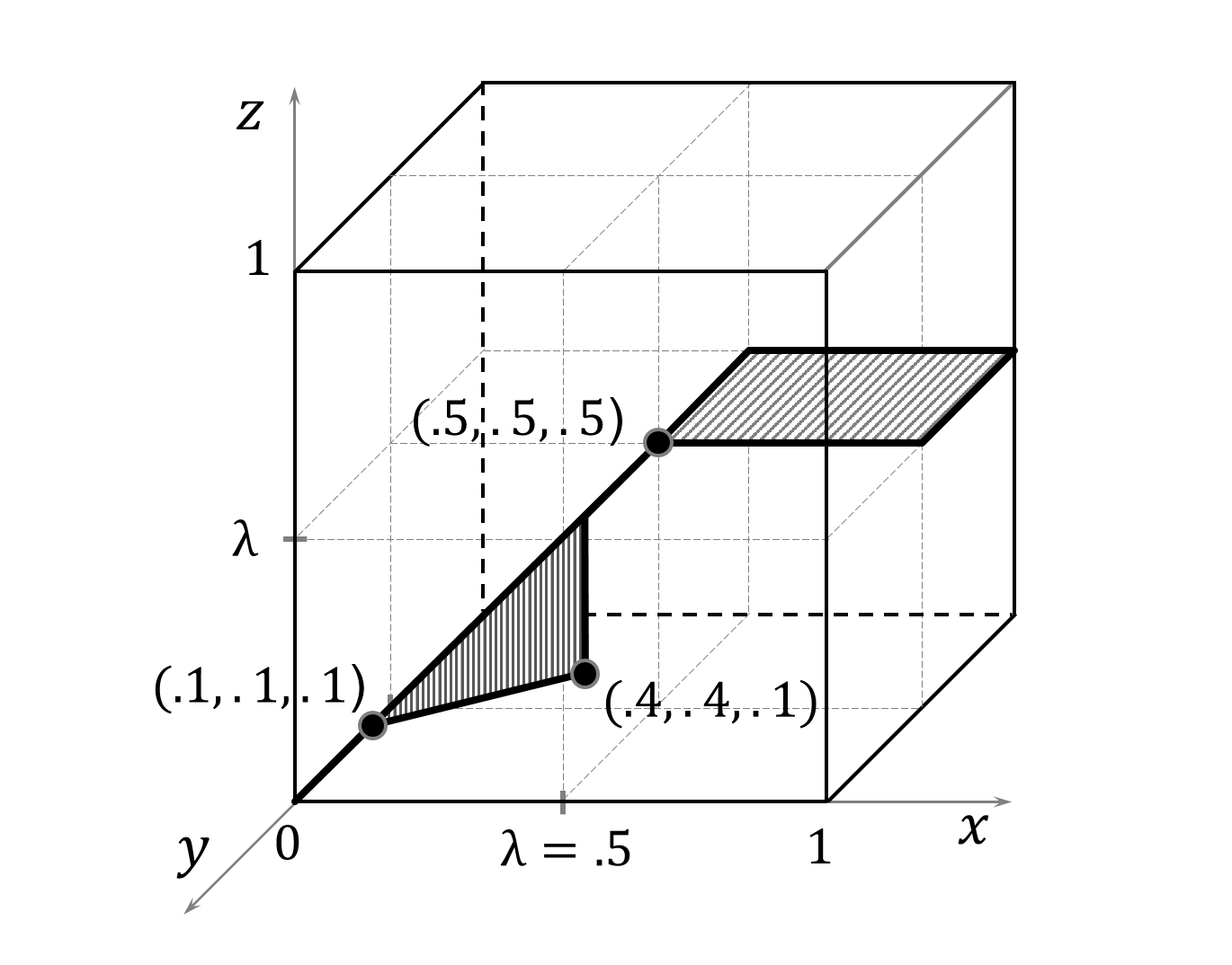
Figure 4: Eigenspace for $A$ and $\lambda$ of Example 3.3

The whole $\lambda$-eigenspace, shown on Figure 4, is thus the union of two parts: principal eigenvectors and background eigenvectors. This eigenspace (as a union of max-min convex hulls which is itself max-min convex) is the max-min convex hull of: $(.5,.5,.5)$, $(1,.5,.5)$, $(.5,1,.5)$, $(.4,.4,.1)$ and $(0,0,0)$. Removing the zero vector we obtain a generating set of the whole $\lambda$-eigenspace, and next we notice that $(.5,.5,.5)$ is redundant, since for example $(.5,.5,.5)=.5\otimes(1,.5,.5)$. Thus the $\lambda$-eigenspace is generated by $(1,.5,.5)$, $(.5,1,.5)$ and $(.4,.4,.1)$.

4 Discussion

Theorem 3.1 and Corollary 3.5 provide us with a description of the sets of $(K,L)$-eigenvectors associated with eigenvalue $\lambda$ and, in particular, give us a finite set of points such that the set of $(K,L)$ max-min eigenvectors appears as the max-min convex hull of them. Collecting such points for all sets of $(K,L)$-eigenvectors we obtain a finite set of generators for the whole $\lambda$-eigenspace.

There are some problems with this description. Clearly, there are exponentially many partitions $K\cup L=\{1,\ldots,n\}$, and to implement the above described method for finding the generators of $\lambda$-eigenspace one should find a way to quickly eliminate many partitions that are redundant: in two of the three examples that we considered, only the trivial partitions, corresponding to principal and background eigenvectors, were important. The procedure also raises the question about the number of points that generate the $\lambda$-eigenspace. From Example 3.2, it is clear that the number of such points can exceed the dimension, as the eigenspace in this example is generated by $(.4,.2)$, $(.5,1),$ $(1,.5)$ (e.g., consider it as a “max-min quadrangle” between these points and the zero vector, and use the forms of max-min segments given in [24]), with none of these points being redundant. However, it is not known how quickly the minimal number of such generators can grow with matrix dimension.

Similar questions can be asked also about the set of $(K,L)$-eigenvectors. The points that generate this set as their max-min convex hull come from certain minimal coverings, whose number may also grow quickly with matrix dimension, unless $L_{2}=\emptyset$ as in Corollary 3.3. However, we have seen that the terms coming from these minimal coverings are often dominated by other terms, thus decreasing the number of points making up the max-min convex hull.

There is a perspective to develop an application of max-min $\lambda$-eigenspaces in medical diagnostics following the ideas of Sanchez [27]. Also, there are still many unresolved questions in the geometry over max-min semiring: about the generating sets of max-min eigenspaces and more general max-min linear spaces, and more generally, about max-min polytopes.

5 Acknowledgements

We thank our anonymous referees for their careful reading and constructive criticism, which helped to improve the paper.

References

• [1] F.L. Baccelli, G. Cohen, G.J. Olsder and J.P. Quadrat. Synchronization and Linearity. John Wiley and Sons, New York, 1992.
• [2] P. Butkovič. Max-Linear Systems: Theory and Algorithms. Springer, London, 2010.
• [3] P. Butkovič, H. Schneider, and S. Sergeev. Z-matrix equations in max-algebra, nonnegative linear algebra and other semirings. Linear and Multilinear Alg., 60(10):1191–1210, 2012.
• [4] Z.-Q. Cao, K.H. Kim, and F.W. Roush. Incline Algebra and its Applications. Chichester, 1984.
• [5] B.A. Carré. An algebra for network routing problems. J. of the Inst. of Maths. and Applics, 7, 1971.
• [6] K. Cechlárová. Eigenvectors in bottleneck algebra. Linear Algebra and its Applications, 175:63-73, 1992.
• [7] K. Cechlárová. A note on unsolvable systems of max–min (fuzzy) equations. Linear Algebra and its Applications, 310:123-128, 2000.
• [8] R. A. Cuninghame-Green, K. Cechlárová. Residuation in fuzzy algebra and some applications. Fussy Sets and Systems, 71(2):227-239, 1995.
• [9] K. Elbassioni. A note on systems with max-min and max-product constraints. Fuzzy Sets and Systems, 159, 2008, 2272-2277.
• [10] M. Gavalec. Monotone eigenspace structure in max-min algebra, Linear Algebra and its Applications, 345, 2002, 149-167.
• [11] M. Gavalec and Z. Němcová. Steady states of max-Łukasiewicz fuzzy systems, Fuzzy Sets and Systems, 325, 2017, 58-68.
• [12] M. Gavalec, Z. Němcová, S. Sergeev. Tropical linear algebra with the Łukasiewicz T-norm, Fuzzy Sets and Systems, 276, 2015, 131-148.
• [13] M. Gavalec, J. Plavka, D. Ponce. Strong tolerance of interval eigenvectors in fuzzy algebra, Fuzzy Sets and Systems, 369, 2019, 145-156.
• [14] M. Gavalec, J. Plavka, H. Tomášková. Interval eigenproblem in max-–min algebra, Linear Algebra and its Applications, 440, 2014, 24-33.
• [15] M. Gondran. Valeurs propres et vecteurs propres en classification hiérarchique, R.A.I.R.O. Informatique Théorique, 10(3), 1976, 39-46.
• [16] M. Gondran and M. Minoux. Valeurs propres et vecteurs propres en théorie des graphes, in Colloques Internationaux, C.N.R.S., Paris 1978, pp. 181-183.
• [17] M. Gondran and M. Minoux. Dioïds and Semirings: Links to fuzzy sets and other applications. Fuzzy Sets and Systems, 158, 2007, 1273–1294.
• [18] M. Gondran and M. Minoux. Graphs, Dioids and Semirings: New Applications and Algorithms. Springer, 2008.
• [19] E.P. Klement, R. Mesiar, and E. Pap. Triangular Norms. Kluwer Academic Publ., Dordrecht, 2000.
• [20] N. K. Krivulin. On solution of generalized linear vector equations in idempotent algebra. Vestnik St.-Petersburg Univ. Math., 39, 2006, 16–26.
• [21] N. K. Krivulin. Methods of idempotent algebra in the problems of modeling and analysis of complex systems. St.-Petersburg Univ. Publ., 2009. (in Russian)
• [22] G. L. Litvinov and V. P. Maslov. The correspondence principle for idempotent calculus and some computer applications. In J. Gunawardena (ed.) Idempotency, Cambridge Univ. Press, 1998, pages 420-443.
• [23] V. Nitica and S. Sergeev. Tropical convexity over max-min semiring. In G. L. Litvinov and S. N. Sergeev (eds.) Tropical and Idempotent Mathematics and Applications, vol. 616 of Cont. Math. series, American Mathematical Society, 2014, pages 241-260.
• [24] V. Nitica and S. Sergeev. On the dimension of max-min convex sets. Fuzzy Sets and Systems, 271, 2015, 88-101.
• [25] H. Nobuhara, B. Bede and K. Hirota. On various eigen fuzzy sets and their application to image reconstruction. Information Sciences 176, 2006, 2988-3010.
• [26] E. Rakus-Andersson, Fuzzy and Rough Techniques in Medical Diagnosis and Medication, vol. 212 of StudFuzz series, Springer, Berlin, 2007.
• [27] E. Sanchez. Resolution of eigen fuzzy sets equations. Fuzzy Sets and Systems 1(1), 1978, 69–74.
• [28] E. Sanchez. Eigen fuzzy sets and fuzzy relations. J. of Math. Analysis and Appl. 81, 1981, 399–421.