Differential Evolution Algorithm Aided Turbo Channel Estimation and Multi-User Detection for G.Fast Systems in the Presence of FEXT

Abstract

The ever-increasing demand for broadband Internet access has motivated the further development of the digital subscriber line to the G.fast standard in order to expand its operational band from 106 MHz to 212 MHz. Conventional far-end crosstalk (FEXT) based cancellers falter in the upstream transmission of this emerging G.fast system. In this paper, we propose a novel differential evolution algorithm (DEA) aided turbo channel estimation (CE) and multi-user detection (MUD) scheme for the G.fast upstream including the frequency band up to 212 MHz, which is capable of approaching the optimal Cramer-Rao lower bound of the channel estimate, whilst approaching the optimal maximum likelihood (ML) MUD’s performance associated with perfect channel state information, and yet only imposing about 5% of its computational complexity. Explicitly, the turbo concept is exploited by iteratively exchanging information between the continuous value-based DEA assisted channel estimator and the discrete value-based DEA MUD. Our extensive simulations show that 18 dB normalized mean square error gain is attained by the channel estimator and 10 dB signal-to-noise ratio gain can be achieved by the MUD upon exploiting this iteration gain. We also quantify the influence of the CE error, of the copper length and of the impulse noise. Our study demonstrates that the proposed DEA aided turbo CE and MUD scheme is capable of offering near-capacity performance at an affordable complexity for the emerging G.fast systems.

I Introduction

The demand for high-speed broadband Internet access has motivated the construction of the hybrid digital subscriber line (DSL) and optical fiber infrastructure, which has been standardized as G.fast by the International Telecommunication Union Telecommunication Standardization Sector (ITU-T) [1]. G.fast still relies on the copper access network and in-premises wiring for its last hundred meters, because it is prohibitively expensive to replace copper by optical fiber. The G.fast standard has already exploited a broad spectrum spanning up to 106 MHz, while the band up to 212 MHz has been planed for future broadband access [2, 3]. However, exploiting the spectrum beyond 30 MHz inevitably imposes significant electromagnetic coupling between the neighboring twisted-pairs, which is referred to as crosstalk. There are two types of crosstalk, depending on the specific source of coupling. Explicitly, coupling originating from transmitter co-located with a receiver is called near-end crosstalk (NEXT), while the coupling arriving from the opposite side of the duplex link is known as far-end crosstalk (FEXT) [4]. NEXT can be avoided by employing frequency duplexing division and transmission synchronization for separating the downstream and upstream transmissions [4], or by vectoring the source signals for the sake of increasing the total throughput of the cable [5]. By contrast, FEXT remains a significant impairment that hampers achieving high data rates for G.fast systems [1].

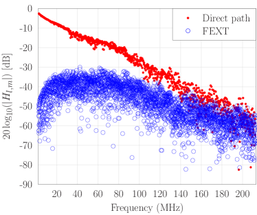
(a)                                                                     (b)

Figure 1: (a) Measured direct channel and crosstalk channel strengths, and (b) the average noise power amplified by the ZF FEXT canceller.

I-A Existing solutions for mitigating FEXT in the downstream

FEXT is generally mitigated by using spectrum shaping and vectoring [6] in the downstream transmission. The vectoring technique has also been standardized in G.993.5 by the ITU-T [7] and it was further developed with the objective of approaching Gigabit rates [1]. More specifically, in the downstream, the transmitters are co-located at the central office (CO) or at the optical network unit (ONU). Hence vectoring (precoding) can be applied to the transmitted signals. As a powerful nonlinear precoding scheme, the Tomlinson-Harashima precoder (THP) [8] was demonstrated to approach the single-user bound for a bandwidth of up to 17.6 MHz. However, the THP is incompatible with the previous version of G.fast. Hekrdla et al. [9] developed a dynamic ordering-based THP by taking into account the specific G.fast channel statistics. Zhang et al. [10] conceived the concept of expanded constellation mapping for maximizing the received signal power, while cancelling the FEXT. However, the THP imposes a high computational complexity both on the transmitter and receiver. The investigations of [11] revealed that the THP was also sensitive to the channel state information (CSI) estimation error. By comparison, low-complexity linear precoding used in the context of very-high-bit-rate DSL (VDSL) exhibits almost the same performance as the more complex nonlinear ones [12]. The vectoring concept of [5] was proposed for cancelling the FEXT by exploiting user coordination at the either CO or ONU. Furthermore, for the second-generation VDSL (VDSL2) system [13] zero-forcing (ZF) precoding was adopted to mitigate the FEXT based on the column-wise diagonal dominant (CWDD) nature of the copper channel [5, 14], which was demonstrated to be near-optimal below 17.6 MHz. However, ZF precoding relies on inverting a matrix at each tone, which imposes an excessive computational complexity, particularly for a large number of copper pairs in a cable. Leshem et al. [15] simplified the ZF precoder by only exploiting the first-order and second-order statistics of the CSI. As a further development, Zanko et al. [6] simplified the ZF precoder by adopting the least mean square algorithm. Adaptive precoders [16, 17, 18] were also designed for cancelling the FEXT by only exploiting the polarity of the symbol errors observed. Moreover, a potent combination of precoding and dynamic spectrum management was also conceived for downstream vectored transmission. Specifically, Lanneer et al. [19] developed both a linear and a nonlinear precoding-based dynamic spectrum management, which maximizes the weighted sum-rate under realistic per-line total power and per-tone spectral mask constraints. Note that the FEXT-contaminated DSL system can be viewed as a multi-user multiple-input multiple-output (MIMO) system [20]. Therefore, the powerful multi-user transmission techniques originally developed for wireless MIMO communications, such as the vectors perturbation technique [21, 22], can be readily be invoked for downstream transmission in G.fast systems.

I-B Existing solutions for mitigating FEXT in the upstream

By contrast, in the upstream, the transmitters are those of independent users at different locations. Since there are no physical lines connecting the distributed users, no coordination is possible amongst their distributed transmitters, and it is impossible to apply centralized transmit precoding techniques. Therefore, the FEXT is typically mitigated either at the CO or at the ONU by exploiting sophisticated FEXT cancellation techniques [23, 5]. Explicitly, Im et al. [24] proposed a joint FEXT canceller and equalizer, while Hormis et al. [25] viewed the FEXT-impaired channel as a MIMO channel and proposed a soft interference canceller for quad-wire loops based on the sequential Monte Carlo technique. Ginis et al. [5] proposed to successively decode the received signal based on the QR decomposed channels and on the previous decision, which may be viewed as a special case of the ZF aided generalized decision feedback equalizer (ZF-GDFE) [26]. The achievable performance of the ZF-GDFE critically depends on the decoding order used [27], and to achieve its full performance potential, exhaustive search is required, which may impose an excessive complexity. Chen et al. [27] considerably reduced the computational complexity either with the aid of an efficient successive ordering search or by a modified greedy search. Their results show that the successive ordering search aided ZF-GDFE is capable of approaching the rate of the optimal ordering based ZF-GDFE. For VDSL2 systems, the linear ZF equalizer of [12] is capable of closely approximating the performance of the ZF-GDFE, despite its lower complexity. The family of ZF-type FEXT cancellers treats the alien cross-talk as one of the self-FEXT contributions, which results in poor performance in the presence of alien noise. Zafaruddin et al. [14] proposed a constrained linear minimum-output energy receiver for cancelling both the self-crosstalk and the alien crosstalk in the VDSL upstream. Biyani et al. [28] proposed to whiten the alien noise contaminating the VDSL systems with the aid of a co-operative alien noise cancellation algorithm. Explicitly, the co-operative alien noise cancellation algorithm succeeds in removing the alien noise that persists after the ZF-FEXT canceller by invoking a sophisticated recursive scheme, which is capable of meeting the Cramer-Rao lower bound (CRLB), provided that the symbol decision errors are perfectly known, but naturally its performance will erode in the face of imperfect symbol decision error knowledge.

Similar to the ZF precoder of the downstream, the ZF-based FEXT canceller of the upstream also requires matrix inversion at each tone of the multi-user DSL systems for attaining a near-optimal performance. However, unlike the ZF precoder, a ZF-FEXT canceller, which basically relies on a ZF detection algorithm, will significantly enhance the additive noise power. Quantitatively, Fig. 1 (b) depicts the average noise power amplified by the ZF-FEXT canceller, where we have $\gamma=\frac{\tilde{\sigma}^{2}}{\sigma_{o}^{2}}$, with $\sigma_{o}^{2}$ being the power of the original noise term, while $\tilde{\sigma}^{2}$ is the power of the noise output by the ZF-FEXT canceller. Observe that the noise power is amplified quite dramatically at higher operational frequencies. At the time of writing, the ZF-FEXT canceller is successfully deployed in G.fast systems operating in a bandwidth spanning up to 100 MHz. However, in the near future, the bandwidth will be increased up to around 200 MHz. Observe from Fig. 1 (b) that the noise enhancement in an operating bandwidth of 200 MHz is 30 dB higher than that at 100 MHz. Clearly, the existing ZF-FEXT canceller fails to perform well in these future high-bandwidth G.fast systems because of this dramatically increased noise enhancement. Moreover, the direct channels are overwhelmed by the crosstalk in the G.fast systems in the frequency range spanning from 100 MHz to 212 MHz, as shown in Fig. 1 (a). Hence the ZF-FEXT canceller is no longer near-optimal, since the channel matrix does not hold the property of being column-wise diagonal dominant. Hence, more powerful solutions for mitigating FEXT resisted in upstream G.fast systems are needed.

I-C Motivations and contributions

The G.fast upstream system is reminiscent of a multi-user MIMO system, intuitively, the maximum likelihood (ML) multi-user detector (MUD) is expected to provide the ultimate optimal solution, albeit its computational complexity increases exponentially both with the number of users and with the modulation order. However, the ML-MUD is impractical for the G.fast system, which may support up to 24 users with the aid of a 4096-quadrature amplitude modulation (QAM) constellation, because it would require $4096^{24}$ cost function evaluations [1].

For wireless systems, evolutionary algorithms (EAs) have been extensively applied both for downlink precoder designs [29, 30, 31] as well as for uplink MUD designs [32, 33, 34, 35, 36, 37]. In particular, it has been demonstrated that the EA-aided MUD solutions are capable of approaching the optimal ML-MUD performance at a fraction of the computational complexity imposed by the ML-MUD [32, 33, 34, 35, 36, 37, 38]. Among the various EAs, the differential evolution algorithms (DEAs) [39, 40] have been shown to be particularly powerful in joint iterative channel estimation (CE) and MUD. Explicitly, they are capable of approaching the CRLB of CE and the optimal ML-MUD performance associated with the perfect CSI at a fraction of the ML-MUD complexity [36, 37, 38]. Furthermore, turbo CE and MUD/decoder techniques [41, 42, 43, 44, 45, 46, 47, 48] have been widely developed for powerful wireless systems, which are capable of achieving near-capacity performance at an affordable complexity. The conceptual similarity between the G.fast and the wireless multi-user uplink arises from the fact that the joint optimization of CE and MUD in the both systems relies on a similar multi-objective, multidimensional joint optimization problem associated with continuous CE parameters and discrete MUD parameters. Hence, it is beneficial to appropriately adapt these reduced-complexity state-of-the-art wireless techniques to the G.fast systems, which is capable of jointly detecting multi-user upstream signals relying on powerful central signal processing unit at the central office.

Against this background, our novel contributions are:

• We conceive a new turbo CE and MUD scheme relying on the DEA for the emerging family of G.fast systems having an operational bandwidth spanning up to 212 MHz, which is capable of approaching the CRLB of channel estimation as well as the optimal ML-MUD’s performance associated with the perfect CSI, while only imposing a fraction of the ML-MUD complexity.

• The joint optimization problem of turbo CE and MUD proposed for the G.fast upstream is converted to iteratively procedure of a continuous-parameter DEA assisted channel estimator, which searches through the channel space to find the optimal CE solution, and a discrete-parameter DEA assisted MUD, which is capable of finding the optimal ML solution of the transmitted data.

• Furthermore, the continuous DEA assisted channel estimator and discrete DEA aided MUD iteratively exchange their extrinsic information to attain turbo gains for both the CE and MUD. Specifically, the reliably detected symbols are iteratively fed back to the channel estimator to be exploited together with the pilot symbols for further improving the accuracy of the estimated CSI, while the enhanced CSI estimates further improve the MUD’s detection reliability.

• We carry our extensive investigations for the convergence of DEA aided CE and DEA aided MUD, the impacts of system bandwidth, DSL loop length, impulse noise and channel estimation error as well as the analysis of computational complexity. Our extensive investigations show that 18 dB normalized mean square error (NMSE) channel estimation gain and 10 dB MUD signal-to-noise ratio (SNR) gain can be achieved by exploiting this iteration gain. Furthermore, we quantitatively investigate the influence of both the CE error and of the copper length as well as the impact of impulse noise. Our results confirm that the proposed DEA aided turbo CE and MUD scheme offers near-capacity performance at an affordable complexity for the emerging family of G.fast systems.

The rest of this paper is organized as follows. The upstream G.fast system model is described in Section II. Section III is devoted to our DEA assisted turbo CE and MUD. The CRLB of the channel estimate is derived in Section  IV. Our simulation results and discussions are presented in Section V, whilst our concluding remarks are offered in Section VI.

II Upstream System Model

We consider the upstream of DSL within a bandwidth spanning up to 212 MHz, which supports $L$ users simultaneously transmitting their signals to the CO. Discrete multi-tone modulation is employed by each user, which occupies $\Omega$ MHz bandwidth of $N_{c}$ subcarriers, each allocated $\Omega/N_{c}$ MHz. We assume that the cyclic prefix is sufficiently long and that the users synchronously transmit their signals. Thus, there is no intersymbol interference and no inter-carrier interference. Hence we can process the signals on a per tone basis. By omitting the tone index, the $L$-user received signal vector on the tone of interest can be written as [5]

$$\boldsymbol{Y}= \boldsymbol{H}\boldsymbol{X}+\boldsymbol{W},$$ (1)

where $\boldsymbol{Y}\in\mathbb{C}^{L}$ is the received signal vector, $\boldsymbol{X}\in\mathbb{C}^{L}$ is the transmitted signal vector of the $L$ users, and $\boldsymbol{W}\in\mathbb{C}^{L}$ is the zero-mean white Gaussian noise vector with the covariance matrix $\sigma_{w}^{2}\boldsymbol{I}_{L}$ in which $\boldsymbol{I}_{L}$ is the $L\times L$ identity matrix, while $\boldsymbol{H}\in\mathbb{C}^{L\times L}$ is the frequency-domain channel matrix whose diagonal element $H_{l,l}$ represents the $l$-th direct path and the off-diagonal elements $H_{l,m}$ for $m\neq l$ represents the FEXT coupling coefficients between lines $l$ and $m$.

Figure 2: DEA assisted turbo CE and MUD for upstream telecommunications over DSL. The subscripts $m$ and $c$ of $\boldsymbol{L}$ are associated with the MUD and channel decoder, respectively, while the subscripts $pr$, $po$ and $e$ are used for representing the a priori, a posteriori and extrinsic information, respectively.

In traditional DSL systems, including VDSL2 [13], the receiver only utilizes the $l$-th entry of $\boldsymbol{Y}$ for the direct-path CE and for the detection of the $l$-th user’s data. This single-line based detection, i.e., single-user detection (SUD), works well for the low-frequency bands, since the magnitudes of the FEXT coefficients are much smaller than that of the direct path, which is also known as the ‘diagonal-dominant property’ [14]. At the BT Lab at Ipswich, U.K., we have measured the frequency-domain channel responses of 100 m and 200 m BT cables, consisting 10 twisted copper pairs and each wire having a diameter of 0.5 mm. The results are depicted in Fig. 1. The VDSL standard [12] uses the frequency band spanning from 25 kHz to 12 MHz. As seen from Fig. 1 (a), in this frequency band, the FEXT effects are negligible, therefore a SUD is adequate. For higher frequency bands of up to 100 MHz, the ‘diagonal-dominant property’ of the channel matrix remains valid, but the FEXT effects become non-negligible, as shown in Fig. 1 (a). Thus, in the upstream transmission, the linear ZF based MUD (ZF-MUD), i.e., the ZF-FEXT canceller, can be invoked for removing the interference imposed by adjacent lines, which is formulated as

$$\hat{\boldsymbol{X}}= \boldsymbol{H}^{-1}\boldsymbol{Y}=\boldsymbol{X}+\tilde{\boldsymbol{W}},$$ (2)

where $\tilde{\boldsymbol{W}}=\boldsymbol{H}^{-1}\boldsymbol{W}$ denotes the noise at the output of the ZF-FEXT canceller.

It can be observed from (2) that the efficiency of the ZF-MUD relies on the diagonal-dominant property. When the ratio of the direct channel magnitude to the FEXT interference channel magnitude is high, i.e., $\boldsymbol{H}$ is well-conditioned, the inversion $\boldsymbol{H}^{-1}$ is well defined and, therefore, the ZF-FEXT canceller efficiently mitigates the interference. Observe from Fig. 1 (a) that the higher the operational frequency, the less pronounced this diagonal-dominant property becomes, consequently the more seriously the ZF-MUD suffers from noise enhancement, as seen from Fig. 1 (b). Again, the emerging G.fast system will expand the bandwidth up to 212 MHz [2], where we observe from Fig. 1 that the direct channels are overwhelmed by the crosstalk. Hence $\boldsymbol{H}$ is extremely poorly conditioned and consequently the ZF-FEXT canceller suffers from an extremely high noise enhancement, such as 60 dB. This motivates our research of more powerful MUDs.

III DEA Assisted Turbo Channel Estimation and Multi-User Detection

III-A Turbo channel estimation and multi-user detection

At the $l$-th user’s transmitter, where $1\leq l\leq L$, the bit sequence is first encoded by a forward error correction (FEC) code encoder. After passing through an interleaver $\Pi$, the coded bit sequence is mapped by an $M$-ary modulator relying on the modulation constellation $\mathbb{M}$ into the symbol sequence, which is then transmitted upstream. At the CO receiver, the task is to jointly estimate the channel $\boldsymbol{H}$ and to detect the data $\boldsymbol{X}$ based on the noisy received signal $\boldsymbol{Y}$. Thus the objective or cost function (CF) of this joint CE and MUD is the log likelihood function of $\boldsymbol{Y}$ conditioned both on $\boldsymbol{H}$ and $\boldsymbol{X}$. Since the noise $\boldsymbol{W}$ is white Gaussian, this CF is given by

$$\mathcal{J}\left(\boldsymbol{H},\boldsymbol{X}\right)= \left\|\boldsymbol{Y}-\boldsymbol{H}\boldsymbol{X}\right\|^{2}.$$ (3)

The joint ML CE and MUD solution in theory can be found by solving the optimization problem:

$$\left(\hat{\boldsymbol{H}},\hat{\boldsymbol{X}}\right)^{\star}= \arg\min_{\left(\boldsymbol{H}\in\mathbb{C}^{L\times L},\boldsymbol{X}\in\mathbb{M}^{L}\right)}\mathcal{J}\left(\boldsymbol{H},\boldsymbol{X}\right),$$ (4)

which is unattainable owing to the need of jointly searching the high-dimensional continuous channel space and the high-dimensional discrete data space. Note that in the upstream of a DSL system typically dozens of users are served and each user employs an $M$-ary modulator.

A straightforward suboptimal approach, which is widely adopted in practice, is to first estimate the CSI given the training pilots and then to detect the data using the estimated channel. To acquire an adequately accurate CE, however, the number of training pilots must be sufficiently large. This approach is therefore inherently suboptimal and significantly reduces the achievable throughput. A much better approach is to decompose the computationally prohibitive joint ML CE and MUD optimization problem into an iterative CE and MUD optimization by using a powerful turbo technique for attaining an iterative gain, which is capable of reducing the pilot overhead, while still attaining the optimal performance [46, 47, 48]. Specifically, the joint optimization problem (4) is solved by the iterative procedure formulated as

$$\left(\hat{\boldsymbol{H}},\hat{\boldsymbol{X}}\right)\!= \arg\min_{\boldsymbol{X}\in\mathbb{M}^{L}}\mathcal{J}_{\text{mud}}\!\left(\!\boldsymbol{X}\Big{|}\arg\min_{\boldsymbol{H}\in\mathbb{C}^{L\times L}}\mathcal{J}_{\text{ce}}\left(\boldsymbol{H}\big{|}\breve{\boldsymbol{X}}\right)\!\right)\!\!,\!$$ (5)

where the ‘inner’-optimization performs the CE conditioned on the available data $\breve{\boldsymbol{X}}$, which has the CF

$$\mathcal{J}_{\text{ce}}\left(\boldsymbol{H}\big{|}\breve{\boldsymbol{X}}\right)= \left\|\boldsymbol{Y}-\boldsymbol{H}\breve{\boldsymbol{X}}\right\|^{2},$$ (6)

while the ‘outer’-optimization carries out MUD conditioned on the available CSI estimate $\breve{\boldsymbol{H}}$, which has the CF

$$\mathcal{J}_{\text{mud}}\left(\boldsymbol{X}\big{|}\breve{\boldsymbol{H}}\right)= \left\|\boldsymbol{Y}-\breve{\boldsymbol{H}}\boldsymbol{X}\right\|^{2}.$$ (7)

The schematic of the proposed turbo CE and MUD procedure solving the iterative optimization (5) is illustrated in Fig. 2.

Let us denote the iteration index by the superscript ⁽ⁱ⁾. In the first iteration, the available data $\breve{\boldsymbol{X}}^{(0)}$ represents the pilot symbols allocated by the system. The $i$-th iteration starts by performing the CE:

$$\breve{\boldsymbol{H}}^{(i)}= \arg\min_{\boldsymbol{H}\in\mathbb{C}^{L\times L}}\mathcal{J}_{\text{ce}}\left(\boldsymbol{H}|\breve{\boldsymbol{X}}^{(i-1)}\right),$$ (8)

followed by the MUD:

$$\tilde{\boldsymbol{X}}= \arg\min_{\boldsymbol{X}\in\mathbb{M}^{L}}\mathcal{J}_{\text{mud}}\left(\boldsymbol{X}\Big{|}\breve{\boldsymbol{H}}^{(i)}\right).$$ (9)

Then soft decoding takes place by iteratively exchanging soft extrinsic information between the MUD and the soft channel decoder of Fig. 2.

Specifically, each detected data symbol $\tilde{X}$ of the $l$-th user, where the user index $l$ is omitted for simplicity, is converted into log likelihood ratios (LLRs) by a soft demapper [49], denoted by $\boldsymbol{L}_{m,po}$, which represents the a posteriori soft encoded bit information calculated by the soft MUD. After subtracting the a priori information $\boldsymbol{L}_{m,pr}$ of the encoded bits, the extrinsic information delivered by the soft MUD is formulated as

$$\boldsymbol{L}_{m,e}= \boldsymbol{L}_{m,po}-\boldsymbol{L}_{m,pr}.$$ (10)

This is passed through the de-interleaver $\Pi^{-1}$, which becomes the a priori soft information $\boldsymbol{L}_{c,pr}$ entered into the soft decoder. The decoder then decodes $\boldsymbol{L}_{c,pr}$ to provide the a posteriori soft information $\boldsymbol{L}_{c,po}$ for the decoded bits. The resultant extrinsic information provided by the soft decoder

$$\boldsymbol{L}_{c,e}= \boldsymbol{L}_{c,po}-\boldsymbol{L}_{c,pr},$$ (11)

is then passed through the interleaver $\Pi$, and becomes the new a priori information of the encoded bits. The iterative soft de-mapping and decoding continues until the process converges, typically after a few iterations. After the convergence of the soft MUD/decoding process, the decoder outputs the hard bits, and this iterative detection/decoding is denoted by $\mathcal{C}\left(\tilde{\boldsymbol{X}}\right)$. The decoded hard bits are re-encoded and re-modulated into the data symbols

$$\breve{\boldsymbol{X}}^{(i)}= \mathcal{M}\left(\mathcal{C}\left(\tilde{\boldsymbol{X}}\right)\right),$$ (12)

which becomes the data available for the next iteration between the CE and MUD. Since the soft channel decoder is capable of producing a reliable bit steam after the convergence of the soft MUD/decoder, $\breve{\boldsymbol{X}}^{(i)}$ represents ‘virtual pilot symbols’, and this iteration gain of the soft channel decoder will be fully exploited by the CE to deliver a more accurate channel estimate $\breve{\boldsymbol{H}}^{(i+1)}$, which in turn generates an even more reliable $\breve{\boldsymbol{X}}^{(i+1)}$. The iteration gain of this turbo CE and MUD process allows us to gradually approach the optimal solution of (4).

Figure 3: Flowchart of the continuous DEA assisted channel estimation.

III-B Continuous DEA assisted channel estimation

The optimization (8) of searching the high-dimensional channel space to find the optimal $\breve{\boldsymbol{H}}^{(i)}$ can be efficiently carried out by the continuous DEA. We now elaborate on this continuous DEA aided CE, whose flowchart is shown in Fig. 3. For notational convenience, we stack the columns of $\boldsymbol{H}\in\mathbb{C}^{L\times L}$ and convert it into a vector $\boldsymbol{h}\in\mathbb{C}^{L^{2}}$.

1. Initialization. At the first generation $g=1$, the initial population of $P_{s}$ members ${\hat{\boldsymbol{h}}}_{g,p_{s}}\in\mathbb{C}^{L^{2}}$ for $1\leq p_{s}\leq P_{s}$ is randomly and uniformly generated. The mean value of the crossover probability $C_{r}$ is initialized to $\mu_{C_{r}}=0.5$, while the location parameter of the scaling factor $\lambda$ is initialized to $\mu_{\lambda}=0.5$. The archive that preserves the $B$ best population members is initialized to be empty, where $B=pP_{s}$ and $0<p<1$ is the greedy factor. The archive is introduced for preserving the best ‘genes’ of the population.

2. Mutation. Each individual ${\hat{\boldsymbol{h}}}_{g,p_{s}}$, $1\leq p_{s}\leq P_{s}$, has the CF value $\mathcal{J}_{ce}\big{(}{\hat{\boldsymbol{H}}}_{g,p_{s}}\big{)}$ calculated using (6), where ${\hat{\boldsymbol{H}}}_{g,p_{s}}$ is the channel matrix corresponding to ${\hat{\boldsymbol{h}}}_{g,p_{s}}$. Each population member ${\hat{\boldsymbol{h}}}_{g,p_{s}}$ is mutated by adding two scaled difference-vectors, namely ${\hat{\boldsymbol{h}}}_{g,best,r_{1}}-{\hat{\boldsymbol{h}}}_{g,p_{s}}$ and ${\hat{\boldsymbol{h}}}_{g,r_{2}}-{\hat{\boldsymbol{h}}}_{g,r_{3}}$, to it

   $${\tilde{\boldsymbol{h}}}_{g,p_{s}}= {\hat{\boldsymbol{h}}}_{g,p_{s}}+\lambda_{p_{s}}\big{(}{\hat{\boldsymbol{h}}}_{g,best,r_{1}}-{\hat{\boldsymbol{h}}}_{g,p_{s}}\big{)}$$

   $$+\lambda_{p_{s}}\left({\hat{\boldsymbol{h}}}_{g,r_{2}}-{\hat{\boldsymbol{h}}}_{g,r_{3}}\right),$$ (13)

   where ${\hat{\boldsymbol{h}}}_{g,best,r_{1}}$ is randomly selected from the archive, i.e. $r_{1}$ is randomly selected from $\{1,2,\cdots,B\}$, $r_{2}$ and $r_{3}$ are two values randomly selected from $\{1,2,\cdots,(p_{s}-1),(p_{s}+1),\cdots,P_{s}\}$, while $\lambda_{p_{s}}\in(0,~{}1]$ is a randomly generated scaling factor according to the following procedure. Draw a random number $\gamma$ according to the Cauchy distribution [50] with the location parameter $\mu_{\lambda}$ and the scale parameter $\sigma_{\lambda}$: If $\gamma\leq 0$, re-draw $\gamma$; if $\gamma\in(0,~{}1]$, then set $\lambda_{p_{s}}=\gamma$; if $\gamma>1$, then use $\lambda_{p_{s}}=1$. The ‘mutated’ individual ${\tilde{\boldsymbol{h}}}_{g,p_{s}}$, $1\leq p_{s}\leq P_{s}$, has the CF value $\mathcal{J}_{ce}\big{(}{\tilde{\boldsymbol{H}}}_{g,p_{s}}\big{)}$, where ${\tilde{\boldsymbol{H}}}_{g,p_{s}}$ is the channel matrix corresponding to ${\tilde{\boldsymbol{h}}}_{g,p_{s}}$.

3. Crossover. The continuous DEA generates a ‘trial’ individual $\breve{\boldsymbol{h}}_{g,p_{s}}$ by exchanging some elements of the ‘target’ individual ${\hat{\boldsymbol{h}}}_{g,p_{s}}$ with the corresponding elements of the ‘donor’ individual ${\tilde{\boldsymbol{h}}}_{g,p_{s}}$. Explicitly, the crossover operation on the $\alpha$-th element is given by

   $$\breve{h}_{g,p_{s},\alpha}= \left\{\begin{array}[]{ll}\tilde{h}_{g,p_{s},\alpha},&\text{rand}_{\alpha}(0,1)\leq C_{r_{p_{s}}},\\ \hat{h}_{g,p_{s},\alpha},&\text{otherwise},\end{array}\right.$$ (16)

   where $\text{rand}_{\alpha}(0,1)$ denotes the random number drawn from the uniform distribution in $[0,~{}1]$ for the $\alpha$-th element, while $C_{r_{p_{s}}}\in[0,~{}1]$ is the crossover probability, which is randomly generated according to the following procedure. Draw a random number $\gamma$ according to the normal distribution with the mean $\mu_{C_{r}}$ and the standard deviation $\sigma_{C_{r}}$: If $\gamma<0$, re-draw $\gamma$; if $\gamma\in[0,~{}1]$, then set $C_{r_{p_{s}}}=\gamma$; if $\gamma>1$, then use $C_{r_{p_{s}}}=1$. In Fig. 3, this crossover operation for $p_{s}=1$ is illustrated. The trial individual $\breve{\boldsymbol{h}}_{g,p_{s}}$, $1\leq p_{s}\leq P_{s}$, has the CF value $\mathcal{J}_{\text{ce}}\big{(}\breve{\boldsymbol{H}}_{g,p_{s}}\big{)}$, where again the matrix $\breve{\boldsymbol{H}}_{g,p_{s}}$ corresponds to $\breve{\boldsymbol{h}}_{g,p_{s}}$.

4. Selection. The selection operation decides whether the target vector ${\hat{\boldsymbol{h}}}_{g,p_{s}}$ or the trial vector $\breve{\boldsymbol{h}}_{g,p_{s}}$ will survive to the next generation according to their CF values

   $${\hat{\boldsymbol{h}}}_{g+1,p_{s}}\!= \!\left\{\!\begin{array}[]{cl}\breve{\boldsymbol{h}}_{g,p_{s}},\!\!&\!\!\mathcal{J}_{\text{ce}}\big{(}\breve{\boldsymbol{H}}_{g,p_{s}}\big{)}\leq\mathcal{J}_{\text{ce}}\big{(}{\hat{\boldsymbol{H}}}_{g,p_{s}}\big{)},\\ {\hat{\boldsymbol{h}}}_{g,p_{s}},\!\!&\!\!\text{otherwise}.\end{array}\right.\!\!\!$$ (19)

   The archive is replaced by the $100pP_{s}\%$ best individuals of the new population $\left\{{\hat{\boldsymbol{h}}}_{g+1,p_{s}}\right\}_{p_{s}=1}^{P_{s}}$.

5. Adaptation. To keep up with the ‘evolution’, the mean of the crossover probability $\mu_{C_{r}}$ and the location parameter of the scaling factor $\mu_{\lambda}$ are adaptively updated according to

   $$\mu_{C_{r}}= (1-c)\cdot\mu_{C_{r}}+c\cdot mean_{A}(\mathcal{S}_{C_{r}}),$$ (20)

   $$\mu_{\lambda}= (1-c)\cdot\mu_{\lambda}+c\cdot mean_{L}(\mathcal{S}_{\lambda}),$$ (21)

   where $c\in(0,~{}1]$ is the adaptive update factor controlling the rate of the parameter adaptation, $mean_{A}(\cdot)$ and $mean_{L}(\cdot)$ denote the arithmetic-mean and Lehmer-mean [51] operators, respectively, while $\mathcal{S}_{C_{r}}$ and $\mathcal{S}_{\lambda}$ denote the sets of the successful crossover probabilities $C_{r_{p_{s}}}$ and scaling factors $\lambda_{p_{s}}$ of generation $g$, respectively.

6. Termination. The ideal stopping criterion would be the convergence of the population. In practice, we opt for halting the optimization procedure, when any of the following two stopping criteria is met:

   • The pre-set maximum number of generations $G_{\text{max}}$ has been exhausted.

   • $\Delta_{g}$ generations have been explored without any reduction in the CF value associated with the best individual in the population.

   Otherwise, set $g=g+1$, and go to 2) Mutation.

Figure 4: Flowchart of the discrete DEA assisted multi-user detection.

The scale parameter $\sigma_{\lambda}$ of the scaling factor and the standard deviation $\sigma_{C_{r}}$ of the crossover probability should be set to a small value, e.g., $\sigma_{\lambda}=0.1$ and $\sigma_{C_{r}}=0.1$. The remaining algorithmic parameters to be set are the population size $P_{s}$, the greedy factor $p$, the adaptive update factor $c$, the maximum number of generations $G_{\text{max}}$ and/or the value of $\Delta_{g}$ for terminating the continuous DEA aided CE.

III-C Discrete DEA aided multi-user detection

Clearly, it is impractical to find the optimal ML solution ${\tilde{\boldsymbol{X}}}$ for the optimization (9) by exhaustive search, when the number of upstream users served $L$ is large and/or the modulation order $M$ is very high. However, the optimization (9) of searching the high-dimensional data space to find the optimal ${\tilde{\boldsymbol{X}}}$ can be carried out by a discrete DEA, at a fraction of the computational complexity imposed by the exhaustive-search based optimal ML-MUD. This discrete DEA assisted MUD is depicted in Fig. 4. We will denote the bit vector mapped to the symbol vector $\boldsymbol{X}$ by $\boldsymbol{b}=\big{[}b_{1}~{}b_{2}\cdots b_{A_{b}}\big{]}^{\rm T}$, where each bit $b_{i}$ takes the value of 1 or 0, and $A_{b}=L\cdot\log_{2}M$.

1. Initialization. At the first generation of $g=1$, the discrete DEA randomly initializes its population of $P_{s}$ individuals

   $$\hat{\boldsymbol{b}}_{g,p_{s}}\!= \Big{[}\hat{b}_{g,p_{s},1}~{}\hat{b}_{g,p_{s},2}\cdots\hat{b}_{g,p_{s},A_{b}}\Big{]}^{\rm T},1\leq p_{s}\leq P_{s},\!$$ (22)

   i.e., every bit $\hat{b}_{g,p_{s},i}$ is randomly assigned 1 or 0. The mean of the crossover probability $C_{r}$ and the location parameter of the scaling factor $\lambda$ are initialized to $\mu_{C_{r}}=0.5$ and $\mu_{\lambda}=0.5$, respectively. The archive that preserves the $B$ best individuals of the previous generation is set to empty.

2. Mutation. Each individual $\hat{\boldsymbol{b}}_{g,p_{s}}$, $1\leq p_{s}\leq P_{s}$, corresponds to a modulated symbol vector ${\hat{\boldsymbol{X}}}_{g,p_{s}}^{b}$ associated with the CF value $\mathcal{J}_{mud}\big{(}{\hat{\boldsymbol{X}}}_{g,p_{s}}^{b}\big{)}$ that is calculated using (7). The discrete DEA mutates each base population vector $\hat{\boldsymbol{b}}_{g,p_{s}}$ by adding two appropriately scaled and randomly selected difference-vectors to it. Note that in the binary arithmetic, the scaling or multiplying operation is represented by the bit-wise exclusive-AND operator $\otimes$, while the addition or difference operation is represented by the bit-wise exclusive-OR operator $\oplus$. Explicitly, the ‘mutated’ individual is given by

   $$\tilde{\boldsymbol{b}}_{g,p_{s}}= \hat{\boldsymbol{b}}_{g,p_{s}}\oplus\left(\boldsymbol{z}^{b}_{p_{s}}\otimes\left(\hat{\boldsymbol{b}}_{g,best,r_{1}}\oplus\hat{\boldsymbol{b}}_{g,p_{s}}\right)\right)$$

   $$\oplus\left(\boldsymbol{z}^{b}_{p_{s}}\otimes\left(\hat{\boldsymbol{b}}_{g,r_{2}}\oplus\hat{\boldsymbol{b}}_{g,r_{3}}\right)\right),$$ (23)

   where $\hat{\boldsymbol{b}}_{g,best,r_{1}}$ is randomly selected from the archive, $\hat{\boldsymbol{b}}_{g,r_{2}}$ and $\hat{\boldsymbol{b}}_{g,r_{3}}$ are randomly selected from the rest of the current population, while the bit-scaling factor $\boldsymbol{z}^{b}_{p_{s}}=\big{[}z^{b}_{p_{s},1}~{}z^{b}_{p_{s},2}\cdots z^{b}_{p_{s},A_{b}}\big{]}^{\rm T}$ is the $A_{b}$-length binary-valued vector generated randomly according to the following procedure. First, the real-valued vector $\boldsymbol{z}_{p_{s}}=\big{[}z_{p_{s},1}~{}z_{p_{s},2}\cdots z_{p_{s},A_{b}}\big{]}^{\rm T}\in\mathbb{R}^{A_{b}}$ is generated, whose elements all obey the Gaussian distribution of zero mean and unity variance. Then the scaling factor $\lambda_{p_{s}}\in(0,~{}1]$ is generated according to the Cauchy distribution with the location parameter $\mu_{\lambda}$ and the scaling parameter of $\sigma_{\lambda}$, similar to the generation of the scaling factor in the mutation step of the continuous DEA. By comparing the elements of $\boldsymbol{z}_{p_{s}}$ with $\lambda_{p_{s}}$, the elements of $\boldsymbol{z}^{b}_{p_{s}}$ are determined according to

   $$z^{b}_{p_{s},i}= \left\{\begin{array}[]{cl}1,&\text{if }z_{p_{s},i}<\lambda_{p_{s}},\\ 0,&\text{otherwise},\end{array}\right.$$ (26)

   for $1\leq i\leq A_{b}$. Each ‘mutated’ individual $\tilde{\boldsymbol{b}}_{g,p_{s}}$, $1\leq p_{s}\leq P_{s}$, has the associated CF value $\mathcal{J}_{mud}\big{(}{\tilde{\boldsymbol{X}}}_{g,p_{s}}^{b}\big{)}$, where ${\tilde{\boldsymbol{X}}}_{g,p_{s}}^{b}$ is the symbol vector corresponding to the bit vector $\tilde{\boldsymbol{b}}_{g,p_{s}}$.

3. Crossover. The discrete DEA generates a trial vector $\breve{\boldsymbol{b}}_{g,p_{s}}$ by replacing certain elements of the target vector $\hat{\boldsymbol{b}}_{g,p_{s}}$ with the corresponding elements of the donor vector $\tilde{\boldsymbol{b}}_{g,p_{s}}$. There exist diverse variants of this crossover mechanism [39, 40], and we adopt the uniform crossover algorithm. Specifically, the $\alpha$-th element of $\breve{\boldsymbol{b}}_{g,p_{s}}$ is determined according to

   $$\breve{{b}}_{g,p_{s},\alpha}= \left\{\begin{array}[]{ll}\tilde{{b}}_{g,p_{s},\alpha},&\text{rand}_{\alpha}(0,1)\leq C_{r_{p_{s}}},\\ \hat{{b}}_{g,p_{s},\alpha},&\text{otherwise},\end{array}\right.$$ (29)

   where $C_{r_{p_{s}}}\in[0,~{}1]$ is the crossover probability, randomly generated according to the normal distribution of mean $\mu_{C_{r}}$ and standard deviation $\sigma_{C_{r}}$, similar to the generation of the crossover probability in the crossover step of the continuous DEA. This crossover operation for $p_{s}=1$ is depicted in Fig. 4. The trial individual $\breve{\boldsymbol{b}}_{g,p_{s}}$, $1\leq p_{s}\leq P_{s}$, has the CF value $\mathcal{J}_{mud}\big{(}\breve{\boldsymbol{X}}_{g,p_{s}}^{b}\big{)}$, where $\breve{\boldsymbol{X}}_{g,p_{s}}^{b}$ denotes the symbol vector corresponding to $\breve{\boldsymbol{b}}_{g,p_{s}}$.

4. Selection. Whether the target vector $\hat{\boldsymbol{b}}_{g,p_{s}}$ or the trial vector $\breve{\boldsymbol{b}}_{g,p_{s}}$ survives into the next generation is decided according to their associated CF values. Specifically, for $1\leq p_{s}\leq P_{s}$,

   $$\hat{\boldsymbol{b}}_{g+1,p_{s}}= \left\{\begin{array}[]{ll}\breve{\boldsymbol{b}}_{g,p_{s}},&{\cal J}_{\text{mud}}\big{(}\breve{\boldsymbol{X}}^{b}_{g,p_{s}}\big{)}\leq{\cal J}_{\text{mud}}\big{(}{\hat{\boldsymbol{X}}}^{b}_{g,p_{s}}),\\ \hat{\boldsymbol{b}}_{g,p_{s}},&\text{otherwise}.\end{array}\right.$$ (32)

   The archive is replaced by the $B=100pP_{s}\%$ best individuals of the new population $\left\{\hat{\boldsymbol{b}}_{g+1,p_{s}}\right\}_{p_{s}=1}^{P_{s}}$.

5. Adaptation. Similar to the continuous DEA, the mean of the crossover probability $\mu_{C_{r}}$ and the location parameter of the scaling factor $\mu_{\lambda}$ are updated according to [40]

   $$\mu_{C_{r}}= (1-c)\cdot\mu_{C_{r}}+c\cdot{mean}_{A}\big{(}\mathcal{S}_{C_{r}}\big{)},$$ (33)

   $$\mu_{\lambda}= (1-c)\cdot\mu_{\lambda}+c\cdot{mean}_{L}\big{(}\mathcal{S}_{\lambda}\big{)},$$ (34)

   where again $c\in(0,~{}1]$ is the adaptive update factor, $mean_{A}(\cdot)$ and $mean_{L}(\cdot)$ denotes the arithmetic mean and Lehmer mean, respectively, while $\mathcal{S}_{C_{r}}$ and $\mathcal{S}_{\lambda}$ denote the sets of the successful crossover probabilities $C_{r_{p_{s}}}$ and scaling factors $\lambda_{p_{s}}$ of generation $g$, respectively.

6. Termination. The optimization procedure is halted when any of the following two stopping criteria are met:

   • The pre-set maximum number of generations $G_{\text{max}}$ has been exhausted.

   • $\Delta_{g}$ generations have been explored without any reduction in the CF value associated with the best individual in the population.

   Otherwise, set $g=g+1$, and go to 2) Mutation.

TABLE I: Default algorithmic and system parameters

	Initialization	Randomly		Initialization	Randomly		Channel code	Turbo
	Population size $P_{s}$	100		Population size $P_{s}$	100		Code rate	1/2
DEA assisted	Greedy factor $p$	0.1	DE assisted	Greedy factor $p$	0.1	System	Memory length	16
CE	Adaptive factor $c$	0.1	MUD	Adaptive factor $c$	0.8	parameters	Polynomial	$(3,[7,5])$
	$G_{\max}$	100		$G_{\max}$	100		Users	4
	$\Delta g_{\max}$	20		$\Delta g_{\max}$	20		Modulation	16-QAM

Similar to the continuous DEA, the scale parameter $\sigma_{\lambda}$ of the scaling factor and the standard deviation $\sigma_{C_{r}}$ of the crossover probability can both be set to 0.1. The user has to set the population size $P_{s}$, the greedy factor $p$, the adaptive update factor $c$, the maximum number of generations $G_{\text{max}}$ and/or the value of $\Delta_{g}$ for terminating the discrete DEA aided MUD.

IV Cramer-Rao lower bound of channel estimation

The CRLB provides the lowest achievable mean square error (MSE) of any unbiased estimator [52]. In the simulation section, we will demonstrate that our DEA assisted CE is capable of approaching the CRLB. Therefore, below we derive the CRLB of the channel estimator. Since the CRLB is related to the available training symbols, we will introduce the symbol index $[s]$. Thus, upon recalling (1), we rewrite the $l$-th received signal at the $s$-th symbol $Y_{l}[s]$ as

$$Y_{l}[s]= \boldsymbol{H}_{[l:\,]}\boldsymbol{X}[s]+W_{l}[s],$$ (35)

where $\boldsymbol{H}_{[l:\,]}$ is the $l$-th row of the channel matrix $\boldsymbol{H}$, $\boldsymbol{X}[s]=\left[X_{1}[s]~{}X_{2}[s]\cdots X_{L}[s]\right]^{\rm T}$ is the transmitted signal vector at the $s$-th symbol, and $W_{l}[s]$ is the $l$-th element of $\boldsymbol{W}[s]$.

Since $W_{l}[s]\in\mathbb{C}$ represents the white Gaussian noise with covariance $\sigma_{w}^{2}$, the conditional probability density function (PDF) $f\left(Y_{l}[s]|\boldsymbol{H}_{[l:\,]}\right)$ is given by

$$f\left(Y_{l}[s]|\boldsymbol{H}_{[l:\,]}\right)= \frac{1}{2\pi\sigma_{w}^{2}}\exp\left(-\frac{\left|Y_{l}[s]-\boldsymbol{H}_{[l:\,]}\boldsymbol{X}[s]\right|^{2}}{2\sigma_{w}^{2}}\right).$$ (36)

Thus, the joint conditional PDF over the $S$ consecutive OFDM symbols, $f\left(Y_{l}[1],Y_{l}[2],\cdots,Y_{l}[S]|\boldsymbol{H}_{[l:\,]}\right)$, can be formulated as

$$f\left(Y_{l}[1],Y_{l}[2],\cdots,Y_{l}[S]|\boldsymbol{H}_{[l:\,]}\right)$$

$$\qquad=\prod\limits_{s=1}^{S}\left(\frac{1}{2\pi\sigma_{w}^{2}}\exp\left(-\frac{\left|Y_{l}[s]-\boldsymbol{H}_{[l:\,]}\boldsymbol{X}[s]\right|^{2}}{2\sigma_{w}^{2}}\right)\right).$$ (37)

The Fisher information matrix is defined as [52]

$$\boldsymbol{I}\big{(}\boldsymbol{H}_{[l:\,]}\big{)}= -\mathcal{E}\left\{\frac{\partial^{2}\log f\left(Y_{l}[1],Y_{l}[2],\cdots,Y_{l}[S]|\boldsymbol{H}_{[l:\,]}\right)}{\partial\boldsymbol{H}_{[l:\,]}\partial\boldsymbol{H}_{[l:\,]}^{\rm H}}\right\}$$

$$= \frac{1}{2\sigma_{w}^{2}}\sum\limits_{s=1}^{S}\mathcal{E}\left\{\boldsymbol{X}[s]\left(\boldsymbol{X}[s]\right)^{\rm H}\right\}\!\!,\!$$ (38)

where $\mathcal{E}\left\{~{}\right\}$ denotes the expectation operator.

The CRLB for the estimate of $\boldsymbol{H}_{[l:\,]}$ is defined as

$$\text{CRLB}\left(\boldsymbol{H}_{[l:\,]}\right) =\text{Tr}\left(\boldsymbol{I}^{-1}\big{(}\boldsymbol{H}_{[l:\,]}\big{)}\right)$$

$$=2\sigma_{w}^{2}\text{Tr}\left(\left(\sum\limits_{s=1}^{S}\mathcal{E}\left\{\boldsymbol{X}[s]\left(\boldsymbol{X}[s]\right)^{\rm H}\right\}\right)^{-1}\right),$$ (39)

where $\text{Tr}(\cdot)$ denotes the matrix trace operation. Since the optimal training symbol sequence satisfies $\mathcal{E}\left\{\boldsymbol{X}[s]\left(\boldsymbol{X}[s]\right)^{\rm H}\right\}=E_{\rm s}\boldsymbol{I}_{L}$, where $\boldsymbol{I}_{L}$ denotes the $L\times L$ identity matrix and $E_{\rm s}$ is the average power of the transmitted data symbol. Thus, the CRLB can be expressed as

$$\text{CRLB}\left(\boldsymbol{H}_{[l:\,]}\right)= \frac{2\sigma_{w}^{2}}{SE_{\rm s}}.$$ (40)

Furthermore, the normalized CRLB (NCRLB), which represents the lower-bound of the achievable NMSE, is given by

$$\text{NCRLB}\left(\boldsymbol{H}_{[l:\,]}\right)= \frac{2\sigma_{w}^{2}}{SE_{\rm s}\left\|\boldsymbol{H}_{[l:\,]}\right\|^{2}}.$$ (41)

V Simulation Results

In this section, we evaluate the performance of the proposed DEA assisted turbo CE and MUD for upstream G.fast systems operated in the frequency range of 2 MHz to 212 MHz, which are split into 4096 tones. The channel was characterized by the measurements of BT’s twisted copper lines at the BT Ultra-Fast lab. The number of simultaneous upstream users has the default value of $L=4$ and each user employs the same 16-QAM scheme combined with a half-rate turbo channel code of memory 16 using the octal generator polynomials of $(3,[7,5])$. The total number of CF evaluations for the ML-MUD is $16^{4}=65536$. The default loop length of the DSL lines is 100 m. The iterative procedures of the inner turbo decoding is automatically terminated, when they have converged. The number of iterations between the DEA assisted CE and the DEA aided MUD is set to 6 in our investigation. Note that our proposed scheme is readily applicable to systems supporting a number of users and higher-order modulation. However, since we use the optimal ML solution as the ultimate benchmark of our proposed scheme and we can only compute the optimal ML solution for the system supporting a low number of users associated with relatively low-order modulation, we restrict our simulation study to $L=4$ and 16-QAM modulation. The default algorithmic parameters used for the continuous and discrete DEAs and the system parameters are summarized in Table I. Unless otherwise specified, these default parameter values are used throughout.

We first investigate the per subcarrier performance and the convergence performance of the individual continuous DEA aided CE and discrete DEA aided MUD components, respectively, as well as the impact of the system bandwidth on the achievable performance. Both the least square (LS) CE and the NCRLB are used as the benchmarks for evaluating the continuous DEA aided CE (DEA-CE), where the NCRLB indicates the best achievable performance of the channel estimator. Furthermore, the SUD, the ZF-MUD and the ML-MUD are used as the benchmarks of the discrete DEA aided MUD (DEA-MUD), where the ML-MUD provides the best achievable detection performance. Then the performance of the proposed turbo DEA-CE and DEA-MUD is investigated for quantifying the achievable iterative gain of this turbo CE and MUD scheme. Furthermore, the impact of the impulse noise as well as that of the CE error and the loop length on the detection performance are also investigated.

(a)                                                                     (b)

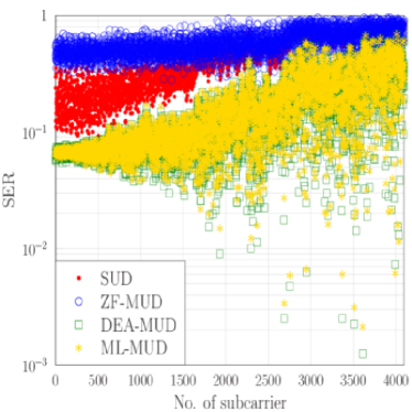
Figure 5: NMSE versus the subcarrier index: (a) $E_{b}/N_{0}=20$ dB, and (b) $E_{b}/N_{0}=30$ dB.

(a)                                                                     (b)

Figure 6: Idealized SER based on perfect CSI versus the subcarrier index: (a) $E_{b}/N_{0}=20$ dB, and (b) $E_{b}/N_{0}=30$ dB.

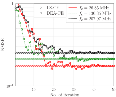
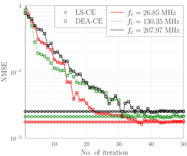
(a)                                                                     (b)

Figure 7: NMSE versus the number of iterations: (a) $E_{b}/N_{0}=20$ dB, and (b) $E_{b}/N_{0}=30$ dB.

V-A Per subcarrier NMSE and SER performance of non-turbo CE and MUD

Let us now consider the non-turbo DEA-CE and DEA-MUD, where the channel estimator relies purely on the pilot symbols only, while the turbo MUD and the decoder perform iterative detection and decoding based on the perfect CSI. This enables us to investigate both the NMSE of the DEA-CE and the ideal symbol error ratio (SER) of the DEA-MUD, separately, on each subcarrier. Note that the interleaving operation makes it impossible for us to investigate the bit error rate (BER) of each individual subcarrier.

The NMSE performance of the DEA-CE at $E_{b}/N_{0}=20$ dB and 30 dB is shown in Fig. 6 (a) and Fig. 6(b), respectively, where $E_{b}$ is the energy per bit and $N_{0}=\sigma_{w}^{2}$ is the noise power. Observe that the DEA-CE achieves an almost identical estimation performance to the LS-CE relying on the same pilot symbols. The idealized SER performance based on the perfect CSI achieved by the DEA-MUD at $E_{b}/N_{0}=20$ dB and 30 dB is depicted in Fig. 6 (a) and Fig. 6 (b), respectively, in comparison to the idealized SERs of the SUD, ZF-MUD and ML-MUD. As expected, the DEA-MUD exhibits a much better detection performance than both the SUD as well as the ZF-MUD, and it is capable of approaching the performance of the ML-MUD. Observe that the detection performance improvement of the DEA-MUD over both the SUD and over the ZF-MUD is more significant at high frequencies. Interestingly, the SUD outperforms the ZF-MUD at low frequencies, because the latter suffers from serious noise enhancement.

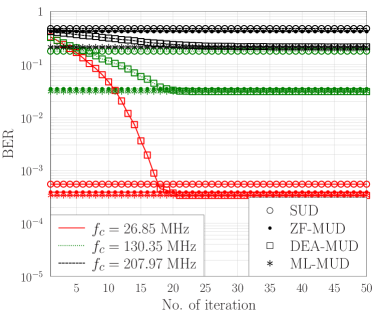
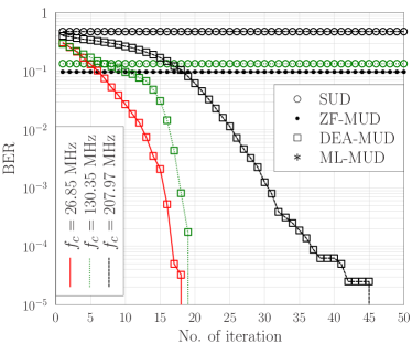
(a)                                                                     (b)

Figure 8: Idealized BER based on perfect CSI versus the number of iterations: (a) $E_{b}/N_{0}=20$ dB, and (b) $E_{b}/N_{0}=30$ dB.

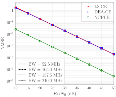
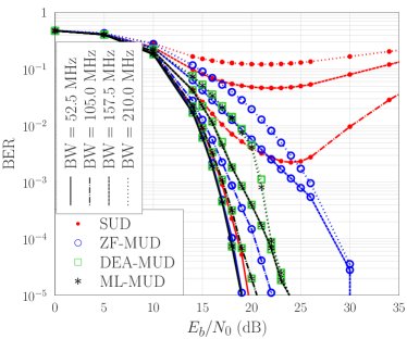
(a)                                                                     (b)

Figure 9: (a) Training-based NMSE performance versus $E_{b}/N_{0}$, and (b) idealized BER performance versus $E_{b}/N_{0}$ relying on perfect CSI, for the system bandwidths of 52.5 MHz, 105.0 MHz, 157.5 MHz and 210.0 MHz.

V-B Convergence of DEA aided CE and DEA aided MUD

By operating the non-turbo DEA aided CE and DEA aided MUD, we can further investigate the convergence of the DEA-CE and the convergence of the DEA-MUD separately. The convergence performance of the DEA-CE and the DEA-MUD are shown in Figs. 7 and 8, respectively, at $E_{b}/N_{0}=20$ dB and 30 dB. Explicitly, we investigate three subcarriers, the 500-th, 2500-th and 4000-th tones having the central frequencies of $f_{c}=26.85$ MHz, 130.35 MHz and 207.97 MHz, respectively, where $f_{c}=26.85$ MHz is in the frequency range of the VDSL2 standard [13], while $f_{c}=130.35$ MHz and 207.97 MHz are in the frequency range of G.fast.

It can be seen from Fig 7 that the DEA-CE converges to the LS-CE solution within 30 iterations at $E_{b}/N_{0}=20$ dB and within 40 iterations at $E_{b}/N_{0}=30$ dB, respectively. At $E_{b}/N_{0}=20$ dB, the BERs of the DEA-MUD converge to those of the ML-MUD around 20 iterations, as seen from Fig. 8 (a). Note that at $E_{b}/N_{0}=30$ dB, the BER of the SUD at $f_{c}=26.85$ MHz, the BERs of the ZF-MUD at $f_{c}=26.85$ MHz and 130.35 MHz as well as the BERs of the ML-MUD at all the three subcarriers are not included in Fig. 8 (b), because they are infinitesimally low based on the perfect CSI. Observe from Fig. 8 (b) that at $E_{b}/N_{0}=30$ dB, the DEA-MUD converges to the ML-MUD after 18 iterations for $f_{c}=26.85$ MHz, 19 iterations for $f_{c}=130.35$ MHz and 45 iterations for $f_{c}=207.97$ MHz, respectively.

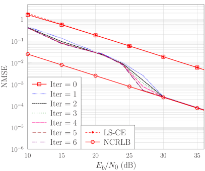
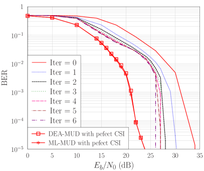
(a)                                                                     (b)

Figure 10: Achievable performance of the DEA aided turbo CE and MUD: (a) NMSE versus $E_{b}/N_{0}$ parametrized by the number of turbo iterations, and (b) BER versus $E_{b}/N_{0}$ parametrized by the number of versus turbo iterations.

V-C Impact of system bandwidth on the achievable performance

As mentioned previously, the channel quality is critically dependent on the system’s bandwidth (BW) or the frequency range. To investigate the influence of the system’s frequency range, we consider four cases: the 1st case at the BW of 52.5 MHz covers the first 1024 subcarriers of the lowest frequency range, the 2nd case covers the first 2048 subcarriers with the BW of 105.0 MHz, the 3rd case has the BW of 157.5 MHz including the first 3072 subcarriers, and the 4th case includes all the 4096 subcarriers and covers the total system BW of 210 MHz.

Fig. 9 (a) depicts the NMSE performance of the DEA-CE based on the pilot symbols. As expected, the NMSE of the DEA-CE is identical to that of the LS-CE, and the system BW has no impact on the training performance of an unbiased channel estimator. Observe from Fig. 9 (a) that there is an approximately 18 dB gap between the training-based NMSE and the NCRLB, where the NCRLB is calculated based on both the pilots and the data. Fig. 9 (b) shows the idealized BER performance of the DEA-MUD based on the perfect CSI for different system bandwidths. As expected, the BER performance is better for the system having a lower frequency range, because the channel quality at a lower frequency range is better. The results of Fig. 9 (b) also confirm that the DEA-MUD and the ML-MUD exhibit almost identical detection performance, and the DEA-MUD outperforms both the SUD and the ZF-MUD, particularly for the systems including higher frequencies. For example, for the system including all the 4096 subcarriers, the DEA-MUD attains an approximately 7 dB SNR gain over the ZF-MUD at the BER level of $10^{-5}$. For this system, the SUD exhibits a high error floor.

V-D Achievable performance of the DEA aided turbo CE and MUD

We now investigate the achievable performance of the proposed DEA aided turbo CE and MUD. Again, we consider the system relying on all the 4096 subcarriers and having the total system bandwidth of 210 MHz. The NMSE and BER versus $E_{b}/N_{0}$ performance of this DE aided turbo CE and MUD scheme is parametrized by the number of turbo iterations, as depicted in Fig. 10 (a) and Fig. 10 (b), respectively.

The results of Fig. 10 need further explanations. Initially, given the training pilots, the DEA-CE estimates the channel, and the NMSE of this channel estimate is given by the $\text{Iter}=0$ curve of Fig. 10 (a), which is identical to that of the training based LS-CE. Given this estimate, the DEA-MUD and the channel decoder perform detection and decoding by iteratively exchanging soft extrinsic information, and after convergence, the detected data exhibits the BER represented by the $\text{Iter}=0$ curve of Fig. 10 (b). The detected data are then fed back to the DEA-CE, which carries out the next CE iteration based on both the detected data and pilots, leading to the improved NMSE as seen from Fig. 10 (a). The enhanced estimated CSI is in turn exploited by the DEA-MUD/channel decoder for producing the detected data at an even lower BER. This ‘turbo’ procedure continues until at the 6th iteration and around the SNR of 27 dB, the BER of the detected data becomes infinitesimally low. Observe from Fig. 10 (a) that at this point, the NMSE of the DEA aided turbo CE and MUD approaches the NCRLB. Explicitly, at the 6th iteration and around the SNR of 27 dB, the achievable NMSE has approached the NCRLB. This is because at this point, the detected data becomes the true data. Not surprisingly, at this point, the BER of the DEA aided turbo CE and MUD approaches that of the idealized ML-MUD associated with perfect CSI, which is also identical to that of the idealized DEA-MUD relying on perfect CSI.

It is worth emphasizing the significance of the iterative gain obtained. Specifically, by iteratively exchanging extrinsic information between the continuous DEA aided CE and the discrete DEA aided MUD, approximately 18 dB of NMSE gain as attained for the channel estimator and around 10 dB of SNR gain is achieved for the MUD.

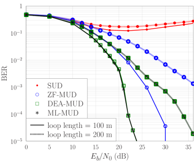
Figure 11: Impact of loop length on the achievable detection performance of four idealized MUDs associated with perfect CSI.

V-E Impact of loop length

Although the lengths of the users’ DSL lines are different in practical deployments, for the convenience of investigating the impact of loop length, we assume that all the users have the same loop length. Fig. 11 shows the influence of the loop length of DSL lines on the achievable BER performance of the four idealized MUDs based on perfect CSI. It can be clearly seen from Fig. 11 that increasing the loop length significantly degrades the achievable BER performance. Observe furthermore from Fig. 11 that the DEA-MUD attains the optimal performance of the ML-MUD, and it considerably outperforms the ZF-MUD. For these two systems, the SUD exhibits high BER floors.

V-F Impact of impulse noise

Next we investigate the impact of impulse noise on the achievable BER performance. When the additive impulse noise is taken into account, the system model (1) can be rewritten as

$$\boldsymbol{Y}= \boldsymbol{H}\boldsymbol{X}+\boldsymbol{W}+\boldsymbol{U},$$ (42)

where $\boldsymbol{U}\in\mathbb{C}^{L}$ is the impulse noise vector. An OFDM symbol is infected by the impulse noise with the probability of $\kappa$, where typically we have $\kappa\in[0.01,~{}0.1]$ [53, 54]. Note that an OFDM symbol includes the data at all the tones, $\boldsymbol{X}[1],\cdots,\boldsymbol{X}[4096]$, where we have re-introduced the omitted tone index of $\boldsymbol{X}$. We assume that the impulse noise $\boldsymbol{U}$ obeys the complex Gaussian distribution associated with a zero-mean vector and the covariance matrix $\sigma^{2}_{u}\boldsymbol{I}_{L}$. Typically, the impulse noise is 20 dB stronger than the additive Gaussian noise $\boldsymbol{W}$ [55, 56], that is, $10\log_{10}\left(\sigma_{u}^{2}/\sigma_{w}^{2}\right)=20$ dB. In our simulations, we consider both $\kappa=0.01$ and $\kappa=0.1$, which can be viewed as the lower bound and the upper bound of the probability that an OFDM symbol is infested by impulse noise.

It can be seen from Fig. 12 that the impulse noise degrades the achievable detection performance, particularly for high $\kappa$, where the case of $\kappa=0$ corresponds to no impulse noise. It can also be seen that at $\kappa=0.01$, both the ML-MUD and the DEA-MUD exhibit almost an identical performance, while at $\kappa=0.1$, the DEA-MUD is slightly inferior to the ML-MUD. Not surprisingly, the DEA-MUD considerably outperforms the ZF-MUD.

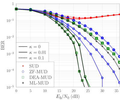
Figure 12: Impact of impulse noise on the achievable detection performance of four idealized MUDs associated with perfect CSI.

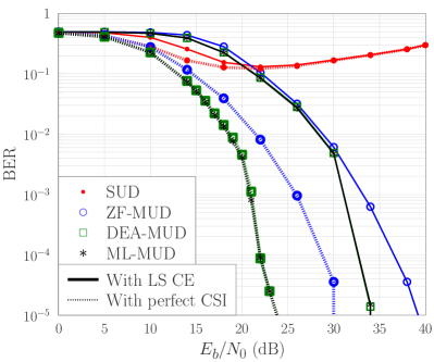
Figure 13: Comparison of the achievable detection performance of four MUDs based on LS-CE acquired by training as well as based on perfect CSI.

V-G Impact of channel estimation error

In Fig. 13, we compare the BER performance of the four MUDs based on the LS-CE acquired by training to those associated with perfect CSI. Clearly, the channel estimation error has a significant impact on the achievable detection performance of an MUD. Explicitly, for both the DEA-MUD and the ML-MUD, there exists an SNR gap of around 10 dB between the idealized performance associated with the perfect CSI and the performance associated with the estimated CSI, which can also be seen from Fig. 10 (b). It can also be seen from Fig. 13, that the SNR gap is approximately 9 dB between the idealized ZF-MUD associated with perfect CSI and the ZF-MUD based estimated CSI.

V-H Computational complexity comparison

As demonstrated by the aforementioned results, given the same CSI, the DEA-MUD is capable of attaining the optimal detection performance of the ML-MUD. We now compare the computational complexity of the DEA-MUD to that of the ML-MUD. Again, the ML-MUD finds the optimal solution by evaluating the CF values of all the $M^{L}=16^{4}=65536$ potential candidates on each single tone. By contrast, the discrete DEA evolves a population of ‘candidates’, as detailed in Section III-C, based on the CF values of the population. Let $N_{\rm ML}$ be the total number of CF evaluations imposed by the ML-MUD and let $N_{\rm DEA}$ be the total number of CF evaluations required by the DEA to converge to the optimal ML solution. We can compare the computational complexities of both the DEA-MUD and of the ML-MUD by calculating the ratio

$$\text{Complexity of DEA-MUD}= \frac{N_{\rm DEA}}{N_{\rm ML}}~{}[\%],$$ (43)

which we use to quantify the computational complexity of the DEA-MUD, in comparison to the ML-MUD.

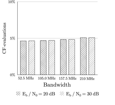
Figure 14: Computational complexity of the DEA-MUD expressed as the ratio of its required CF evaluations over the total CF evaluations imposed by the ML-MUD. The perfect CSI is assumed.

Fig. 14 compares the complexities of the DEA-MUD to those of the ML-MUD for the same four systems as specified in Section LABEL:S4.3 at both $E_{b}/N_{0}=20$ dB and 30 dB. It can be seen from Fig. 14 that the DEA-MUD only requires 5% of the computational complexity imposed by the ML-MUD, while still attaining the same optimal solution as the ML-MUD.

VI Conclusions

We have proposed a DEA aided turbo CE and MUD for mitigating the adverse effects of FEXT encountered by the G.Fast systems caused by the utilization of high frequencies up to 212 MHz. The proposed DEA aided turbo CE and MUD is constituted by a continuous DEA aided CE and a discrete DEA aided MUD, exchanging extrinsic information between them. We have demonstrated that our DEA-MUD significantly outperforms the widely adopted low-complexity ZF-MUD, also known as the ZF-FEXT canceller. More remarkably, we have shown that given the same CSI, our discrete DEA aided MUD is capable of attaining the optimal performance of the ML-MUD, while only imposing 5% of the computational complexity associated with the ML-MUD. In our simulation study, we have also investigated the impact of CE error, of the impulse noise and of the loop length. Most importantly, in this paper, we have demonstrated that by iteratively exchanging information between the continuous DEA aided CE and the discrete DEA aided MUD, the DEA-CE is capable of approaching the optimal CRLB of the channel estimate, while the DEA-MUD based on the estimated CSI is capable of attaining the optimal detection performance of the idealized ML-MUD associated with perfect CSI. Specifically, we have shown that 18 dB of the NMSE gain is attained by the channel estimator and 10 dB of the SNR gain is gleaned by the MUD by exploiting iteration gains. This study therefore has demonstrated that the proposed DEA aided turbo CE and MUD is capable of offering near-capacity performance at an affordable complexity for the emerging G.fast systems.

References

- [1] V. Oksman, et al., “The ITU-T’s new G.fast standard brings DSL into the Gigabit era,” IEEE Commun. Mag., vol. 54, no. 3, pp. 118–126, Mar. 2016.
- [2] F. Effenberger, “Future broadband access networks,” Proc. IEEE, vol. 104, no. 11, pp. 2078–2081, Nov. 2016.
- [3] P. Odling, et al., “The fourth generation broadband concept,” IEEE Commun. Mag., vol. 47, no. 1, pp. 62–69, Jan. 2009.
- [4] I. Binyamini and I. Bergel, “Adaptive precoder using sign error feedback for FEXT cancellation in multichannel downstream VDSL,” IEEE Trans. Signal Process., vol. 61, no. 9, pp. 2383–2393, May 2013.
- [5] G. Ginis and J. M. Cioffi, “Vectored transmission for digital subscriber line systems,” IEEE J. Sel. Areas Commun., vol. 20, no. 5, pp. 1085–1104, Jun. 2002.
- [6] A. Zanko, I. Bergel, and A. Leshem, “Gigabit DSL: a deep-LMS approach,” in Proc. EUSIPCO 2016 (Budapest, Hungary), Aug. 29-Sep. 2, 2016, pp. 300–304.
- [7] ITU-T G.993.5, “Self-FEXT cancellation (vectoring) for use with VDSL2 transceivers,” ITU, 04/2010.
- [8] G. Ginis and J. M. Cioffi, “A multi-user precoding scheme achieving crosstalk cancellation with application to DSL systems,” in Proc. 34th Asilomar Conf. Signals, Systems and Computers (Pacific Grove, CA), Oct. 29-Nov. 1, 2000, pp. 1627–1631.
- [9] M. Hekrdla, et al., “Ordered Tomlinson-Harashima precoding in G.fast downstream,” in Proc. GLOBECOM 2015 (San Diego, CA), Dec. 6-10, 2015, pp. 1–6.
- [10] R. Zhang, A. F. Al Rawi, L. D. Humphrey, and L. Hanzo, “Expanded constellation mapping for enhanced far-end-cross-talk cancellation in G.fast,” IEEE Commun. Let., vol. 21, no. 1, pp. 56–59, Jan. 2017.
- [11] J. Maes, C. Nuzman, and P. Tsiaflakis, “Sensitivity of nonlinear precoding to imperfect channel state information in G.fast,” in Proc. EUSIPcO 2016 (Budapest, Hungary), Aug. 29-Sep. 2, 2016, pp. 290–294.
- [12] R. Cendrillon, G. Ginis, E. Van den Bogaert, and M. Moonen, “A near-optimal linear crosstalk canceler for upstream VDSL,” IEEE Trans. Signal Process., vol. 54, no. 8, pp. 3136–3146, Aug. 2006.
- [13] P.-E. Eriksson and B. Odenhammar, “VDSL2: next important broadband technology,” Ericsson Review, vol. 1, pp. 36–47, 2006.
- [14] S. M. Zafaruddin, S. Prakriya, and S. Prasad, “Performance of linear minimum-output energy receiver for self and alien crosstalk mitigation in upstream vectored very high-speed digital subscriber line,” IET Commun., vol. 9, no. 6, pp. 862–871, Apr. 2015.
- [15] A. Leshem and Y. Li, “A low complexity linear precoding technique for next generation VDSL downstream transmission over copper,” IEEE Trans. Signal Process., vol. 55, no. 11, pp. 5527–5534, Nov. 2007.
- [16] J. Louveaux and A.-J. Van Der Veen, “Error sign feedback as an alternative to pilots for the tracking of FEXT transfer functions in downstream VDSL,” EURASIP J. Applied Signal Process., vol. 2006, pp. 1–14, Jan. 2006.
- [17] ——, “Adaptive DSL crosstalk precancellation design using low-rate feedback from end users,” IEEE Signal Process. Let., vol. 13, no. 11, pp. 665–668, Nov. 2006.
- [18] ——, “Adaptive precoding for downstream crosstalk precancelation in DSL systems using sign-error feedback,” IEEE Trans. Signal Process., vol. 58, no. 6, pp. 3173–3179, Jun. 2010.
- [19] W. Lanneer, P. Tsiaflakis, J. Maes, and M. Moonen, “Linear and nonlinear precoding based dynamic spectrum management for downstream vectored G.fast transmission,” IEEE Trans. Commun., vol. 65, no. 3, pp. 1247–1259, Mar. 2017.
- [20] A. H. Fazlollahi, X. Wang, and Y. Zeng, “FEXT Exploitation in next generation DSL systems,” in Proc. GLOBECOM 2016 (Washington, DC, USA), Dec.4-8, 2016, pp. 1–6.
- [21] W. Yao, S. Chen, and L. Hanzo,, “A transceiver design based on uniform channel decomposition and MBER vector perturbation,” IEEE Trans. Vehicular Tech., vol. 59, no. 6, pp. 3153–3159, Jul. 2010.
- [22] ——, “Generalised MBER-based vector precoding design for multiuser transmission,” IEEE Trans. Vehicular Tech., vol. 60, no. 2, pp. 739–745, Feb. 2011.
- [23] K.-W. Cheong, W.-J. Choi, and J. M. Cioffi, “Multiuser soft interference canceler via iterative decoding for DSL applications,” IEEE J. Sel. Areas Commun., vol. 20, no. 2, pp. 363–371, Feb. 2002.
- [24] G.-H. Im, K.-M. Kang, and C.-J. Park, “FEXT cancellation for twisted-pair transmission,” IEEE J. Sel. Areas Commun., vol. 20, no. 5, pp. 959–973, Jun. 2002.
- [25] R. Hormis, D. Guo, and X. Wang, “Monte Carlo FEXT cancellers for DSL channels,” IEEE Trans. Circuits and Systems I, vol. 52, no. 9, pp. 1894–1908, Sep. 2005.
- [26] J. M. Cioffi and G. Forney Jr, “Generalized decision-feedback equalization for packet transmission with ISI and Gaussian noise,” in A. Paulraj, V. Roychowdhury, and C. D. Schaper (eds.), Communications, Computation, Control, and Signal Processing, Springer: NY, 1997, pp. 79–127.
- [27] C.-Y. Chen, K. Seong, R. Zhang, and J. M. Cioffi, “Optimized resource allocation for upstream vectored DSL systems with zero-forcing generalized decision feedback equalizer,” IEEE J. Sel. Topics Signal Process., vol. 1, no. 4, pp. 686–699, Dec. 2007.
- [28] P. Biyani, et al., “Co-operative alien noise cancellation in upstream VDSL: a new decision directed approach,” IEEE Trans. Commun., vol. 61, no. 8, pp. 3494–3504, Aug. 2013.
- [29] W. Yao, S. Chen, S. Tan, and L. Hanzo, “Minimum bit error rate multiuser transmission designs using particle swarm optimisation,” IEEE Trans. Wireless Commun., vol. 8, no. 10, pp. 5012–5017, Oct. 2009.
- [30] W. Yao, S. Chen, and L. Hanzo, “Particle swarm optimisation aided multiuser transmission schemes for MIMO communication,” in Proc. 3rd Int. Conf. Bio-Inspired Systems and Signal Process. (Valencia, Spain), Jan.20-23, 2010, pp. 53–60.
- [31] ——, “Particle swarm optimisation aided MIMO multiuser transmission designs,” J. Computational and Theoretical Nanoscience, vol. 9, no.2, pp. 266–275, Feb. 2012.
- [32] K. Yen and L. Hanzo, “Genetic algorithm assisted joint multiuser symbol detection and fading channel estimation for synchronous CDMA systems,” IEEE J. Sel. Areas Commun., vol. 19, no. 6, pp. 985–998, Jun. 2001.
- [33] H. R. Palally, S. Chen, W. Yao, and L. Hanzo,“Particle swarm optimisation aided semi-blind joint maximum likelihood channel estimation and data detection for MIMO systems,” in Proc. SSP09 (Cardiff, UK), Aug. 31-Sep., 2009, pp. 309–312.
- [34] J. Zhang, S. Chen, X. Mu, and L. Hanzo, “Joint channel estimation and multi-user detection for SDMA/OFDM based on dual repeated weighted boosting search,” IEEE Trans. Vehicular Tech., vol. 60, no 7, pp. 3265–3275, Sep. 2011.
- [35] ——, “Differential evolution algorithm aided minimum symbol error rate multi-user detection for multi-user OFDM/SDMA systems,” in Proc. VTC 2012 Spring (Yokohama, Japan), May 6-9, 2012, pp. 1–5.
- [36] ——, “Turbo multi-user detection for OFDM/SDMA systems relying on differential evolution aided iterative channel estimation,” IEEE Trans, Commun., vol. 60, no. 6, pp. 1621–1663, Jun. 2012.
- [37] ——, “Benchmarking capabilities of evolutionary algorithms in joint channel estimation and turbo multi-user detection/decoding,” in Proc. CEC 2013 (Cancun, Mexico), Jun. 20-23, 2013, pp. 3354–3362.
- [38] ——, “Evolutionary-algorithm-assisted joint channel estimation and turbo multiuser detection/decoding for OFDM/SDMA,” IEEE Trans. Vehicular Tech., vol. 63, no. 3, pp. 1204–1222, Mar. 2014.
- [39] K. Price, R. M. Storn, and J. A. Lampinen, Differential Evolution: A Practical Approach to Global Optimization. Berlin: Springer Verlag, 2005.
- [40] A. Qin, V. L. Huang, and P. N. Suganthan, “Differential evolution algorithm with strategy adaptation for global numerical optimization,” IEEE Trans. Evolutionary Computation, vol. 13, no. 2, pp. 398–417, Apr. 2009.
- [41] L. Hanzo, O. R. Alamri, M. El-Hajjar, and N. Wu, Near-Capacity Multi-Functional MIMO Systems: Sphere-Packing, Iterative Detection and Cooperation. Chichester, UK: Wiley, 2009.
- [42] S. Tan, S. Chen, and L. Hanzo, “On multi-user EXIT chart analysis aided turbo-detected MBER beamforming designs,” IEEE Trans. Wireless Commun., vol. 7, no. 1, pp. 314–323, Jan. 2008.
- [43] L. Xu, S. Chen, and L. Hanzo, “EXIT chart analysis aided turbo MUD designs for the rank-deficient multiple antenna assisted OFDM uplink,” IEEE Trans. Wireless Commun., vol. 7, no. 6, pp. 2039–2044, Jun. 2008.
- [44] R. Zhang, L. Xu, S. Chen, and L. Hanzo, “EXIT-chart-aided hybrid multiuser detector for multicarrier interleave-division multiple access,” IIEEE Trans. Vehicular Tech., vol. 59, no. 3, pp. 1563–1567, Mar. 2010.
- [45] S. Sugiura, S. Chen, and L. Hanzo, “MIMO-aided near-capacity turbo transceivers: taxonomy and performance versus complexity,” IEEE Commun. Surveys and Tutorials, vol. 14, no.2, pp. 421–442, 2012.
- [46] P. Zhang, S. Chen, and L. Hanzo, “Reduced-complexity near-capacity joint channel estimation and three-stage turbo detection for coherent space-time shift keying,” IEEE Trans. Commun., vol. 61, no. 5, pp. 1902–1913, May 2013.
- [47] ——, “Embedded iterative semi-blind channel estimation for three-stage-concatenated MIMO-aided QAM turbo-transceivers,” IEEE Trans. Vehicular Tech., vol. 63, no. 1, pp. 439–446, Jan. 2014.
- [48] ——, “Two-tier channel estimation aided near-capcity MIMO transceivers relaying on norm-based joint transmit and receive antenna selection,” IEEE Trans. Wireless Commun., vol. 14, no. 1, pp. 122–137, Jan. 2015.
- [49] Q. Wang, et al., “A universal low-complexity symbol-to-bit soft demapper,” IEEE Trans. Vehicular Tech., vol. 63, no. 1, pp. 119–130, Jan. 2014.
- [50] N. L. Johnson, S. Kotz, and N. Balakrishnan, Continuous Univariate Distributions. New York: Wiley, 1994.
- [51] J. Havil, Gamma: Exploring Euler’s Constant. Princeton, NJ: Princeton University Press, 2003.
- [52] S. M. Kay, Fundamentals of Statistical Signal Processing: Estimation Theory. Englewood Cliffs, NJ: Prentice-Hall, 1993.
- [53] R. Kirkby, “Realistic impulsive noise model,” ETSI TM6 011T20, 2001.
- [54] G. Ndo, F. Labeau, and M. Kassouf, “A Markov-Middleton model for bursty impulsive noise: Modeling and receiver design,” IEEE Trans. Power Delivery, vol. 28, no. 4, pp. 2317–2325, Oct. 2013.
- [55] J. Neckebroek, M. Moeneclaey, M. Guenach, M. Timmers, and J. Maes, “Comparison of error-control schemes for high-rate communication over short DSL loops affected by impulsive noise,” in Proc. ICC 2013 (Budapest, Hungary), Jun. 9-13, 2013, pp. 4014–4019.
- [56] T. Bai, et al., “Discrete multi-tone digital subscriber loop performance in the face of impulsive noise,” IEEE Access, vol. 5, pp. 10478–10495, Jun. 2017.