Accelerating delayed-acceptance Markov chain Monte Carlo algorithms

Abstract

Delayed-acceptance Markov chain Monte Carlo (DA-MCMC) samples from a probability distribution via a two-stages version of the Metropolis-Hastings algorithm, by combining the target distribution with a “surrogate” (i.e. an approximate and computationally cheaper version) of said distribution. DA-MCMC accelerates MCMC sampling in complex applications, while still targeting the exact distribution. We design a computationally faster, albeit approximate, DA-MCMC algorithm. We consider parameter inference in a Bayesian setting where a surrogate likelihood function is introduced in the delayed-acceptance scheme. When the evaluation of the likelihood function is computationally intensive, our scheme produces a 2-4 times speed-up, compared to standard DA-MCMC. However, the acceleration is highly problem dependent. Inference results for the standard delayed-acceptance algorithm and our approximated version are similar, indicating that our algorithm can return reliable Bayesian inference. As a computationally intensive case study, we introduce a novel stochastic differential equation model for protein folding data.

Keywords: Bayesian inference, Gaussian process, pseudo marginal MCMC, protein folding, stochastic differential equation

1 Introduction

We introduce a new strategy to accelerate Markov chain Monte Carlo (MCMC) sampling when the evaluation of the target distribution is computationally expensive. We build on the “delayed-acceptance” (DA) strategy developed in Christen and Fox (2005) where a fast, “two-stages” DA-MCMC algorithm is proposed while still targeting the desired distribution exactly. We produce an approximated and accelerated delayed-acceptance MCMC algorithm (ADA-MCMC), where in exchange of exactness we obtain results even more rapidly than the standard DA-MCMC. In a computationally intensive case study, the run-time for ADA-MCMC is 2–4 times faster than for standard DA-MCMC.

The methodology we consider is general, as our novel method pertains sampling from arbitrary distributions. However, in the interest of our applications, we will focus on Bayesian inference, and then suggest how to implement our ideas for general problems. In Bayesian inference we aim at sampling from the posterior distribution $p(\theta|y)\propto p(y|\theta)p(\theta)$, where $\theta$ are model parameters, $y$ denotes data, $p(y|\theta)$ is the likelihood function, and $p(\theta)$ is the prior distribution of $\theta$. We assume that the point-wise evaluation of the likelihood $p(y|\theta)$ (or an approximation thereof) is computationally intensive, because the underlying probabilistic model is complex and/or the data $y$ is large. For those situations, DA-MCMC algorithms turn particularly useful. In the approach originally outlined in Christen and Fox (2005) a DA strategy decomposes an MCMC move into two stages. At the first stage a proposal can either be rejected, according to a “surrogate of the posterior” (one that is computationally cheap to evaluate and chosen to approximate the desired posterior), or be sent to the second stage. If the proposal is not rejected at the first stage, at the second stage an acceptance probability is used that corrects for the discrepancy between the approximate surrogate and the desired posterior, and at this stage the proposal can finally be accepted or rejected. The advantage of using DA-MCMC is that the computationally expensive posterior only appears in the second stage, whereas the surrogate posterior in the first stage is cheap to evaluate. Therefore, in the first stage the surrogate posterior rapidly screens proposals, and rejects those that are unlikely to be accepted at the second stage, if the surrogate model is reliable. When considering a Bayesian approach, we build a surrogate of the computationally expensive likelihood function, while we assume the cost of evaluating the prior to be negligible. Therefore the expensive likelihood appears only in the second stage. Some implementations of the DA approach in Bayesian inference can be found e.g. in Golightly et al. (2015), Sherlock et al. (2017), and Banterle et al. (2015), and similar approaches based on approximate Bayesian computation (ABC) can be found in Picchini (2014), Picchini and Forman (2016), and Everitt and Rowińska (2017).

In this work, the sequence of computations pertaining the second stage of DA-MCMC are arranged so to find further opportunities to avoid the evaluation of the expensive likelihood. This leads to our accelerated and approximated ADA-MCMC. The computational benefit of using ADA-MCMC is that, unlike DA-MCMC, once a parameter proposal reaches the second stage, the expensive likelihood is not necessarily evaluated, but this comes at the price of introducing an approximation in the sampling procedure. We test and compare delayed-acceptance algorithms, particle marginal methods for exact Bayesian inference, and Markov-chain-within-Metropolis on two case studies: The stochastic Ricker model, and a novel state-space model for protein folding data, with dynamics expressed via a stochastic differential equation (SDE). Therefore, in this work we contribute with: (i) a novel, approximate and accelerated delayed-acceptance MCMC algorithm, and (ii) a novel double-well potential state-space model for protein folding data. For practical applications, we use Gaussian processes to specify surrogates of the likelihood function, though this is not an essential component of our approach and other surrogates of the likelihood can be considered. We found that the acceleration produced by ADA-MCMC, compared to DA-MCMC, is dependent on the specific application. If the exact or approximate likelihood function used in the second stage of the algorithm is not computationally intensive to evaluate, then our method produces negligible benefits. Therefore, the use of our ADA-MCMC, just as the standard DA-MCMC, is beneficial when each evaluation of the likelihood has a non-negligible impact on the total computational budget. Then, the time savings due to ADA-MCMC are proportional to the number of MCMC iterations where the evaluation of the likelihood at the second stage is avoided. In terms of inference quality, we find that ADA-MCMC returns results that are very close to DA-MCMC, so our approximations do not seem to harm the accuracy of the resulting inference.

The outline of this paper is as follows: The delayed-acceptance (DA) scheme and our novel accelerated DA algorithm are introduced in a general framework in Section 2. The Gaussian process (GP) surrogate model is introduced in Section 3. The DA-GP-MCMC algorithm and the accelerated version ADA-GPMCMC are introduced in Section 4. A simulation study for the stochastic Ricker model is in Section 5.1. The protein folding data and the novel double-well potential stochastic differential equation model are introduced in Section 5.2. A discussion in Section 6 closes our work. Further supplementary material is available, outlining: particle Markov chain Monte Carlo methods for state-space models, implementation guidelines for the algorithms, a further simulation study, and diagnostic analyses. The code used to generate results can be found at https://github.com/SamuelWiqvist/adamcmcpaper and in the supplementary material.

2 Delayed-acceptance MCMC

We first introduce the delayed-acceptance (DA-MCMC) scheme due to Christen and Fox (2005) in full generality, then we specialize it for Bayesian inference. Our accelerated delayed-acceptance (ADA-MCMC) algorithm is introduced in section 2.1. We are interested in sampling from some distribution $p(x)$ using Metropolis-Hastings (Hastings, 1970). Metropolis-Hastings proceeds by evaluating random moves produced by a Markov kernel from the current value of $x$ to a new $x^{\star}$. The sequence of accepted moves forms a Markov chain having $p(x)$ as stationary distribution. Now, assume that the point-wise evaluation of $p(x)$ is computationally expensive. The main idea behind a DA-MCMC approach is to delay (or avoid as much as possible) the evaluation of the computationally expensive $p(x)$, by first trying to early-reject the proposal $x^{\star}$ using some surrogate (cheap to evaluate) deterministic or stochastic model $\tilde{p}(x)$. To enable early-rejections while still targeting the distribution $p(x)$, a two-stages acceptance scheme is introduced in Christen and Fox (2005). Say that we are at the $r$th iteration of the Metropolis-Hastings algorithm, and denote with $x^{r-1}$ the state of the chain produced at the previous iteration. At the “first stage” of DA-MCMC we evaluate the acceptance probability (though at this stage we do not really accept any proposal as explained below)

$$\alpha_{1}=\min\biggl{(}1,\frac{\tilde{p}(x^{\star})}{\tilde{p}(x^{r-1})}\cdot\frac{g(x^{r-1}|x^{\star})}{g(x^{\star}|x^{r-1})}\biggr{)},$$ (1)

where $g(x|y)$ is the transition kernel used to generate proposals, i.e. at the $r$th iteration $x^{\star}\sim g(x|x^{r-1})$. If the proposal $x^{\star}$ “survives” the first stage (i.e. if it is not rejected) it is then promoted to the second stage where it is accepted with probability $\alpha_{2}$,

$$\alpha_{2}=\min\biggl{(}1,\frac{p(x^{\star})}{p(x^{r-1})}\cdot\frac{\tilde{p}(x^{r-1})}{{\tilde{p}}(x^{\star})}\biggr{)}.$$ (2)

Therefore $x^{\star}$ can only be accepted at the second stage, while it can be rejected both at the first and second stage. A computational speed-up is obtained when $x^{\star}$ is early-rejected at the first stage, as there the expensive $p(x^{\star})$ is not evaluated. Hence, to obtain a significant speed-up it is important to early-reject “bad” proposals that would likely be rejected at the second stage. The probability $\alpha_{2}$ corrects for the approximation introduced in the first stage and the resulting Markov chain has the correct stationary distribution $p(x)$. This result holds if $g$ is $p$-irreducible and reversible, and if $g(x|y)>0$ implies $\tilde{p}(x)>0$. From (2) it is evident how the surrogate model acts as a proposal distribution. See Franks and Vihola (2017) for a comparison in terms of asymptotic variances of Monte Carlo estimators provided via importance sampling, pseudo-marginal and delayed-acceptance methods.

In a Bayesian framework we are interested in sampling from the posterior $p(\theta|y)\propto p(y|\theta)p(\theta)$. Furthermore, for the cases of interest to us, the log-likelihood function (or an approximation thereof) $\ell(\theta):=\log p(y|\theta)$, is computationally expensive while the prior distribution is assumed cheap to evaluate. By introducing a deterministic or stochastic surrogate likelihood $\tilde{L}(\theta):=\exp(\tilde{\ell}(\theta))$, DA has first stage acceptance probability $\alpha_{1}$, where

$$\alpha_{1}=\min\biggl{(}1,\frac{\tilde{L}(\theta^{\star})}{\tilde{L}(\theta^{r-1})}\cdot\frac{p(\theta^{\star})}{p(\theta^{r-1})}\cdot\frac{g(\theta^{r-1}|\theta^{\star})}{g(\theta^{\star}|\theta^{r-1})}\biggr{)},$$

with transition kernel $g$. Similarly, by setting ${L}(\theta):=\exp({\ell}(\theta))$, the second stage acceptance probability is

$$\alpha_{2}=\min\biggl{(}1,\frac{L(\theta^{\star})}{L(\theta^{r-1})}\cdot\frac{\tilde{L}(\theta^{r-1})}{\tilde{L}(\theta^{\star})}\biggr{)}.$$

An extension of the DA-MCMC scheme due to Sherlock et al. (2017) is to generate a proposal $\theta^{\star}$ from a different transition kernel $\tilde{g}(\cdot|\theta^{r-1})$, and with a small but positive probability $\beta_{MH}\in(0,1)$ allow the evaluation of the proposal $\theta^{\star}$ in an ordinary Metropolis-Hastings algorithm, with acceptance probability denoted $\alpha_{MH}$,

$$\alpha_{MH}=\min\biggl{(}1,\frac{L(\theta^{\star})}{L(\theta^{r-1})}\cdot\frac{p(\theta^{\star})}{p(\theta^{r-1})}\cdot\frac{\tilde{g}(\theta^{r-1}|\theta^{\star})}{\tilde{g}(\theta^{\star}|\theta^{r-1})}\biggr{)}.$$ (3)

In this case the proposal can be immediately accepted or rejected as in a regular MCMC. The transition kernel $g$ should have a somewhat larger variance than $\tilde{g}$. With probability $1-\beta_{MH}$ a proposal is instead evaluated using the two-stages DA-MCMC algorithm. When considering this “extended version” of DA-MCMC (where $\beta_{MH}$ is introduced) it is preferable to use a small $\beta_{MH}$ in order not to lose too much of the acceleration implied by a DA approach. Our experience also indicates that this extension can be critical to better explore the tails of the posterior distribution, compared to a standard DA-MCMC that uses $\beta_{MH}=0$. This "mixture" of the two Metropolis-Hastings kernels (i.e. the acceptance kernel for the DA scheme, and the acceptance kernel in (3)) produces a valid MCMC algorithm, since both kernels in the standard cases target the correct posterior (Rosenthal and Roberts, 2007).

2.1 Accelerated delayed-acceptance MCMC

There have been a number of attempts at accelerating the original DA-MCMC of Christen and Fox (2005). For example, in a Bayesian framework, Banterle et al. (2015) propose to break down the posterior into the product of $d$ chunks. The Metropolis-Hastings acceptance ratio becomes the product of $d$ acceptance ratios, each of which can be sequentially evaluated against one of $d$ independent uniform variates. The acceleration is given by the possibility to “early-reject” a proposal, as soon as one of those acceptance ratios leads to a rejection (in the same spirit of Solonen et al., 2012). However, an acceptance requires instead the scanning of all $d$ components, i.e. the full posterior. Quiroz et al. (2017) never use the full data set in the second stage of DA and instead construct an approximated likelihood from subsamples of the data, which is particularly relevant for Big Data problems (see references therein and Angelino et al., 2016). Remarkably, Quiroz et al. (2017) prove that even when the full likelihood is approximated using data subsamples, the resulting chain has the correct stationary distribution. However, they assume data to be conditionally independent, a strong condition which does not apply to case studies considered in the present work.

We now introduce the novel, accelerated DA-MCMC algorithm, shortly ADA-MCMC. The main idea behind ADA-MCMC is that, under some assumptions on how the likelihood function and the surrogate model relate, it is possible to arrange the computations in the second stage to obtain an acceleration in the computations. This is implied by the possibility to avoid the evaluation of the expensive likelihood in the second stage, in some specific circumstances. However, this also implies that ADA-MCMC is an approximated procedure, since a proposal can sometimes be accepted according to the surrogate model. We introduce ADA-MCMC in a Bayesian setting where the surrogate model pertains the likelihood function. However, the idea can straightforwardly be adapted to the case where a surrogate model of a generic distribution $p(x)$ is used, as in Equations (1)-(2). The more general setting is briefly described later in this section. As previously mentioned, at the $r$th iteration the DA algorithm is governed by the values of the likelihood function $L(\theta^{\star})$ and $L(\theta^{r-1})$, and the values of the surrogate model $\tilde{L}(\theta^{\star})$ and $\tilde{L}(\theta^{r-1})$. These four values can be considered arranged in four mutually exclusive scenarios:

$$\text{case 1)}\,\,\tilde{L}(\theta^{\star})>\tilde{L}(\theta^{r-1})\,\,\textit{and}\,\,L(\theta^{\star})>L(\theta^{r-1}),$$

$$\text{case 2)}\,\,\tilde{L}(\theta^{\star})<\tilde{L}(\theta^{r-1})\,\,\textit{and}\,\,L(\theta^{\star})<L(\theta^{r-1}),$$

$$\text{case 3)}\,\,\tilde{L}(\theta^{\star})>\tilde{L}(\theta^{r-1})\,\,\textit{and}\,\,L(\theta^{\star})<L(\theta^{r-1}),$$

$$\text{case 4)}\,\,\tilde{L}(\theta^{\star})<\tilde{L}(\theta^{r-1})\,\,\textit{and}\,\,L(\theta^{\star})>L(\theta^{r-1}).$$

We study each case separately to investigate any opportunity for accelerating the computations in the second stage of DA-MCMC, under the assumption that the relations between the evaluations of $\tilde{L}$ and $L$ hold. Afterwards, we suggest ways to determine approximately which of the four possibilities we should assume to hold, for any new proposal $\theta^{\star}$, without evaluating the expensive likelihood $L(\theta^{\star})$.

Case 1)

Under the assumption that $\tilde{L}(\theta^{\star})>\tilde{L}(\theta^{r-1})$ and $L(\theta^{\star})>L(\theta^{r-1})$ it is clear that $\frac{\tilde{L}(\theta^{r-1})}{\tilde{L}(\theta^{\star})}<1$ and $\frac{L(\theta^{r-1})}{L(\theta^{\star})}<1$. It also holds that

$$\frac{\tilde{L}(\theta^{r-1})}{\tilde{L}(\theta^{\star})}<\frac{L(\theta^{\star})}{L(\theta^{r-1})}\cdot\frac{\tilde{L}(\theta^{r-1})}{\tilde{L}(\theta^{\star})}.$$ (4)

Hence, the acceptance region for the second stage can be split in two parts, where one part is “governed” by $\frac{\tilde{L}(\theta^{r-1})}{\tilde{L}(\theta^{\star})}$ only. To clarify, at the second stage of the standard DA-MCMC, acceptance of a proposed $\theta^{\star}$ takes place if $u<\frac{L(\theta^{\star})}{L(\theta^{r-1})}\cdot\frac{\tilde{L}(\theta^{r-1})}{\tilde{L}(\theta^{\star})}$ where $u\sim U(0,1)$ is uniformly distributed in [0,1], hence, the acceptance region is $\bigl{[}0,\frac{L(\theta^{\star})}{L(\theta^{r-1})}\cdot\frac{\tilde{L}(\theta^{r-1})}{\tilde{L}(\theta^{\star})}\bigr{]}$. However, because of (4) we are allowed to further decompose the acceptance region, as presented below:

Hence, if a proposal $\theta^{\star}$ has survived the first stage and we assume that we are in case 1, we can first check whether we can “early-accept” the proposal (i.e. without evaluating the expensive likelihood), that is, check if

$$u<\frac{\tilde{L}(\theta^{r-1})}{\tilde{L}(\theta^{\star})},$$ (5)

and if this is the case $\theta^{\star}$ is (early)-accepted and stored, and we can move to the next iteration of ADA-MCMC. If $\theta^{\star}$ is not early-accepted, we can look into the remaining part of the [0,1] segment to determine if the proposal can be accepted or rejected. Hence, when early-acceptance is denied, the expensive likelihood $L(\theta^{\star})$ is evaluated and the proposal is accepted and stored if

$$u<\frac{L(\theta^{\star})}{L(\theta^{r-1})}\cdot\frac{\tilde{L}(\theta^{r-1})}{\tilde{L}(\theta^{\star})},$$ (6)

and rejected otherwise, and we can move to the next iteration of ADA-MCMC. Since the acceptance region for the second stage is split in two parts (early-acceptance and acceptance), the same random number $u$ is used in (5) and (6). By splitting the region it is possible to early-accept proposals without evaluating $L(\theta^{\star})$, and thereby obtaining a speed-up.

Case 2)

If this case holds, then $\frac{\tilde{L}(\theta^{r-1})}{\tilde{L}(\theta^{\star})}>1$ and $\frac{L(\theta^{\star})}{L(\theta^{r-1})}<1$. Hence, it is not possible to obtain any early-accept or early-reject opportunity in this case.

Case 3)

If this case holds, then $\frac{\tilde{L}(\theta^{r-1})}{\tilde{L}(\theta^{\star})}<1$ and $\frac{L(\theta^{\star})}{L(\theta^{r-1})}<1$. Hence, it also holds that

$$\frac{\tilde{L}(\theta^{r-1})}{\tilde{L}(\theta^{\star})}>\frac{L(\theta^{\star})}{L(\theta^{r-1})}\cdot\frac{\tilde{L}(\theta^{r-1})}{\tilde{L}(\theta^{\star})}.$$

The rejection region is $\bigl{[}\frac{L(\theta^{\star})}{L(\theta^{r-1})}\cdot\frac{\tilde{L}(\theta^{r-1})}{\tilde{L}(\theta^{\star})},1\bigr{]}$ and this can be split in two parts, where one part is only governed by $\frac{\tilde{L}(\theta^{r-1})}{\tilde{L}(\theta^{\star})}$, see below:

By simulating a $u\sim U(0,1)$, we can first check if the proposal can be early-rejected. This happens if $u>\frac{\tilde{L}(\theta^{r-1})}{\tilde{L}(\theta^{\star})}$. If the proposal is not early-rejected, it is accepted if

$$u<\frac{L(\theta^{\star})}{L(\theta^{r-1})}\cdot\frac{\tilde{L}(\theta^{r-1})}{\tilde{L}(\theta^{\star})},$$

and rejected otherwise. Hence, in case 3 there is a chance to early-reject $\theta^{\star}$ without evaluating $L(\theta^{\star})$.

Case 4)

Under the assumption we have that $\frac{\tilde{L}(\theta^{r-1})}{\tilde{L}(\theta^{\star})}>1$ and $\frac{L(\theta^{\star})}{L(\theta^{r-1})}>1$, and we can immediately accept the proposal without evaluating $L(\theta^{\star})$, since $\frac{L(\theta^{\star})}{L(\theta^{r-1})}\cdot\frac{\tilde{L}(\theta^{r-1})}{\tilde{L}(\theta^{\star})}>1$.

Clearly, assuming a specific case to be the “right one”, for proposal $\theta^{\star}$, is a decision subject to probabilistic error. This is why ADA-MCMC is an approximate version of DA-MCMC. Of course, the crucial problem is to determine which of the four cases to assume to hold for the proposed $\theta^{\star}$. One method is to consider a pre-run of some MCMC algorithm, to estimate the probability $p_{j}$ for each of the four different cases, where $p_{j}$ is the true but unknown probability that case $j$ holds, $j=1,...,4$. This is of course a possibly computationally heavy procedure, however, for the specific algorithms we study in Section 4, such a pre-run is necessary to construct the surrogate model for the log-likelihood, hence the estimation of the $p_{j}$ comes as a simple by-product of the inference procedure. Then, once the estimates $\hat{p}_{j}$ are obtained, for a new $\theta^{\star}$ one first checks if $\frac{\tilde{L}(\theta^{r-1})}{\tilde{L}(\theta^{\star})}<1$ or if $\frac{\tilde{L}(\theta^{r-1})}{\tilde{L}(\theta^{\star})}>1$. If $\frac{\tilde{L}(\theta^{r-1})}{\tilde{L}(\theta^{\star})}>1$ then we can either be in case 2 or 4. We toss a uniform $u$ and if $u<\hat{p}_{2}$ case 2 is selected with probability $\hat{p}_{2}$ (and otherwise case 4 is selected, since $\hat{p}_{4}=1-\hat{p}_{2}$). Correspondingly, if $\frac{\tilde{L}(\theta^{r-1})}{\tilde{L}(\theta^{\star})}<1$ then we can be either in case 1 or 3. We toss a uniform $u\sim U(0,1)$, and if $u<\hat{p}_{1}$ case 1 is selected (otherwise case 3 is selected, since $\hat{p}_{3}=1-\hat{p}_{1}$). Another approach is to model the probabilities as a function of $\theta$. Hence, we are then interested in computing the probabilities $\hat{p}_{1}(\theta)$, $\hat{p}_{2}(\theta)$,$\hat{p}_{3}(\theta)$, and $\hat{p}_{4}(\theta)$. For this task, we can for instance use logistic regression, or some other classification algorithm. The problem of the selection of cases 1–4 is discussed in detail in Section 4.1.

We stated early that ADA can also be used in a non-Bayesian setting, where we target a generic distribution $p(x)$ for some $x\in\mathcal{X}$. In that case we need to introduce a corresponding surrogate model $\tilde{p}(x)$. The $r$th iteration of ADA will then be governed by the four values $\tilde{p}(x^{\star})$, $\tilde{p}(x^{r-1})$, $p(x^{\star})$, and $p(x^{r-1})$, where $x^{\star}$ is a proposed value $x^{*}\in\mathcal{X}$. These can be arranged into four cases, similarly to what previously described: case 1) $\tilde{p}(x^{\star})$ > $\tilde{p}(x^{r-1})$ and $p(x^{\star})$ > $p(x^{r-1})$, 2) $\tilde{p}(x^{\star})$ < $\tilde{p}(x^{r-1})$ and $p(x^{\star})$ < $p(x^{r-1})$, 3) $\tilde{p}(x^{\star})$ > $\tilde{p}(x^{r-1})$ and $p(x^{\star})$ < $p(x^{r-1})$, and 4) $\tilde{p}(x^{\star})$ < $\tilde{p}(x^{r-1})$ and $p(x^{\star})$ > $p(x^{r-1})$. Therefore, by adapting the methodology, possibilities for early-rejection and early-acceptance of a proposal $x^{\star}$ can straightforwardly be obtained regardless of whether we pursue a Bayesian analysis or not.

3 Modeling the log-likelihood function using Gaussian processes

We have outlined our methodology without reference to a specific choice for the surrogate likelihood. A possibility is to use Gaussian process regression to obtain a surrogate log-likelihood $\log\tilde{L}$. Gaussian processes (GPs) is a class of statistical models that can be used to describe the uncertainty about an unknown function. In our case, the unknown function is the log-likelihood $\ell(\theta)=\log p(y|\theta)$. A GP has the property that the joint distribution for the values of the unknown function, at a finite collection of points, has a multivariate normal distribution. As such, each Gaussian process is fully specified by a mean function $m$, and a covariance function $k$ (Rasmussen and Williams, 2006). We introduce a GP regression model, similar to the one used in Drovandi et al. (2018), as a computationally cheap proxy to the unknown log-likelihood $\ell(\theta)$. Our GP model uses covariates that are powers and interactions of the $d$ parameters of interest $\theta=(\theta_{1},...,\theta_{d})$ (see the supplementary material). The GP model assumes

$$\ell(\theta)\sim\mathcal{GP}(m_{\beta}(\theta),k_{\phi}(\theta,\theta^{\prime})),$$

where $\eta=[\phi,\beta]$ are the auxiliary parameters for the mean and covariance function respectively. Since $\eta$ is in general unknown, this must be estimated by fitting the GP model to some “training data”. In our case, training data is obtained by running a a number of preliminary MCMC iterations, and collect all generated parameter proposals and corresponding log-likelihood values. The GP regression considers the log-likelihood values as “responses” and the proposed parameters are used to construct the covariates. Once $\hat{\eta}$ is available, then for any new $\theta^{\star}$ we obtain a proxy to the unknown log-likelihood that is computationally much faster to evaluate than $\ell(\theta^{\star})$. The training data we fit the GP model to is denoted $\mathcal{D}$, and how this data is collected is explained in Section 4. Using the same assumptions for the Gaussian process model as in Drovandi et al. (2018), we have that the predictive distribution for the GP model is available in closed form. Therefore, for given $\mathcal{D}$ and $\hat{\eta}$ we can easily produce a draw from said distribution, which is Gaussian, and given by

$$\ell(\theta^{\star})|\mathcal{D},\hat{\eta}\sim\mathcal{N}(\bar{\ell}(\theta^{\star}),\mathrm{Var}(\ell(\theta^{\star}))).$$ (7)

See the supplementary material for the definitions of $\bar{\ell}(\theta)$ and $\mathrm{Var}(\ell(\theta))$. It is computationally very rapid to produce draws from (7) at any new $\theta^{\star}$, which is why we use GP prediction as a surrogate of the log-likelihood within DA algorithms. The derivation of (7), and more details pertaining the GP model are found in the supplementary material.

4 Delayed-acceptance Gaussian process Markov chain Monte Carlo

We now make use of the fitted GP model discussed in Section 3 as a surrogate of the log-likelihood function, within DA-MCMC and ADA-MCMC. By sampling a GP log-likelihood $\ell_{GP}(\theta^{\star}):=\ell(\theta^{\star})|\mathcal{D},\hat{\eta}$ from (7) for some $\theta^{\star}$, we denote with $\hat{L}_{GP}(\theta^{\star})=\exp(\ell_{GP}(\theta^{\star}))$ the GP prediction of the corresponding likelihood function. In addition to be computationally intensive to evaluate, the true likelihood $L(\theta)$ might also be unavailable in closed form. However, it is often possible to obtain Monte Carlo approximations returning non-negative unbiased estimates of $L$. We denote with $\hat{L}_{u}(\theta)$ such unbiased estimate. For our case studies, $\hat{L}_{u}(\theta)$ is obtained via sequential Monte Carlo (SMC, also known as particle filter, see Kantas et al., 2015 and Schön et al., 2018 for reviews). A simple example of SMC algorithm (the bootstrap filter) and its use within particle-marginal methods (Andrieu and Roberts, 2009) for inference in state-space models are presented in the supplementary materials. Two types of pseudo-marginal methods, particle MCMC (PMCMC) and Markov-chain-within-Metropolis (MCWM), are there described. In the supplementary material we give a brief technical presentation of PMCMC and MCWM.

Notice that MCMC algorithms based on GP-surrogates have already been considered, e.g. in Meeds and Welling (2014) and Drovandi et al. (2018). Meeds and Welling (2014) assume that the latent process has a Gaussian distribution with unknown moments, and these moments are estimated via simulations using “synthetic likelihoods”. There, the discrepancy between the simulated (Gaussian) latent states and observed data is evaluated using a Gaussian ABC kernel, where ABC stands for “approximate Bayesian computation”, see Marin et al. (2012) for a review. This computationally expensive setting is fitted to “training data”, then used in place of the (unknown) likelihood into a pseudo-marginal MCMC algorithm. The work in Drovandi et al. (2018) builds up on the ideas found in Meeds and Welling (2014), with the difference that the former does not use synthetic likelihoods nor ABC to produce training data. Instead they use the MCWM algorithm to collect many log-likelihood evaluations at all proposed parameter values, then fit a GP regression model on these training data. Finally, they use the fitted GP regression in a pseudo-marginal algorithm, without ever resorting to expensive likelihood calculations. As opposed to Drovandi et al. (2018), we make use of both a surrogate of the likelihood and (with low frequency) of the expensive likelihood approximated via a particle filter. We call DA-GP-MCMC a delayed acceptance MCMC algorithm using predictions from GP regression as a surrogate of the likelihood function. Similarly, we later introduce our accelerated version ADA-GP-MCMC.

The DA-GP-MCMC procedure is detailed in Algorithm 1. Using the notation in Section 2, we now have that the first stage acceptance probability for DA-GP-MCMC is

$$\alpha_{1}=\min\biggl{(}1,\frac{\hat{L}_{GP}(\theta^{\star})}{\hat{L}_{GP}(\theta^{r-1})}\cdot\frac{p(\theta^{\star})}{p(\theta^{r-1})}\cdot\frac{g(\theta^{r-1}|\theta^{\star})}{g(\theta^{\star}|\theta^{r-1})}\biggr{)}.$$

The second stage acceptance probability is

$$\alpha_{2}=\min\biggl{(}1,\frac{\hat{L}_{u}(\theta^{\star})}{\hat{L}_{u}(\theta^{r-1})}\cdot\frac{\hat{L}_{GP}(\theta^{r-1})}{\hat{L}_{GP}(\theta^{\star})}\biggr{)}.$$

As mentioned in Section 2, for our applications we found it beneficial to use the extended DA-MCMC introduced in Sherlock et al. (2017). However, this is in general not a requirement for using DA-MCMC. The DA-GP-MCMC algorithm is preceded by the following two steps, required to collect training data and fit the GP regression to these data:

1. Collect training data using MCWM:

A MCWM algorithm is run to approximately target $p(\theta|y)$, where a bootstrap particle filter using $N$ particles is employed to obtain $\hat{L}_{u}(\theta)$, until the chain has reached apparent stationarity. When using MCWM we do not target the exact posterior for a finite number of particles $N$, however, this is not a concern to us. In fact, we use MCWM as in Drovandi et al. (2018), namely to “harvest” a large number of (approximate) log-likelihood function evaluations, in order to learn the dependence between loglikelihoods and corresponding parameters. Indeed, in this phase we store as training data $\mathcal{D}$ all the proposed parameters $\theta^{\star}$ (regardless of whether these are accepted or rejected from MCWM) and their corresponding log-likelihoods $\ell_{u}(\theta^{\star})$. Hence, all parameter proposals and corresponding log-likelihoods from MCWM (excluding some sufficiently long burnin period) are stored as training data $\mathcal{D}=\{\theta^{*i},\ell_{u}^{*i}\}$, (where here the superscript $i$ ranges from 1 to the number of iterations post-burnin). We also collect the generated Markov chain $\theta^{i}$ and their corresponding log-likelihood estimations in $\tilde{\mathcal{D}}=\{\theta^{i},\ell_{u}^{i}\}$. Basically the difference between $\mathcal{D}$ and $\tilde{\mathcal{D}}$ is that parameters $\theta^{i}$ in the latter are the standard output of a Metropolis-Hastings procedure, i.e. $\tilde{\mathcal{D}}$ may contain “repeated parameters” (when rejections occur). Instead $\mathcal{D}$ contains all simulated proposals. We motivate the use for set $\tilde{\mathcal{D}}$ in Section 4.1.

2. Fit the GP model:

The Gaussian process model is fitted to the training data $\mathcal{D}$ using the method described in Section 3.

Algorithm 1 DA-GP-MCMC algorithm

1:Number of iterations $R$, a GP model fitted to the training data, a starting value $\theta^{0}$ and corresponding $\hat{L}_{u}(\theta^{0})$.

2:The chain $\theta^{1:R}$.

3:for $r=1,...,R$ do

4:    Propose $\theta^{\star}\sim g(\,\cdot|\theta^{r-1})$. $\triangleright$ Run two stages DA scheme

5:    Sample from (7) to predict independently $\ell_{GP}(\theta^{\star})$ and $\ell_{GP}(\theta^{r-1})$. Define $\hat{L}_{GP}(\theta^{\star}):=\exp(\ell_{GP}(\theta^{\star}))$ and $\hat{L}_{GP}(\theta^{r-1}):=\exp(\ell_{GP}(\theta^{r-1}))$.

6:    Compute $\alpha_{1}=\min\big{(}1,\frac{\hat{L}_{GP}(\theta^{\star})}{\hat{L}_{GP}(\theta^{r-1})}\cdot\frac{g(\theta^{r-1}|\theta^{\star})}{g(\theta^{\star}|\theta^{r-1})}\cdot\frac{p(\theta^{\star})}{p(\theta^{r-1})}\big{)}$.

7:    Draw $u\sim\mathcal{U}(0,1)$.

8:    if $u>\alpha_{1}$ then $\triangleright$ Early-reject

9:       Set $\theta^{r}=\theta^{r-1}$.

10:    else

11:       Compute $\hat{L}_{u}(\theta^{\star})$. $\triangleright$ Second stage update scheme

12:       Compute $\alpha_{2}=\min(1,\frac{\hat{L}_{u}(\theta^{\star})}{\hat{L}_{u}(\theta^{r-1})}\cdot\frac{\hat{L}_{GP}(\theta^{r-1})}{\hat{L}_{GP}(\theta^{\star})})$.

13:       Draw $u\sim\mathcal{U}(0,1)$.

14:       if $u\leq\alpha_{2}$ then $\triangleright$ Accept proposal

15:          Set $\theta^{r}=\theta^{\star}$.

16:       else

17:          Set $\theta^{r}=\theta^{r-1}$. $\triangleright$ Reject proposal

18:       end if

19:    end if

20:end for

4.1 Accelerated delayed-acceptance Gaussian process MCMC

Our accelerated delayed-acceptance Gaussian process MCMC algorithm (ADA-GP-MCMC) is described in Algorithm 2. Same as for DA-GP-MCMC, also ADA-GP-MCMC is preceded by two phases (collection of training data and GP regression). After fitting the GP model, the training data is also used to produce a “selection method” for the four cases introduced in Section 2.1. As already mentioned in Section 2.1, we can either select which case to use independently of the current proposal $\theta^{\star}$, or make the selection of cases a function of $\theta^{\star}$. We introduce three selection methods, where the first one selects which case to assume independently of $\theta^{\star}$, while the other two depend on the proposal.

Biased coin:

In the most naive approach, selecting a case between 1 and 3, or between 2 and 4 can be viewed as the result of tossing a biased coin. Hence, we just compute the relative frequency of occurrence for cases 1, 2, 3 and 4 (see Section 2.1) as observed in the training data. These are obtained as follows: using the fitted GP model we predict log-likelihoods $\ell_{GP}(\theta)\equiv\ell(\theta)|\mathcal{D},\hat{\eta}$ using (7) for all collected $\theta\in\Theta$ ($\Theta$ denotes the matrix of the $\theta$ proposals that belong to the training data $\mathcal{D}$). Then we obtain corresponding $\hat{L}_{GP}:=\exp(\ell_{GP}(\theta))$, for all $\theta\in\Theta$. Now, since all the corresponding $\hat{L}_{u}(\theta)$ are already available as training data, it is possible to compute said relative frequencies $\hat{p}_{j}$ of occurrence for each case $j$ ($j=1,..,4$). At iteration $r$ of the ADA-GP-MCMC algorithm, for proposal $\theta^{\star}$, and supposing we have survived the first stage, then if $\hat{L}_{GP}(\theta^{\star})>\hat{L}_{GP}(\theta^{r-1})$ we draw from the $\mathrm{Bernoulli}(\hat{p}_{1})$ distribution and go for case 1 if the draw equals one, and go for case 3 otherwise. If instead $\hat{L}_{GP}(\theta^{\star})<\hat{L}_{GP}(\theta^{r-1})$ we draw from $\mathrm{Bernoulli}(\hat{p}_{2})$ and go for case 2 if the draw equals one, and go for case 4 otherwise.

State-dependent selection:

The biased coin model does not take into account the specific value of the current proposal $\theta^{\star}$, that is, the same $\hat{p}_{j}$ are applied to all proposals during a run of ADA-GP-MCMC. We could instead estimate $\hat{p}_{j}(\theta)$ using logistic regression or a decision tree model. When using logistic regression, we have two regression models to estimate, one for cases 1 and 3, and one for cases 2 and 4. By combining the training data $\mathcal{D}$, and the accepted proposals stored in $\tilde{\mathcal{D}}$, we have access to both the particle filter evaluations corresponding to all generated proposals, and to the ones for the accepted proposals. Using $\mathcal{D}$ and $\tilde{\mathcal{D}}$ we can now classify which case each proposal should belong to. This is done by computing GP predictions, independently for both sets of parameters stored in $\mathcal{D}$ and $\tilde{\mathcal{D}}$. Note, after computing the GP predictions we have (i) particle filter predictions and GP predictions for all proposals in ${\mathcal{D}}$, i.e. $\hat{L}_{u}(\theta^{\star})$ and $\hat{L}_{GP}(\theta^{\star})$, and (ii) particle filter predictions and GP predictions for all accepted proposals in $\tilde{\mathcal{D}}$, hence, $\hat{L}_{u}(\theta^{r-1})$ and $\hat{L}_{GP}(\theta^{r-1})$. We can now loop over the proposals in the training data and assign labels for which of the four cases each proposal belongs to. As an example, after labelling is performed, all proposals in the training data that are classified to belong to case 1 or 3 are denoted $\theta^{\star}_{1,3}$, and an associated indicator vector $y_{1,3}$, having 1 for proposals belonging to case 1 and 0 for proposals belonging to case 3, is created. We now fit a logistic regression model on $\{\theta^{\star}_{1,3},y_{1,3}\}$, where the $\theta^{\star}_{1,3}$ take the role of “covariates” and the $y_{1,3}$ are binary “responses”. We denote with $\hat{p}_{1}(\theta)$ the resulting fitted probability of selecting case 1 (so that $\hat{p}_{3}(\theta)=1-\hat{p}_{1}(\theta)$). In a similar way, after labelling is performed, all proposals in the training data that are classified to belong to case 2 or 4 are denoted $\theta^{\star}_{2,4}$, with associated indicator vector $y_{2,4}$. We fit a logistic regression model on $\{\theta^{\star}_{2,4},y_{2,4}\}$ to obtain $\hat{p}_{2}(\theta)$ (and $\hat{p}_{4}(\theta)=1-\hat{p}_{2}(\theta)$).

All the above is preliminary to starting ADA-GP-MCMC. Then we proceed as described for the biased coin case, with minimal notation adjustment. Namely for a new proposal $\theta^{\star}$, if $\hat{L}_{GP}(\theta^{\star})>\hat{L}_{GP}(\theta^{r-1})$ we decide between case 1 and 3 by drawing from $\mathrm{Bernoulli}(\hat{p}_{1}(\theta^{\star}))$. If instead $\hat{L}_{GP}(\theta^{\star})<\hat{L}_{GP}(\theta^{r-1})$ we draw from $\mathrm{Bernoulli}(\hat{p}_{2}(\theta^{\star}))$ to decide between case 2 and 4. Alternatively, in place of a logistic regression model we can use decision trees, but still employ the same ideas as for logistic regression. Decision trees can perform better at modeling non-linear dependencies in the data. Importantly, a decision tree does not produce an estimation of the probabilities for each case (hence, we do not obtain a direct estimation of $\hat{p}_{j}(\theta)$), instead a classification decision is computed, which will directly select which case to assume for the given proposal $\theta^{\star}$. We obtained the best results with the decision tree model. We have found beneficial to include, as a covariate in the decision tree model, the ratio between the GP-based log-likelihood estimates at the current proposal and the previous log-likelihood estimate.

In conclusion, we have introduced three selection methods. In Algorithm 2 the selection methods are denoted $s_{13}(\cdot)$ (for selection between case 1 and 3) and $s_{24}(\cdot)$ (for selecting between case 2 and 4), to highlight the fact that different selection methods are available. In the supplementary material we describe how to test the fit of the GP model and the performance of the selection method.

Algorithm 2 ADA-GP-MCMC algorithm

1:Number of iterations $R$, a GP model fitted to the training data, model $s_{13}()$ to select between case 1 and 3, model $s_{24}()$ to select between case 2 and 4, a starting value $\theta^{0}$ and corresponding $\hat{L}_{u}(\theta^{0})$.

2:for $r=1,...,R$ do

3:    Propose $\theta^{\star}\sim g(\,\cdot|\theta^{r-1})$. $\triangleright$ Run A-DA scheme

4:    Sample from the predictive distribution of the GP model to obtain independently $\ell_{GP}(\theta^{\star})$ and $\ell_{GP}(\theta^{r-1})$. Define $\hat{L}_{GP}(\theta^{\star}):=\exp(\ell_{GP}(\theta^{\star}))$ and $\hat{L}_{GP}(\theta^{r-1}):=\exp(\ell_{GP}(\theta^{r-1}))$.

5:    Compute $\alpha_{1}=\min\big{(}1,\frac{\hat{L}_{GP}(\theta^{\star})}{\hat{L}_{GP}(\theta^{r-1})}\cdot\frac{g(\theta^{r-1}|\theta^{\star})}{g(\theta^{\star}|\theta^{r-1})}\cdot\frac{p(\theta^{\star})}{p(\theta^{r-1})}\big{)}$.

6:    Draw $u\sim\mathcal{U}(0,1)$.

7:    if $u<\alpha_{1}$ then $\triangleright$ Run second stage of the A-DA scheme

8:       if $\hat{L}_{GP}(\theta^{\star})>\hat{L}_{GP}(\theta^{r-1})$ then

9:          Select case 1 or 3 according to the model $s_{13}(\theta^{\star})$.

10:          Run the accelerated delayed-acceptance scheme for the selected case.

11:       else

12:          Select case 2 or 4 according to the model $s_{24}(\theta^{\star})$.

13:          Run the accelerated delayed-acceptance scheme for the selected case.

14:       end if

15:    else$\triangleright$ Early-reject

16:       Set $\theta^{r}=\theta^{r-1}$.

17:    end if

18:end for

5 Case studies

In Section 5.1 we consider the Ricker model, which has been used numerous times as a toy model to compare inference methods (e.g. Fearnhead and Prangle (2012), Fasiolo et al. (2016) to name a few). In Section 5.2 we consider a novel double-well potential stochastic differential equation (DW-SDE) model for protein folding data, which is a considerably more complex case study. An additional simulation study for the DW-SDE model, diagnostics and further methodological sections are presented in the supplementary material. The code can be found at https://github.com/SamuelWiqvist/adamcmcpaper.

5.1 Ricker Model

The Ricker model is used in ecology to describe how the size of a population varies in time and follows

$$\begin{cases}y_{t+1}\sim\mathcal{P}(\phi x_{t+1}),\\ x_{t+1}=rx_{t}e^{-x_{t}+\epsilon_{t}},\,\epsilon_{t}\overset{i.i.d.}{\sim}\mathcal{N}(0,\sigma^{2}),\end{cases}$$ (8)

where $\mathcal{P}(\lambda)$ is the Poisson distribution with mean $\lambda$. The $\{x_{t}\}$ process is a latent (i.e. unobservable) Markov process and realizations from the observable process $\{y_{t}\}$ are conditionally independent given the latent states, since the $\epsilon_{t}$ are assumed independent. Even though the model is fairly simple its dynamics are highly non-linear and close to chaotic for some choice of the parameter values (Wood, 2010). The likelihood function is also both analytically and numerically intractable, if evaluated at parameters very incompatible with the observed data, see Fasiolo et al. (2016) for a review of inference methods applied to the Ricker model.

We are interested in $\theta=[\log r,\log\phi,\log\sigma]$, and we use PMCMC, MCWM, DA-GP-MCMC, and ADA-GP-MCMC for this task. That is, MCWM is not only used to provide the training data for fitting a GP regression, but also to provide inference results, in the interest of comparison between methods. PMCMC is used to provide exact Bayesian inference. A data set containing $T=50$ observations, generated from the model with ground-truth parameters $\theta_{true}=[3.80,2.30,-1.20]$ at integer sampling times $t\in[1,2,...,T]$, and the starting value $x_{0}$ for the latent state was deterministically set to $x_{0}=7$ and considered as a known constant throughout.

Results obtained with PMCMC and MCWM are produced using in total 52,000 iterations (including a burnin period of 2,000 iterations), and $N=1,000$ particles (the standard deviation of the log-likelihood obtained from the particle filter is about $0.5$). The proposal distribution was adaptively tuned using the generalized AM algorithm (Andrieu and Thoms, 2008, Mueller, 2010), which is set to target an acceptance rate of 40%. For DA-GP-MCMC algorithm, we used the last 2,000 iterations of a previous MCWM run to obtain training data. Prior to fitting the GP model we removed the 10% of the cases having the lowest log-likelihood values from the training data, as these cases badly affected the GP predictions. After fitting the GP model, we use the “extended” version of the DA algorithm discussed in section 2 and set $\beta_{MH}=0.15$ (that is a 15% probability to skip the delayed-acceptance step and execute a regular Metropolis-Hastings step), $N=1,000$, and ran DA-GP-MCMC for further 50,000 iterations. The Gaussian kernels for the Metropolis random walks, $g$ and $\tilde{g}$, were kept fixed during the entire run of the DA-GP-MCMC algorithm: specifically, $\tilde{g}$ used the covariance matrix $\Sigma$ returned by the final iteration of the MCWM algorithm that was used to collect training data, and $g$ was set to a kernel having slightly larger terms in the covariance, i.e. we used a covariance $a^{2}\Sigma$ with $a>1$. An important modification of DA-GP-MCMC as described in Algorithm 1, is that in our case studies the value $\hat{L}_{u}(\theta^{r-1})$ at the denominator of $\alpha_{2}$ is “refreshed”. Hence, we employ a MCWM updating procedure in the second stage. This is to obtain a reasonable high acceptance rate and to avoid problems with stickiness. The same modification was used for ADA-GP-MCMC. At the second-stage of the $r$-th iteration of ADA-GP-MCMC, a decision tree model was used to select a case from the four ones discussed in sections 2.1 and 4.1.

Wide uniform priors were employed for all unknown parameters; $p(\log r)\sim\mathcal{U}(0,10)$, $p(\log\phi)\sim\mathcal{U}(0,4)$ and $p(\log\sigma)\sim\mathcal{U}(-10,1)$. The starting values were also deliberately set far away from the true parameter values: $\log r_{0}=1.10$, $\log\phi_{0}=1.10$, and $\log\sigma_{0}=2.30$. Results are presented in Table 1 and Figure 1. We can conclude that all parameters are well inferred. The results for the different algorithms are also similar. The parameter with the highest estimation uncertainty is $\sigma$, which is in not surprising since $\sigma$ is the parameter that governs the noise in the model, and this is often the hardest parameter to estimate from discretely observed measurements. Notice that results produced by ADA-GP-MCMC are essentially identical to those from DA-GP-MCMC. We find this very encouraging since the most relevant way to judge inference results from the accelerated ADA procedure is to compare those to the standard DA algorithm rather than, say, PMCMC.

(a) $\log r$.

(b) $\log\phi$.

(c) $\log\sigma$.

Figure 1: Marginal posteriors for the Ricker model: PMCMC (blue solid line), MCWM (blue dashed line), DA-GP-MCMC (red solid line), and ADA-GP-MCMC (red dashed line). Priors distributions are denoted with green lines (these look “cut” as we zoom on the bulk of the posterior), and the true parameter values are marked with black vertical lines.

Table 1: Ricker model: Posterior means (2.5th and 97.5th quantiles) for PMCMC, MCWM, DA-GP-MCMC, and ADA-GP-MCMC.

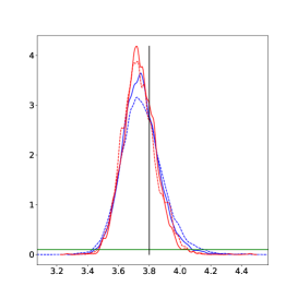
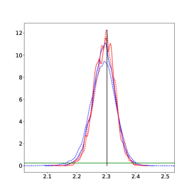
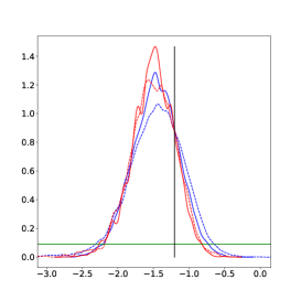
	True value	PMCMC	MCWM	DA-GP-MCMC	ADA-GP-MCMC
$\log r$	3.80	3.75 [3.53, 4.00]	3.75 [3.51, 4.05]	3.74 [3.54, 3.96]	3.73 [3.54, 3.97]
$\log\phi$	2.30	2.29 [2.21, 2.36]	2.29 [2.20, 2.37]	2.29 [2.23, 2.36]	2.29 [2.22, 2.36]
$\log\sigma$	-1.58	-1.47 [-2.13, -0.85]	-1.46 [-2.3, -0.75]	-1.5 [-2.12, -0.95]	-1.51 [-2.16, -0.92]

Table 2: Ricker model: Efficiency of PMCMC, MCWM, DA-GP-MCMC, and ADA-GP-MCMC. Timings for (A)DA-GP-MCMC do not include the training data collection and the fitting of the GP model.

	Seconds per 1000 iter.	Acceptance rate (%)	$\min$ ESS/sec	Skip DA run MH update (%)	Early- rejections (%)
PMCMC	20.26	40.21	2.53	NA	NA
MCWM	39.83	39.70	1.26	NA	NA
DA-GP-MCMC	10.32	7.66	1.99	14.75	81.05
ADA-GP-MCMC	9.46	7.89	1.75	15.02	80.49

Table 3: Ricker model: Estimated probabilities for the different cases and percentage of times the assumption for the different cases in the ADA-GP-MCMC algorithm holds.

	Case 1	Case 2	Case 3	Case 4
Est. probab. ($\hat{p}_{1}$,$\hat{p}_{2}$,$\hat{p}_{3}$,$\hat{p}_{4}$)	0.59	0.91	0.41	0.09
Perc. assum. holds (%)	73.51	88.24	39.80	21.21

Properties of the algorithms are presented in Table 2. Before discussing these results, we emphasize that the benefits of our accelerated procedure are to be considered when the case study has a likelihood that is computationally very challenging, and this is not the case for the present example, see instead Section 5.2. The ADA-GP-MCMC algorithm is the fastest algorithm, though only marginally faster than DA-GP-MCMC (4.2 times faster than MCWM and 1.09 times faster than DA-GP-MCMC), while MCWM is the slowest one. Not surprisingly, PMCMC is almost twice as fast as MCWM, and this is because PMCMC only requires one evaluation of the particle filter per iteration, while the MCWM requires two evaluations. The four algorithms are, however, essentially equally efficient, as from the $\min$ ESS/sec values.

The estimated probabilities $\hat{p}_{j}$ for the four different cases characterizing ADA-GP-MCMC (recall that $\hat{p}_{3}=1-\hat{p}_{1}$ and $\hat{p}_{4}=1-\hat{p}_{2}$), and the percentage for each case to hold, i.e. the probability that the selected case indeed is the correct one, are presented in Table 3. We notice that the probability for the different cases vary considerably, and also that the percentages that the assumption holds vary for the different cases. We also notice that the performance of the selection algorithm is much better for case 2 than for case 4: this is due to the unbalance of the two classes, meaning that in our training data case 2 occurs more frequently than case 4, and therefore it is more difficult to estimate the latter case accurately.

5.2 Double-well potential stochastic differential equation model for protein folding data

We now consider a computationally intensive case study concerning statistical inference for protein folding data. The challenges for this case study are: (a) the sample size is large, data being a long time-series (about $2.5\times 10^{4}$ observations), (b) the non-linear dynamics, and (c) the presence of local perturbations. “Protein folding” is the last and crucial step in the transformation of genetic information, encoded in DNA, into a functional protein molecule. Studying the time-dynamics of real protein folding dynamics results in a very high dimensional problem, which is difficult to analyze using exact Bayesian methodology. Therefore, for reasons of simplification and tractability, the dynamics of a protein are often modelled as diffusions along a single “reaction coordinate”, that is one-dimensional diffusion models are considered to model a projection of the actual dynamics in high-dimensional space (Best and Hummer, 2011).

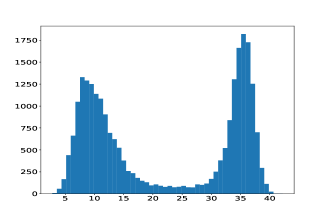
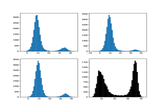
The (reaction coordinate) data is in Figure 2. We notice that data have a marginal bimodal structure, with irregular change-points where the mean of the data shifts, and a local noisy structure. A class of models shown to be suitable for statistical modeling of protein folding (at least when these data result into a low-dimensional projection of the original data) is given by stochastic differential equations (SDEs), see Forman and Sørensen (2014) and Picchini and Forman (2016). Monte Carlo inference methods are very computationally intensive for these models (in Picchini and Forman, 2016 data sub-sampling and special approximate Bayesian computation methods were used to accelerate the inference problem). We now introduce a novel double-well potential stochastic differential equation (DWP-SDE) model for protein folding data. This model is faster to simulate than the one proposed in Forman and Sørensen (2014) and Picchini and Forman (2016).

(a)

(b)

Figure 2: Data time course (left) and its marginal distribution (right).

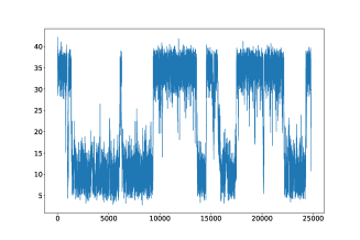
The DWP-SDE model is defined as

$$\begin{cases}z_{t}=x_{t}+y_{t},\\ dx_{t}=-\nabla V(x_{t})\,dt+\sigma\,dW^{x}_{t},\\ dy_{t}=-\kappa y_{t}\,dt+\sqrt{2\kappa\gamma^{2}}\,dW_{t}^{y}.\end{cases}$$ (9)

Here $\{z_{t}\}$ is the observable process, consisting in the sum of the solutions to the double-well potential SDE process $\{x_{t}\}$ and process $\{y_{t}\}$, the latter being unobservable and representing autocorrelated error. Here $\nabla V(\cdot)$ is the gradient of the double-well potential function $V(\cdot)$ with respect to $x_{t}$, further specified by six parameters introduced in (10). Finally $W_{t}^{X}$ and $W_{t}^{Y}$ are independent standard Wiener processes, that is their increments $dW_{t}^{X}$ and $dW_{t}^{Y}$ are independent, Gaussian distributed with zero mean and variance $dt$. We consider the following double-well potential function

$$V(x)=\frac{1}{2}\Big{\lvert}\frac{1}{2}\lvert x-c\rvert^{p_{1}}-d+gx\Big{\rvert}^{p_{2}}+\frac{1}{2}Ax^{2},$$ (10)

which is based on the potential described in equation 1 in Fang et al. (2017). The formulation in (10) is fairly general, in the sense that many different potentials can be specified by varying its parameters. The parameters in (10) have the following interpretation: $c$ specifies the location for the potential (i.e. where the potential is centered); $d$ determines the spread of the potential; $A$ is an asymmetry parameter; $g$ compresses the two modes of the long term (stationary) density of process $\{X_{t}\}$; parameters $p_{1}$ and $p_{2}$ control the shape of the two modes (if the parameters $p_{1}$ and $p_{2}$ are set to low values the long term probability distribution becomes more flat with less distinct modes); $\sigma$ governs the noise in the latent $\{X_{t}\}$ process. The error-model $Y_{t}$ is an Ornstein-Uhlenbeck process specified by two parameters: $\kappa$ is the autocorrelation level, and $\gamma$ is the noise intensity. In principle, inference should be conducted for $[\log\kappa,\log\gamma,\log A,\log c,\log d,\log g,\log p_{1},\log p_{2},\log\sigma]$. However, the model parameters $A$ and $g$ are “stiff”, i.e. small changes in their values result in considerable changes in the output, and are therefore hard to estimate. Estimating all the parameters of the DWP-SDE model is also a complex task since a larger data set seems needed to capture the stationary distribution of the data. We will therefore consider the easier task of estimating the parameters $\theta=[\log\kappa,\log\gamma,\log c,\log d,\log p_{1},\log p_{2},\log\sigma]$. The remaining parameters, $A$ and $g$, will be fixed to arbitrary values, as discussed later.

Simulating the $y_{t}$ process in (9) is easy since the transition density for the Ornstein-Uhlenbeck process process is known. We have that

$$y_{t+\Delta_{t}}|y_{t}=x\sim\mathcal{N}(xe^{-\kappa\Delta_{t}},\gamma^{2}(1-e^{-2\kappa\Delta_{t}})),$$

where $\Delta_{t}>0$. The transition density for the $x_{t}$ process is not analytically known, and we use the Euler-Maruyama scheme to propagate the $x_{t}$ process, that is we use

$$x_{t+\delta_{t}}|x_{t}=x\approx x-\nabla V(x)\delta_{t}+\sigma\epsilon_{t},$$

where $\epsilon_{t}\sim\mathcal{N}(0,\delta_{t}^{2})$, and $\delta_{t}>0$ is the stepsize for the Euler-Maruyama numerical integration scheme (typically $\delta_{t}\ll\Delta_{t}$).

Let us now consider the likelihood function for the $z_{t}$ process in (9), for a set of discrete observations $z=[z_{1},\ldots,z_{T}]$ that we assume observed at integer sampling times $t\in[1,2,...,T]$. Corresponding (unobservable) values for the $X_{t}$ process at the same sampling times are $[x_{1},\ldots,x_{T}]$. In addition, we denote with $x$ the set $x=[x_{0},x_{1},...,x_{T}]$, which includes an arbitrary value $x_{0}$ from which simulations of the latent system are started. The likelihood function can be written as

$$L(\theta) =p(z|\theta)=p(z_{1}|\theta)\prod_{t=2}^{T}p(z_{t}|z_{1},\ldots,z_{t-1},\theta),$$

$$=\int p(z_{1},\ldots,z_{T}|x_{0},\ldots x_{T},\theta)p(x_{0},\ldots,x_{T}|\theta)dx_{0}\cdots x_{T},$$

$$=\int p(z_{1},\ldots,z_{T}|x_{0},\ldots x_{T},\theta)p(x_{0})\prod_{t=1}^{T}p(x_{t}|x_{t-1},\theta)dx_{0}\cdots x_{T}.$$

The last product in the integrand is due to the Markov property of $X_{t}$. Also, we have introduced a density $p(x_{0})$, and if $x_{0}$ is deterministically fixed (as in our experiments) this density can be discarded. We cannot compute the likelihood function analytically (as the integral is typically intractable), but we can use sequential Monte Carlo (for example, the bootstrap filter in supplementary material) to compute an unbiased approximation $\hat{p}(z|\theta)$, which allows us to use PMCMC or MCWM for the inference. Furthermore, the $Z_{t}$ process is a transformation of the measurement noise that follows an Ornstein-Uhlenbeck process, and the density for $p(z_{1},\ldots,z_{T}|x_{0},\ldots x_{T},\theta)$ is known (Picchini and Forman, 2016). We have that

$$p(z_{1},\ldots,z_{T}|x_{0},\ldots x_{T},\theta)=\frac{1}{\gamma}\cdot\phi\Big{(}\frac{z_{1}-x_{1}}{\gamma}\Big{)}\cdot\prod_{t=2}^{T}\frac{1}{\gamma\sqrt{1-e^{-2\kappa\Delta_{t}}}}\cdot\phi\Big{(}\frac{z_{t}-x_{t}-e^{-\kappa\Delta_{t}}(z_{t-1}-x_{t-1})}{\gamma\sqrt{1-e^{-2\kappa\Delta_{t}}}}\Big{)},$$

where $\Delta_{t}=t_{i}-t_{i-1}$, and $\phi(\cdot)$ denotes the density function for the standard Gaussian distribution.

We now explain how an unbiased approximation to $p(z|\theta)$ is computed. To facilitate this explanation we introduce the following notation: let $x_{t-1}^{1:N}$ denote the set of $N$ particles we have at time $t-1$ before resampling is performed (see the bootstrap filter algorithm in the supplementary material). Let $\tilde{x}_{t-1}^{1:N}$ denote the resampled particles that are used to propagate the latent system forward to time $t$ (using Euler-Maruyama). We approximate $p(z|\theta)$ unbiasedly with $\hat{p}(z|\theta)$ as

$$\hat{p}(z|\theta)=\hat{p}(z_{1}|\theta)\prod_{t=2}^{T}\hat{p}(z_{t}|z_{1},\ldots,z_{t-1},\theta)=\hat{p}(z_{1}|\theta)\biggl{\{}\prod_{t=2}^{T}\frac{1}{N}\sum_{n=1}^{N}w_{t}^{n}\biggr{\}},$$

where the weights $w_{t}^{n}$ are

$$w_{t}^{n}=\frac{1}{\gamma\sqrt{1-e^{-2\kappa\Delta_{t}}}}\cdot\phi\Big{(}\frac{z_{t}-x_{t}^{n}-e^{-\kappa\Delta_{t}}(z_{t-1}-\tilde{x}^{n}_{t-1})}{\gamma\sqrt{1-e^{-2\kappa\Delta_{t}}}}\Big{)},\qquad t\geq 2$$

and

$$\hat{p}(z_{1}|\theta)=\frac{1}{N}\sum_{n=1}^{N}w_{1}^{n},\,\,\,\,\,\text{with}\,\,\,\,\,w_{1}^{n}=\frac{1}{\gamma}\cdot\phi\Big{(}\frac{z_{1}-\tilde{x}^{n}_{1}}{\gamma}\Big{)}.$$

5.2.1 Inference for protein folding data

We now consider the data in Figure 2. We fixed $A$ and $g$ to $A=-0.0025$ and $g=0$ as these parameters are difficult to identify, as already mentioned. Ideally, we should estimate $A$ and $g$, however, the data that we have access to seem to be not informative enough to infer all parameters simultaneously. We set Gaussian priors as follows (notice these are not really motivated by biophysical considerations, we just set priors to be weakly informative): $p(\log\kappa)\sim\mathcal{N}(-0.7,0.8^{2})$, $p(\log\gamma)\sim\mathcal{N}(-0.7,0.8^{2})$, $p(\log c)\sim\mathcal{N}(3.34,0.173^{2})$, $p(\log d)\sim\mathcal{N}(2.3,0.4^{2})$, $p(\log p_{1})\sim\mathcal{N}(0,0.5^{2})$, $p(\log p_{2})\sim\mathcal{N}(0,0.5^{2})$, and $p(\log\sigma)\sim\mathcal{N}(0.69,0.5^{2})$. The starting parameter values were set to $\exp(\theta_{0})=[0.5,2,20,15,1.5,1.5,2.5]$.

We use MCWM, DA-GP-MCMC, and ADA-GP-MCMC to estimate the unknown parameters. For each iteration of MCWM we compute 4 unbiased approximations of the likelihood function, one for each core of our computer, using $N=250$ particles for each of the 4 likelihoods. Taking the sample average of these likelihoods produces another unbiased estimate of the likelihood, but with a smaller variance than the individual ones (this is obviously true and also studied in detail in Drovandi, 2014). However, given the length of the time-series, the obtained approximated likelihood is still fairly variable, and should we use PMCMC this would produce sticky chains. Therefore MCWM comes to our help for this example, as “refreshing” the denominator of the acceptance ratio helps escaping from sticky points, occurring when the likelihood approximation is overestimated.

We used the following settings with MCWM: 20,000 iterations in total and a burnin of 10,000 iterations. The proposal distribution used the generalized AM algorithm, set to target an acceptance rate of 15%. The training part for DA-GP-MCMC and ADA-GP-MCMC was the output of an MCWM algorithm with the settings specified above. We fit a GP model to the output from the first 5,000 iterations of MCWM obtained after burnin. In a similar manner as for the Ricker model the two transition kernels $g$ and $\tilde{g}$ were based on the covariance matrices returned by the final iteration of the MCWM algorithm. A decision tree model, similar to the one used for the Ricker model, was used for the selection problem. Then we ran DA-GP-MCMC and ADA-GP-MCMC for 10,000 iterations, using $\beta_{MH}=0.15$. Same as with the Ricker model, a MCWM-style updating scheme was used in the second stage of both DA and ADA algorithms.

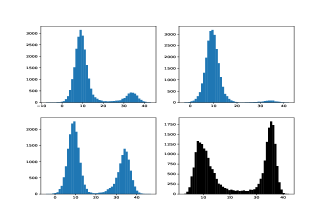
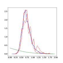
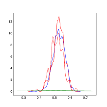
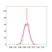
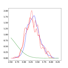
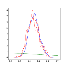
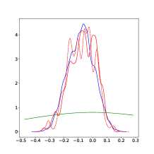
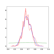
Marginal posteriors are in Figure 4, and inference results are in Table 4 and, same as for the Ricker model, we conclude that all three algorithms generate similar posterior inference. Algorithmic properties are in Table 5, and we conclude that in this case we obtain a higher speed-up compared to the Ricker model. Results are commented in detail in section 5.3. The estimated probabilities for the selection of the four different cases are in Table 6, and we observe that case 4 is the least likely case. Similarly as for the Ricker model, and due to the same reasons, the performance of the selection algorithm is much better for case 2 than for case 4.

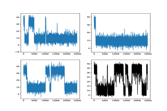
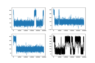
To further illustrate inference results, we randomly pick posterior draws from the high-density region of the posterior distribution, and conditionally to these we run forward simulations using the model in (9). In Figure 3 we show three such forward simulations obtained from parameters sampled via MCMW and ADA-GP-MCMC. These look similar, which is not surprising since the posterior distribution that we obtain for the two methods also are similar. The number of regime switches appears underestimated compared to data. The forward simulations also show that we over-estimate the probability mass in the folded regime. This is likely due to not having estimated $A$ and $g$ from data. The values set for these two parameters are likely suboptimal, and (conditionally to those) the resulting inference for the remaining parameters is probably biased. We believe we require a longer dataset to be able to fit correctly all parameters, including $A$ and $g$.

Table 4: DWP-SDE model: Posterior means (2.5th and 97.5th quantiles) for MCWM, DA-GP-MCMC, and ADA-GP-MCMC.

	MCWM	DA-GP-MCMC	ADA-GP-MCMC
$\log\kappa$	0.73 [0.42,1.19]	0.74 [0.45,1.12]	0.76 [0.42,1.29]
$\log\gamma$	0.53 [0.45,0.59]	0.52 [0.44,0.6]	0.52 [0.44,0.59]
$\log c$	3.09 [3.08,3.11]	3.1 [3.08,3.1]	3.1 [3.08,3.11]
$\log d$	3.36 [2.94,3.84]	3.32 [2.89,3.89]	3.32 [2.91,3.81]
$\log p_{1}$	0.46 [0.35,0.57]	0.45 [0.34,0.58]	0.45 [0.34,0.56]
$\log p_{2}$	-0.08 [-0.26, 0.09]	-0.07 [-0.26,0.08]	-0.08 [-0.25,0.07]
$\log\sigma$	0.68 [0.56,0.8]	0.68 [0.57,0.78]	0.69 [0.57,0.82]

Table 5: DWP-SDE model: Efficiency of MCWM, DA-GP-MCMC, and ADA-GP-MCMC. Timings for (A)DA-GP-MCMC do not include the training data collection and the fitting of the GP model.

	Minutes per 1000 iter.	Acceptance rate (%)	$\min$ ESS/min	Second stage direct (%)	Early- rejections (%)
MCWM	75.88	18.5	0.39	NA	NA
DA-GP-MCMC	24.81	3.96	0.69	15.27	68.95
ADA-GP-MCMC	15.37	3.34	0.94	14.52	69.21

Table 6: DWP-SDE model: Estimated probabilities for the different cases and percentage of times the assumption for the different cases in the ADA-GP-MCMC algorithm holds.

	Case 1	Case 2	Case 3	Case 4
Est. prob.	0.22	0.91	0.78	0.09
Perc. assum. holds (%)	43.14	87.67	65.92	25.38

(a)

(b)

(c)

(d)

Figure 3: Trajectories in blue are forward simulated from the DWP-SDE using draws from MCWM (a) and ADA-GP-MCMC (c). Black trajectories are data. Corresponding marginal distributions from MCWM (b) and ADA-GP-MCMC (d).

(a) $\log\kappa$.

(b) $\log\gamma$.

(c) $\log c$.

(d) $\log d$.

(e) $\log p_{1}$.

(f) $\log p_{2}$.

(g) $\log\sigma$.

Figure 4: Marginal posteriors for the DWP-SDE model: MCWM (blue solid line), DA-GP-MCMC (red solid line), and ADA-GP-MCMC (red dashed line). Priors are denoted with green lines (these look “cut” as we zoom on the bulk of the posterior).

5.3 Analysis of ADA-GP-MCMC

In the following we simplify the notation and refer to ADA-GP-MCMC and DA-GP-MCMC as ADA and DA. To analyze the runtime speed-up produced by ADA we execute multiple runs of both DA and ADA. We focus on four metrics measured over 1,000 MCMC iterations: runtimes for DA and ADA; the speed-up attained by ADA, expressed as how much faster ADA is in comparison with DA; the number of particle filter evaluations in the second stage for DA and ADA (notice, in the DA case this corresponds exactly to the number of times the second stage is reached); the reduction in the number of particle filter evaluations for ADA compared to DA. Since we are interested in analyzing the speed-up potential of ADA and not necessarily the inference results we set $\beta_{MH}=0$, hence, we never skip the ADA/DA part of the algorithms.

Furthermore, we run our analyses independently on 100 simulated datasets (see the supplementary material) using 1200 particles equally distributed across 4 cores. Results are in Figure 5. We conclude that ADA is about 2 to 4 times as fast as DA. The number of particle filter evaluations for ADA is reduced by a factor of about 3.

(a)

(b)

(c)

(d)

Figure 5: Speed-up analysis for the DWP model across 100 independent simulations, each for 1000 iterations, using the simulated data set. Subfigures: a) Run-times (sec) for DA (left boxplot) and ADA (right boxplot); b) Speed-up of ADA relative to DA; c) Number of particle filter evaluations in the second stage of DA (left) and ADA (right); d) Reduction in number of particle filter evaluations in the second stage for ADA compared to DA.

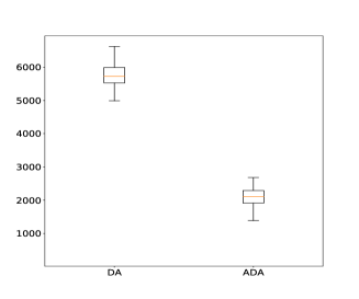
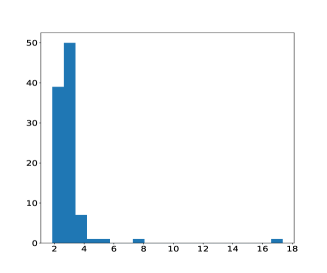
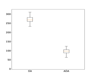
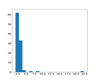
Regarding ADA, it is interesting to study how often each of the four possible cases illustrated in Section 2.1 are selected, and how likely it is that we run a particle filter conditionally on the selected case. Table 7 reports our findings for the Ricker model and DWP-SDE. We notice that proposals are not equally likely to be sent to each of the four cases, and that case 4 is the least likely case for a proposal to be sent to. It is perhaps surprising to observe the marked difference in the percentages of proposals sent to case 3 and case 4, as both cases correspond to likelihood ratios (ratio of GP likelihoods and ratio of particle filter likelihoods) that disagree in sign at the evaluated proposal. Furthermore, we can also conclude that the probability of running the particle filter varies for the different cases. Not surprisingly, given how the cases are defined, the probability for case 2 is 1 and is 0 for case 4. We also note that the probability of running the particle filter in case 3 is much lower compared to case 1: this means that whenever case 1 is selected for proposal $\theta^{\star}$ it turns that the event $u<\tilde{L}(\theta^{r-1})/\tilde{L}(\theta^{\star})$ is less likely than the event having the opposite inequality. If instead case 3 is selected, event $u>\frac{\tilde{L}(\theta^{r-1})}{\tilde{L}(\theta^{\star})}$ is less likely than the event having the opposite inequality.

Table 7: Percentage of proposals sent to the different cases (mean over 100 iterations of the ADA-MCMC algorithm), and probability of running the particle filter given the specific selected case (mean over 100 iterations of the ADA-MCMC algorithm).

	Percentage of proposals in each case (%)					Prob. of running particle filter in each case
	Case 1	Case 2	Case 3	Case 4		Case 1	Case 2	Case 3	Case 4
Ricker model	62.59	12.61	21.31	3.59		0.82	1	0.40	0
DWP-SDE protein folding data.	18.80	6.82	73.28	1.09		0.98	1	0.024	0

6 Summary

We have provided ways to speed up MCMC sampling by introducing a novel, approximate version of the so-called “delayed-acceptance” MCMC introduced in Christen and Fox (2005). More specifically, our ADA-MCMC algorithm can be used to accelerate MCMC sampling for Bayesian inference by exploiting possibilities to avoid the evaluation of a computationally expensive likelihood function. While the standard DA-MCMC only accepts proposals by evaluating the likelihood function associated to the exact posterior, instead ADA-MCMC in some specific cases can accept proposals even without the evaluation of the likelihood. Clearly, this is particularly relevant in statistical experiments where the likelihood function is not analytically available and is expensive to approximate. This is typical when unbiased approximations of the likelihood are used in pseudo-marginal algorithms for exact Bayesian inference (Andrieu and Roberts, 2009). Another situation where ADA-MCMC comes useful is when the likelihood function turns expensive due to the size of the data.

Both DA-MCMC and ADA-MCMC depend on the construction of surrogates of the likelihood function. Unfortunately, producing a useful (i.e. informative) surrogate of the likelihood has its own cost. In fact, the construction of the surrogate model is typically the result of a “learning” procedure, where the output of a preliminary MCMC run (obtained using the expensive likelihood) is used to understand the relationship between simulated parameters and simulated data (e.g. using neuronal-networks as in Papamakarios et al., 2018), or between simulated log-likelihoods and parameter proposals (as in Drovandi et al., 2018).

ADA-MCMC samples from an approximate posterior distribution, while the original DA-MCMC algorithm is an exact algorithm. However, our case studies suggest that the approximative posterior inference returned by ADA-MCMC is close to the one obtained with DA-MCMC and Markov-chain-within-Metropolis (MCWM). This result is possibly connected with the quality of the surrogate model. If a poor surrogate model was used, the inference obtained using ADA-MCMC could be biased compared to DA-MCMC. The reason for this is that, in some cases, ADA-MCMC allows us to accept a proposal merely based on the surrogate model.

ADA-MCMC only generates an acceleration in the computations if the evaluation of the likelihood is time-consuming. If this evaluation is relatively fast, ADA-MCMC does not bring any significant gain compared to DA-MCMC (and in this case, any delayed-acceptance procedure should not be considered in the first place). An example of the latter case is shown with the Ricker model case study. However, for the DWP-SDE model, each likelihood evaluation using a particle filter requires about 2-10 seconds, depending on how many particles we use, and the benefits of using our novel approach are clear. Also, for this specific application, the expensive particle filter is invoked 2 to 5 times less often for ADA-MCMC than for DA-MCMC.

ADA-MCMC is not limited to the Bayesian setting and can be used to sample from a generic distribution, as mentioned in Section 2.1. Furthermore, when considering the inference problem in a Bayesian setting, ADA-MCMC can straightforwardly be paired with some other surrogate model than the Gaussian process regression model we employ. Hence, ADA-MCMC is a general algorithm for Monte Carlo sampling that can be exploited in multiple ways, other than the ones we have illustrated.

SUPPLEMENTARY MATERIAL

Further methodological tools:

Details on PMCMC, MCWM, the bootstrap filter, GP regression, diagnostics, further simulation studies and setup for the implementations. (PDF file).

Julia code:

the Julia code used to run the experiments is available at:
https://github.com/SamuelWiqvist/adamcmcpaper.

See pages - of sup_mat.pdf

References

- Andrieu and Roberts [2009] C. Andrieu and G. O. Roberts. The pseudo-marginal approach for efficient Monte Carlo computations. The Annals of Statistics, 37:697–725, 2009.
- Andrieu and Thoms [2008] C. Andrieu and J. Thoms. A tutorial on adaptive MCMC. Statistics and Computing, 18(4):343–373, 2008.
- Angelino et al. [2016] E. Angelino, M. J. Johnson, R. P. Adams, et al. Patterns of scalable Bayesian inference. Foundations and Trends® in Machine Learning, 9(2-3):119–247, 2016.
- Banterle et al. [2015] M. Banterle, C. Grazian, A. Lee, and C. P. Robert. Accelerating metropolis-hastings algorithms by delayed acceptance. arXiv preprint arXiv:1503.00996, 2015.
- Best and Hummer [2011] R. B. Best and G. Hummer. Diffusion models of protein folding. Physical Chemistry Chemical Physics, 13(38):16902–16911, 2011.
- Christen and Fox [2005] J. A. Christen and C. Fox. Markov chain Monte Carlo using an approximation. Journal of Computational and Graphical statistics, 14(4):795–810, 2005.
- Drovandi [2014] C. C. Drovandi. Pseudo-marginal algorithms with multiple CPUs. https://eprints.qut.edu.au/61505/, 2014.
- Drovandi et al. [2018] C. C. Drovandi, M. T. Moores, and R. J. Boys. Accelerating pseudo-marginal MCMC using Gaussian processes. Computational Statistics & Data Analysis, 118:1–17, 2018.
- Everitt and Rowińska [2017] R. G. Everitt and P. A. Rowińska. Delayed acceptance ABC-SMC. arXiv:1708.02230, 2017.
- Fang et al. [2017] S.-C. Fang, D. Y. Gao, G.-X. Lin, R.-L. Sheu, and W.-X. Xing. Double well potential function and its optimization in the -dimensional real space: part i. Journal of Industrial and Management Optimization, 13(3):1291–1305, 2017.
- Fasiolo et al. [2016] M. Fasiolo, N. Pya, and S. Wood. A comparison of inferential methods for highly nonlinear state space models in ecology and epidemiology. Statistical Science, 31(1):96–118, 2016.
- Fearnhead and Prangle [2012] P. Fearnhead and D. Prangle. Constructing summary statistics for approximate Bayesian computation: semi-automatic approximate Bayesian computation. Journal of the Royal Statistical Society: Series B, 74(3):419–474, 2012.
- Forman and Sørensen [2014] J. L. Forman and M. Sørensen. A transformation approach to modelling multi-modal diffusions. Journal of Statistical Planning and Inference, 146:56–69, 2014.
- Franks and Vihola [2017] J. Franks and M. Vihola. Importance sampling and delayed acceptance via a Peskun type ordering. arXiv:1706.09873, 2017.
- Golightly et al. [2015] A. Golightly, D. A. Henderson, and C. Sherlock. Delayed acceptance particle MCMC for exact inference in stochastic kinetic models. Statistics and Computing, 25(5):1039–1055, 2015.
- Hastings [1970] W. K. Hastings. Monte Carlo sampling methods using Markov chains and their applications. Biometrika, 57(1):97–109, 1970.
- Kantas et al. [2015] N. Kantas, A. Doucet, S. S. Singh, J. Maciejowski, and N. Chopin. On particle methods for parameter estimation in state-space models. Statistical Science, 30(3):328–351, 2015.
- Marin et al. [2012] J. Marin, P. Pudlo, C. Robert, and R. Ryder. Approximate Bayesian computational methods. Statistics and Computing, pages 1–14, 2012.
- Meeds and Welling [2014] E. Meeds and M. Welling. GPS-ABC: Gaussian process surrogate approximate Bayesian computation. In Proceeding of the 30th conference on Uncertainty in Artificial Intelligence (UAI), 2014.
- Mueller [2010] C. L. Mueller. Exploring the common concepts of adaptive MCMC and covariance matrix adaptation schemes. In A. Auger, J. L. Shapiro, L. D. Whitley, and C. Witt, editors, Theory of Evolutionary Algorithms. Schloss Dagstuhl - Leibniz-Zentrum für Informatik, Germany, 2010.
- Papamakarios et al. [2018] G. Papamakarios, D. C. Sterratt, and I. Murray. Sequential neural likelihood: Fast likelihood-free inference with autoregressive flows. arXiv preprint arXiv:1805.07226, 2018.
- Picchini [2014] U. Picchini. Inference for SDE models via approximate Bayesian computation. Journal of Computational and Graphical Statistics, 23(4):1080–1100, 2014.
- Picchini and Forman [2016] U. Picchini and J. L. Forman. Accelerating inference for diffusions observed with measurement error and large sample sizes using approximate Bayesian computation. Journal of Statistical Computation and Simulation, 86(1):195–213, 2016.
- Quiroz et al. [2017] M. Quiroz, M.-N. Tran, M. Villani, and R. Kohn. Speeding up MCMC by delayed acceptance and data subsampling. Journal of Computational and Graphical Statistics, 2017. doi: 10.1080/10618600.2017.1307117.
- Rasmussen and Williams [2006] C. E. Rasmussen and C. K. I. Williams. Gaussian processes for machine learning. MIT press, 2006.
- Rosenthal and Roberts [2007] J. Rosenthal and G. Roberts. Coupling and ergodicity of adaptive MCMC. Journal of Applied Probablity, 44:458–475, 2007.
- Schön et al. [2018] T. B. Schön, A. Svensson, L. Murray, and F. Lindsten. Probabilistic learning of nonlinear dynamical systems using sequential Monte Carlo. Mechanical Systems and Signal Processing, 104:866–883, 2018.
- Sherlock et al. [2017] C. Sherlock, A. Golightly, and D. A. Henderson. Adaptive, delayed-acceptance MCMC for targets with expensive likelihoods. Journal of Computational and Graphical Statistics, 26(2):434–444, 2017.
- Solonen et al. [2012] A. Solonen, P. Ollinaho, M. Laine, H. Haario, J. Tamminen, and H. Järvinen. Efficient MCMC for climate model parameter estimation: parallel adaptive chains and early rejection. Bayesian Analysis, 7(3):715–736, 2012.
- Wood [2010] S. N. Wood. Statistical inference for noisy nonlinear ecological dynamic systems. Nature, 466(7310):1102–1104, 2010.