Uncertainty Estimations by Softplus normalization in Bayesian Convolutional Neural Networks with Variational Inference
Abstract
We introduce a novel uncertainty estimation for classification tasks for Bayesian convolutional neural networks with variational inference. By normalizing the output of a Softplus function in the final layer, we estimate aleatoric and epistemic uncertainty in a coherent manner. The intractable posterior probability distributions over weights are inferred by Bayes by Backprop. Firstly, we demonstrate how this reliable variational inference method can serve as a fundamental construct for various network architectures. On multiple datasets in supervised learning settings (MNIST, CIFAR-10, CIFAR-100), this variational inference method achieves performances equivalent to frequentist inference in identical architectures, while the two desiderata, a measure for uncertainty and regularization are incorporated naturally. Secondly, we examine how our proposed measure for aleatoric and epistemic uncertainties is derived and validate it on the aforementioned datasets.
1 Introduction
Convolutional neural networks excel at tasks in the realm of image classification (e.g. [1, 2, 3]). However, from a probability theory perspective, it is unjustifiable to use single point-estimates as weights to base any classification on. Cnns with frequentist inference require substantial amounts of data examples to train on and are prone to overfitting on datasets with few examples per class.
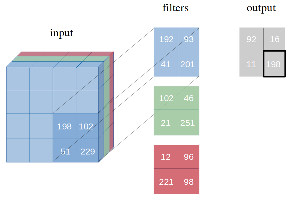
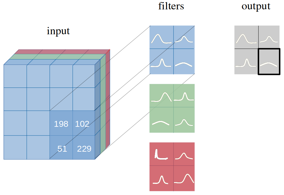
In this work, we apply Bayesian methods to Cnns in order to add a measure for uncertainty and regularization in their predictions, respectively their training. This approach allows the network to express uncertainty via its parameters in form of probability distributions (see Figure 1). At the same time, by using a prior probability distribution to integrate out the parameters, we compute the average across many models during training, which gives a regularization effect to the network, thus preventing overfitting.
We build our Bayesian Cnn upon Bayes by Backprop [4, 5], and approximate the intractable true posterior probability distributions with variational probability distributions , which comprise the properties of Gaussian distributions and , denoted , where is the total number of parameters defining a probability distribution. The shape of these Gaussian variational posterior probability distributions, determined by their variance , expresses an uncertainty estimation of every model parameter. The main contributions of our work are as follows:
-
1.
We present how Bayes by Backprop can be efficiently applied to Cnns. We therefore introduce the idea of applying two convolutional operations, one for the mean and one for the variance.
-
2.
We empirically show how this generic and reliable variational inference method for Bayesian Cnns can be applied to various Cnn architectures without any limitations on their performances, but with intrinsic regularization effects. We compare the performances of these Bayesian Cnns to Cnns which use single point-estimates as weights, i.e. which are trained by frequentist inference.
-
3.
We explain and implement Softplus normalization by means of examining how to estimate aleatoric and epistemic uncertainties without employing an additional Softmax function in the output layer [6] which brings an inconsistency of activation functions into the model.
This paper is structured as subsequently outlined: after we have introduced our work here, we secondly review Bayesian neural networks with variational inference, including previous works, an explanation of Bayes by Backprop and its implementation in Cnn. Thirdly, we examine aleatoric and epistemic uncertainty estimations with an outline of previous works and how our proposed method directly connects to those. Fourthly, we present our results and findings through experimental evaluation of the proposed method on various architectures and datasets before we finally conclude our work.
2 Bayesian convolutional neural networks with variational inference
Recently, the uncertainty afforded by Bayes by Backprop trained neural networks has been used successfully to train feedforward neural networks in both supervised and reinforcement learning environments [5, 7, 8], for training recurrent neural networks [9], and for Cnns [10, 11]. Here, we review this method for Cnns to construct a common foundation on which be build on in section 3.
2.1 Related work
Applying Bayesian methods to neural networks has been studied in the past with various approximation methods for the intractable true posterior probability distribution . [12] started to propose various maximum-a-posteriori (MAP) schemes for neural networks. They were also the first who suggested second order derivatives in the prior probability distribution to encourage smoothness of the resulting approximate posterior probability distribution. In subsequent work by [13], the first variational methods were proposed which naturally served as a regularizer in neural networks. [14] suggest taking an information theory perspective into account and utilizing a minimum description length (MDL) loss. This penalises non-robust weights by means of an approximate penalty based upon perturbations of the weights on the outputs. [15] and [16] investigated the posterior probability distributions of neural networks by using Laplace approximations. As a response to the limitations of Laplace approximations, [17] investigated the use of hybrid Monte Carlo for training neural networks, although it has so far been difficult to apply these to the large sizes of neural networks built in modern applications. More recently, [4] derived a variational inference scheme for neural networks and [5] extended this with an update for the variance that is unbiased and simpler to compute. [18] derives a similar algorithm in the case of a mixture posterior probability distribution.
Several authors have derived how Dropout [19] and Gaussian Dropout [20] can be viewed as approximate variational inference schemes [21, 22]. We compare our results to [21]. Furthermore, structured variational approximations [23], auxiliary variables [24], and Stochastic Gradient MCMC [25] have been proposed to approximate the intractable posterior probability distribution. Recently, the uncertainty afforded by Bayes by Backprop trained neural networks has been used successfully to train feedforward neural networks in both supervised and reinforcement learning environments [5, 7, 8], for training recurrent neural networks [9], and convolutional neural networks [10, 11].
2.2 Bayes by Backprop
Bayes by Backprop [4, 5] is a variational inference method to learn the posterior distribution on the weights of a neural network from which weights can be sampled in backpropagation. Since the true posterior is typically intractable, an approximate distribution is defined that is aimed to be as similar as possible to the true posterior , measured by the Kullback-Leibler (KL) divergence [26]. Hence, we define the optimal parameters as
| (1) | ||||
where
| (2) |
This derivation forms an optimization problem with a resulting cost function widely known as variational free energy [27, 28, 29] which is built upon two terms: the former, , is dependent on the definition of the prior , thus called complexity cost, whereas the latter, , is dependent on the data , thus called likelihood cost.
The term can be omitted in the optimization because it is constant.
Since the KL-divergence is also intractable to compute exactly, we follow a stochastic variational method [4, 5].
We sample the weights from the variational distribution since it is much more probable to draw samples which are appropriate for numerical methods from the variational posterior than from the true posterior . Consequently, we arrive at the tractable cost function (3) which is aimed to be optimized, i.e. minimised with respect to , during training:
| (3) |
where is the number of draws. We sample from .
2.3 Bayes by Backprop for convolutional neural networks
In this section, we explain our algorithm of building Cnns with probability distributions over weights in each filter, as seen in Figure 1, and apply Bayes by Backprop to compute the intractable posterior probability distributions , as described in the previous section 2.2. Notably, a fully Bayesian perspective on a Cnn is for most Cnn architectures not accomplished by merely placing probability distributions over weights in convolutional layers; it also requires probability distributions over weights in fully-connected layers.
2.3.1 Local reparameterization trick for convolutional layers
We utilize the local reparameterization trick [22] and apply it to Cnns. Following [22, 11], we do not sample the weights , but we sample layer activations instead due to its consequent computational acceleration. The variational posterior probability distribution (where and are the input, respectively output layers, and the height, respectively width of any given filter) allows to implement the local reparamerization trick in convolutional layers. This results in the subsequent equation for convolutional layer activations :
| (4) |
where , is the receptive field, signalises the convolutional operation, and the component-wise multiplication.
2.3.2 Applying two sequential convolutional operations (mean and variance)
The crux of equipping a Cnn with probability distributions over weights instead of single point-estimates and being able to update the variational posterior probability distribution by backpropagation lies in applying two convolutional operations whereas filters with single point-estimates apply one. As explained in the previous section 2.3.1, we deploy the local reparametrization trick and sample from the activations . Since activations are functions of mean and variance among others, we are able to compute the two variables determining a Gaussian probability distribution, mean and variance , separately.
We pursue this in two convolutional operations: in the first, we treat the output as an output of a Cnn updated by frequentist inference. We optimize with Adam [30] towards a single point-estimate which makes the accuracy of classifications in the validation dataset increasing. We interpret this single point-estimate as the mean of the variational posterior probability distributions . In the second convolutional operation, we learn the variance . As this formulation of the variance includes the mean , only needs to be learned in the second convolutional operation [31]. In this way, we ensure that only one parameter is updated per convolutional operation, exactly how it would have been with a Cnn updated by frequentist inference.
In other words, while we learn in the first convolutional operation the MAP of the variational posterior probability distribution , we observe in the second convolutional operation how much values for weights deviate from this MAP. This procedure is repeated in the fully-connected layers. In addition, to accelerate computation, to ensure a positive non-zero variance , and to enhance accuracy, we learn and use the Softplus activation function as further described in the Experiments section 4.
3 Uncertainty estimation in Bayesian Cnns
In classification tasks, we are interested in the predictive distribution , where is an unseen data example and its predicted class. For a Bayesian neural network, this quantity is given by:
| (5) |
In Bayes by Backprop, Gaussian distributions , where are learned with some dataset as we explained previously in 2.2. Due to the discrete and finite nature of most classification tasks, the predictive distribution is commonly assumed to be a categorical. Incorporating this aspect into the predictive distribution gives us
| (6) | ||||
where is the total number of classes and .
As there is no closed-form solution due to the lack of conjugacy between categorical and Gaussian distributions, we cannot recover this distribution. However, we can construct an unbiased estimator of the expectation by sampling from :
| (7) |
where is the predefined number of samples. This estimator allows us to evaluate the uncertainty of our predictions by the definition of variance, hence called predictive variance and denoted as :
| (8) | ||||
where and .
It is important to split the uncertainty in form of the predictive variance into aleatoric and epistemic quantities since it allows the modeler to evaluate the room for improvements: while aleatoric uncertainty (also known as statistical uncertainty) is merely a measure for the variation of ("noisy") data, epistemic uncertainty is caused by the model. Hence, a modeler can see whether the quality of the data is low (i.e. high aleatoric uncertainty), or the model itself is the cause for poor performances (i.e. high epistemic uncertainty). The former can be improved by gathering more data, whereas the latter requests to refine the model [32].
3.1 Related work
As shown in (8), the predictive variance can be decomposed into the aleatoric and epistemic uncertainty. [33] and [6] have proposed disparate methods to do so. In this paragraph, we first review these two methods before we explain our own method and how it overcomes deficiencies of the two aforementioned ones, especially the usage of Softmax in the output layer by [6].
[33] derived a method how aleatoric and epistemic uncertainties can directly be estimated by constructing a Bayesian neural network with the last layer before activation consisting of mean and variance of logits, denoted and . In other words, the pre-activated linear output of the neural network has dimensions with being the number of output units, i.e. potential classes. They propose an estimator as
| (9) |
where . [6] mention the deficiencies of this approach: first, it models the variability of the linear predictors and and not the predictive probabilities; second, it ignores the fact that the covariance matrix of a multinomial random variable is a function of the mean vector; and third, the aleatoric uncertainty does not reflect correlations because of the diagonal matrix.
To overcome these deficiencies, [6] propose
| (10) |
where and . By doing so, they do not need the pre-activated linear outputs and . Consequently, they can directly compute the variability of the predictive probability and do not require additional sampling steps. With increasing , (10) converges in probability to (8).
3.2 Softplus normalization
Deploying the Softmax function assumes we classify according to the logistic sigmoid function:
| (11) | ||||
| (12) |
where the label is assigned to the input if . Assume we have classes, this logistic sigmoid function can be generalized to the Softmax function:
| (13) |
Here, we propose a novel method how aleatoric and epistemic uncertainty estimations can be computed without having an additional non-linear transformation by the generalized logistic sigmoid function in the output layer.
The predictive variance remains in the form as stated in (10), except the subsequent two amendments compared to [6]: we circumvent the exponential term in the Softmax function, hence generate consistency of activation functions in the entire Cnn. Despite not punishing wrong predictions particularly with the exponential term, we also resolve concerns about robustness by employing not more than one type of non-linear transformations within the same neural network while we preserve the desideratum of having probabilities as outputs. We implement this in two subsequent computations: first, we employ the same activation function in the output layer as we employ in any other hidden layer, namely the Softplus function, see (16); second, these outputs are normalized by dividing the output of each class by the sum of all outputs:
| (14) |
This procedure can be summarized as a replacement of with where is the aforementioned normalization of the Softplus output. We call this computation Softplus normalization. Our intuition for this is as follows: we classify according to a categorical distribution as we outlined previously in section 3. This can be seen as an approximation of the outputs with one-hot vectors. If those vectors already contain a lot of zeros, the approximation is going to be more accurate. For a Softmax, predicting zeros requires a logit of which is hard to achieve in practice. For the Softplus normalization, we just need a negative value roughly smaller than to get nearly a zero in the output. Consequently, Softplus normalization can easily produce vectors that are in practice zero, whereas Softmax cannot. In sum, our proposed method is as follows:
| (15) |
where and .
4 Experiments
For all conducted experiments, we implement the foregoing description of Bayesian Cnns with variational inference in LeNet-5 [34], AlexNet [3], and VGG [2]. The exact architecture specifications can be found in the Appendix 6 and in our GitHub repository111https://github.com/kumar-shridhar/PyTorch-Softplus-Normalization-Uncertainty-Estimation-Bayesian-CNN. We train the networks with the MNIST dataset of handwritten digits [34], and with the CIFAR-10 and CIFAR-100 datasets [35] since these datasets serve widely as benchmarks for Cnns’ performances. The originally chosen activation functions in all architectures are ReLU, but we must introduce another, called Softplus, see (16), because of our method to apply two convolutional or fully-connected operations. As aforementioned, one of these is determining the mean , and the other the variance . Specifically, we apply the Softplus function because we want to ensure that the variance never becomes zero. This would be equivalent to merely calculating the MAP, which can be interpreted as equivalent to a maximum likelihood estimation (MLE), which is further equivalent to utilising single point-estimates, hence frequentist inference. The Softplus activation function is a smooth approximation of ReLU. Although it is practically not influential, it has the subtle and analytically important advantage that it never becomes zero for , whereas ReLU becomes zero for .
| (16) |
where is by default set to .
All experiments are performed with the same hyper-parameters settings as stated in the Appendix 6.
4.1 Results of Bayesian CNNs with variational inference
| MNIST | CIFAR-10 | CIFAR-100 | |
|---|---|---|---|
| Bayesian VGG (with VI) | 99 | 86 | 45 |
| Frequentist VGG | 99 | 85 | 48 |
| \hdashlineBayesian AlexNet (with VI) | 99 | 73 | 36 |
| Frequentist AlexNet | 99 | 73 | 38 |
| \hdashlineBayesian LeNet-5 (with VI) | 98 | 69 | 31 |
| Frequentist LeNet-5 | 98 | 68 | 33 |
| \hdashlineBayesian LeNet-5 (with Dropout) | 99 | 83 |
We evaluate the performance of our Bayesian Cnns with variational inference. Table 1 shows a comparison of validation accuracies (in percentage) for architectures trained by two disparate Bayesian approaches, namely variational inference, i.e. Bayes by Backprop and Dropout as proposed by Gal and Ghahramani [21], plus frequentist inference for all three datasets. Bayesian Cnns trained by variational inference achieve validation accuracies comparable to their counter-architectures trained by frequentist inference. On MNIST, validation accuracies of the two disparate Bayesian approaches are comparable, but a Bayesian LeNet-5 with Dropout achieves a considerable higher validation accuracy on CIFAR-10, although we were not able to reproduce these reported results.
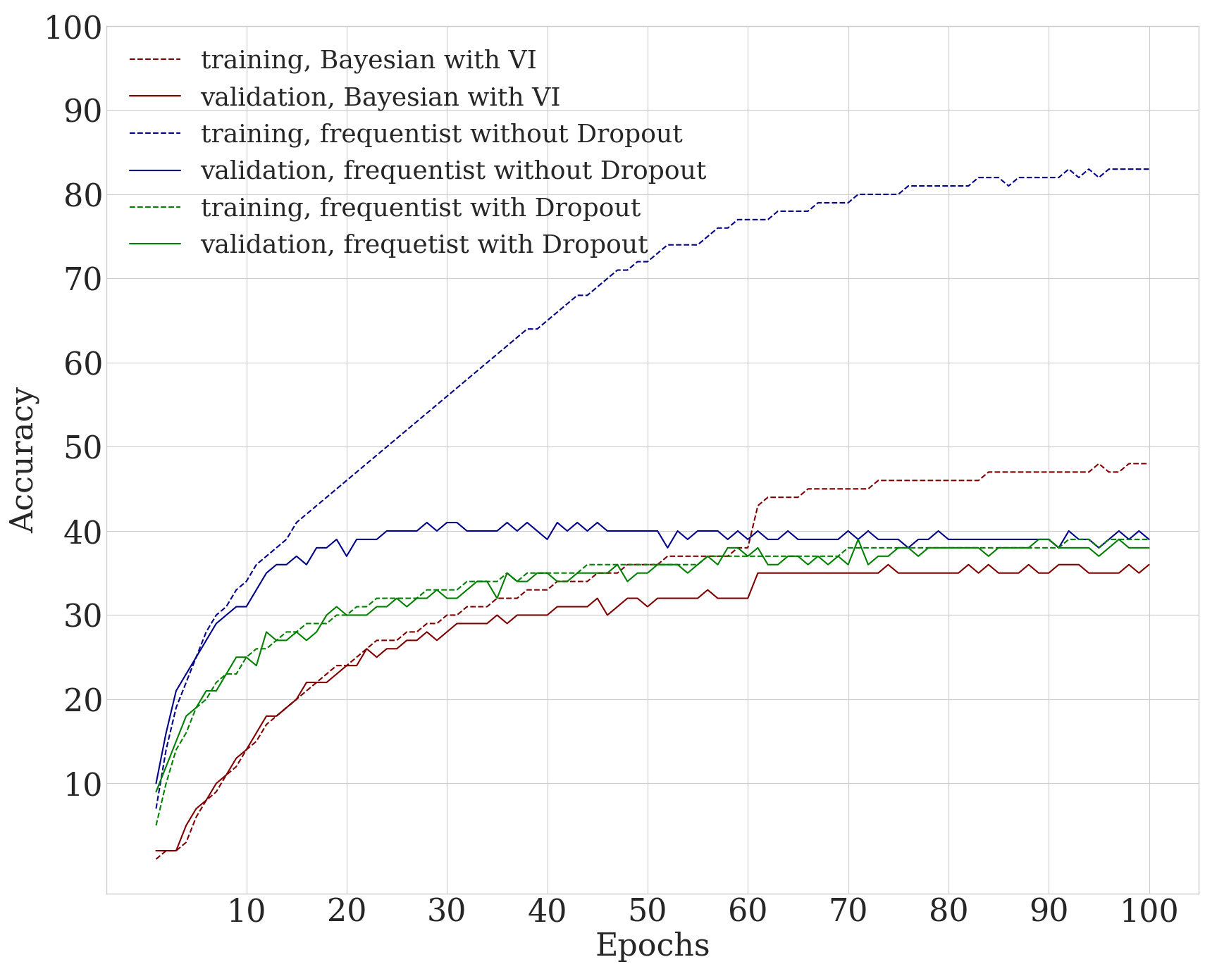
In Figure 2, we show how Bayesian networks incorporate naturally effects of regularization, exemplified on AlexNet. While an AlexNet trained by frequentist inference without any regularization overfits greatly on CIFAR-100, an AlexNet trained by Bayesian inference on CIFAR-100 does not. It performs equivalently to an AlexNet trained by frequentist inference with three layers of Dropout after the first, fourth, and sixth layers in the architecture. In initial epochs, Bayesian Cnns trained by variational inference start with a low validation accuracy compared to architectures trained by frequentist inference. Initialization for both inference methods is chosen equivalently: the variational posterior probability distributions is initially approximated as standard Gaussian distributions, while initial point-estimates in architectures trained by frequentist inference are randomly drawn from a standard Gaussian distribution. These initialization methods ensure weights are neither too small nor too large in the beginning of training.
4.2 Results of uncertainty estimations by Softplus normalization
Our results for the Softplus normalization estimation method of aleatoric and epistemic uncertainties are combined in Table 2. It compares the means over epochs of aleatoric and epistemic uncertainties for our Bayesian Cnns LeNet-5, AlexNet and VGG. We train on MNIST and CIFAR-10, and compute homoscedastic uncertainties by averaging over all classes, i.e. over (heteroscedastic) uncertainties of each class. We see a correlating pattern between validation accuracies and epistemic uncertainty: with increasing validation accuracy, epistemic uncertainty decreases, observable by the different models. In contrast, aleatoric uncertainty measures the irreducible variability of the datasets, hence is only dependent on the datasets and not the models, which can be seen by the constant aleatoric uncertainties of each dataset across models.
| Aleatoric uncertainty | Epistemic uncertainty | Validation accuracy | |
|---|---|---|---|
| Bayesian VGG (MNIST) | 0.00110 | 0.0004 | 99 |
| Bayesian VGG (CIFAR-10) | 0.00099 | 0.0013 | 85 |
| \hdashlineBayesian AlexNet (MNIST) | 0.00110 | 0.0019 | 99 |
| Bayesian AlexNet (CIFAR-10) | 0.00099 | 0.0002 | 73 |
| \hdashlineBayesian LeNet-5 (MNIST) | 0.00110 | 0.0026 | 98 |
| Bayesian LeNet-5 (CIFAR-10) | 0.00099 | 0.0404 | 69 |
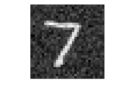
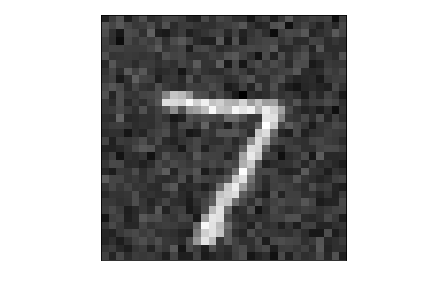
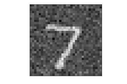
We further investigate influences on aleatoric uncertainty estimations by additive standard Gaussian noise of different levels. Here, a random sample of the standard Gaussian distribution is multiplied by a level and added to each pixel value. We test for and see that aleatoric uncertainty is independent of the added noise level (see Figure 3), i.e. aleatoric uncertainty is constant to six decimal places. Our intuition for this phenomenon is as follows: by normalizing the output of the Softplus function among one batch, of which all images have the same added level of noise, the aleatoric uncertainty captures the variability among the images in one batch - and not across batches with different levels of noise.


5 Conclusion
We propose a novel method how aleatoric and epistemic uncertainties can be estimated in Bayesian Cnns. We call this method Softplus normalization. Firstly, we discuss briefly the differences of a Bayes by Backprop based variational inference to the Dropout based approximation of Gal & Ghahramani [21]. Secondly, we derive the Softplus normalization uncertainty estimation method with previously published methods for these uncertainties. We evaluate our approach on three datasets (MNIST, CIFAR-10, CIFAR-100).
As a base, we show that Bayesian Cnns with variational inference achieve comparable results as those achieved by the same network architectures trained by frequentist inference, but include naturally a regularization effect and an uncertainty measure. Building on that, we examine how our proposed Softplus normalization method to estimate aleatoric and epistemic uncertainties is derived by previous work in this field, how it differs from those, and explain why it is more appropriate to use in computer vision than these previously proposed methods.
References
- [1] Kaiming He, Xiangyu Zhang, Shaoqing Ren, and Jian Sun. Deep residual learning for image recognition. In Proceedings of the IEEE conference on computer vision and pattern recognition, pages 770–778, 2016.
- [2] Karen Simonyan and Andrew Zisserman. Very deep convolutional networks for large-scale image recognition. arXiv preprint arXiv:1409.1556, 2014.
- [3] Alex Krizhevsky, Ilya Sutskever, and Geoffrey E Hinton. Imagenet classification with deep convolutional neural networks. In Advances in neural information processing systems, pages 1097–1105, 2012.
- [4] Alex Graves. Practical variational inference for neural networks. In Advances in Neural Information Processing Systems, pages 2348–2356, 2011.
- [5] Charles Blundell, Julien Cornebise, Koray Kavukcuoglu, and Daan Wierstra. Weight uncertainty in neural networks. arXiv preprint arXiv:1505.05424, 2015.
- [6] Yongchan Kwon, Joong-Ho Won, Beom Joon Kim, and Myunghee Cho Paik. Uncertainty quantification using bayesian neural networks in classification: Application to ischemic stroke lesion segmentation. 2018.
- [7] Zachary C Lipton, Jianfeng Gao, Lihong Li, Xiujun Li, Faisal Ahmed, and Li Deng. Efficient exploration for dialogue policy learning with bbq networks & replay buffer spiking. arXiv preprint arXiv:1608.05081, 2016.
- [8] Rein Houthooft, Xi Chen, Yan Duan, John Schulman, Filip De Turck, and Pieter Abbeel. Curiosity-driven exploration in deep reinforcement learning via bayesian neural networks. arXiv preprint arxiv.1605.09674, 2016.
- [9] Meire Fortunato, Charles Blundell, and Oriol Vinyals. Bayesian recurrent neural networks. arXiv preprint arXiv:1704.02798, 2017.
- [10] Kumar Shridhar, Felix Laumann, and Marcus Liwicki. A comprehensive guide to bayesian convolutional neural network with variational inference. CoRR, abs/1901.02731, 2019.
- [11] Kirill Neklyudov, Dmitry Molchanov, Arsenii Ashukha, and Dmitry Vetrov. Variance networks: When expectation does not meet your expectations. arXiv preprint arXiv:1803.03764, 2018.
- [12] Wray L Buntine and Andreas S Weigend. Bayesian back-propagation. Complex systems, 5(6):603–643, 1991.
- [13] Geoffrey E Hinton and Drew Van Camp. Keeping the neural networks simple by minimizing the description length of the weights. In Proceedings of the sixth annual conference on Computational learning theory, pages 5–13. ACM, 1993.
- [14] Sepp Hochreiter and Jürgen Schmidhuber. Simplifying neural nets by discovering flat minima. In Advances in neural information processing systems, pages 529–536, 1995.
- [15] John S Denker and Yann LeCu. Transforming neural-net output levels to probability distributions. In Advances in neural information processing systems, pages 853–859, 1991.
- [16] David JC MacKay. Probable networks and plausible predictions—a review of practical bayesian methods for supervised neural networks. Network: Computation in Neural Systems, 6(3):469–505, 1995.
- [17] Radford M Neal. Bayesian learning for neural networks, volume 118. Springer Science & Business Media, 2012.
- [18] Alex Graves. Stochastic backpropagation through mixture density distributions. arXiv preprint arXiv:1607.05690, 2016.
- [19] Nitish Srivastava, Geoffrey Hinton, Alex Krizhevsky, Ilya Sutskever, and Ruslan Salakhutdinov. Dropout: a simple way to prevent neural networks from overfitting. The Journal of Machine Learning Research, 15(1):1929–1958, 2014.
- [20] Sida Wang and Christopher Manning. Fast dropout training. In international conference on machine learning, pages 118–126, 2013.
- [21] Yarin Gal and Zoubin Ghahramani. Bayesian convolutional neural networks with bernoulli approximate variational inference. arXiv preprint arXiv:1506.02158, 2015.
- [22] Diederik P Kingma, Tim Salimans, and Max Welling. Variational dropout and the local reparameterization trick. In Advances in Neural Information Processing Systems, pages 2575–2583, 2015.
- [23] Christos Louizos and Max Welling. Multiplicative normalizing flows for variational bayesian neural networks. In Proceedings of the 34th International Conference on Machine Learning-Volume 70, pages 2218–2227. JMLR. org, 2017.
- [24] Lars Maaløe, Casper Kaae Sønderby, Søren Kaae Sønderby, and Ole Winther. Auxiliary deep generative models. arXiv preprint arXiv:1602.05473, 2016.
- [25] Chunyuan Li, Andrew Stevens, Changyou Chen, Yunchen Pu, Zhe Gan, and Lawrence Carin. Learning weight uncertainty with stochastic gradient mcmc for shape classification. In Proceedings of the IEEE Conference on Computer Vision and Pattern Recognition, pages 5666–5675, 2016.
- [26] Solomon Kullback and Richard A Leibler. On information and sufficiency. The annals of mathematical statistics, 22(1):79–86, 1951.
- [27] Radford M Neal and Geoffrey E Hinton. A view of the em algorithm that justifies incremental, sparse, and other variants. In Learning in graphical models, pages 355–368. Springer, 1998.
- [28] Jonathan S Yedidia, William T Freeman, and Yair Weiss. Constructing free-energy approximations and generalized belief propagation algorithms. IEEE Transactions on information theory, 51(7):2282–2312, 2005.
- [29] Karl Friston, Jérémie Mattout, Nelson Trujillo-Barreto, John Ashburner, and Will Penny. Variational free energy and the laplace approximation. Neuroimage, 34(1):220–234, 2007.
- [30] Diederik P Kingma and Jimmy Ba. Adam: A method for stochastic optimization. arXiv preprint arXiv:1412.6980, 2014.
- [31] Dmitry Molchanov, Arsenii Ashukha, and Dmitry Vetrov. Variational dropout sparsifies deep neural networks. arXiv preprint arXiv:1701.05369, 2017.
- [32] Armen Der Kiureghian and Ove Ditlevsen. Aleatory or epistemic? does it matter? Structural Safety, 31(2):105–112, 2009.
- [33] Alex Kendall and Yarin Gal. What uncertainties do we need in bayesian deep learning for computer vision? In Advances in neural information processing systems, pages 5574–5584, 2017.
- [34] Yann LeCun, Leon Bottou, Yoshua Bengio, and Patrick Haffner. Gradient-based learning applied to document recognition. Proceedings of the IEEE, 86(11):2278–2324, 1998.
- [35] Alex Krizhevsky and Geoffrey Hinton. Learning multiple layers of features from tiny images. Technical report, Citeseer, 2009.
6 Appendix
6.1 Experiment specifications
6.2 Model architectures
6.2.1 LeNet-5
| layer type | width | stride | padding | input shape | nonlinearity |
|---|---|---|---|---|---|
| convolution () | 6 | 1 | 0 | Softplus | |
| Mmax-pooling () | 2 | 0 | |||
| convolution () | 16 | 1 | 0 | Softplus | |
| max-pooling () | 2 | 0 | |||
| fully-connected | 120 | Softplus | |||
| fully-connected | 84 | Softplus | |||
| fully-connected | 10 | Softplus normalization |
6.2.2 AlexNet
| layer type | width | stride | padding | input shape | nonlinearity |
|---|---|---|---|---|---|
| convolution () | 64 | 4 | 5 | Softplus | |
| max-pooling () | 2 | 0 | |||
| convolution () | 192 | 1 | 2 | Softplus | |
| max-pooling () | 2 | 0 | |||
| convolution () | 384 | 1 | 1 | Softplus | |
| convolution () | 256 | 1 | 1 | Softplus | |
| convolution () | 128 | 1 | 1 | Softplus | |
| max-pooling () | 2 | 0 | |||
| fully-connected | 128 | Softplus normalization |
6.2.3 VGG
| layer type | width | stride | padding | input shape | nonlinearity |
|---|---|---|---|---|---|
| convolution () | 64 | 1 | 1 | Softplus | |
| convolution () | 64 | 1 | 1 | Softplus | |
| max-pooling () | 2 | 0 | |||
| convolution () | 128 | 1 | 1 | Softplus | |
| convolution () | 128 | 1 | 1 | Softplus | |
| max-pooling () | 2 | 0 | |||
| convolution () | 256 | 1 | 1 | Softplus | |
| convolution () | 256 | 1 | 1 | Softplus | |
| convolution () | 256 | 1 | 1 | Softplus | |
| max-pooling () | 2 | 0 | |||
| convolution () | 512 | 1 | 1 | Softplus | |
| convolution () | 512 | 1 | 1 | Softplus | |
| convolution () | 512 | 1 | 1 | Softplus | |
| max-pooling () | 2 | 0 | |||
| convolution () | 512 | 1 | 1 | Softplus | |
| convolution () | 512 | 1 | 1 | Softplus | |
| convolution () | 512 | 1 | 1 | Softplus | |
| max-pooling () | 2 | 0 | |||
| fully-connected | 512 | Softplus normalization |