oddsidemargin has been altered.
textheight has been altered.
marginparsep has been altered.
textwidth has been altered.
marginparwidth has been altered.
marginparpush has been altered.
The page layout violates the UAI style.
Please do not change the page layout, or include packages like geometry,
savetrees, or fullpage, which change it for you.
We’re not able to reliably undo arbitrary changes to the style. Please remove
the offending package(s), or layout-changing commands and try again.
BubbleRank: Safe Online Learning to Re-Rank via Implicit Click Feedback
Abstract
In this paper, we study the problem of safe online learning to re-rank, where user feedback is used to improve the quality of displayed lists. Learning to rank has traditionally been studied in two settings. In the offline setting, rankers are typically learned from relevance labels created by judges. This approach has generally become standard in industrial applications of ranking, such as search. However, this approach lacks exploration and thus is limited by the information content of the offline training data. In the online setting, an algorithm can experiment with lists and learn from feedback on them in a sequential fashion. Bandit algorithms are well-suited for this setting but they tend to learn user preferences from scratch, which results in a high initial cost of exploration. This poses an additional challenge of safe exploration in ranked lists. We propose , a bandit algorithm for safe re-ranking that combines the strengths of both the offline and online settings. The algorithm starts with an initial base list and improves it online by gradually exchanging higher-ranked less attractive items for lower-ranked more attractive items. We prove an upper bound on the -step regret of that degrades gracefully with the quality of the initial base list. Our theoretical findings are supported by extensive experiments on a large-scale real-world click dataset.
1 INTRODUCTION
Learning to rank (LTR) is an important problem in many application domains, such as information retrieval, ad placement, and recommender systems [23]. More generally, LTR arises in any situation where multiple items, such as web pages, are presented to users. It is particularly relevant when the diversity of users makes it hard to decide which item should be presented to a specific user [28, 37].
A traditional approach to LTR is offline learning of rankers from either relevance labels created by judges [26] or user interactions [13, 24]. Recent experimental results [38] shows that such rankers, even in a highly-optimized search engine, can be improved by online LTR with exploration. Exploration is the key component in multi-armed bandit algorithms [3]. Many such algorithms have been proposed recently for online LTR in specific user-behavior models [15, 17, 19], the so-called click models [6]. Compared to earlier online LTR algorithms [28], these click model-based algorithms gain in statistical efficiency while giving up on generality. Empirical results indicate that click model-based algorithms are likely to be beneficial in practice.
Yet, existing algorithms for online LTR in click models are impractical for at least three reasons. First, an actual model of user behavior is typically unknown. This problem was initially addressed by Zoghi et al. [39]. They showed that the list of items in the descending order of relevance is optimal in several click models and proposed for learning it. Then Lattimore et al. [20] built upon this work and proposed , which is the state-of-the-art online LTR algorithm. Second, these algorithms lack safety constraints and explore aggressively by placing potentially irrelevant items at high positions, which may significantly degrade user experience [34]. A third and related problem is that the algorithms are not well suited for so-called warm start scnearios [33], where the offline-trained production ranker already generates a good list, which only needs to be safely improved. Warm-starting an online LTR algorithm is challenging since existing posterior sampling algorithms, such as Thompson sampling [32], require item-level priors while only list-level priors are available practically.
We make the following contributions. First, motivated by the exploration scheme of Radlinski and Joachims [27], we propose a bandit algorithm for online LTR that addresses all three issues mentioned above. The proposed algorithm gradually improves upon an initial base list by exchanging higher-ranked less attractive items for lower-ranked more attractive items. The algorithm resembles bubble sort [8], and therefore we call it . Second, we prove an upper bound on the -step regret of . The bound reflects the behavior of : worse initial base lists lead to a higher regret. Third, we define our safety constraint, which is based on incorrectly-ordered item pairs in the ranked list, and prove that never violates this constraint with a high probability. Finally, we evaluate extensively on a large-scale real-world click dataset.
2 BACKGROUND
This section introduces our online learning problem. We first review click models [6] and then introduce a stochastic click bandit [39], a learning to rank framework for multiple click models.
The following notation is used in the rest of the paper. We denote by . For any sets and , we denote by the set of all vectors whose entries are indexed by and take values from . We use boldface letters to denote random variables.
2.1 CLICK MODELS
A click model is a model of how a user clicks on a list of documents. We refer to the documents as items and denote the universe of all items by . The user is presented a ranked list, an ordered list of documents out of . We denote this list by , where is the set of all -tuples with distinct items from . We denote by the item at position in ; and by the position of item in , if item is in .
Many click models are parameterized by item-dependent attraction probabilities , where is the attraction probability of item . We discuss the two most fundamental click models below.
In the cascade model (CM) [9], the user scans list from the first item to the last . If item is attractive, the user clicks on it and does not examine the remaining items. If item is not attractive, the user examines item . The first item is examined with probability one. Therefore, the expected number of clicks is equal to the probability of clicking on any item, and is , where is the examination probability of position in list .
In the position-based model (PBM) [29], the probability of clicking on an item depends on both its identity and position. Therefore, in addition to item-dependent attraction probabilities , the PBM is parameterized by position-dependent examination probabilities , where is the examination probability of position . The user interacts with list as follows. The user examines position with probability and then clicks on item at that position with probability . Therefore, the expected number of clicks on list is .
CM and PBM are similar models, because the probability of clicking factors into item and position dependent factors. Therefore, both in the CM and PBM, under the assumption that , the expected number of clicks is maximized by listing the most attractive items in descending order of their attraction. More precisely, the most clicked list is
| (1) |
when . Therefore, perhaps not surprisingly, the problem of learning the optimal list in both models can be viewed as the same problem, a stochastic click bandit [39].
2.2 STOCHASTIC CLICK BANDIT
An instance of a stochastic click bandit [39] is a tuple , where is the number of positions, is the number of items, is a distribution over binary attraction vectors , and is a distribution over binary examination matrices .
The learning agent interacts with the stochastic click bandit as follows. At time , it chooses a list , which depends on its history up to time , and then observes clicks on all positions in . A position is clicked if and only if it is examined and the item at that position is attractive. More specifically, for any ,
| (2) |
where and is the examination indicator of position in list at time ; and and is the attraction indicator of item at time . Both and are stochastic and drawn i.i.d. from .
The key assumption that allows learning in this model is that the attraction of any item is independent of the examination of its position. In particular, for any list and position ,
| (3) |
where and is the attraction probability of item ; and and is the examination probability of position in . Note that the above independence assumption is in expectation only. We do not require that the clicks are independent of the position or other displayed items.
The expected reward at time is the expected number of clicks at time . Based on our independence assumption, , where for any , , and . The learning agent maximizes the expected number of clicks in steps. This problem can be equivalently viewed as minimizing the expected cumulative regret in steps, which we define as
| (4) |
3 ONLINE LEARNING TO RE-RANK
Multi-stage ranking is widely used in production ranking systems [5, 14, 22], with the re-ranking stage at the very end [5]. In the re-ranking stage, a relatively small number of items, typically –, are re-ranked. One reason for re-ranking is that offline rankers are typically trained to minimize the average loss across a large number of queries. Therefore, they perform well on very frequent queries and poorly on infrequent queries. On moderately frequent queries, the so-called torso queries, their performance varies. As torso queries are sufficiently frequent, an online algorithm can be used to re-rank so as to optimize their value, such as the number of clicks [38].
We propose an online algorithm that addresses the above problem and adaptively re-ranks a list of items generated by a production ranker with the goal of placing more attractive items at higher positions. We study a non-contextual variant of the problem, where we re-rank a small number of items in a single query. Generalization across queries and items is an interesting direction for future work. We follow the setting in Section 2.2, except that . Despite these simplifying assumptions, our learning problem remains a challenge. In particular, the attraction of items is only observed through clicks in (2), which are affected by other items in the list.
3.1 ALGORITHM
Our algorithm is presented in Algorithm 1. The algorithm gradually improves upon an initial base list by “bubbling up” more attractive items. Therefore, we refer to it as . determines more attractive items by randomly exchanging neighboring items. If the lower-ranked item is found to be more attractive, the items are permanently exchanged and never randomly exchanged again. If the lower-ranked item is found to be less attractive, the items are never randomly exchanged again. We describe in detail below.
maintains a base list at each time . From the viewpoint of , this is the best list at time . The list is initialized by the initial base list (line 3). At time , permutes into a displayed list (lines 6–10). Two kinds of permutations are employed. If is odd and so , the items at positions and , and , and so on, are randomly exchanged. If is even and so , the items at positions and , and , and so on are randomly exchanged. The items are exchanged only if is uncertain regarding which item is more attractive (line 9).
The list is displayed and gets feedback (line 11). Then it updates its statistics (lines 12–19). For any exchanged items and , if item is clicked and item is not, the belief that is more attractive than , , increases; and the belief that is more attractive than , , decreases. The number of observations, and , increases. These statistics are updated only if one of the items is clicked (line 15), not both.
At the end of time , the base list is improved (lines 20–24). More specifically, if any lower-ranked item is found to be more attractive than its higher-ranked neighbor (line 23), the items are permanently exchanged in the next base list .
A notable property of is that it explores safely, since any item in the displayed list is at most one position away from its position in the base list . Moreover, any base list improves upon the initial base list , because it is obtained by bubbling up more attractive items with a high confidence. We make this notion of safety more precise in Section 4.2.
4 THEORETICAL ANALYSIS
In this section, we provide theoretical guarantees on the performance of , by bounding the -step regret in (4).
The content is organized as follows. In Section 4.1, we present our upper bound on the -step regret of , together with our assumptions. In Section 4.2, we prove that is safe. In Section 4.3, we discuss our theoretical results. The regret bound is proved in Section 4.4. Our technical lemmas are stated and proved in Appendix A.
4.1 REGRET BOUND
Before we present our result, we introduce our assumptions111Our assumptions are slightly weaker than those of Zoghi et al. [39]. For instance, Assumption A2 is on the probability of examination. Zoghi et al. [39] make this assumption on the realization of examination. and complexity metrics.
Assumption 1.
For any lists and positions such that :
-
A1.
, where is defined in (1);
-
A2.
;
-
A3.
;
-
A4.
If and differ only in that the items at positions and are exchanged, then ; and
-
A5.
.
The above assumptions hold in the CM. In the PBM, they hold when the examination probability decreases with the position.
Our assumptions can be interpreted as follows. Assumption A1 says that the list of items in the descending order of attraction probabilities is optimal. Assumption A2 says that the examination probability of any position depends only on the identities of higher-ranked items. Assumption A3 says that a higher position is at least as examined as a lower position. Assumption A4 says that a higher-ranked item is less attractive if and only if it increases the examination of a lower position. Assumption A5 says that any position is examined the least in the optimal list.
To simplify our exposition, we assume that . Let denote the maximum examination probability, denote the minimum examination probability, and
be the minimum gap. Then the -step regret of can be bounded as follows.
Theorem 1.
In any stochastic click bandit that satisfies 1, and for any , the expected -step regret of is bounded as
4.2 SAFETY
Let
| (5) |
be the set of incorrectly-ordered item pairs in list . Then our algorithm is safe in the following sense.
Lemma 2.
Let
| (6) |
be the incorrectly-ordered item pairs in the initial base list . Then the number of incorrectly-ordered item pairs in any displayed list is at most , that is holds uniformly over time with probability of at least .
Proof.
Our claim follows from two observations. First, by the design of , any displayed list contains at most item pairs that are ordered differently from its base list . Second, no base list contains more incorrectly-ordered item pairs than with a high probability. In particular, under event in Lemma 9, any change in the base list (line 24 of ) reduces the number of incorrectly-order item pairs by one. In Lemma 9, we prove that . ∎
4.3 DISCUSSION
Our upper bound on the -step regret of (Theorem 1) is for . This dependence is considered to be optimal in gap-dependent bounds. Our gap is the minimum difference in the attraction probabilities of items, and reflects the hardness of sorting the items by their attraction probabilities. This sorting problem is equivalent to the problem of learning . So, a gap like is expected, and is the same as that in Zoghi et al. [39].
Our regret bound is notable because it reflects two key characteristics of . First, the bound is linear in the number of incorrectly-ordered item pairs in the initial base list . This suggests that should have lower regret when initialized with a better list of items. We validate this dependence empirically in Section 5. In many domains, such lists exist and are produced by existing ranking policies. They only need to be safely improved.
Second, the bound is , where and are the maximum and minimum examination probabilities, respectively. In Section 5.4, we show that this dependence can be observed in problems where most attractive items are placed at infrequently examined positions. This limitation is intrinsic to , because attractive lower-ranked items cannot be placed at higher positions unless they are observed to be attractive at lower, potentially infrequently examined, positions.
The safety constraint of is stated in Lemma 2. For , as discussed above, becomes a rather safe algorithm, and is unlikely to display any list with more than incorrectly-ordered item pairs than the initial base list . More precisely, holds uniformly over time with probability of at least . This safety feature of is confirmed by our experiments in Section 5.3.
The above discussion assumes that the time horizon is known. However, in practice, this is not always possible. We can extend to the setting of an unknown time horizon by using the so-called doubling trick [4, Section 2.3]. Let be the estimated horizon. Then at time , is set to and is doubled. The statistics do not need to be reset.
is computationally efficient. The time complexity of is linear in the number of time steps and in each step operations are required.
In this paper, we focus on re-ranking. But can be extended to the full ranking problem as follows. Define and for all item pairs . For even (odd) at odd (even) time steps, select a random item below position that has not been shown to be worse than the item at position , and swap these items with probability . The item that is not displayed gets feedback . The rest of remains the same. This algorithm can be analyzed in the same way as .
4.4 PROOF OF THEOREM 1
In Lemma 9, we establish that there exists a favorable event that holds with probability , when all beliefs are at most from their respective means, uniformly for and . Since the maximum -step regret is , we get that
where . We bound next. For this, let
be the set of potentially randomized item pairs at time . Then, by Lemma 5 on event , which bounds the regret of list with the difference in the attraction probabilities of items , we have that
Now note that for any randomized at time ,
where is the expectation conditioned on the history up to time , . The inequality is from , and Assumptions A2 and A4. The above two inequalities yield
where the extra factor of two is because randomizes any pair of items at least once in any two consecutive steps. Moreover, for any on event ,
The first inequality is by Lemma 7, which establishes that the maximum difference in clicks of any randomized pair of items is bounded. After that, the better item is found and the pair of items is never randomized again. The last inequality is by and . Now we chain the above two inequalities and get that
Finally, let . Then, on event , . This follows from the design of (Lemma 6) and completes the proof. ∎
5 EXPERIMENTAL RESULTS
We conduct four experiments to evaluate . In Section 5.1, we describe our experimental setup. In Section 5.2, we report the regret of compared algorithms, which measures the rate of convergence to the optimal list in hindsight. In Section 5.3, we validate the safety of . In Section 5.4, we validate the tightness of the regret bound in Theorem 1. Due to space limitations, we report the Normalized Discounted Cumulative Gain (NDCG) of compared algorithms, which measures the quality of displayed lists, in Appendix B.
5.1 EXPERIMENTAL SETUP
We evaluate on the Yandex click dataset.222https://academy.yandex.ru/events/data_analysis/relpred2011 The dataset contains user search sessions from the log of the Yandex search engine. It is the largest publicly available dataset containing user clicks, with more than million search sessions. Each session contains at least one search query together with ranked items.
We preprocess the dataset as in [39]. In particular, we randomly select frequent search queries, and then learn the parameters of three click models using the PyClick333https://github.com/markovi/PyClick package: CM and PBM, described in Section 2.1, as well as the dependent click model (DCM) [10].
The DCM is an extension of the CM [9] where each position is associated with an abandonment probability . When the user clicks on an item at position , the user stops scanning the list with probability . Therefore, the DCM can model multiple clicks. Following the work in [15], we incorporate abandonment into our definition of reward for DCM and define it as the number of abandonment clicks. The abandonment click is a click after which a user stops browsing the list, and each time step contains at most one abandonment click. So, the expected reward for DCM equals the probability of abandonment clicks, which is computed as follows:
is the examination probability of position in list . A high reward means a user stops the search session because of clicking on an item with high attraction probability.
The learned CM, DCM, and PBM are used to simulate user click feedback. We experiment with multiple click models to show the robustness of to multiple models of user feedback.
For each query, we choose items. The number of positions is equal to the number of items, . The objective of our re-ranking problem is to place most attractive items in the descending order of their attractiveness at the highest positions, as in [39]. The performance of and our baselines is also measured only at the top positions.
is compared to three baselines [17], [39], and [20]. The former is near optimal in the CM [17], but can have linear regret in other click models. Note that linear regret arises when erroneously converges to a suboptimal ranked list. and can learn the optimal list in a wide range of click models, including the CM, DCM, and PBM. However, they can perform poorly in early stages of learning because they randomly shuffles displayed lists to average out the position bias. All experiments are run for million steps, after which at least two algorithms converge to the optimal ranked list.
In the Yandex dataset, each query is associated with many different ranked lists, due to the presence of various personalization features of the production ranker. We take the most frequent ranked list for each query as the initial base list in , since we assume that the most frequent ranked list is what the production ranker would produce in the absence of any personalization. We also compare to a production baseline, called , where the initial list is applied for steps.
5.2 RESULTS WITH REGRET
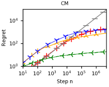
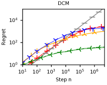
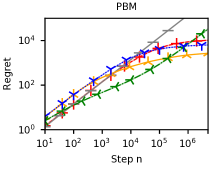
In the first experiment, we compare to , , and in the CM, DCM, and PBM of all queries. Among them, is the state-of-the-art online LTR algorithm in multiple click models. We evaluate these algorithms by their cumulative regret, which is defined in (4), at the top positions. The regret, a measure of convergence, is a widely-used metric in the bandit literature [3, 15, 17, 39]. In the CM and PBM, the regret is the cumulative loss in clicks when a sequence of learned lists is compared to the optimal list in hindsight. In the DCM, the regret is the cumulative loss in abandonment clicks. We also report the regret of .
Our results are reported in Figure 1. We observe that the regret of grows linearly with time , which means that it is not optimal on average. learns quickly in both the CM and DCM, but has linear regret in the PBM. This is expected since is designed for the CM, and the DCM is an extension of the CM. As for the PBM, which is beyond the modeling assumptions of , there is no guarantee on the performance of . , , and can learn in all three click models. Compared to and , has a higher regret in million steps. However, in earlier steps, has a lower regret than and , as it takes advantage of the initial base list . In general, these results show that converges to the optimal list slower than and . This is expected because is designed to be a safe algorithm, and only learns better lists by exchanging neighboring items in the base list.
5.3 SAFETY RESULTS
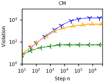
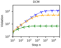
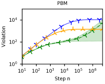
In the previous experiment, we show that does not learn as fast as , , and because it operates under the additional safety constraint in Lemma 2. The constraint is that is unlikely to display any list with more than incorrectly-ordered item pairs than the initial base list . More precisely, holds uniformly over time with probability of at least for (Section 4.3), where is defined in (5). In the second experiment, we answer the question how often do , , , and violate this constraint empirically. We define the safety constraint violation in steps as
| (7) |
where is the displayed list at time .
We report the -step safety constraint violation of , , and in Figure 2. We do not include results of since never violates the constraint in our experiments. We observe that the safety constraint violations of in the first steps are , , and in the CM, DCM, and PBM, respectively. Translating this to a search scenario, may show unsafe results, which are significantly worse than the initial base list , and may hurt user experience, more than of search sessions in the first steps. Even worse, the violations of grow linearly with time in the PBM. The safety issues of , and are more severe than that of . More precisely, the violations of in the first steps are , , and in the CM, DCM, and PBM, respectively. And the violations of are , , and in the CM, DCM, and PBM, respectively. Note that the performance of is close to that of in the first steps since they both require the ranked lists to be randomly shuffled during the initial stages. Thus, , and would frequently hurt the user experience during the early stages of learning.
To conclude, learns without violating its safety constraint, while , , and violate the constraint frequently. Together with results in Section 5.2, is a safe algorithm but, to satisfy the safety constraint, it compromises the performance and learns slower than and . In Appendix B, we compare to baselines in NDCG and show that converges to the optimal lists in hindsight.
5.4 SANITY CHECK ON THE REGRET BOUND
We prove an upper bound on the -step regret of in Theorem 1. In comparison to the upper bounds of [17] and [39], we have two new problem-specific constants: and . In this section, we show that these constants are intrinsic to the behavior of .
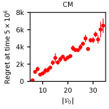
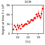
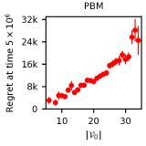
We first study how the number of incorrectly-ordered item pairs in the initial base list , , impacts the regret of . We choose random initial base lists in each of our queries and plot the regret of as a function of . Our results are shown in Figure 3. We observe that the regret of is linear in in the CM, DCM, and PBM. This is the same dependence as in our regret bound (Theorem 1).
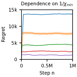
We then study the impact of the minimum examination probability on the regret of . We experiment with a synthetic PBM with items, which is parameterized by and for . The most attractive item is placed at the last position in , . Since this position is examined with probability , we expect the regret to double when increases by one. We experiment with in Figure 3 and observe this trend in million steps. This confirms that the dependence on in Theorem 1 is generally unavoidable.
6 RELATED WORK
Online LTR via click feedback has been mainly studied in two approaches: under specific click models [7, 15, 17, 18, 19, 40]; or without a particular assumption on click models [20, 28, 30, 39]. Algorithms from the first group efficiently learn optimal rankings in the their considered click models but do not have guarantees beyond their specific click models. Algorithms from the second group, on the other hand, learn the optimal rankings in a broader class of click models. [20] is the state-of-the-art of the second group, which has the regret of in our re-ranking setup, that is . also belongs to the second group and the regret of is comparable to that of given a good initial list, when . However, unlike , and all the previous algorithms do not consider safety. They explore aggressively in the initial steps and may display irrelevant items at high positions, which may then hurt user experiences [34].
Our safety problem is related to the warm start problem [31]. Contextual bandits [1, 21, 25] deal with a broader class of models than we do and are used to address the warm start problem. But they are limited to small action sets, and thus unsuitable for the ranking setup that we consider in this paper.
The warm start LTR has been studied in multiple papers [11, 33, 36], where the goal is to use an online algorithm to fine tune the results generated by an offline-trained ranker. In these papers, different methods for learning prior distributions of Thompson sampling based online LTR algorithms from offline datasets have been proposed. However, these methods have the following drawbacks. First, the offline data may not well align with user preferences [38], which may result in a biased prior assumption. Second, grid search with online A/B tests may alleviate this and find a proper prior assumption [33], but the online A/B test requires additional costs in terms of user experience. Third, there is no safety constraint in these methods. Even with carefully picked priors, they may recommend irrelevant items to users, e.g., new items with little prior knowledge. In contrast, starts from the production ranked list and learns under the safety constraint. Thus, gets rid of these drawbacks.
Another related line of work are conservative bandits [16, 35]. In conservative bandits, the learned policy is safe in the sense that its expected cumulative reward is at least fraction of that of the baseline policy with high probability. This notion of safety is less stringent than that in our work (Section 4.2). In particular, our notion of safety is per-step, in the sense that any displayed list is only slightly worse than the initial base list with a high probability. We do not compare to conservative bandits in our experiments because existing algorithms for conservative bandits require the action space to be small. The actions in our problem are ranked lists, and their number is exponential in .
7 CONCLUSIONS
In this paper, we fill a gap in the LTR literature by proposing , a re-ranking algorithm that gradually improves an initial base list, which we assume to be provided by an offline LTR approach. The improvements are learned from small perturbations of base lists, which are unlikely to degrade the user experience greatly. We prove a gap-dependent upper bound on the regret of and evaluate it on a large-scale click dataset from a commercial search engine.
We leave open several questions of interest. For instance, our paper studies in the setting of re-ranking. Although we explain an approach of extending to the general ranking setup in Section 4.3, we expect further experiments to validate this approach. Our general topic of interest are exploration schemes that are more conservative than those of existing online LTR methods. Existing methods are not very practical because they can explore highly irrelevant items at frequently examined positions.
ACKNOWLEDGMENTS
We thank our reviewers for helpful feedback and suggestions. This research was supported by Ahold Delhaize, the Association of Universities in the Netherlands (VSNU), the Innovation Center for Artificial Intelligence (ICAI), and the Netherlands Organisation for Scientific Research (NWO) under project nr. 612.001.551. All content represents the opinion of the authors, which is not necessarily shared or endorsed by their respective employers and/or sponsors.
References
- Agarwal et al. [2014] A. Agarwal, D. Hsu, S. Kale, J. Langford, L. Li, and R. Schapire. Taming the monster: A fast and simple algorithm for contextual bandits. In ICML, pages II–1638–II–1646, 2014.
- Allan et al. [2017] J. Allan, D. Harman, E. Kanoulas, D. Li, C. Van Gysel, and E. Voorhees. TREC 2017 common core track overview. TREC, 2017.
- Auer et al. [2002] P. Auer, N. Cesa-Bianchi, and P. Fischer. Finite-time analysis of the multiarmed bandit problem. Machine Learning, 47:235–256, 2002.
- Cesa-Bianchi and Lugosi [2006] N. Cesa-Bianchi and G. Lugosi. Prediction, Learning, and Games. Cambridge University Press, 2006.
- Chen et al. [2017] R.-C. Chen, L. Gallagher, R. Blanco, and J. S. Culpepper. Efficient cost-aware cascade ranking in multi-stage retrieval. In SIGIR, pages 445–454, 2017.
- Chuklin et al. [2015] A. Chuklin, I. Markov, and M. de Rijke. Click Models for Web Search. Morgan & Claypool, 2015.
- Combes et al. [2015] R. Combes, S. Magureanu, A. Proutiere, and C. Laroche. Learning to rank: Regret lower bounds and efficient algorithms. In SIGMETRICS, pages 231–244, 2015.
- Cormen et al. [2009] T. H. Cormen, C. E. Leiserson, R. L. Rivest, and C. Stein. Introduction to Algorithms, 3rd Edition. MIT Press, 2009.
- Craswell et al. [2008] N. Craswell, O. Zoeter, M. Taylor, and B. Ramsey. An experimental comparison of click position-bias models. In WSDM, pages 87–94, 2008.
- Guo et al. [2009] F. Guo, C. Liu, and Y. M. Wang. Efficient multiple-click models in web search. In WSDM, pages 124–131, 2009.
- Hofmann et al. [2013] K. Hofmann, A. Schuth, S. Whiteson, and M. de Rijke. Reusing historical interaction data for faster online learning to rank for ir. In WSDM, 2013.
- Järvelin and Kekäläinen [2002] K. Järvelin and J. Kekäläinen. Cumulated gain-based evaluation of IR techniques. ACM Trans. Inf. Syst., 20(4):422–446, 2002.
- Joachims [2002] T. Joachims. Optimizing search engines using clickthrough data. SIGKDD, pages 133–142, 2002.
- Karmaker Santu et al. [2017] S. K. Karmaker Santu, P. Sondhi, and C. Zhai. On application of learning to rank for e-commerce search. In SIGIR, pages 475–484, New York, NY, USA, 2017.
- Katariya et al. [2016] S. Katariya, B. Kveton, C. Szepesvari, and Z. Wen. DCM bandits: Learning to rank with multiple clicks. In ICML, pages 1215–1224, 2016.
- Kazerouni et al. [2017] A. Kazerouni, M. Ghavamzadeh, Y. Abbasi, and B. Van Roy. Conservative contextual linear bandits. In NIPS, pages 3913–3922, 2017.
- Kveton et al. [2015a] B. Kveton, C. Szepesvari, Z. Wen, and A. Ashkan. Cascading bandits: Learning to rank in the cascade model. In ICML-15, pages 767–776, 2015a.
- Kveton et al. [2015b] B. Kveton, Z. Wen, A. Ashkan, and C. Szepesvari. Combinatorial cascading bandits. In NIPS, pages 1450–1458, 2015b.
- Lagrée et al. [2016] P. Lagrée, C. Vernade, and O. Cappe. Multiple-play bandits in the position-based model. In NIPS, pages 1605–1613, 2016.
- Lattimore et al. [2018] T. Lattimore, B. Kveton, S. Li, and C. Szepesvari. Toprank: A practical algorithm for online stochastic ranking. In NIPS, pages 3945–3954, 2018.
- Li et al. [2010] L. Li, W. Chu, J. Langford, and R. E. Schapire. A contextual-bandit approach to personalized news article recommendation. In WWW, pages 661–670, 2010.
- Liu et al. [2017] S. Liu, F. Xiao, W. Ou, and L. Si. Cascade ranking for operational e-commerce search. arXiv preprint arXiv:1706.02093, 2017.
- Liu [2009] T.-Y. Liu. Learning to rank for information retrieval. Foundations and Trends in Information Retrieval, 3(3):225–331, 2009.
- McMahan et al. [2013] H. B. McMahan, G. Holt, D. Sculley, M. Young, D. Ebner, J. Grady, L. Nie, T. Phillips, E. Davydov, D. Golovin, et al. Ad click prediction: a view from the trenches. In SIGKDD, pages 1222–1230, 2013.
- Moon et al. [2010] T. Moon, L. Li, W. Chu, C. Liao, Z. Zheng, and Y. Chang. Online learning for recency search ranking using real-time user feedback. In CIKM, pages 1501–1504, 2010.
- Qin et al. [2010] T. Qin, T.-Y. Liu, J. Xu, and H. Li. Letor: A benchmark collection for research on learning to rank for information retrieval. Information Retrieval, 13(4):346–374, 2010.
- Radlinski and Joachims [2006] F. Radlinski and T. Joachims. Minimally invasive randomization for collecting unbiased preferences from clickthrough logs. In AAAI, pages 1406–1412, 2006.
- Radlinski et al. [2008] F. Radlinski, R. Kleinberg, and T. Joachims. Learning diverse rankings with multi-armed bandits. In ICML, pages 784–791, 2008.
- Richardson et al. [2007] M. Richardson, E. Dominowska, and R. Ragno. Predicting clicks: Estimating the click-through rate for new ads. In WWW, pages 521–530, 2007.
- Slivkins et al. [2013] A. Slivkins, F. Radlinski, and S. Gollapudi. Ranked bandits in metric spaces: Learning diverse rankings over large document collections. Journal of Machine Learning Research, 14(1):399–436, 2013.
- Strehl et al. [2010] A. Strehl, J. Langford, L. Li, and S. M. Kakade. Learning from logged implicit exploration data. In NIPS, pages 2217–2225, 2010.
- Thompson [1933] W. R. Thompson. On the likelihood that one unknown probability exceeds another in view of the evidence of two samples. Biometrika, 25:285–294, 1933.
- Vorobev et al. [2015] A. Vorobev, D. Lefortier, G. Gusev, and P. Serdyukov. Gathering additional feedback on search results by multi-armed bandits with respect to production ranking. In WWW, pages 1177–1187, 2015.
- Wang et al. [2018] X. Wang, N. Golbandi, M. Bendersky, D. Metzler, and M. Najork. Position bias estimation for unbiased learning to rank in personal search. In WSDM, pages 610–618, 2018.
- Wu et al. [2016] Y. Wu, R. Shariff, T. Lattimore, and C. Szepesvári. Conservative bandits. In ICML, pages 1254–1262, 2016.
- Yan et al. [2018] Y. Yan, Z. Liu, M. Zhao, W. Guo, W. P. Yan, and Y. Bao. A practical deep online ranking system in e-commerce recommendation. In ECML PKDD, pages 186–201, 2018.
- Yue and Guestrin [2011] Y. Yue and C. Guestrin. Linear submodular bandits and their application to diversified retrieval. In NIPS, pages 2483–2491, 2011.
- Zoghi et al. [2016] M. Zoghi, T. Tunys, L. Li, D. Jose, J. Chen, C. M. Chin, and M. de Rijke. Click-based hot fixes for underperforming torso queries. In ACM SIGIR, pages 195–204. ACM, 2016.
- Zoghi et al. [2017] M. Zoghi, T. Tunys, M. Ghavamzadeh, B. Kveton, C. Szepesvari, and Z. Wen. Online learning to rank in stochastic click models. In ICML, pages 4199–4208, 2017.
- Zong et al. [2016] S. Zong, H. Ni, K. Sung, N. R. Ke, Z. Wen, and B. Kveton. Cascading bandits for large-scale recommendation problems. In UAI, pages 835–844, 2016.
Appendix A LEMMAS
Lemma 3.
Let be any list over . Let
| (8) |
be the attraction gap of list . Then the expected regret of is bounded as
Proof.
Fix position . Then
where the first inequality follows from the fact that the examination probability of any position is the lowest in the optimal list (Assumption A5) and the second inequality follows from the definition of . In the rest of the proof, we bound . We consider three cases. First, let . Then and can be trivially bounded by . Second, let and , where is the position of item in list . Then
From the definition of , this quantity is bounded from above by . Finally, let and . This implies that there exists an item at a lower position than , , such that . Then
From the definition of , this quantity is bounded from above by . This concludes the proof. ∎
Lemma 4.
Proof.
Fix list and position . Let be items at positions in . If , let ; and if , let . We consider two cases.
First, suppose that the permutation at time is such that and could be exchanged. Then
holds on event by the design of . More specifically, implies that .
Second, suppose that the permutation at time is such that and could be exchanged, and could be exchanged, or both. Then
holds by the same argument as in the first case. Also note that
holds on event by the design of . Therefore, for any position in both above cases,
Now we sum over all positions and note that each pair of and appears on the right-hand side at most three times, in any list . This concludes our proof. ∎
Proof.
From the design of , . The set of randomized item pairs grows only if the base list in changes. When this happens, the number of incorrectly-ordered item pairs decreases by one, on event , and the set of randomized item pairs increases by at most two pairs. This event occurs at most times. This concludes our proof. ∎
Lemma 7.
Proof.
To simplify notation, let and . The proof has two parts. First, suppose that holds at all times . Then from this assumption and on event in Lemma 9,
This implies that
at any time , and in turn that
at any time . Our claim follows from setting .
Now suppose that does not hold at all times . Let be the first time when . Then from the definition of and on event in Lemma 9,
where the last inequality holds for any . This implies that
and in turn that
Now note that for any , from the design of . This concludes our proof. ∎
For some -measurable event , let be the conditional probability of given history . Let the corresponding conditional expectation operator be . Note that is -measurable.
Lemma 8.
Let be any items at consecutive positions in and
Then, on the event that and are subject to randomization at time ,
when , and when .
Proof.
The first claim is proved as follows. From the definition of expectation and ,
where the last equality is a consequence of and that .
Let and denote the average examination probabilities of the positions with items and , respectively, in ; and consider the event that and are subject to randomization at time . By Assumption A2, the values of and do not depend on the randomization of other parts of , only on the positions of and . Then ; from and Assumption A4. Based on this fact, is bounded from below as
where the inequality is from . Moreover, is bounded from above as
where the first inequality is from inequalities and , and the last inequality is from .
Finally, we chain all above inequalities and get our first claim. The second claim follows from the observation that . ∎
Lemma 9.
Let and . Let
Let and be the complement of . Then .
Proof.
First, we bound . Fix , , and . Let be the time of observing item pair for the -th time, for . Let . Since is fixed, note that if for some . Let and
for . Then is a martingale, because
where the last equality follows from the definition of . Now we apply the Azuma-Hoeffding inequality and get that
Moreover, from the definitions of and , and by Lemma 8, we have that
The above inequality holds for any , and therefore also in expectation over . From the definition of and the union bound, we have .
The claim that is proved similarly, except that we use . From the definition of and the union bound,
This completes our proof. ∎
Appendix B RESULTS WITH NDCG
In this section, we report the NDCG of compared algorithms, which measures the quality of displayed lists. Since fails in the PBM and we focus on learning from all types of click feedback, we leave out from this section.
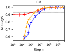
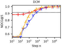
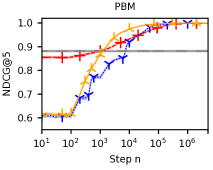
In the first two experiments, we evaluate algorithms by their regret in (4) and safety constraint violation in (7). Neither of these metrics measure the quality of ranked lists directly. In this experiment, we report the per-step NDCG@ of , , , and (Figure 4), which directly measures the quality of ranked lists and is widely used in the LTR literature [12, 2]. Since the Yandex dataset does not contain relevance scores for all query-item pairs, we take the attraction probability of the item in its learned click model as a proxy to its relevance score. This substitution is natural since our goal is to rank items in the descending order of their attraction probabilities [6]. We compute the NDCG@ of a ranked list as
where is the optimal list and is the attraction probability of the -th item in list . This is a standard evaluation metric, and is used in TREC evaluation benchmarks [2], for instance. It measures the discounted gain over the attraction probabilities of the highest ranked items in list , which is normalized by the DCG@ of .
In Figure 4, we observe that has good NDCG@ scores in all click models. Yet there is still room for improvement. , , and have similar NDCG@ scores after million steps. But starts with NDCG@ close to that of , while and start with lists with very low NDCG@.
These results validate our earlier findings. As in Section 5.2, we observe that converges to the optimal list in hindsight, since its NDCG@ approaches . As in Section 5.3, we observe that is safe, since its NDCG@ is never much worse than that of .
