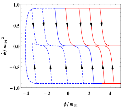
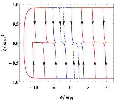
Preinflationary dynamics of Ξ±βˆ’limit-from𝛼\alpha-attractor in loop quantum cosmology

M. Shahalam1 111E-mail address: shahalam@zjut.edu.cn    M. Sami2 222 E-mail address: samijamia@gmail.com    Anzhong Wang1,3 333E-mail address: Anzhong__\_Wang@baylor.edu 1Institute for Advanced Physics &\& Mathematics, Zhejiang University of Technology, Hangzhou, 310032, China
2Centre for Theoretical Physics, Jamia Millia Islamia, New Delhi, 110025, India
3GCAP-CASPER, Department of Physics, Baylor University, Waco, TX, 76798-7316, USA
Abstract

We systematically study the preinflationary dynamics of the spatially flat Friedmann-Lemaitre-Robertson-Walker universe filled with a single scalar field that has the generalized Ξ±βˆ’limit-from𝛼\alpha-attractor potentials, in the framework of loop quantum cosmology, in which the big bang singularity is replaced generically by a non-singular quantum bounce due to purely quantum geometric effects. The evolution can be divided into two different classes, one is dominated initially (at the quantum bounce) by the kinetic energy of the scalar field, and one is not. In both cases, we identify numerically the physically viable initial conditions that lead to not only a slow-roll inflationary phase, but also enough e𝑒e-folds to be consistent with observations, and find that the output of such a viable slow-roll inflationary phase is generic. In addition, we also show that in the case when the evolution of the universe is dominated initially by the kinetic energy of the scalar field (except for a very small set in the phase space), the evolution before reheating is aways divided into three different phases: bouncing, transition and slow-roll inflation. This universal feature does not depend on the initial conditions of the system nor on the specific potentials of the scalar field, as long as it is dominated initially by the kinetic energy of the scalar field at the bounce. Moreover, we carry out phase space analyses for the models under consideration and compare our results with the power-law and Starobinsky potentials.

I Introduction

In the early 1980’s, the cosmic inflation stood out as a popular paradigm for resolving various problems in the standard model of cosmology, such as the horizon and flatness, etc. It also explains the origin of inhomogeneities that are observed in the cosmic microwave background and the formation of the large scale structure of the universe guth1981 . During the last three decades, a wide range of inflationary models have been proposed, including conformal attractors conformal , Ξ±βˆ’limit-from𝛼\alpha-attractors alpha ; alpha1 ; alpha2 ; alpha3 ; alpha4 , Starobinsky and the chaotic inflation in supergravity, which is known as Goncharov and Linde (GL) model staro1980 ; staro1 ; staro2 ; staro3 ; staro4 ; GL . These models provide very similar cosmological predictions with respect to the significant differences in their potentials, and have an excellent fit with the current observations. According to Planck 2015 results Planck2015 , in the case of a single field inflation, the potentials of Ξ±βˆ’limit-from𝛼\alpha-attractors and Starobinsky are consistent with the observations, while the quadratic potential is not equally favorable.

Despite the triumph of the standard inflationary models, which are based on the classical theory of general relativity (GR), their past is inadequate due to the existence of a big bang singularity. All scalar field models of inflation suffer from this initial and inevitable singularity borde1994 ; borde2003 . Clearly, with this it is difficult to know when and how to set the initial conditions. Moreover, to be consistent with the current observations, the universe should have expanded at least 60 e𝑒e-folds during the inflation. Meanwhile, in a large class of inflationary models, it is often more than 70 e𝑒e-folds martin2014 . However, in these models the size of the current universe is smaller than the Planck at the onset of inflation. Consequently, the semi-classical treatments are questionable during inflation. This is the so-called trans-Planckian problem martin2001 ; berger2013 .

To address the above issues, in this paper we shall study the preinflationary dynamics of the generalized Ξ±βˆ’limit-from𝛼\alpha-attractor model in the context of loop quantum cosmology (LQC), in which the big bang singularity is generically replaced by a quantum bounce agullo2013a ; agullo2013b ; agullo2015 ; ashtekar2011 ; ashtekar2015 ; barrau2016 , and investigate whether following the quantum bounce a desired slow-roll inflation generically exists or not ashtekar2010 ; psingh2006 ; zhang2007 ; chen2015 ; bolliet2015 ; schander2016 ; bolliet2016 ; Bonga2016 ; Mielczareka .

In the literature, there are mainly two distinct approaches for the preinflationary universe, the dressed metric agullo2013b ; metrica ; metricb ; metricc and the deformed algebra algebraa ; algebrab ; algebrac ; algebrad ; algebrae ; algebraf . Although both approaches give rise to the same set of dynamical equations in the case of the background evolution of the universe, their perturbations are different bolliet2016 . The corresponding non-Gaussianities were also studied both numerically agullo15 ; ABS17 and analytically ZWKCS18 recently, and found that it is consistent with current observations.

However, in this paper since we are mainly concerned with the background evolution of the universe, the results to be presented in this work will be valid to both approaches. Keeping this in mind, we shall compare our results with the power-law and Starobinsky potentials obtained in psingh2006 ; chen2015 ; Bonga2016 ; alam2017 ; Tao2017a ; Tao2017b . In particular, we shall show that, when the kinetic energy of the inflaton initially dominates at the bounce (except for a very small set in the phase space), the evolution of the universe before reheating can be divided universally into three different phases alam2017 ; Tao2017a ; Tao2017b : bouncing, transition and slow-roll inflation. During these phases, the evolutions of both background and linear perturbations of the universe are all known analytically Tao2017a ; Tao2017b . In the small exceptional region of the phase space, we find that the potential energy first evolutes almost as a constant in the bouncing phase, but oscillating afterward, in contrast to the rest of regions in which the kinetic energy of the inflaton dominates the evolution of the universe at the quantum bounce. As a result, in this exceptional region, a slow-roll inflation is not resulted.

The rest of the paper is organized as follows. In Sec. II, we briefly discuss the basic equations of the background evolution of the universe in the framework of LQC. In Sec. III, we examine the generalized Ξ±βˆ’limit-from𝛼\alpha-attractor model, and shall divide it into three models, namely T𝑇T, E𝐸E and Ξ±βˆ’limit-from𝛼\alpha-attractor with n=2𝑛2n=2 in the sub-sections III.1, III.2 and III.3, respectively. These sub-sections are devoted to the detailed analysis of the background evolution in the framework of the positive inflaton velocity (PIV, Ο•Λ™>0Λ™italic-Ο•0\dot{\phi}>0) and negative inflaton velocity (NIV, Ο•Λ™<0Λ™italic-Ο•0\dot{\phi}<0), and also in the form of kinetic energy dominated (KED) and potential energy dominated (PED) cases at the bounce. The phase portraits for the models under consideration are presented in Sec. IV. In Sec. V, we compare our results with the ones obtained previously for the power-law and Starobinsky potentials. Our main conclusions are summarized in Sec. VI.

Before turning to the next section, it is interesting to note that pre-inflationary universe has been also studied recently in the framework of loop quantum gravity (LQG) yang2009 ; DL17 ; adlp ; lsw2018a ; lsw2018b ; agullo18 by using Thiemann’s quantization scheme for the Lorentz part of the Hamiltonian thiemann , and among other things, it was shown that the resolution of the big bang singularity (replaced by a quantum bounce) is robust, although the details near the bounce depend on the ways to regularize the Hamiltonian lsw2018a ; lsw2018b . When the kinetic energy of the inflaton dominates at the bounce, the evolution of the universe before reheating can be also divided universally into three different phases, bouncing, transition and slow-roll inflation lsw2018a ; lsw2018b . During these phases, the evolution of the background of the universe is also known analytically Tao2017a ; Tao2017b .

We would also like to note that recently inflation with different potentials have been studied in Einstein’s theory of gravity and string-inspired models HISY ; BG15 ; sahni18 ; SW08 ; nozari , and various interesting results were obtained. In addition, in the framework of quantum reduced loop gravity (QRLG), its Hamiltonian (HQ​R​L​Gsubscript𝐻𝑄𝑅𝐿𝐺H_{QRLG}) is almost identical to the Hamiltonian of LQC (HL​Q​Csubscript𝐻𝐿𝑄𝐢H_{LQC}), except for a leading term QRLG1 ; QRLG2 . If this term is zero, then HQ​R​L​Gsubscript𝐻𝑄𝑅𝐿𝐺H_{QRLG} exactly coincides with HL​Q​Csubscript𝐻𝐿𝑄𝐢H_{LQC}. Similar to LQC, bounce occurs in QRLG. If we use the modified Friedmann equation of QRLG, then we can also obtain three different phases, bouncing, transition and the slow-roll inflation. However, the background dynamics would not be exactly the same as in LQC due to the dependence on the parameters of QRLG. Yet, the modified Friedmann equation of group field theory (GFT) is also almost the same as in LQC, except with the last term of energy Ej​0subscript𝐸𝑗0E_{j0} GFT1 ; GFT2 , The geometric interpretation of Ej​0subscript𝐸𝑗0E_{j0} is not transparent, but its effect on the dynamics is as following: (a) For Ej​0=0subscript𝐸𝑗00E_{j0}=0, the effective dynamics is same as in LQC. (b) For Ej​0>0subscript𝐸𝑗00E_{j0}>0, the bounce will take place at a higher space-time curvature. (c) For Ej​0<0subscript𝐸𝑗00E_{j0}<0, the bounce will occur at a lower space-time curvature.

The issue of estimating the duration of the slow-roll inflation with effective isotropic, anisotropic and Bianch I Universe in LQC have been investigated in LQC1 ; LQC2 ; LQC3 , in which it was found that the probability distribution function during the slow-roll inflation is peaked at the values of e-folds which are consistent with observations. Moreover, the duration of the slow-roll inflation does not depend crucially on the modified background evolution LQC4 . A new related study for the probability of inflation has been discussed in LQC5 , in which the existence of the quantum bounce affects the probability of inflation.
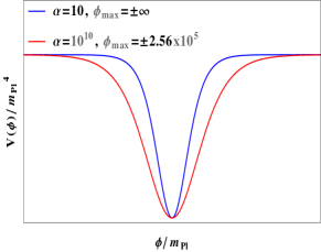
Refer to caption Refer to caption
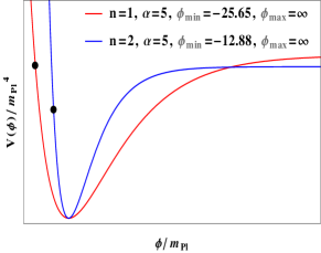
Figure 1: Left panel shows the evolution of the Tβˆ’m​o​d​e​lπ‘‡π‘šπ‘œπ‘‘π‘’π‘™T-model potential (16) for Ξ±=10​mP​l2𝛼10superscriptsubscriptπ‘šπ‘ƒπ‘™2\alpha=10m_{Pl}^{2} and 1010​mP​l2superscript1010superscriptsubscriptπ‘šπ‘ƒπ‘™210^{10}m_{Pl}^{2}. This potential is symmetric about Ο•=0italic-Ο•0\phi=0, and bounded by V​(Ο•)≀α​c2𝑉italic-ϕ𝛼superscript𝑐2V(\phi)\leq\alpha c^{2} (above, as Ο•β†’Β±βˆžβ†’italic-Ο•plus-or-minus\phi\rightarrow\pm\infty) and V​(Ο•)β‰₯0𝑉italic-Ο•0V(\phi)\geq 0 (below). In LQC, maximum energy density is ρcsubscriptπœŒπ‘\rho_{c} that constrains Ο•m​a​xsubscriptitalic-Ο•π‘šπ‘Žπ‘₯\phi_{max}, see Eq.(26). Therefore, ρ≀ρc𝜌subscriptπœŒπ‘\rho\leq\rho_{c} at the bounce. In the case of Ξ±=10​mP​l2𝛼10superscriptsubscriptπ‘šπ‘ƒπ‘™2\alpha=10m_{Pl}^{2}, ρ≀ρc𝜌subscriptπœŒπ‘\rho\leq\rho_{c} as Ο•β†’Β±βˆžβ†’italic-Ο•plus-or-minus\phi\rightarrow\pm\infty. However, for Ξ±=1010​mP​l2𝛼superscript1010superscriptsubscriptπ‘šπ‘ƒπ‘™2\alpha=10^{10}m_{Pl}^{2}, ρ≀ρc𝜌subscriptπœŒπ‘\rho\leq\rho_{c} as Ο•β†’Β±2.56Γ—105β†’italic-Ο•plus-or-minus2.56superscript105\phi\rightarrow\pm 2.56\times 10^{5}. Right panel exhibits the evolution of the potentials (18) and (20). Both potentials are bounded below by zero i.e. V​(Ο•)β‰₯0𝑉italic-Ο•0V(\phi)\geq 0. For Ο•β†’βˆžβ†’italic-Ο•\phi\rightarrow\infty, the potentials are bounded above by V​(Ο•)≃α​c2/4≃3Γ—10βˆ’9​mP​l4​(n=1,Ξ±=5​mP​l2)similar-to-or-equals𝑉italic-ϕ𝛼superscript𝑐24similar-to-or-equals3superscript109superscriptsubscriptπ‘šπ‘ƒπ‘™4formulae-sequence𝑛1𝛼5superscriptsubscriptπ‘šπ‘ƒπ‘™2V(\phi)\simeq\alpha c^{2}/4\simeq 3\times 10^{-9}m_{Pl}^{4}(n=1,\alpha=5m_{Pl}^{2}) and V​(Ο•)≃2.8Γ—10βˆ’9​mP​l4​(n=2,Ξ±=5​mP​l2)similar-to-or-equals𝑉italic-Ο•2.8superscript109superscriptsubscriptπ‘šπ‘ƒπ‘™4formulae-sequence𝑛2𝛼5superscriptsubscriptπ‘šπ‘ƒπ‘™2V(\phi)\simeq 2.8\times 10^{-9}m_{Pl}^{4}(n=2,\alpha=5m_{Pl}^{2}), whereas for Ο•β†’βˆ’βˆžβ†’italic-Ο•\phi\rightarrow-\infty, both potentials are unbounded from above. However, at the bounce, the critical energy density restricts Ο•Bsubscriptitalic-ϕ𝐡\phi_{B} to (Ο•m​i​n,∞)subscriptitalic-Ο•π‘šπ‘–π‘›(\phi_{min},\infty), where Ο•m​i​nsubscriptitalic-Ο•π‘šπ‘–π‘›\phi_{min} are represented by the black dots, and given by Eqs.(29) (n=1𝑛1n=1) and (37) (n=2𝑛2n=2).
Refer to caption Refer to caption Refer to caption
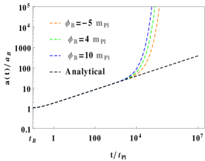
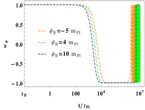
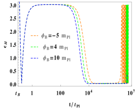
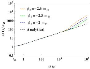
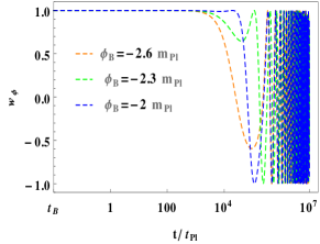
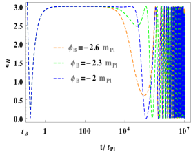
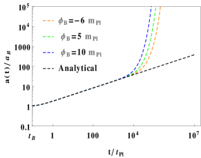
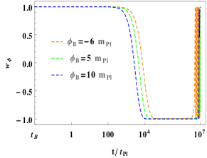
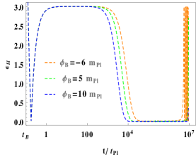
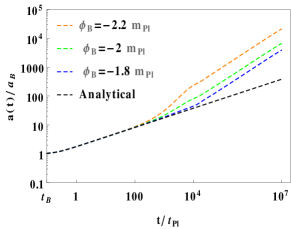
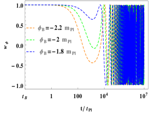
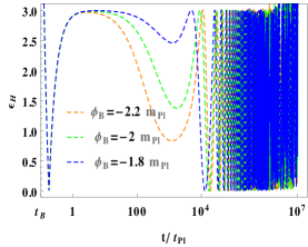
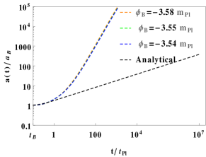
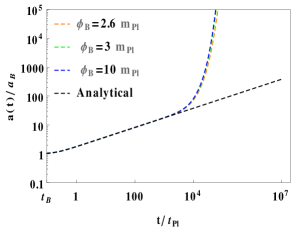
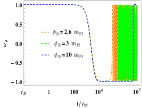
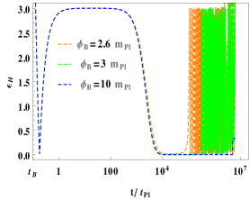
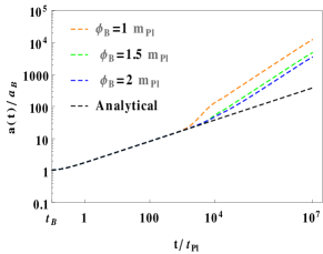
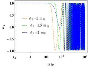
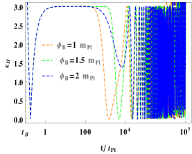
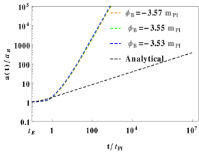
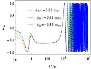
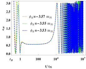
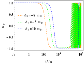
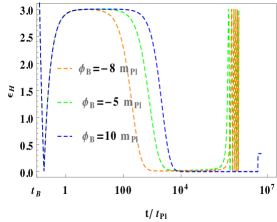
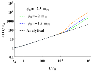
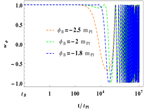
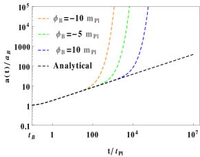
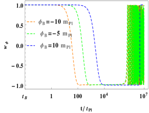
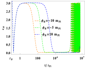
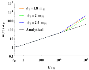
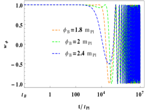
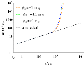
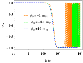
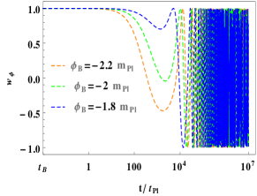
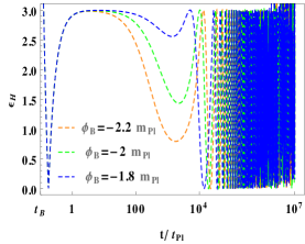
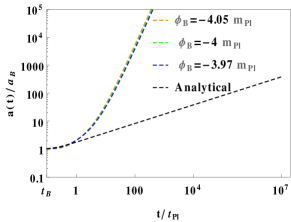
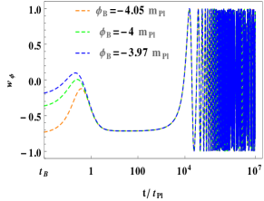
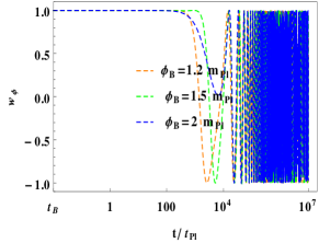
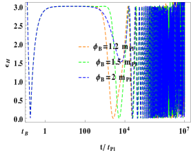
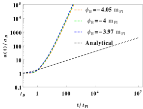
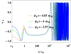
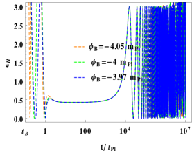
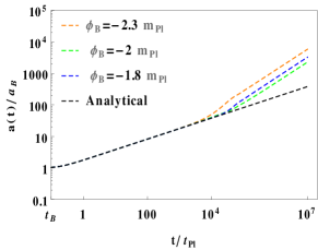
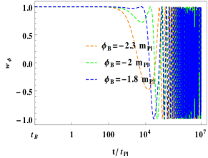
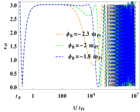
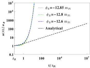
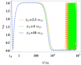
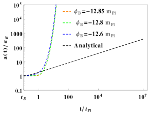
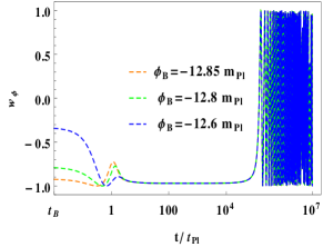
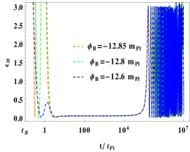
Figure 2: The numerical results for Tβˆ’m​o​d​e​lπ‘‡π‘šπ‘œπ‘‘π‘’π‘™T-model (16) with Ο•Λ™B>0subscriptΛ™italic-ϕ𝐡0\dot{\phi}_{B}>0. The figure shows the evolution of a​(t)π‘Žπ‘‘a(t), w​(Ο•)𝑀italic-Ο•w(\phi) and Ο΅Hsubscriptitalic-ϡ𝐻\epsilon_{H} for the KED with slow-roll inflation (top) and without slow-roll inflation (bottom) initial conditions at the quantum bounce. The analytical solution of a​(t)π‘Žπ‘‘a(t) [Eq.(12)] is also displayed in order to compare it with the numerical solutions. We use Ξ±=10​mP​l2𝛼10superscriptsubscriptπ‘šπ‘ƒπ‘™2\alpha=10m_{Pl}^{2}, c=1.8Γ—10βˆ’5​mP​l𝑐1.8superscript105subscriptπ‘šπ‘ƒπ‘™c=1.8\times 10^{-5}m_{Pl}, and mP​l=1subscriptπ‘šπ‘ƒπ‘™1m_{Pl}=1. Due to the symmetric nature of the Tβˆ’m​o​d​e​lπ‘‡π‘šπ‘œπ‘‘π‘’π‘™T-model, similar results can be obtained for Ο•Λ™B<0subscriptΛ™italic-ϕ𝐡0\dot{\phi}_{B}<0.
Refer to caption Refer to caption Refer to caption
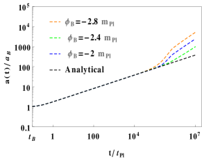
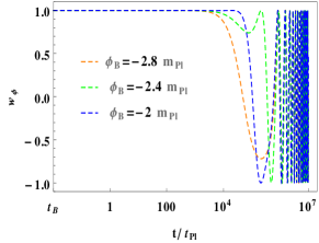
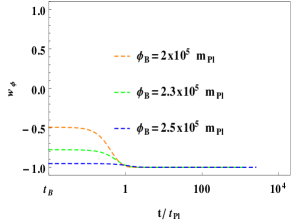
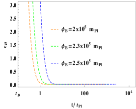
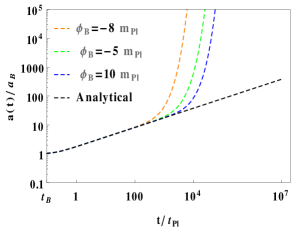
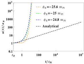
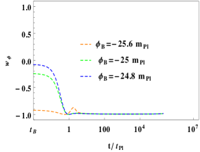
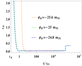
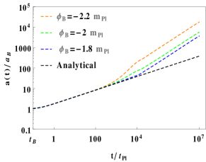
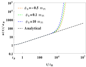
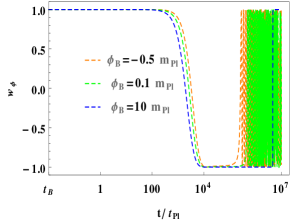
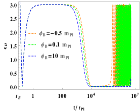
Figure 3: This figure represents the evolution of a​(t)π‘Žπ‘‘a(t), w​(Ο•)𝑀italic-Ο•w(\phi) and Ο΅Hsubscriptitalic-ϡ𝐻\epsilon_{H} for Tβˆ’m​o​d​e​lπ‘‡π‘šπ‘œπ‘‘π‘’π‘™T-model with Ο•Λ™B>0subscriptΛ™italic-ϕ𝐡0\dot{\phi}_{B}>0. Top and middle panels correspond to the KED initial conditions with and without slow-roll inflation, whereas bottom ones are for PED initial conditions having slow-roll inflation. The numerical evolution of a​(t)π‘Žπ‘‘a(t) with the analytical solution (12) is universal in the case of KED initial conditions (top and middle), while it is lost in the PED case (bottom). We take Ξ±=1010​mP​l2𝛼superscript1010superscriptsubscriptπ‘šπ‘ƒπ‘™2\alpha=10^{10}m_{Pl}^{2}, c=8.2Γ—10βˆ’6​mP​l𝑐8.2superscript106subscriptπ‘šπ‘ƒπ‘™c=8.2\times 10^{-6}m_{Pl}, and mP​l=1subscriptπ‘šπ‘ƒπ‘™1m_{Pl}=1. In the case of Ο•Λ™B<0subscriptΛ™italic-ϕ𝐡0\dot{\phi}_{B}<0, one can obtain similar results as the potential (16) is symmetric.
Refer to caption Refer to caption Refer to caption
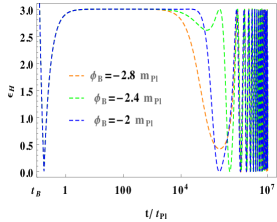
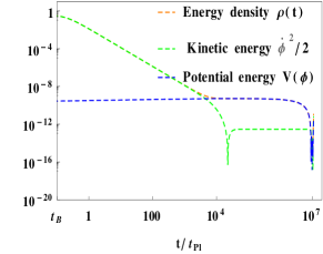
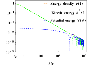
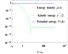
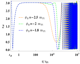
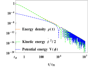
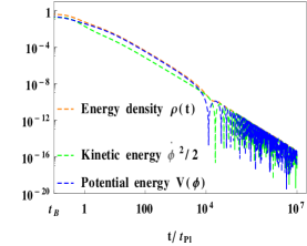
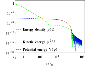
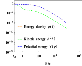
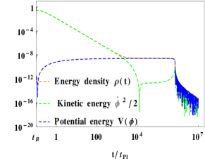
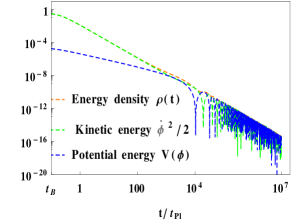
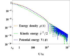
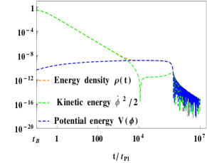
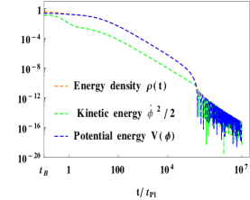
Figure 4: This figure shows the evolutions of the kinetic Ο•Λ™2/2superscriptΛ™italic-Ο•22\dot{\phi}^{2}/2 and potential V​(Ο•)𝑉italic-Ο•V(\phi) energies of the inflaton for Tβˆ’m​o​d​e​lπ‘‡π‘šπ‘œπ‘‘π‘’π‘™T-model with Ξ±=1010​mP​l2𝛼superscript1010superscriptsubscriptπ‘šπ‘ƒπ‘™2\alpha=10^{10}m_{Pl}^{2} for Ο•Λ™B>0subscriptΛ™italic-ϕ𝐡0\dot{\phi}_{B}>0. The energy density ρ=Ο•Λ™2/2+V​(Ο•)𝜌superscriptΛ™italic-Ο•22𝑉italic-Ο•\rho=\dot{\phi}^{2}/2+V(\phi) is also displayed. Left (KED case, Ο•B=5​mP​lsubscriptitalic-ϕ𝐡5subscriptπ‘šπ‘ƒπ‘™\phi_{B}=5m_{Pl}): during the bouncing phase, PE is sub-dominant and remains so until the transition phase. Thereafter, it overtakes KE and starts to dominate the evolution of the universe, whereby a slow-roll inflationary phase is resulted. Middle (KED case, Ο•B=βˆ’2.4​mP​lsubscriptitalic-ϕ𝐡2.4subscriptπ‘šπ‘ƒπ‘™\phi_{B}=-2.4m_{Pl}): This panel shows that the PE remains sub-dominant and is never able to overtake the KE. Hence, it does not give rise to a slow-roll inflationary phase. Right (PED case, Ο•B=2Γ—105​mP​lsubscriptitalic-ϕ𝐡2superscript105subscriptπ‘šπ‘ƒπ‘™\phi_{B}=2\times 10^{5}m_{Pl}): in this case, PE dominates throughout the whole evolution, and provides a slow-roll inflationary phase for a long period.
Table 1: Table for the range of α𝛼\alpha having slow-roll (SR)//no slow-roll (NSR) inflation in the cases of both KED and PED initial conditions of the inflaton field at the bounce. For the sake of simplicity, we numerically choose wΟ•β‰ƒβˆ’0.999similar-to-or-equalssubscript𝑀italic-Ο•0.999w_{\phi}\simeq-0.999 and ϡ≃10βˆ’2βˆ’10βˆ’6similar-to-or-equalsitalic-Ο΅superscript102superscript106\epsilon\simeq 10^{-2}-10^{-6} in the case of SR whereas wΟ•β‰ƒβˆ’0.94similar-to-or-equalssubscript𝑀italic-Ο•0.94w_{\phi}\simeq-0.94 and ϡ≃0.10similar-to-or-equalsitalic-Ο΅0.10\epsilon\simeq 0.10 for NSR. The solid line (βˆ’)(-) corresponds to the PED range that does not exist throughout the bouncing regime.
Model        α𝛼\alpha Slow-roll inflation depending on the range of Ο•Bsubscriptitalic-ϕ𝐡\phi_{B}
KED (SR) Existence of KED PED (SR)
(except subset) subset (NSR)
T𝑇T 0<Ξ±<4.3Γ—1090𝛼4.3superscript1090<\alpha<4.3\times 10^{9} All Yes βˆ’-
4.3Γ—109≀α4.3superscript109𝛼4.3\times 10^{9}\leq\alpha All Yes All
E𝐸E 0<Ξ±<0.020𝛼0.020<\alpha<0.02 All No (for Ο•Λ™>0Λ™italic-Ο•0\dot{\phi}>0) All
Yes (for Ο•Λ™<0Λ™italic-Ο•0\dot{\phi}<0)
0.02≀α<0.60.02𝛼0.60.02\leq\alpha<0.6 All Yes None
0.6≀α0.6𝛼0.6\leq\alpha All Yes All
n=2𝑛2n=2 0<Ξ±<0.10𝛼0.10<\alpha<0.1 All No (for Ο•Λ™>0Λ™italic-Ο•0\dot{\phi}>0) All
Yes (for Ο•Λ™<0Λ™italic-Ο•0\dot{\phi}<0)
0.1≀α<2.40.1𝛼2.40.1\leq\alpha<2.4 All Yes None
2.4≀α2.4𝛼2.4\leq\alpha All Yes All
Table 2: Table for SR//NSR with the range of Ο•Bsubscriptitalic-ϕ𝐡\phi_{B} for Ο•Λ™B>0subscriptΛ™italic-ϕ𝐡0\dot{\phi}_{B}>0 and Ο•Λ™B<0subscriptΛ™italic-ϕ𝐡0\dot{\phi}_{B}<0 having different values of α𝛼\alpha. For each value of α𝛼\alpha, the corresponding values of c𝑐c are given by Eqs.(17), (19) and (21). The sign (βˆ’)(-) represents the case in which a single initial value of Ο•Bsubscriptitalic-ϕ𝐡\phi_{B} does not provide KED=PED (wB=0)superscript𝑀𝐡0(w^{B}=0) and PED (wB<0)superscript𝑀𝐡0(w^{B}<0) at the bounce. Here, Ο•m​a​xsubscriptitalic-Ο•π‘šπ‘Žπ‘₯\phi_{max} corresponds to Tβˆ’m​o​d​e​lπ‘‡π‘šπ‘œπ‘‘π‘’π‘™T-model and given by Eq.(26). In the case of Eβˆ’m​o​d​e​lπΈπ‘šπ‘œπ‘‘π‘’π‘™E-model and Ξ±βˆ’limit-from𝛼\alpha-model with n=2𝑛2n=2, Ο•m​i​nsubscriptitalic-Ο•π‘šπ‘–π‘›\phi_{min} are given by Eqs.(29) and (37), respectively.
Model Ο•Λ™BsubscriptΛ™italic-ϕ𝐡\dot{\phi}_{B} α𝛼\alpha KED (SR) Subset of KED (NSR) KED=PED (SR/NSR) PED (SR)
(wB>0)superscript𝑀𝐡0(w^{B}>0) (wB>0)superscript𝑀𝐡0(w^{B}>0) (wB=0)superscript𝑀𝐡0(w^{B}=0) (wB<0)superscript𝑀𝐡0(w^{B}<0)
T𝑇T >0absent0>0 10 βˆ’βˆžβ‰€Ο•Bβ‰€βˆ’3.1subscriptitalic-ϕ𝐡3.1-\infty\leq\phi_{B}\leq-3.1 βˆ’3.1<Ο•Bβ‰€βˆ’1.63.1subscriptitalic-ϕ𝐡1.6-3.1<\phi_{B}\leq-1.6 βˆ’- βˆ’-
βˆ’1.61≀ϕB≀+∞1.61subscriptitalic-ϕ𝐡-1.61\leq\phi_{B}\leq+\infty
1010superscript101010^{10} βˆ’1.52Γ—105<Ο•Bβ‰€βˆ’3.211.52superscript105subscriptitalic-ϕ𝐡3.21-1.52\times 10^{5}<\phi_{B}\leq-3.21 βˆ’3.2≀ϕB<βˆ’1.83.2subscriptitalic-ϕ𝐡1.8-3.2\leq\phi_{B}<-1.8 Ο•B=Β±1.52Γ—105subscriptitalic-ϕ𝐡plus-or-minus1.52superscript105\phi_{B}=\pm 1.52\times 10^{5}(SR) βˆ’Ο•m​a​x≀ϕB<βˆ’1.52Γ—105subscriptitalic-Ο•π‘šπ‘Žπ‘₯subscriptitalic-ϕ𝐡1.52superscript105-\phi_{max}\leq\phi_{B}<-1.52\times 10^{5}
βˆ’1.8≀ϕB<1.52Γ—1051.8subscriptitalic-ϕ𝐡1.52superscript105-1.8\leq\phi_{B}<1.52\times 10^{5} 1.52Γ—105<Ο•B≀+Ο•m​a​x1.52superscript105subscriptitalic-ϕ𝐡subscriptitalic-Ο•π‘šπ‘Žπ‘₯1.52\times 10^{5}<\phi_{B}\leq+\phi_{max}
E𝐸E >0absent0>0 0.1 βˆ’1.51≀ϕBβ‰€βˆž1.51subscriptitalic-ϕ𝐡-1.51\leq\phi_{B}\leq\infty βˆ’3.52<Ο•Bβ‰€βˆ’1.53.52subscriptitalic-ϕ𝐡1.5-3.52<\phi_{B}\leq-1.5 Ο•B=βˆ’3.52subscriptitalic-ϕ𝐡3.52\phi_{B}=-3.52 (NSR) None
5 βˆ’24.70≀ϕBβ‰€βˆ’3.1124.70subscriptitalic-ϕ𝐡3.11-24.70\leq\phi_{B}\leq-3.11 βˆ’3.1≀ϕB<βˆ’1.43.1subscriptitalic-ϕ𝐡1.4-3.1\leq\phi_{B}<-1.4 Ο•B=βˆ’24.71subscriptitalic-ϕ𝐡24.71\phi_{B}=-24.71 (SR) Ο•m​i​n≀ϕBβ‰€βˆ’24.72subscriptitalic-Ο•π‘šπ‘–π‘›subscriptitalic-ϕ𝐡24.72\phi_{min}\leq\phi_{B}\leq-24.72
& βˆ’1.4≀ϕBβ‰€βˆž1.4subscriptitalic-ϕ𝐡-1.4\leq\phi_{B}\leq\infty
<0absent0<0 0.1 2.4≀ϕBβ‰€βˆž2.4subscriptitalic-ϕ𝐡2.4\leq\phi_{B}\leq\infty βˆ’3.51<Ο•B<2.43.51subscriptitalic-ϕ𝐡2.4-3.51<\phi_{B}<2.4 Ο•B=βˆ’3.51subscriptitalic-ϕ𝐡3.51\phi_{B}=-3.51 (NSR) None
5 βˆ’24.69≀ϕB≀1.424.69subscriptitalic-ϕ𝐡1.4-24.69\leq\phi_{B}\leq 1.4 1.4<Ο•B<31.4subscriptitalic-ϕ𝐡31.4<\phi_{B}<3 Ο•B=βˆ’24.7subscriptitalic-ϕ𝐡24.7\phi_{B}=-24.7 (SR) Ο•m​i​n≀ϕBβ‰€βˆ’24.71subscriptitalic-Ο•π‘šπ‘–π‘›subscriptitalic-ϕ𝐡24.71\phi_{min}\leq\phi_{B}\leq-24.71
& 3≀ϕBβ‰€βˆž3subscriptitalic-ϕ𝐡3\leq\phi_{B}\leq\infty
n=2𝑛2n=2 >0absent0>0 0.5 βˆ’1.39≀ϕBβ‰€βˆž1.39subscriptitalic-ϕ𝐡-1.39\leq\phi_{B}\leq\infty βˆ’3.93<Ο•Bβ‰€βˆ’1.43.93subscriptitalic-ϕ𝐡1.4-3.93<\phi_{B}\leq-1.4 Ο•B=βˆ’3.93subscriptitalic-ϕ𝐡3.93\phi_{B}=-3.93 (NSR) None
5 βˆ’12.4≀ϕBβ‰€βˆ’3.412.4subscriptitalic-ϕ𝐡3.4-12.4\leq\phi_{B}\leq-3.4 βˆ’3.4<Ο•B<βˆ’1.43.4subscriptitalic-ϕ𝐡1.4-3.4<\phi_{B}<-1.4 Ο•B=βˆ’12.41subscriptitalic-ϕ𝐡12.41\phi_{B}=-12.41 (SR) Ο•m​i​n≀ϕBβ‰€βˆ’12.42subscriptitalic-Ο•π‘šπ‘–π‘›subscriptitalic-ϕ𝐡12.42\phi_{min}\leq\phi_{B}\leq-12.42
& βˆ’1.4≀ϕBβ‰€βˆž1.4subscriptitalic-ϕ𝐡-1.4\leq\phi_{B}\leq\infty
<0absent0<0 0.5 2.4≀ϕBβ‰€βˆž2.4subscriptitalic-ϕ𝐡2.4\leq\phi_{B}\leq\infty βˆ’3.92<Ο•B<2.43.92subscriptitalic-ϕ𝐡2.4-3.92<\phi_{B}<2.4 Ο•B=βˆ’3.92subscriptitalic-ϕ𝐡3.92\phi_{B}=-3.92 (NSR) None
5 βˆ’12.39≀ϕB≀112.39subscriptitalic-ϕ𝐡1-12.39\leq\phi_{B}\leq 1 1<Ο•B<2.71subscriptitalic-ϕ𝐡2.71<\phi_{B}<2.7 Ο•B=βˆ’12.4subscriptitalic-ϕ𝐡12.4\phi_{B}=-12.4 (SR) Ο•m​i​n≀ϕBβ‰€βˆ’12.41subscriptitalic-Ο•π‘šπ‘–π‘›subscriptitalic-ϕ𝐡12.41\phi_{min}\leq\phi_{B}\leq-12.41
& 2.7≀ϕBβ‰€βˆž2.7subscriptitalic-ϕ𝐡2.7\leq\phi_{B}\leq\infty
Table 3: This table corresponds to the Tβˆ’m​o​d​e​lπ‘‡π‘šπ‘œπ‘‘π‘’π‘™T-model. We display the number of e𝑒e-foldings Ni​n​fsubscript𝑁𝑖𝑛𝑓N_{inf} and other parameters for different choices of Ο•Bsubscriptitalic-ϕ𝐡\phi_{B} in two cases of α𝛼\alpha, see Eq.(17). This table is for Ο•Λ™B>0subscriptΛ™italic-ϕ𝐡0\dot{\phi}_{B}>0. Due to the symmetric nature of the Tβˆ’m​o​d​e​lπ‘‡π‘šπ‘œπ‘‘π‘’π‘™T-model, one can obtain similar results for Ο•Λ™B<0subscriptΛ™italic-ϕ𝐡0\dot{\phi}_{B}<0.
α𝛼\alpha Ο•Bsubscriptitalic-ϕ𝐡\phi_{B} Inflation t/tp​l𝑑subscript𝑑𝑝𝑙t/t_{pl} Ο΅italic-Ο΅\epsilon w𝑀w Ni​n​fsubscript𝑁𝑖𝑛𝑓N_{inf} Β Β Β rwc/rwsuperscriptsubscriptπ‘Ÿπ‘€π‘subscriptπ‘Ÿπ‘€r_{w}^{c}/r_{w} Β Β Β wBsuperscript𝑀𝐡{w}^{B}
10 βˆ’5.35.3-5.3 begin 5.40007Γ—1035.40007superscript1035.40007\times 10^{3} 0.99 βˆ’1/313-1/3
slow-roll 4.66194Γ—1044.66194superscript1044.66194\times 10^{4} 5.0Γ—10βˆ’35.0superscript1035.0\times 10^{-3} βˆ’0.9960.996-0.996 79.23 rwc<rwsuperscriptsubscriptπ‘Ÿπ‘€π‘subscriptπ‘Ÿπ‘€r_{w}^{c}<r_{w} >0absent0>0
end 2.032Γ—1062.032superscript1062.032\times 10^{6} 1.0 βˆ’1/313-1/3
βˆ’4.94.9-4.9 begin 6.05487Γ—1036.05487superscript1036.05487\times 10^{3} 0.99 βˆ’1/313-1/3
slow-roll 5.01307Γ—1045.01307superscript1045.01307\times 10^{4} 7.1Γ—10βˆ’37.1superscript1037.1\times 10^{-3} βˆ’0.9940.994-0.994 60.28 rwc=rwsuperscriptsubscriptπ‘Ÿπ‘€π‘subscriptπ‘Ÿπ‘€r_{w}^{c}=r_{w} >0absent0>0
end 1.745Γ—1061.745superscript1061.745\times 10^{6} 0.99 βˆ’1/313-1/3
βˆ’44-4 begin 8.594Γ—1038.594superscript1038.594\times 10^{3} 1.0 βˆ’1/313-1/3
slow-roll 6.21983Γ—1046.21983superscript1046.21983\times 10^{4} 1.9Γ—10βˆ’21.9superscript1021.9\times 10^{-2} βˆ’0.9870.987-0.987 27.57 rwc>rwsuperscriptsubscriptπ‘Ÿπ‘€π‘subscriptπ‘Ÿπ‘€r_{w}^{c}>r_{w} >0absent0>0
end 1.133Γ—1061.133superscript1061.133\times 10^{6} 1.0 βˆ’1/313-1/3
1.11.11.1 begin 6.25705Γ—1036.25705superscript1036.25705\times 10^{3} 1.0 βˆ’1/313-1/3
slow-roll 2.04834Γ—1042.04834superscript1042.04834\times 10^{4} 3.1Γ—10βˆ’53.1superscript1053.1\times 10^{-5} βˆ’11-1 60.59 rwc=rwsuperscriptsubscriptπ‘Ÿπ‘€π‘subscriptπ‘Ÿπ‘€r_{w}^{c}=r_{w} >0absent0>0
end 1.751Γ—1061.751superscript1061.751\times 10^{6} 0.99 βˆ’1/313-1/3
222 begin 4.98597Γ—1034.98597superscript1034.98597\times 10^{3} 1.0 βˆ’1/313-1/3
slow-roll 1.7624Γ—1041.7624superscript1041.7624\times 10^{4} 1.5Γ—10βˆ’41.5superscript1041.5\times 10^{-4} βˆ’11-1 103.17 rwc<rwsuperscriptsubscriptπ‘Ÿπ‘€π‘subscriptπ‘Ÿπ‘€r_{w}^{c}<r_{w} >0absent0>0
end 2.356Γ—1062.356superscript1062.356\times 10^{6} 1.0 βˆ’1/313-1/3
1010superscript101010^{10} βˆ’5.55.5-5.5 begin 1.106433Γ—1041.106433superscript1041.106433\times 10^{4} 0.99 βˆ’1/313-1/3
slow-roll 9.60811Γ—1049.60811superscript1049.60811\times 10^{4} 7.1Γ—10βˆ’37.1superscript1037.1\times 10^{-3} βˆ’0.9950.995-0.995 77.91 rwc<rwsuperscriptsubscriptπ‘Ÿπ‘€π‘subscriptπ‘Ÿπ‘€r_{w}^{c}<r_{w} >0absent0>0
end 4.345Γ—1064.345superscript1064.345\times 10^{6} 0.99 βˆ’1/313-1/3
βˆ’5.15.1-5.1 begin 1.2549Γ—1041.2549superscript1041.2549\times 10^{4} 0.99 βˆ’1/313-1/3
slow-roll 1.04701Γ—1051.04701superscript1051.04701\times 10^{5} 8.3Γ—10βˆ’38.3superscript1038.3\times 10^{-3} βˆ’0.9940.994-0.994 60.49 rwc=rwsuperscriptsubscriptπ‘Ÿπ‘€π‘subscriptπ‘Ÿπ‘€r_{w}^{c}=r_{w} >0absent0>0
end 3.804Γ—1063.804superscript1063.804\times 10^{6} 0.99 βˆ’1/313-1/3
0.50.50.5 begin 1.57596Γ—1041.57596superscript1041.57596\times 10^{4} 0.99 βˆ’1/313-1/3
slow-roll 4.82807Γ—1044.82807superscript1044.82807\times 10^{4} 1.2Γ—10βˆ’41.2superscript1041.2\times 10^{-4} βˆ’11-1 41.88 rwc>rwsuperscriptsubscriptπ‘Ÿπ‘€π‘subscriptπ‘Ÿπ‘€r_{w}^{c}>r_{w} >0absent0>0
end 3.13Γ—1063.13superscript1063.13\times 10^{6} 0.99 βˆ’1/313-1/3
1.051.051.05 begin 1.30481Γ—1041.30481superscript1041.30481\times 10^{4} 0.99 βˆ’1/313-1/3
slow-roll 4.19299Γ—1044.19299superscript1044.19299\times 10^{4} 1.3Γ—10βˆ’51.3superscript1051.3\times 10^{-5} βˆ’11-1 60.32 rwc=rwsuperscriptsubscriptπ‘Ÿπ‘€π‘subscriptπ‘Ÿπ‘€r_{w}^{c}=r_{w} >0absent0>0
end 3.8Γ—1063.8superscript1063.8\times 10^{6} 0.99 βˆ’1/313-1/3
1.51.51.5 begin 1.14255Γ—1041.14255superscript1041.14255\times 10^{4} 0.99 βˆ’1/313-1/3
slow-roll 3.79398Γ—1043.79398superscript1043.79398\times 10^{4} 3.4Γ—10βˆ’53.4superscript1053.4\times 10^{-5} βˆ’11-1 78.09 rwc<rwsuperscriptsubscriptπ‘Ÿπ‘€π‘subscriptπ‘Ÿπ‘€r_{w}^{c}<r_{w} >0absent0>0
end 4.354Γ—1064.354superscript1064.354\times 10^{6} 1.00 βˆ’1/313-1/3
2Γ—1052superscript1052\times 10^{5} begin 0.010.010.01 1.0 βˆ’0.4920.492-0.492
slow-roll 1.01.01.0 0.0470.0470.047 βˆ’0.9840.984-0.984 713.98 rwc<rwsuperscriptsubscriptπ‘Ÿπ‘€π‘subscriptπ‘Ÿπ‘€r_{w}^{c}<r_{w} <0absent0<0
end 888888888 0.1 βˆ’1/313-1/3

II Background evolution

In the framework of LQC, the modified Friedmann equation in a spatially flat Friedmann-Lemaitre-Robertson-Walker (FLRW) background is written as ashtekar2006

H2=8​π3​mP​l2​ρ​(1βˆ’ΟΟc),superscript𝐻28πœ‹3superscriptsubscriptπ‘šπ‘ƒπ‘™2𝜌1𝜌subscriptπœŒπ‘\displaystyle H^{2}=\frac{8\pi}{3m_{Pl}^{2}}~{}\rho\Big{(}1-\frac{\rho}{\rho_{c}}\Big{)}, (1)

where H=aΛ™/aπ»Λ™π‘Žπ‘ŽH=\dot{a}/a is the Hubble parameter, ρ=Ο•Λ™2/2+V​(Ο•)𝜌superscriptΛ™italic-Ο•22𝑉italic-Ο•\rho=\dot{\phi}^{2}/2+V(\phi) represents the energy density of the inflaton field, and V​(Ο•)𝑉italic-Ο•V(\phi) is the potential of the field. The dot denotes a derivative with respect to the cosmic time t𝑑t, mP​lsubscriptπ‘šπ‘ƒπ‘™m_{Pl} is the Planck mass and ρcsubscriptπœŒπ‘\rho_{c} is the critical energy density that corresponds to the maximum value of energy density, and is given by ρc≃0.41​mp​l4similar-to-or-equalssubscriptπœŒπ‘0.41superscriptsubscriptπ‘šπ‘π‘™4\rho_{c}\simeq 0.41m_{pl}^{4} Meissne ; Domagala .

The conservation equation in the context of LQC remains the same as in the classical theory

ρ˙+3​H​(ρ+p)=0.Λ™πœŒ3π»πœŒπ‘0\displaystyle\dot{\rho}+3H(\rho+p)=0. (2)

Here, p𝑝p denotes the pressure of the matter field. Eq.(2) gives the Klein-Gordon equation for a single scalar field

ϕ¨+3​H​ϕ˙+d​V​(Ο•)d​ϕ=0.Β¨italic-Ο•3𝐻˙italic-ϕ𝑑𝑉italic-ϕ𝑑italic-Ο•0\displaystyle\ddot{\phi}+3H\dot{\phi}+\frac{dV(\phi)}{d\phi}=0. (3)

Eq.(1) tells that at ρ=ρc𝜌subscriptπœŒπ‘\rho=\rho_{c}, H=0𝐻0H=0 that means quantum bounce occurs at ρ=ρc𝜌subscriptπœŒπ‘\rho=\rho_{c}. The numerical evolution of the background with the bouncing phase has been extensively studied in the literature. One of the main results is that a desired slow-roll inflation is achieved psingh2006 ; Mielczarek ; zhang2007 ; chen2015 ; alam2017 ; Tao2017a ; Tao2017b ; ashtekar2011 . Keeping this in mind, we shall study β€œbounce and slow-roll” with the generalized Ξ±βˆ’limit-from𝛼\alpha-attractor model (see Sec. III).

Let us first examine the evolution equations for a general potential V​(Ο•)𝑉italic-Ο•V(\phi). We numerically solve Eqs.(1) and (3) with the initial values of a​(t)π‘Žπ‘‘a(t), ϕ​(t)italic-ϕ𝑑\phi(t) and ϕ˙​(t)Λ™italic-ϕ𝑑\dot{\phi}(t) at a specific time. A natural option of the time is at the bounce t=tB𝑑subscript𝑑𝐡t=t_{B}, for which we have

ρ𝜌\displaystyle\rho =\displaystyle= ρc=12​ϕ˙2​(tB)+V​(ϕ​(tB)),subscriptπœŒπ‘12superscriptΛ™italic-Ο•2subscript𝑑𝐡𝑉italic-Ο•subscript𝑑𝐡\displaystyle\rho_{c}=\frac{1}{2}\dot{\phi}^{2}(t_{B})+V(\phi(t_{B})),
a˙​(tB)Λ™π‘Žsubscript𝑑𝐡\displaystyle\dot{a}(t_{B}) =\displaystyle= 0,0\displaystyle 0, (4)

from which we find

ϕ˙​(tB)Λ™italic-Ο•subscript𝑑𝐡\displaystyle\dot{\phi}(t_{B}) =\displaystyle= Β±2​(ρcβˆ’V​(ϕ​(tB))).plus-or-minus2subscriptπœŒπ‘π‘‰italic-Ο•subscript𝑑𝐡\displaystyle\pm\sqrt{2\Big{(}\rho_{c}-V(\phi(t_{B}))\Big{)}}. (5)

Without loss of the generality, we can always choose

a​(tB)π‘Žsubscript𝑑𝐡\displaystyle a(t_{B}) =\displaystyle= 1.1\displaystyle 1. (6)

Hereafter, we shall read ϕ​(tB)italic-Ο•subscript𝑑𝐡\phi(t_{B}) and ϕ˙​(tB)Λ™italic-Ο•subscript𝑑𝐡\dot{\phi}(t_{B}) as Ο•Bsubscriptitalic-ϕ𝐡\phi_{B} and Ο•Λ™BsubscriptΛ™italic-ϕ𝐡\dot{\phi}_{B}. From Eq.(5), one can clearly see that for a given potential, the initial values will be uniquely identified by Ο•Bsubscriptitalic-ϕ𝐡\phi_{B} only. Subsequently, we shall consider two cases: (a) PIV:Β Β  Ο•Λ™B>0subscriptΛ™italic-ϕ𝐡0\dot{\phi}_{B}>0 and (b) NIV: Β Ο•Λ™B<0subscriptΛ™italic-ϕ𝐡0\dot{\phi}_{B}<0.

Second, we introduce the following quantities that are essential for this paper alam2017 ; Tao2017a ; Tao2017b .

(1) The equation of state (EoS) w​(Ο•)𝑀italic-Ο•w(\phi) for the inflaton field is defined as

w​(Ο•)=Ο•Λ™2/2βˆ’V​(Ο•)Ο•Λ™2/2+V​(Ο•).𝑀italic-Ο•superscriptΛ™italic-Ο•22𝑉italic-Ο•superscriptΛ™italic-Ο•22𝑉italic-Ο•\displaystyle w(\phi)=\frac{\dot{\phi}^{2}/2-V(\phi)}{\dot{\phi}^{2}/2+V(\phi)}. (7)

In the slow-roll inflationary phase, w​(Ο•)β‰ƒβˆ’1similar-to-or-equals𝑀italic-Ο•1w(\phi)\simeq-1.

To differentiate the initial conditions for being dominated by the kinetic energy (KE) or potential energy (PE) at the bounce, we also introduce the quantity wBsuperscript𝑀𝐡w^{B}, so that

wB≑w​(Ο•)|Ο•=Ο•B={>0,KE>PE=0,KE=PE<0,KE<PEsuperscript𝑀𝐡evaluated-at𝑀italic-Ο•italic-Ο•subscriptitalic-ϕ𝐡casesformulae-sequenceabsent0KEPEotherwiseformulae-sequenceabsent0KEPEotherwiseformulae-sequenceabsent0KEPEotherwisew^{B}\equiv w(\phi)\Big{|}_{\phi=\phi_{B}}=\begin{cases}>0,\qquad\text{KE}>\text{PE}\\ =0,\qquad\text{KE}=\text{PE}\\ <0,\qquad\text{KE}<\text{PE}\end{cases} (8)

(2) The slow-roll parameter ϡHsubscriptitalic-ϡ𝐻\epsilon_{H}, that is expressed in terms of the Hubble parameter and its derivatives,

Ο΅H=βˆ’HΛ™H2.subscriptitalic-ϡ𝐻˙𝐻superscript𝐻2\displaystyle\epsilon_{H}=-\frac{\dot{H}}{H^{2}}. (9)

During the slow-roll inflation, Ο΅Hβ‰ͺ1much-less-thansubscriptitalic-ϡ𝐻1\epsilon_{H}\ll 1.

(3) The number of e𝑒e-folds Ni​n​fsubscript𝑁𝑖𝑛𝑓N_{inf} during the slow-roll inflation is given by

Ni​n​f=l​n​(ae​n​dai)=∫tite​n​dH​(t)​𝑑tsubscript𝑁𝑖𝑛𝑓𝑙𝑛subscriptπ‘Žπ‘’π‘›π‘‘subscriptπ‘Žπ‘–superscriptsubscriptsubscript𝑑𝑖subscript𝑑𝑒𝑛𝑑𝐻𝑑differential-d𝑑\displaystyle N_{inf}=ln\Big{(}\frac{a_{end}}{a_{i}}\Big{)}=\int_{t_{i}}^{t_{end}}H(t)dt
=βˆ«Ο•iΟ•e​n​dHΟ•Λ™β€‹π‘‘Ο•β‰ƒβˆ«Ο•e​n​dΟ•iVVϕ​𝑑ϕ,absentsuperscriptsubscriptsubscriptitalic-ϕ𝑖subscriptitalic-ϕ𝑒𝑛𝑑𝐻˙italic-Ο•differential-ditalic-Ο•similar-to-or-equalssuperscriptsubscriptsubscriptitalic-ϕ𝑒𝑛𝑑subscriptitalic-ϕ𝑖𝑉subscript𝑉italic-Ο•differential-ditalic-Ο•\displaystyle=\int_{\phi_{i}}^{\phi_{end}}\frac{H}{\dot{\phi}}d\phi\simeq\int_{\phi_{end}}^{\phi_{i}}\frac{V}{V_{\phi}}d\phi, (10)

where aisubscriptπ‘Žπ‘–a_{i} (ae​n​dsubscriptπ‘Žπ‘’π‘›π‘‘a_{end}) represents the expansion factor when the inflation starts (ends), i.e. a¨​(ti)≳0greater-than-or-equivalent-toΒ¨π‘Žsubscript𝑑𝑖0\ddot{a}(t_{i})\gtrsim 0 and w​(Ο•e​n​d)=βˆ’1/3𝑀subscriptitalic-ϕ𝑒𝑛𝑑13w(\phi_{end})=-1/3.

(4) Using Eqs.(1) and (3), we obtain an analytical expression of the scale factor a​(t)π‘Žπ‘‘a(t) during the bouncing phase. In this phase, if the potential is very small compared to the kinetic energy, then Eqs.(1) and (3) become

H2=8​π3​mP​l2​12​ϕ2˙​(1βˆ’Ο•2Λ™2​ρc),superscript𝐻28πœ‹3superscriptsubscriptπ‘šπ‘ƒπ‘™212Λ™superscriptitalic-Ο•21Λ™superscriptitalic-Ο•22subscriptπœŒπ‘\displaystyle H^{2}=\frac{8\pi}{3m_{Pl}^{2}}~{}\frac{1}{2}\dot{\phi^{2}}\Big{(}1-\frac{\dot{\phi^{2}}}{2\rho_{c}}\Big{)},
ϕ¨+3​H​ϕ˙=0.Β¨italic-Ο•3𝐻˙italic-Ο•0\displaystyle\ddot{\phi}+3H\dot{\phi}=0. (11)

We solve the above equations analytically, and find alam2017 ; Tao2017a ; Tao2017b

Ο•Λ™Λ™italic-Ο•\displaystyle\dot{\phi} =\displaystyle= Β±2​ρc​(aBa​(t))3,plus-or-minus2subscriptπœŒπ‘superscriptsubscriptπ‘Žπ΅π‘Žπ‘‘3\displaystyle\pm\sqrt{2\rho_{c}}\left(\frac{a_{B}}{a(t)}\right)^{3},
a​(t)π‘Žπ‘‘\displaystyle a(t) =\displaystyle= aB​(1+δ​t2tP​l2)1/6,subscriptπ‘Žπ΅superscript1𝛿superscript𝑑2superscriptsubscript𝑑𝑃𝑙216\displaystyle a_{B}\left(1+\delta\frac{t^{2}}{t_{Pl}^{2}}\right)^{1/6}, (12)

where tP​lsubscript𝑑𝑃𝑙t_{Pl} denotes the Planck time, and Ξ΄=24​π​ρc/mP​l4𝛿24πœ‹subscriptπœŒπ‘superscriptsubscriptπ‘šπ‘ƒπ‘™4\delta={24\pi\rho_{c}}/{m_{Pl}^{4}} is a dimensionless parameter.

(5) We define a quantity rwsubscriptπ‘Ÿπ‘€r_{w}, that is the ratio between the kinetic and potential energies,

rwsubscriptπ‘Ÿπ‘€\displaystyle r_{w} ≑\displaystyle\equiv 12​ϕ˙2V​(Ο•).12superscriptΛ™italic-Ο•2𝑉italic-Ο•\displaystyle\frac{\frac{1}{2}\dot{\phi}^{2}}{V(\phi)}. (13)

Following Eq.(13), one can define rwcsuperscriptsubscriptπ‘Ÿπ‘€π‘r_{w}^{c} that corresponds to Ni​n​f≃60similar-to-or-equalssubscript𝑁𝑖𝑛𝑓60N_{inf}\simeq 60 during the slow-roll inflation,

rwc≑12​ϕ˙2V​(Ο•)|Ni​n​f≃60={rwc>rwNi​n​f<60rwc=rwNi​n​f≃60rwc<rwNi​n​f>60.superscriptsubscriptπ‘Ÿπ‘€π‘evaluated-at12superscriptΛ™italic-Ο•2𝑉italic-Ο•similar-to-or-equalssubscript𝑁𝑖𝑛𝑓60casesformulae-sequencesuperscriptsubscriptπ‘Ÿπ‘€π‘subscriptπ‘Ÿπ‘€subscript𝑁𝑖𝑛𝑓60otherwiseformulae-sequencesuperscriptsubscriptπ‘Ÿπ‘€π‘subscriptπ‘Ÿπ‘€similar-to-or-equalssubscript𝑁𝑖𝑛𝑓60otherwiseformulae-sequencesuperscriptsubscriptπ‘Ÿπ‘€π‘subscriptπ‘Ÿπ‘€subscript𝑁𝑖𝑛𝑓60otherwiser_{w}^{c}\equiv\frac{\frac{1}{2}\dot{\phi}^{2}}{V(\phi)}\Big{|}_{N_{inf}\simeq 60}=\begin{cases}r_{w}^{c}>r_{w}\qquad N_{inf}<60\\ r_{w}^{c}=r_{w}\qquad N_{inf}\simeq 60\\ r_{w}^{c}<r_{w}\qquad N_{inf}>60.\end{cases} (14)

In the following section, we shall discuss the generalized Ξ±βˆ’limit-from𝛼\alpha-attractor model in the context of PIV and NIV at the quantum bounce.

III Ξ±βˆ’limit-from𝛼\alpha-attractor model

In this section, we shall study β€œbounce and slow-roll” with the generalized Ξ±βˆ’limit-from𝛼\alpha-attractor model in the framework of LQC. Let us consider the following form of the potential alam2018 ; linder15 :

V​(Ο•)𝑉italic-Ο•\displaystyle V(\phi) =\displaystyle= α​c2​[tanh⁑(Ο•6​α)]2[1+tanh⁑(Ο•6​α)]2​n,𝛼superscript𝑐2superscriptdelimited-[]italic-Ο•6𝛼2superscriptdelimited-[]1italic-Ο•6𝛼2𝑛\displaystyle\alpha c^{2}\frac{\left[\tanh\left(\frac{\phi}{\sqrt{6\alpha}}\right)\right]^{2}}{\left[1+\tanh\left(\frac{\phi}{\sqrt{6\alpha}}\right)\right]^{2n}}, (15)

where the parameters α𝛼\alpha and c𝑐c have the dimensions of MP​l2superscriptsubscript𝑀𝑃𝑙2M_{Pl}^{2} and MP​lsubscript𝑀𝑃𝑙M_{Pl}, and MP​l=mP​l/8​πsubscript𝑀𝑃𝑙subscriptπ‘šπ‘ƒπ‘™8πœ‹M_{Pl}=m_{Pl}/\sqrt{8\pi} is the reduced Planck mass. The parameter n𝑛n takes the values n=0,1,2,3​…𝑛0123…n=0,1,2,3... For large field values (Ο•β†’βˆžβ†’italic-Ο•\phi\rightarrow\infty), the generalized Ξ±βˆ’limit-from𝛼\alpha-attractor potential becomes flatten, and for small field values (Ο•β†’0β†’italic-Ο•0\phi\rightarrow 0), it behaves as a quadratic one. For different values of n𝑛n, Eq.(15) gives the following forms of the potentials.

For n=0𝑛0n=0, we have

V​(Ο•)𝑉italic-Ο•\displaystyle V(\phi) =\displaystyle= α​c2​[tanh⁑(Ο•6​α)]2.𝛼superscript𝑐2superscriptdelimited-[]italic-Ο•6𝛼2\displaystyle\alpha c^{2}\left[\tanh\left(\frac{\phi}{\sqrt{6\alpha}}\right)\right]^{2}. (16)

In the literature, Eq.(16) is known as Tβˆ’m​o​d​e​lπ‘‡π‘šπ‘œπ‘‘π‘’π‘™T-model alpha ; alpha2 ; alpha3 , and also represents GL model for Ξ±=1/9𝛼19\alpha=1/9 GL . We find values of α𝛼\alpha and c𝑐c that are consistent with the Planck 2015 results for inflationary universe Planck2015 . Here, we write only those values which shall be used in figures and tables. However, one can also obtain other combinations (see Appendix A)

α𝛼\displaystyle\alpha =\displaystyle= 10​mP​l2,c=1.8Γ—10βˆ’5​mP​l10superscriptsubscriptπ‘šπ‘ƒπ‘™2𝑐1.8superscript105subscriptπ‘šπ‘ƒπ‘™\displaystyle 10m_{Pl}^{2},\qquad~{}~{}~{}c=1.8\times 10^{-5}m_{Pl}
α𝛼\displaystyle\alpha =\displaystyle= 1010​mP​l2,c=8.2Γ—10βˆ’6​mP​l.superscript1010superscriptsubscriptπ‘šπ‘ƒπ‘™2𝑐8.2superscript106subscriptπ‘šπ‘ƒπ‘™\displaystyle 10^{10}m_{Pl}^{2},\qquad c=8.2\times 10^{-6}m_{Pl}. (17)

For n=1𝑛1n=1, we have

V​(Ο•)𝑉italic-Ο•\displaystyle V(\phi) =\displaystyle= α​c24​(1βˆ’eβˆ’23​α​ϕ)2.𝛼superscript𝑐24superscript1superscript𝑒23𝛼italic-Ο•2\displaystyle\frac{\alpha c^{2}}{4}\left(1-e^{-\sqrt{\frac{2}{3\alpha}}\phi}\right)^{2}. (18)

This is called Eβˆ’m​o​d​e​lπΈπ‘šπ‘œπ‘‘π‘’π‘™E-model (generalization of the Starobinsky model) alpha1 . Eq.(18) corresponds to the Starobinsky model when Ξ±=1𝛼1\alpha=1 staro1980 . For the numerical evolution, combinations of α𝛼\alpha and c𝑐c that are in agreement with the Planck data Planck2015 , are given as (see Appendix A)

α𝛼\displaystyle\alpha =\displaystyle= 0.1​mP​l2,c=3.3Γ—10βˆ’4​mP​l,0.1superscriptsubscriptπ‘šπ‘ƒπ‘™2𝑐3.3superscript104subscriptπ‘šπ‘ƒπ‘™\displaystyle 0.1m_{Pl}^{2},\qquad c=3.3\times 10^{-4}m_{Pl},
α𝛼\displaystyle\alpha =\displaystyle= 5​mP​l2,c=4.9Γ—10βˆ’5​mP​l.5superscriptsubscriptπ‘šπ‘ƒπ‘™2𝑐4.9superscript105subscriptπ‘šπ‘ƒπ‘™\displaystyle 5m_{Pl}^{2},\qquad~{}~{}c=4.9\times 10^{-5}m_{Pl}. (19)

For n=2𝑛2n=2, we have

V​(Ο•)𝑉italic-Ο•\displaystyle V(\phi) =\displaystyle= α​c2​[tanh⁑(Ο•6​α)]2[1+tanh⁑(Ο•6​α)]4.𝛼superscript𝑐2superscriptdelimited-[]italic-Ο•6𝛼2superscriptdelimited-[]1italic-Ο•6𝛼4\displaystyle\alpha c^{2}\frac{\left[\tanh\left(\frac{\phi}{\sqrt{6\alpha}}\right)\right]^{2}}{\left[1+\tanh\left(\frac{\phi}{\sqrt{6\alpha}}\right)\right]^{4}}. (20)

Values of α𝛼\alpha and c𝑐c that are compatible with the Planck data Planck2015 are given by (see Appendix A)

α𝛼\displaystyle\alpha =\displaystyle= 0.5​mP​l2,c=2.9Γ—10βˆ’4​mP​l,0.5superscriptsubscriptπ‘šπ‘ƒπ‘™2𝑐2.9superscript104subscriptπ‘šπ‘ƒπ‘™\displaystyle 0.5m_{Pl}^{2},\qquad c=2.9\times 10^{-4}m_{Pl},
α𝛼\displaystyle\alpha =\displaystyle= 5​mP​l2,c=9.4Γ—10βˆ’5​mP​l.5superscriptsubscriptπ‘šπ‘ƒπ‘™2𝑐9.4superscript105subscriptπ‘šπ‘ƒπ‘™\displaystyle 5m_{Pl}^{2},\qquad~{}~{}c=9.4\times 10^{-5}m_{Pl}. (21)

Here, we are interested in the dynamics of the inflaton field having potentials (16), (18) and (20). Numerically, we shall solve Eqs.(1), (3) with (16), (18) and (20), and examine whether following the quantum bounce, a desired slow-roll inflation exists or not.

Before proceeding, let us first consider the inflationary potentials (16), (18) and (20) that are shown in Fig. 1. The predictions of Eq.(16) with (18) and (20) are similar but not identical as the main difference is in the shape of the potentials. The potential (16) is symmetric about Ο•=0italic-Ο•0\phi=0, whereas potentials (18) and (20) are not symmetric in nature.

Second, we present the range of α𝛼\alpha (depending on Ο•Bsubscriptitalic-ϕ𝐡\phi_{B}) having inflationary/non-inflationary phase for the models under consideration in Table 1. Following this, we choose some values of α𝛼\alpha in each case and use them to draw the figures with different values of Ο•Bsubscriptitalic-ϕ𝐡\phi_{B}, and its corresponding range for inflationary/non-inflationary phase with PIV and NIV are shown in Table 2.
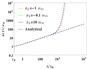
Refer to caption Refer to caption Refer to caption
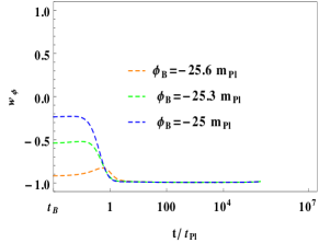
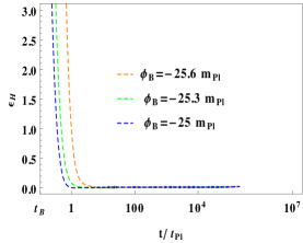
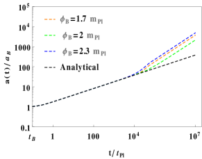
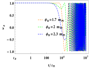
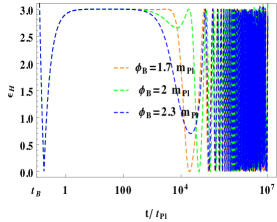
Figure 5: This figure exhibits the numerical evolution of a​(t)π‘Žπ‘‘a(t), w​(Ο•)𝑀italic-Ο•w(\phi) and Ο΅Hsubscriptitalic-ϡ𝐻\epsilon_{H} for Eβˆ’m​o​d​e​lπΈπ‘šπ‘œπ‘‘π‘’π‘™E-model (18) with Ο•Λ™B>0subscriptΛ™italic-ϕ𝐡0\dot{\phi}_{B}>0. Top and middle panels are plotted for KED initial conditions whereas bottom ones are for PED initial values. Here, only KED (except a small subset) initial values lead to the slow-roll inflationary phase, while the PED and a subset of KED initial conditions do not provide a slow-roll inflation phase. We choose Ξ±=0.1​mP​l2𝛼0.1superscriptsubscriptπ‘šπ‘ƒπ‘™2\alpha=0.1m_{Pl}^{2}, c=3.3Γ—10βˆ’4​mP​l𝑐3.3superscript104subscriptπ‘šπ‘ƒπ‘™c=3.3\times 10^{-4}m_{Pl}, and mP​l=1subscriptπ‘šπ‘ƒπ‘™1m_{Pl}=1.
Refer to caption Refer to caption Refer to caption
Figure 6: This figure is similar to Fig. 5 but with Ο•Λ™B<0subscriptΛ™italic-ϕ𝐡0\dot{\phi}_{B}<0.
Refer to caption Refer to caption Refer to caption
Figure 7: This figure is for Eβˆ’m​o​d​e​lπΈπ‘šπ‘œπ‘‘π‘’π‘™E-model (18) with Ο•Λ™B>0subscriptΛ™italic-ϕ𝐡0\dot{\phi}_{B}>0. Top (KED, except a small subset) and bottom (PED) panels represent the slow-roll inflation region whereas the middle panels (subset of KED) do not. Here, we take Ξ±=5​mP​l2𝛼5superscriptsubscriptπ‘šπ‘ƒπ‘™2\alpha=5m_{Pl}^{2}, c=4.9Γ—10βˆ’5​mP​l𝑐4.9superscript105subscriptπ‘šπ‘ƒπ‘™c=4.9\times 10^{-5}m_{Pl}, and mP​l=1subscriptπ‘šπ‘ƒπ‘™1m_{Pl}=1.
Refer to caption Refer to caption Refer to caption
Figure 8: This figure is same as Fig. 7 but with Ο•Λ™B<0subscriptΛ™italic-ϕ𝐡0\dot{\phi}_{B}<0.
Refer to caption Refer to caption Refer to caption
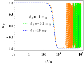
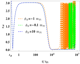
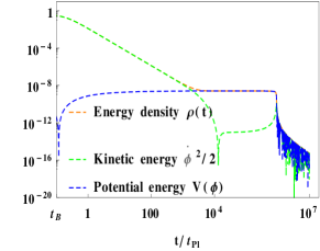
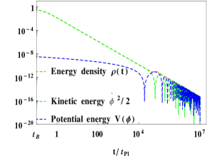
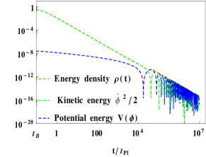
Figure 9: In this figure the kinetic and potential energies are plotted for Eβˆ’m​o​d​e​lπΈπ‘šπ‘œπ‘‘π‘’π‘™E-model with Ξ±=0.1​mP​l2𝛼0.1superscriptsubscriptπ‘šπ‘ƒπ‘™2\alpha=0.1m_{Pl}^{2} (Top) and Ξ±=5​mP​l2𝛼5superscriptsubscriptπ‘šπ‘ƒπ‘™2\alpha=5m_{Pl}^{2} (Bottom) for Ο•Λ™B>0subscriptΛ™italic-ϕ𝐡0\dot{\phi}_{B}>0. Top: left and middle panels correspond to KED initial conditions at the bounce. Left panel ( Ο•B=βˆ’0.1​mP​lsubscriptitalic-ϕ𝐡0.1subscriptπ‘šπ‘ƒπ‘™\phi_{B}=-0.1m_{Pl}) provides the slow-roll inflation as PE dominates at the later regime, while it is not possible in the middle panel ( Ο•B=βˆ’2​mP​lsubscriptitalic-ϕ𝐡2subscriptπ‘šπ‘ƒπ‘™\phi_{B}=-2m_{Pl}) as PE never dominates. Right panel ( Ο•B=βˆ’3.58​mP​lsubscriptitalic-ϕ𝐡3.58subscriptπ‘šπ‘ƒπ‘™\phi_{B}=-3.58m_{Pl}) represents the PED case, but does not yield the slow-roll inflation. Bottom: Left panel ( Ο•B=βˆ’8​mP​lsubscriptitalic-ϕ𝐡8subscriptπ‘šπ‘ƒπ‘™\phi_{B}=-8m_{Pl}) gives rise to the slow-roll inflation, whereas the middle panel ( Ο•B=βˆ’2​mP​lsubscriptitalic-ϕ𝐡2subscriptπ‘šπ‘ƒπ‘™\phi_{B}=-2m_{Pl}) does not. However, in this case, the right panel ( Ο•B=βˆ’25​mP​lsubscriptitalic-ϕ𝐡25subscriptπ‘šπ‘ƒπ‘™\phi_{B}=-25m_{Pl}) yield the slow-roll inflation for PED initial conditions.
Refer to caption Refer to caption Refer to caption
Figure 10: In this figure it is plotted for Ξ±βˆ’limit-from𝛼\alpha-model with n=2𝑛2n=2 (20) and Ο•Λ™B>0subscriptΛ™italic-ϕ𝐡0\dot{\phi}_{B}>0. Only top (KED, except a subset) panels gives rise to a slow-roll inflation, while the middle (a subset of KED) and bottom (PED case) panels do not. We use Ξ±=0.5​mP​l2𝛼0.5superscriptsubscriptπ‘šπ‘ƒπ‘™2\alpha=0.5m_{Pl}^{2}, c=2.9Γ—10βˆ’4​mP​l𝑐2.9superscript104subscriptπ‘šπ‘ƒπ‘™c=2.9\times 10^{-4}m_{Pl}, and mP​l=1subscriptπ‘šπ‘ƒπ‘™1m_{Pl}=1.
Refer to caption Refer to caption Refer to caption
Figure 11: This figure is similar to Fig. 10 but with Ο•Λ™B<0subscriptΛ™italic-ϕ𝐡0\dot{\phi}_{B}<0.
Refer to caption Refer to caption Refer to caption
Figure 12: This figure shows the numerical evolution of a​(t)π‘Žπ‘‘a(t), w​(Ο•)𝑀italic-Ο•w(\phi) and Ο΅Hsubscriptitalic-ϡ𝐻\epsilon_{H} for Ξ±βˆ’limit-from𝛼\alpha-model with n=2𝑛2n=2 (20) and Ο•Λ™B>0subscriptΛ™italic-ϕ𝐡0\dot{\phi}_{B}>0. Top (slow-roll inflation) and middle (no slow-roll inflation) panels demonstrate the evolution of KED and a subset of KED initial conditions whereas bottom (slow-roll inflation) ones are for PED. Here, we take Ξ±=5​mP​l2𝛼5superscriptsubscriptπ‘šπ‘ƒπ‘™2\alpha=5m_{Pl}^{2}, c=9.4Γ—10βˆ’5​mP​l𝑐9.4superscript105subscriptπ‘šπ‘ƒπ‘™c=9.4\times 10^{-5}m_{Pl}, and mP​l=1subscriptπ‘šπ‘ƒπ‘™1m_{Pl}=1.
Refer to caption Refer to caption Refer to caption
Figure 13: This figure is same as Fig. 12 but for Ο•Λ™B<0subscriptΛ™italic-ϕ𝐡0\dot{\phi}_{B}<0.
Refer to caption Refer to caption Refer to caption
Figure 14: This figure is displayed for Ξ±βˆ’limit-from𝛼\alpha-attractor with n=2𝑛2n=2 and Ο•Λ™B>0subscriptΛ™italic-ϕ𝐡0\dot{\phi}_{B}>0. Top panels are plotted for Ξ±=0.5​mP​l2𝛼0.5superscriptsubscriptπ‘šπ‘ƒπ‘™2\alpha=0.5m_{Pl}^{2} with Ο•B=βˆ’0.1​mP​lsubscriptitalic-ϕ𝐡0.1subscriptπ‘šπ‘ƒπ‘™\phi_{B}=-0.1m_{Pl} (left), βˆ’22-2 (middle) and βˆ’44-4 (right) whereas bottom ones are for Ξ±=5​mP​l2𝛼5superscriptsubscriptπ‘šπ‘ƒπ‘™2\alpha=5m_{Pl}^{2} with Ο•B=0.1​mP​lsubscriptitalic-ϕ𝐡0.1subscriptπ‘šπ‘ƒπ‘™\phi_{B}=0.1m_{Pl} (left), βˆ’22-2 (middle) and βˆ’12.612.6-12.6 (right). The rest is the same as in Fig. 9.

III.1 T-model

Let us discuss some characteristics of Tβˆ’m​o​d​e​lπ‘‡π‘šπ‘œπ‘‘π‘’π‘™T-model [Eq.(16)]. We show the evolution of potential (16) vs the scalar field in Fig. 1. This potential asymptotically approaches a plateau for large field values, and as the field approaches the origin, it is oscillating. The potential is symmetric with respect to Ο•=0italic-Ο•0\phi=0.

We numerically solve Eqs.(1) and (3) with Tβˆ’m​o​d​e​lπ‘‡π‘šπ‘œπ‘‘π‘’π‘™T-model. Here, we only consider the case Ο•Λ™B>0subscriptΛ™italic-ϕ𝐡0\dot{\phi}_{B}>0 (PIV) because the initial conditions for Tβˆ’m​o​d​e​lπ‘‡π‘šπ‘œπ‘‘π‘’π‘™T-model at the bounce have symmetry (Ο•B,Ο•Λ™B)β†’(βˆ’Ο•B,βˆ’Ο•Λ™B)β†’subscriptitalic-ϕ𝐡subscriptΛ™italic-ϕ𝐡subscriptitalic-ϕ𝐡subscriptΛ™italic-ϕ𝐡(\phi_{B},\dot{\phi}_{B})\rightarrow(-\phi_{B},-\dot{\phi}_{B}), and the results for Ο•Λ™B<0subscriptΛ™italic-ϕ𝐡0\dot{\phi}_{B}<0 (NIV) can be easily obtained by using the above symmetry. Further, initial conditions can be categorized into two sub-cases, namely, KED and PED at the bounce.

For this model, we choose two values of α𝛼\alpha, Ξ±=10​mP​l2𝛼10superscriptsubscriptπ‘šπ‘ƒπ‘™2\alpha=10m_{Pl}^{2} and 1010​mP​l2superscript1010superscriptsubscriptπ‘šπ‘ƒπ‘™210^{10}m_{Pl}^{2}, and the corresponding values of the parameter c𝑐c are given by Eq.(17). In the case of Ξ±=10​mP​l2𝛼10superscriptsubscriptπ‘šπ‘ƒπ‘™2\alpha=10m_{Pl}^{2}, only KED initial conditions are possible at the quantum bounce. To get both KED and PED initial conditions at the bounce, α𝛼\alpha should be large like 1010​mP​l2superscript1010superscriptsubscriptπ‘šπ‘ƒπ‘™210^{10}m_{Pl}^{2} as the potential contains c2superscript𝑐2c^{2} term that is very small, as can be seen from Eq.(17).

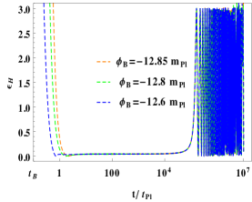
First, we numerically evolve Tβˆ’m​o​d​e​lπ‘‡π‘šπ‘œπ‘‘π‘’π‘™T-model with the background given by Eqs.(1) and (3) for Ξ±=10​mP​l2𝛼10superscriptsubscriptπ‘šπ‘ƒπ‘™2\alpha=10m_{Pl}^{2}. The results for a set of KED initial conditions at the bounce are presented in Fig. 2, in which the scale factor a​(t)π‘Žπ‘‘a(t), the EoS w​(Ο•)𝑀italic-Ο•w(\phi) and the slow-roll parameter Ο΅Hsubscriptitalic-ϡ𝐻\epsilon_{H} are shown for the same set of Ο•Bsubscriptitalic-ϕ𝐡\phi_{B}. In the future evolution of w​(Ο•)𝑀italic-Ο•w(\phi) and Ο΅Hsubscriptitalic-ϡ𝐻\epsilon_{H}, we obtain inflationary and non-inflationary phases. This means, in the entire parameter space of the KED initial conditions, we also have a small subset that does not provide inflationary phase, see Fig. 2 and Table 2.

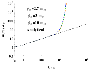
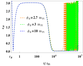
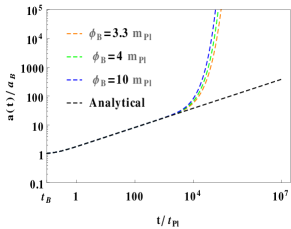
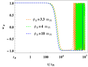
From the top panels of Fig. 2, one can clearly see that the desired slow-roll inflationary phase is obtained for the chosen initial values of Ο•B/mP​l=βˆ’5,4,10subscriptitalic-ϕ𝐡subscriptπ‘šπ‘ƒπ‘™5410\phi_{B}/m_{Pl}=-5,4,10. In this region, a​(t)π‘Žπ‘‘a(t) grows exponentially, w​(Ο•)β‰ƒβˆ’1similar-to-or-equals𝑀italic-Ο•1w(\phi)\simeq-1 and Ο΅Hβ‰ͺ1much-less-thansubscriptitalic-ϡ𝐻1\epsilon_{H}\ll 1. For NIV (Ο•Λ™B<0subscriptΛ™italic-ϕ𝐡0\dot{\phi}_{B}<0), one can obtain the same results with the replacement of Ο•Bsubscriptitalic-ϕ𝐡\phi_{B} by βˆ’Ο•Bsubscriptitalic-ϕ𝐡-\phi_{B} [i.e. Ο•B/mP​l=5,βˆ’4,βˆ’10subscriptitalic-ϕ𝐡subscriptπ‘šπ‘ƒπ‘™5410\phi_{B}/m_{Pl}=5,-4,-10].

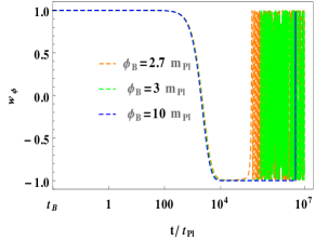
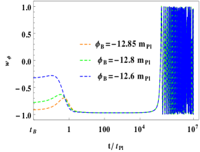
From the curves of w​(Ο•)𝑀italic-Ο•w(\phi) (top panel of Fig. 2), we notice that the evolution of the universe before reheating can be split up into three different phases, namely bouncing, transition and slow-roll alam2017 ; Tao2017a ; Tao2017b . During the bouncing phase, the kinetic energy remains dominant, and w​(Ο•)≃+1similar-to-or-equals𝑀italic-Ο•1w(\phi)\simeq+1. In the transition phase, w​(Ο•)𝑀italic-Ο•w(\phi) decreases drastically from +11+1 (t/tP​l≃103)similar-to-or-equals𝑑subscript𝑑𝑃𝑙superscript103(t/t_{Pl}\simeq 10^{3}) to βˆ’11-1 (t/tP​l≃104)similar-to-or-equals𝑑subscript𝑑𝑃𝑙superscript104(t/t_{Pl}\simeq 10^{4}). This transition phase is slightly short in comparison with the other two phases. In the slow-roll phase, w​(Ο•)𝑀italic-Ο•w(\phi) is close to βˆ’11-1, and remains so until the end of the slow-roll inflation. During the bouncing phase, it is remarkable to note that the evolution of a​(t)π‘Žπ‘‘a(t) (top panel of Fig. 2) is independent for a wide range of initial values of Ο•Bsubscriptitalic-ϕ𝐡\phi_{B}, and exhibits the compatible behavior with the analytical solution (12).

The entire range of KED initial conditions is from βˆ’βˆž-\infty to +∞+\infty. In this range most of initial values provide inflationary phase. However, there is a small subset that does not give inflationary phase, see Table 2. Total number of e𝑒e-folds Ni​n​fsubscript𝑁𝑖𝑛𝑓N_{inf} during the inflationary phase can be obtained for different values of Ο•Bsubscriptitalic-ϕ𝐡\phi_{B}, and the range for Ο•BΛ™>0Λ™subscriptitalic-ϕ𝐡0\dot{\phi_{B}}>0 is given as (See Table 2)

Ο•BmP​l∈(βˆ’βˆž,βˆ’3.1)βˆͺ(βˆ’1.61,+∞)subscriptitalic-ϕ𝐡subscriptπ‘šπ‘ƒπ‘™3.11.61\displaystyle\frac{\phi_{B}}{m_{Pl}}\in(-\infty,-3.1)\cup(-1.61,+\infty)
β†’slow-roll​(Ni​n​f>0),β†’absentslow-rollsubscript𝑁𝑖𝑛𝑓0\displaystyle~{}~{}~{}~{}~{}~{}~{}~{}~{}~{}~{}~{}~{}\rightarrow\text{slow-roll}~{}(N_{inf}>0),
βˆ’3.1<Ο•Bβ‰€βˆ’1.6β†’no slow-roll inflation.3.1subscriptitalic-ϕ𝐡1.6β†’no slow-roll inflation\displaystyle-3.1<\phi_{B}\leq-1.6\rightarrow\text{no slow-roll inflation}. (22)

To be consistent with the Planck data Planck2015 , at least 60 e𝑒e-folds are needed during the slow-roll inflation, and to obtain it one has to require (see Table 3)

Ο•BmP​lsubscriptitalic-ϕ𝐡subscriptπ‘šπ‘ƒπ‘™\displaystyle\frac{\phi_{B}}{m_{Pl}} ∈\displaystyle\in (βˆ’βˆž,βˆ’4.9)βˆͺ(1.1,+∞).4.91.1\displaystyle(-\infty,-4.9)\cup(1.1,+\infty). (23)

In the case of initial conditions with Ο•Λ™B<0subscriptΛ™italic-ϕ𝐡0\dot{\phi}_{B}<0, we use the symmetry (Ο•B,Ο•Λ™B)β†’(βˆ’Ο•B,βˆ’Ο•Λ™B)β†’subscriptitalic-ϕ𝐡subscriptΛ™italic-ϕ𝐡subscriptitalic-ϕ𝐡subscriptΛ™italic-ϕ𝐡(\phi_{B},\dot{\phi}_{B})\rightarrow(-\phi_{B},-\dot{\phi}_{B}), then the constraints are

Ο•BmP​lsubscriptitalic-ϕ𝐡subscriptπ‘šπ‘ƒπ‘™\displaystyle\frac{\phi_{B}}{m_{Pl}} ∈\displaystyle\in (βˆ’βˆž,1.61)βˆͺ(3.1,+∞)β†’slow-roll​(Ni​n​f>0)β†’1.613.1slow-rollsubscript𝑁𝑖𝑛𝑓0\displaystyle(-\infty,1.61)\cup(3.1,+\infty)\rightarrow\text{slow-roll}~{}(N_{inf}>0)
1.6≀ϕB<3.1β†’no slow-roll,1.6subscriptitalic-ϕ𝐡3.1β†’no slow-roll\displaystyle 1.6\leq\phi_{B}<3.1\rightarrow\text{no slow-roll},
Ο•BmP​lsubscriptitalic-ϕ𝐡subscriptπ‘šπ‘ƒπ‘™\displaystyle\frac{\phi_{B}}{m_{Pl}} ∈\displaystyle\in (βˆ’βˆž,βˆ’1.1)βˆͺ(4.9,+∞)β†’Ni​n​f≳60.β†’1.14.9subscript𝑁𝑖𝑛𝑓greater-than-or-equivalent-to60\displaystyle(-\infty,-1.1)\cup(4.9,+\infty)\rightarrow N_{inf}\gtrsim 60. (24)

From Table 3, one notices that the number of e𝑒e-folds Ni​n​fsubscript𝑁𝑖𝑛𝑓N_{inf} grows as the absolute values of Ο•Bsubscriptitalic-ϕ𝐡\phi_{B} increase, which implies that an absolute large value of Ο•Bsubscriptitalic-ϕ𝐡\phi_{B} can produce more number of e𝑒e-folds. The similar results for power-law potentials were obtained in alam2017 .

Next, we study Tβˆ’m​o​d​e​lπ‘‡π‘šπ‘œπ‘‘π‘’π‘™T-model with Ξ±=1010​mP​l2𝛼superscript1010superscriptsubscriptπ‘šπ‘ƒπ‘™2\alpha=10^{10}m_{Pl}^{2}. The results are displayed in Fig. 3 for Ο•Λ™B>0subscriptΛ™italic-ϕ𝐡0\dot{\phi}_{B}>0. Here, we use a large value of α𝛼\alpha to get both KED and PED initial conditions at the quantum bounce. In Fig. 3, we show the evolution of the scale factor a​(t)π‘Žπ‘‘a(t), EoS w​(Ο•)𝑀italic-Ο•w(\phi) and slow-roll parameter Ο΅Hsubscriptitalic-ϡ𝐻\epsilon_{H}, and show the inflationary and non-inflationary phases of the universe. Top, middle and bottom panels of Fig. 3 are obtained for the different sets of initial conditions of Ο•Bsubscriptitalic-ϕ𝐡\phi_{B} that correspond to KED with slow-roll (Top), without slow-roll (Middle) and PED with slow-roll (Bottom). From the top and middle panels of Fig. 3, we conclude that the KED initial conditions have a subset that does not provide slow-roll inflation phases. The range of the above subset is given in Table 2.

Let us compare Top and bottom panels of Fig. 3 that are obtained for KED and PED initial conditions. In top panels, the evolution of a​(t)π‘Žπ‘‘a(t) exhibits the universal feature which is consistent with the analytical solution (12). The evolution of w​(Ο•)𝑀italic-Ο•w(\phi) shows three different phases, namely bouncing, transition and slow-roll. In bottom panels, the universal feature of a​(t)π‘Žπ‘‘a(t) is lost, and the bouncing phase no longer exists, though the slow-roll inflation w​(Ο•)β‰ƒβˆ’1similar-to-or-equals𝑀italic-Ο•1w(\phi)\simeq-1 can still be achieved.

The range of Ο•Bsubscriptitalic-ϕ𝐡\phi_{B} that provides inflationary and non-inflationary phases is given by (see Table 2):

Ο•BmP​l∈(βˆ’Ο•m​a​x,βˆ’3.21)βˆͺ(βˆ’1.8,Ο•m​a​x),subscriptitalic-ϕ𝐡subscriptπ‘šπ‘ƒπ‘™subscriptitalic-Ο•π‘šπ‘Žπ‘₯3.211.8subscriptitalic-Ο•π‘šπ‘Žπ‘₯\displaystyle\frac{\phi_{B}}{m_{Pl}}\in(-\phi_{max},-3.21)\cup(-1.8,\phi_{max}),
β†’slow-roll​(Ni​n​f>0),β†’absentslow-rollsubscript𝑁𝑖𝑛𝑓0\displaystyle~{}~{}~{}~{}~{}~{}~{}~{}~{}~{}~{}~{}~{}\rightarrow\text{slow-roll}~{}(N_{inf}>0),
βˆ’3.2≀ϕB<βˆ’1.8β†’no slow-roll inflation,3.2subscriptitalic-ϕ𝐡1.8β†’no slow-roll inflation,\displaystyle-3.2\leq\phi_{B}<-1.8\rightarrow\text{no slow-roll inflation,} (25)

where

Ο•m​a​x≃6​α​arctan⁑h​(ρcα​c2)≃2.56Γ—105​mP​l.similar-to-or-equalssubscriptitalic-Ο•π‘šπ‘Žπ‘₯6𝛼hsubscriptπœŒπ‘π›Όsuperscript𝑐2similar-to-or-equals2.56superscript105subscriptπ‘šπ‘ƒπ‘™\displaystyle\phi_{max}\simeq\sqrt{6\alpha}\arctan\text{h}\left(\sqrt{\frac{\rho_{c}}{\alpha c^{2}}}\right)\simeq 2.56\times 10^{5}m_{Pl}. (26)

To obtain at least 60 e𝑒e-folds during the slow-roll inflationary phase, one has to require (see Table 3):

Ο•BmP​l∈(βˆ’Ο•m​a​x,βˆ’5.1)βˆͺ(1.05,Ο•m​a​x).subscriptitalic-ϕ𝐡subscriptπ‘šπ‘ƒπ‘™subscriptitalic-Ο•π‘šπ‘Žπ‘₯5.11.05subscriptitalic-Ο•π‘šπ‘Žπ‘₯\displaystyle\frac{\phi_{B}}{m_{Pl}}\in(-\phi_{max},-5.1)\cup(1.05,\phi_{max}). (27)

For Ο•Λ™B<0subscriptΛ™italic-ϕ𝐡0\dot{\phi}_{B}<0, the same results can be obtained with the symmetry (Ο•B,Ο•Λ™B)β†’(βˆ’Ο•B,βˆ’Ο•Λ™B)β†’subscriptitalic-ϕ𝐡subscriptΛ™italic-ϕ𝐡subscriptitalic-ϕ𝐡subscriptΛ™italic-ϕ𝐡(\phi_{B},\dot{\phi}_{B})\rightarrow(-\phi_{B},-\dot{\phi}_{B}), and are given by

Ο•BmP​l∈(βˆ’Ο•m​a​x,1.8)βˆͺ(3.21,Ο•m​a​x),subscriptitalic-ϕ𝐡subscriptπ‘šπ‘ƒπ‘™subscriptitalic-Ο•π‘šπ‘Žπ‘₯1.83.21subscriptitalic-Ο•π‘šπ‘Žπ‘₯\displaystyle\frac{\phi_{B}}{m_{Pl}}\in(-\phi_{max},1.8)\cup(3.21,\phi_{max}),
β†’slow-roll​(Ni​n​f>0)β†’absentslow-rollsubscript𝑁𝑖𝑛𝑓0\displaystyle~{}~{}~{}~{}~{}~{}~{}~{}~{}~{}~{}~{}\rightarrow\text{slow-roll}~{}(N_{inf}>0)
1.8<Ο•B≀3.2β†’no slow-roll,1.8subscriptitalic-ϕ𝐡3.2β†’no slow-roll\displaystyle 1.8<\phi_{B}\leq 3.2\rightarrow\text{no slow-roll},
Ο•BmP​l∈(βˆ’Ο•m​a​x,βˆ’1.05)βˆͺ(5.1,Ο•m​a​x)subscriptitalic-ϕ𝐡subscriptπ‘šπ‘ƒπ‘™subscriptitalic-Ο•π‘šπ‘Žπ‘₯1.055.1subscriptitalic-Ο•π‘šπ‘Žπ‘₯\displaystyle\frac{\phi_{B}}{m_{Pl}}\in(-\phi_{max},-1.05)\cup(5.1,\phi_{max})
β†’Ni​n​f≳60.β†’absentsubscript𝑁𝑖𝑛𝑓greater-than-or-equivalent-to60\displaystyle~{}~{}~{}~{}~{}~{}~{}~{}~{}~{}\rightarrow N_{inf}\gtrsim 60. (28)

As mentioned in the case of Ξ±=10​mP​l2𝛼10superscriptsubscriptπ‘šπ‘ƒπ‘™2\alpha=10m_{Pl}^{2}, here also one can get more e-folds for the large absolute values of Ο•Bsubscriptitalic-ϕ𝐡\phi_{B}, see Table 3.

Table 4: This table represents the Eβˆ’m​o​d​e​lπΈπ‘šπ‘œπ‘‘π‘’π‘™E-model. We show the number of e𝑒e-foldings Ni​n​fsubscript𝑁𝑖𝑛𝑓N_{inf} and other parameters with Ο•Λ™B>0subscriptΛ™italic-ϕ𝐡0\dot{\phi}_{B}>0. For each choice of α𝛼\alpha, the corresponding values of c𝑐c are given by Eq.(19).
α𝛼\alpha Ο•Bsubscriptitalic-ϕ𝐡\phi_{B} Inflation t/tp​l𝑑subscript𝑑𝑝𝑙t/t_{pl} Ο΅italic-Ο΅\epsilon w𝑀w Ni​n​fsubscript𝑁𝑖𝑛𝑓N_{inf} Β Β Β rwc/rwsuperscriptsubscriptπ‘Ÿπ‘€π‘subscriptπ‘Ÿπ‘€r_{w}^{c}/r_{w} Β Β Β wBsuperscript𝑀𝐡{w}^{B}
0.1 βˆ’0.50.5-0.5 begin 2.65082Γ—1032.65082superscript1032.65082\times 10^{3} 0.99 βˆ’1/313-1/3
slow-roll 1.10225Γ—1041.10225superscript1041.10225\times 10^{4} 1.0Γ—10βˆ’41.0superscript1041.0\times 10^{-4} βˆ’11-1 42.77 rwc>rwsuperscriptsubscriptπ‘Ÿπ‘€π‘subscriptπ‘Ÿπ‘€r_{w}^{c}>r_{w} >0absent0>0
end 3.243Γ—1053.243superscript1053.243\times 10^{5} 0.99 βˆ’1/313-1/3
βˆ’0.380.38-0.38 begin 2.62043Γ—1032.62043superscript1032.62043\times 10^{3} 0.99 βˆ’1/313-1/3
slow-roll 1.16211Γ—1041.16211superscript1041.16211\times 10^{4} 1.8Γ—10βˆ’41.8superscript1041.8\times 10^{-4} βˆ’11-1 60.0 rwc=rwsuperscriptsubscriptπ‘Ÿπ‘€π‘subscriptπ‘Ÿπ‘€r_{w}^{c}=r_{w} >0absent0>0
end 4.425Γ—1054.425superscript1054.425\times 10^{5} 0.99 βˆ’1/313-1/3
βˆ’0.30.3-0.3 begin 2.60392Γ—1032.60392superscript1032.60392\times 10^{3} 0.99 βˆ’1/313-1/3
slow-roll 1.20318Γ—1041.20318superscript1041.20318\times 10^{4} 2.4Γ—10βˆ’42.4superscript1042.4\times 10^{-4} βˆ’11-1 74.92 rwc<rwsuperscriptsubscriptπ‘Ÿπ‘€π‘subscriptπ‘Ÿπ‘€r_{w}^{c}<r_{w} >0absent0>0
end 5.441Γ—1065.441superscript1065.441\times 10^{6} 0.99 βˆ’1/313-1/3
5 βˆ’2525-25 begin 0.30.30.3 1.5 βˆ’0.4780.478-0.478
slow-roll 1.51.51.5 1.3Γ—10βˆ’31.3superscript1031.3\times 10^{-3} βˆ’0.9780.978-0.978 713.22 rwc<rwsuperscriptsubscriptπ‘Ÿπ‘€π‘subscriptπ‘Ÿπ‘€r_{w}^{c}<r_{w} <0absent0<0
end 2.963Γ—1052.963superscript1052.963\times 10^{5} 0.31 βˆ’1/313-1/3
βˆ’66-6 begin 5.6861Γ—1025.6861superscript1025.6861\times 10^{2} 0.99 βˆ’1/313-1/3
slow-roll 3.0Γ—1033.0superscript1033.0\times 10^{3} 1.8Γ—10βˆ’21.8superscript1021.8\times 10^{-2} βˆ’0.9870.987-0.987 79.14 rwc<rwsuperscriptsubscriptπ‘Ÿπ‘€π‘subscriptπ‘Ÿπ‘€r_{w}^{c}<r_{w} >0absent0>0
end 4.4Γ—1054.4superscript1054.4\times 10^{5} 0.99 βˆ’1/313-1/3
βˆ’5.355.35-5.35 begin 7.8972Γ—1027.8972superscript1027.8972\times 10^{2} 0.99 βˆ’1/313-1/3
slow-roll 6.78678Γ—1036.78678superscript1036.78678\times 10^{3} 2.0Γ—10βˆ’22.0superscript1022.0\times 10^{-2} βˆ’0.9870.987-0.987 60.28 rwc=rwsuperscriptsubscriptπ‘Ÿπ‘€π‘subscriptπ‘Ÿπ‘€r_{w}^{c}=r_{w} >0absent0>0
end 4.07Γ—1054.07superscript1054.07\times 10^{5} 1.0 βˆ’1/313-1/3
βˆ’55-5 begin 9.5418Γ—1029.5418superscript1029.5418\times 10^{2} 0.99 βˆ’1/313-1/3
slow-roll 9.55025Γ—1039.55025superscript1039.55025\times 10^{3} 2.1Γ—10βˆ’22.1superscript1022.1\times 10^{-2} βˆ’0.9850.985-0.985 50.69 rwc>rwsuperscriptsubscriptπ‘Ÿπ‘€π‘subscriptπ‘Ÿπ‘€r_{w}^{c}>r_{w} >0absent0>0
end 3.85Γ—1053.85superscript1053.85\times 10^{5} 1.0 βˆ’1/313-1/3
0.50.50.5 begin 4.26416Γ—1034.26416superscript1034.26416\times 10^{3} 0.99 βˆ’1/313-1/3
slow-roll 1.43245Γ—1041.43245superscript1041.43245\times 10^{4} 2.7Γ—10βˆ’42.7superscript1042.7\times 10^{-4} βˆ’11-1 47.83 rwc>rwsuperscriptsubscriptπ‘Ÿπ‘€π‘subscriptπ‘Ÿπ‘€r_{w}^{c}>r_{w} >0absent0>0
end 7.85Γ—1057.85superscript1057.85\times 10^{5} 0.99 βˆ’1/313-1/3
0.760.760.76 begin 3.99721Γ—1033.99721superscript1033.99721\times 10^{3} 1.0 βˆ’1/313-1/3
slow-roll 1.39402Γ—1041.39402superscript1041.39402\times 10^{4} 1.0Γ—10βˆ’41.0superscript1041.0\times 10^{-4} βˆ’11-1 60.45 rwc=rwsuperscriptsubscriptπ‘Ÿπ‘€π‘subscriptπ‘Ÿπ‘€r_{w}^{c}=r_{w} >0absent0>0
end 9.19Γ—1059.19superscript1059.19\times 10^{5} 0.99 βˆ’1/313-1/3
111 begin 3.79512Γ—1033.79512superscript1033.79512\times 10^{3} 0.99 βˆ’1/313-1/3
slow-roll 1.36658Γ—1041.36658superscript1041.36658\times 10^{4} 3.6Γ—10βˆ’43.6superscript1043.6\times 10^{-4} βˆ’11-1 73.96 rwc<rwsuperscriptsubscriptπ‘Ÿπ‘€π‘subscriptπ‘Ÿπ‘€r_{w}^{c}<r_{w} >0absent0>0
end 1.054Γ—1061.054superscript1061.054\times 10^{6} 0.99 βˆ’1/313-1/3
Table 5: This table is for the Eβˆ’m​o​d​e​lπΈπ‘šπ‘œπ‘‘π‘’π‘™E-model. We exhibit different parameters with Ο•Λ™B<0subscriptΛ™italic-ϕ𝐡0\dot{\phi}_{B}<0.
α𝛼\alpha Ο•Bsubscriptitalic-ϕ𝐡\phi_{B} Inflation t/tp​l𝑑subscript𝑑𝑝𝑙t/t_{pl} Ο΅italic-Ο΅\epsilon w𝑀w Ni​n​fsubscript𝑁𝑖𝑛𝑓N_{inf} Β Β Β rwc/rwsuperscriptsubscriptπ‘Ÿπ‘€π‘subscriptπ‘Ÿπ‘€r_{w}^{c}/r_{w} Β Β Β wBsuperscript𝑀𝐡{w}^{B}
0.1 333 begin 2.62892Γ—1032.62892superscript1032.62892\times 10^{3} 0.99 βˆ’1/313-1/3
slow-roll 2.56475Γ—1042.56475superscript1042.56475\times 10^{4} 1.6Γ—10βˆ’31.6superscript1031.6\times 10^{-3} βˆ’0.9990.999-0.999 39.16 rwc>rwsuperscriptsubscriptπ‘Ÿπ‘€π‘subscriptπ‘Ÿπ‘€r_{w}^{c}>r_{w} >0absent0>0
end 2.992Γ—1052.992superscript1052.992\times 10^{5} 0.99 βˆ’1/313-1/3
3.15 begin 2.59873Γ—1032.59873superscript1032.59873\times 10^{3} 0.99 βˆ’1/313-1/3
slow-roll 2.50846Γ—1042.50846superscript1042.50846\times 10^{4} 3.4Γ—10βˆ’53.4superscript1053.4\times 10^{-5} βˆ’0.9990.999-0.999 60.48 rwc=rwsuperscriptsubscriptπ‘Ÿπ‘€π‘subscriptπ‘Ÿπ‘€r_{w}^{c}=r_{w} >0absent0>0
end 4.457Γ—1054.457superscript1054.457\times 10^{5} 0.99 βˆ’1/313-1/3
3.3 begin 2.57866Γ—1032.57866superscript1032.57866\times 10^{3} 0.99 βˆ’1/313-1/3
slow-roll 2.50846Γ—1042.50846superscript1042.50846\times 10^{4} 1.1Γ—10βˆ’31.1superscript1031.1\times 10^{-3} βˆ’0.9990.999-0.999 92.19 rwc<rwsuperscriptsubscriptπ‘Ÿπ‘€π‘subscriptπ‘Ÿπ‘€r_{w}^{c}<r_{w} >0absent0>0
end 6.611Γ—1056.611superscript1056.611\times 10^{5} 0.99 βˆ’1/313-1/3
5 βˆ’2525-25 begin 0.20.20.2 4.94 βˆ’0.5070.507-0.507
slow-roll 0.80.80.8 1.1Γ—10βˆ’21.1superscript1021.1\times 10^{-2} βˆ’0.9950.995-0.995 712.15 rwc<rwsuperscriptsubscriptπ‘Ÿπ‘€π‘subscriptπ‘Ÿπ‘€r_{w}^{c}<r_{w} <0absent0<0
end 2.47527Γ—1052.47527superscript1052.47527\times 10^{5} 0.28 βˆ’1/313-1/3
βˆ’33-3 begin 5.88967Γ—1025.88967superscript1025.88967\times 10^{2} 0.99 βˆ’1/313-1/3
slow-roll 1.74169Γ—1031.74169superscript1031.74169\times 10^{3} 6.6Γ—10βˆ’56.6superscript1056.6\times 10^{-5} βˆ’11-1 80.19 rwc<rwsuperscriptsubscriptπ‘Ÿπ‘€π‘subscriptπ‘Ÿπ‘€r_{w}^{c}<r_{w} >0absent0>0
end 4.42Γ—1054.42superscript1054.42\times 10^{5} 1.0 βˆ’1/313-1/3
βˆ’2.22.2-2.2 begin 8.361Γ—1028.361superscript1028.361\times 10^{2} 0.99 βˆ’1/313-1/3
slow-roll 2.42178Γ—1032.42178superscript1032.42178\times 10^{3} 9.5Γ—10βˆ’59.5superscript1059.5\times 10^{-5} βˆ’11-1 60.23 rwc=rwsuperscriptsubscriptπ‘Ÿπ‘€π‘subscriptπ‘Ÿπ‘€r_{w}^{c}=r_{w} >0absent0>0
end 4.07Γ—1054.07superscript1054.07\times 10^{5} 1.0 βˆ’1/313-1/3
βˆ’22-2 begin 9.1693Γ—1029.1693superscript1029.1693\times 10^{2} 0.99 βˆ’1/313-1/3
slow-roll 2.6382Γ—1032.6382superscript1032.6382\times 10^{3} 3.3Γ—10βˆ’63.3superscript1063.3\times 10^{-6} βˆ’11-1 55.51 rwc>rwsuperscriptsubscriptπ‘Ÿπ‘€π‘subscriptπ‘Ÿπ‘€r_{w}^{c}>r_{w} >0absent0>0
end 3.966Γ—1053.966superscript1053.966\times 10^{5} 1.0 βˆ’1/313-1/3
4.2 begin 4.11346Γ—1034.11346superscript1034.11346\times 10^{3} 0.99 βˆ’1/313-1/3
slow-roll 3.77015Γ—1043.77015superscript1043.77015\times 10^{4} 6.2Γ—10βˆ’36.2superscript1036.2\times 10^{-3} βˆ’0.9950.995-0.995 48.70 rwc>rwsuperscriptsubscriptπ‘Ÿπ‘€π‘subscriptπ‘Ÿπ‘€r_{w}^{c}>r_{w} >0absent0>0
end 7.944Γ—1057.944superscript1057.944\times 10^{5} 0.99 βˆ’1/313-1/3
4.424.424.42 begin 3.89349Γ—1033.89349superscript1033.89349\times 10^{3} 0.99 βˆ’1/313-1/3
slow-roll 5.83076Γ—1045.83076superscript1045.83076\times 10^{4} 3.8Γ—10βˆ’33.8superscript1033.8\times 10^{-3} βˆ’0.9960.996-0.996 60.33 rwc=rwsuperscriptsubscriptπ‘Ÿπ‘€π‘subscriptπ‘Ÿπ‘€r_{w}^{c}=r_{w} >0absent0>0
end 9.173Γ—1059.173superscript1059.173\times 10^{5} 0.99 βˆ’1/313-1/3
5 begin 3.47442Γ—1033.47442superscript1033.47442\times 10^{3} 0.99 βˆ’1/313-1/3
slow-roll 3.27722Γ—1043.27722superscript1043.27722\times 10^{4} 2.3Γ—10βˆ’32.3superscript1032.3\times 10^{-3} βˆ’0.9980.998-0.998 99.13 rwc<rwsuperscriptsubscriptπ‘Ÿπ‘€π‘subscriptπ‘Ÿπ‘€r_{w}^{c}<r_{w} >0absent0>0
end 1.292Γ—1061.292superscript1061.292\times 10^{6} 0.99 βˆ’1/313-1/3

Finally, we consider the evolutions of the kinetic and potential energies in Fig. 4, and pay particular attention on the case in which a slow-roll inflationary phase is absent, although the kinetic energy of the inflaton still dominates the evolution of the universe at the bounce. Left panel is plotted for KED initial condition with Ο•B=5​mP​lsubscriptitalic-ϕ𝐡5subscriptπ‘šπ‘ƒπ‘™\phi_{B}=5m_{Pl}. In the bouncing phase, KE dominates the evolution whereas PE remains sub-dominant. As time increases, KE decreases until the transition phase in which KE falls below the PE, and thereafter, PE dominates and remains so for most of the time of the evolution, during which the slow-roll inflation is resulted. Middle panel is shown for a value (Ο•B=βˆ’2.4​mP​lsubscriptitalic-ϕ𝐡2.4subscriptπ‘šπ‘ƒπ‘™\phi_{B}=-2.4m_{Pl}) of a subset of KED initial conditions. In this case, PE is sub-dominant initially and remains so during the entire evolution. It never overtakes the KE. As a result, a slow-roll inflationary phase is absent. Right panel exhibits the PED case where PE dominates generically during the whole process, and gives rise to a slow-roll inflationary phase for a long period.

III.2 E-model

In this subsection, we study the features of Eβˆ’m​o​d​e​lπΈπ‘šπ‘œπ‘‘π‘’π‘™E-model [Eq.(18)]. The Eβˆ’m​o​d​e​lπΈπ‘šπ‘œπ‘‘π‘’π‘™E-model potential is displayed in Fig. 1. This kind of potentials is bounded below by zero i.e. V​(Ο•)β‰₯0𝑉italic-Ο•0V(\phi)\geq 0. On the positive side (Ο•β†’βˆžβ†’italic-Ο•\phi\rightarrow\infty), the potential (18) achieves a finite value V​(Ο•)→α​c2/4→𝑉italic-ϕ𝛼superscript𝑐24V(\phi)\rightarrow\alpha c^{2}/4, whereas in the negative side (Ο•β†’βˆ’βˆžβ†’italic-Ο•\phi\rightarrow-\infty) it diverges. Hence, this potential is asymmetric. In LQC, the total energy density can not exceed the value of ρcsubscriptπœŒπ‘\rho_{c}. Therefore, the critical energy density constrains the initial values of Ο•Bsubscriptitalic-ϕ𝐡\phi_{B} as (Ο•m​i​n,∞)subscriptitalic-Ο•π‘šπ‘–π‘›(\phi_{min},\infty), where

Ο•m​i​nsubscriptitalic-Ο•π‘šπ‘–π‘›\displaystyle\phi_{min} ≃similar-to-or-equals\displaystyle\simeq 6​α​arctan⁑h​(ρcα​c2βˆ’Οc)6𝛼hsubscriptπœŒπ‘π›Όsuperscript𝑐2subscriptπœŒπ‘\displaystyle\sqrt{6\alpha}\arctan\text{h}\left(\frac{\sqrt{\rho_{c}}}{\sqrt{\alpha c^{2}}-\sqrt{\rho_{c}}}\right) (29)
≃similar-to-or-equals\displaystyle\simeq βˆ’3.64​mP​l​for​α=0.1​mP​l2,3.64subscriptπ‘šπ‘ƒπ‘™for𝛼0.1superscriptsubscriptπ‘šπ‘ƒπ‘™2\displaystyle-3.64m_{Pl}~{}\text{for}~{}\alpha=0.1m_{Pl}^{2},
≃similar-to-or-equals\displaystyle\simeq βˆ’25.65​mP​l​for​α=5​mP​l2.25.65subscriptπ‘šπ‘ƒπ‘™for𝛼5superscriptsubscriptπ‘šπ‘ƒπ‘™2\displaystyle-25.65m_{Pl}~{}\text{for}~{}\alpha=5m_{Pl}^{2}.

The Eβˆ’m​o​d​e​lπΈπ‘šπ‘œπ‘‘π‘’π‘™E-model reduces to the Starobinsky model for Ξ±=1𝛼1\alpha=1. Here, we shall not discuss the Starobinsky model as the evolutions and the phase space analysis have been already studied in detail in Tao2017a ; Tao2017b ; Bonga2016 . Hence, in this sub-section, we shall investigate Eβˆ’m​o​d​e​lπΈπ‘šπ‘œπ‘‘π‘’π‘™E-model with different values of α𝛼\alpha (Ξ±β‰ 1𝛼1\alpha\not=1).

From Eq.(29), one can obtain Ο•m​i​nsubscriptitalic-Ο•π‘šπ‘–π‘›\phi_{min} for the given value of α𝛼\alpha and c𝑐c. First, let us work with Ξ±=0.1​mP​l2𝛼0.1superscriptsubscriptπ‘šπ‘ƒπ‘™2\alpha=0.1m_{Pl}^{2} and c=3.3Γ—10βˆ’4​mP​l𝑐3.3superscript104subscriptπ‘šπ‘ƒπ‘™c=3.3\times 10^{-4}m_{Pl} [Eq.(19)]. In this case, we have Ο•m​i​nβ‰ƒβˆ’3.64​mP​lsimilar-to-or-equalssubscriptitalic-Ο•π‘šπ‘–π‘›3.64subscriptπ‘šπ‘ƒπ‘™\phi_{min}\simeq-3.64m_{Pl}. Numerically, we examine the whole range of the inflaton field in order to identify the initial conditions that can give rise to the slow-roll inflation. We find the KED (PED) evolution exists in a very long (narrow) range and given by (see, Table 2):

βˆ™βˆ™\bullet For Ο•Λ™B>0subscriptΛ™italic-ϕ𝐡0\dot{\phi}_{B}>0, we have

Ο•BmP​l∈(βˆ’1.51,+∞)β†’KED (SR),subscriptitalic-ϕ𝐡subscriptπ‘šπ‘ƒπ‘™1.51β†’KED (SR)\displaystyle\frac{\phi_{B}}{m_{Pl}}\in(-1.51,+\infty)\rightarrow\text{KED (SR)},
βˆ’3.52<Ο•Bβ‰€βˆ’1.5β†’subset of KED (NSR),3.52subscriptitalic-ϕ𝐡1.5β†’subset of KED (NSR)\displaystyle-3.52<\phi_{B}\leq-1.5\rightarrow\text{subset of KED (NSR)},
Ο•BmP​l=βˆ’3.52β†’KED=PED (NSR),subscriptitalic-ϕ𝐡subscriptπ‘šπ‘ƒπ‘™3.52β†’KED=PED (NSR)\displaystyle\frac{\phi_{B}}{m_{Pl}}=-3.52\rightarrow\text{KED=PED (NSR)},
Ο•BmP​l∈(Ο•m​i​n,βˆ’3.53)β†’PED (NSR),subscriptitalic-ϕ𝐡subscriptπ‘šπ‘ƒπ‘™subscriptitalic-Ο•π‘šπ‘–π‘›3.53β†’PED (NSR)\displaystyle\frac{\phi_{B}}{m_{Pl}}\in(\phi_{min},-3.53)\rightarrow\text{PED (NSR)}, (30)

where Ο•m​i​nsubscriptitalic-Ο•π‘šπ‘–π‘›\phi_{min} is given by Eq.(29).

βˆ™βˆ™\bullet For Ο•Λ™B<0subscriptΛ™italic-ϕ𝐡0\dot{\phi}_{B}<0, we obtain

Ο•BmP​l∈(2.4,+∞)β†’KED (SR),subscriptitalic-ϕ𝐡subscriptπ‘šπ‘ƒπ‘™2.4β†’KED (SR)\displaystyle\frac{\phi_{B}}{m_{Pl}}\in(2.4,+\infty)\rightarrow\text{KED (SR)},
βˆ’3.51<Ο•B<2.4β†’subset of KED (NSR),3.51subscriptitalic-ϕ𝐡2.4β†’subset of KED (NSR)\displaystyle-3.51<\phi_{B}<2.4\rightarrow\text{subset of KED (NSR)},
Ο•BmP​l=βˆ’3.51β†’KED=PED (NSR),subscriptitalic-ϕ𝐡subscriptπ‘šπ‘ƒπ‘™3.51β†’KED=PED (NSR)\displaystyle\frac{\phi_{B}}{m_{Pl}}=-3.51\rightarrow\text{KED=PED (NSR)},
Ο•BmP​l∈(Ο•m​i​n,βˆ’3.52)β†’PED (NSR).subscriptitalic-ϕ𝐡subscriptπ‘šπ‘ƒπ‘™subscriptitalic-Ο•π‘šπ‘–π‘›3.52β†’PED (NSR)\displaystyle\frac{\phi_{B}}{m_{Pl}}\in(\phi_{min},-3.52)\rightarrow\text{PED (NSR)}. (31)

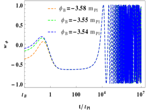
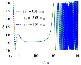
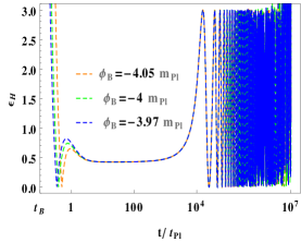
The results of the background evolution for KED and PED initial conditions are shown in Figs. 5 and 6, with Ο•Λ™B>0subscriptΛ™italic-ϕ𝐡0\dot{\phi}_{B}>0 and Ο•Λ™B<0subscriptΛ™italic-ϕ𝐡0\dot{\phi}_{B}<0, respectively. In both figures, the evolutions of a​(t)π‘Žπ‘‘a(t), w​(Ο•)𝑀italic-Ο•w(\phi) and Ο΅Hsubscriptitalic-ϡ𝐻\epsilon_{H} are obtained numerically for the same set of the initial values of Ο•Bsubscriptitalic-ϕ𝐡\phi_{B}. In the case of KED initial conditions, the evolution of a​(t)π‘Žπ‘‘a(t) is universal during the bouncing phase as it does not depends on the form of the potentials nor on the initial values of Ο•Bsubscriptitalic-ϕ𝐡\phi_{B}, and can be well approximated by the analytical solution (12). This is mainly due to the fact that the potential remains very small in comparison with the kinetic one during the whole bouncing phase, and its effects on the evolution of the background is almost negligible. From the evolution of w​(Ο•)𝑀italic-Ο•w(\phi), one can see that the background evolution is divided into three different phases: bouncing, transition and slow-roll. The period of transition phase is very small in comparison with the other two. In the bouncing phase, w​(Ο•)≃+1similar-to-or-equals𝑀italic-Ο•1w(\phi)\simeq+1, while in the transition phase it suddenly decreases from +1​(t/tP​lβ‰ˆ103)1𝑑subscript𝑑𝑃𝑙superscript103+1~{}(t/t_{Pl}\approx 10^{3}) to βˆ’1​(t/tP​lβ‰ˆ104)1𝑑subscript𝑑𝑃𝑙superscript104-1~{}(t/t_{Pl}\approx 10^{4}). In the slow-roll inflationary phase, it is very close to βˆ’11-1 until the end of the slow-roll inflation. In the KED case, we also have a subset that does not provide the slow-roll inflation, which is shown clearly in the middle panels of Figs. 5 and 6. The range of this subset is presented in Table 2. In the case of PED initial conditions, the universality of the scale factor a​(t)π‘Žπ‘‘a(t) is lost, and the bouncing phase does not exist any more, and the slow-roll inflationary phase can not be obtained. See the bottom panels of Figs. 5 and 6.

In Tables 4 and 5, we display the initial values of Ο•Bsubscriptitalic-ϕ𝐡\phi_{B} that provide the desired slow-roll inflation, from which one can see that, for the successful inflation at least 60 e𝑒e-folds are needed and to obtain this, the values of Ο•Bsubscriptitalic-ϕ𝐡\phi_{B} should be in the range of

Ο•BmP​l∈(βˆ’0.38,+∞)β†’Ni​n​f≳60​for​ϕ˙B>0,subscriptitalic-ϕ𝐡subscriptπ‘šπ‘ƒπ‘™0.38β†’subscript𝑁𝑖𝑛𝑓greater-than-or-equivalent-to60forsubscriptΛ™italic-ϕ𝐡0\displaystyle\frac{\phi_{B}}{m_{Pl}}\in(-0.38,+\infty)\rightarrow N_{inf}\gtrsim 60~{}\text{for}~{}\dot{\phi}_{B}>0,
Ο•BmP​l∈(3.15,+∞)β†’Ni​n​f≳60​for​ϕ˙B<0,subscriptitalic-ϕ𝐡subscriptπ‘šπ‘ƒπ‘™3.15β†’subscript𝑁𝑖𝑛𝑓greater-than-or-equivalent-to60forsubscriptΛ™italic-ϕ𝐡0\displaystyle\frac{\phi_{B}}{m_{Pl}}\in(3.15,+\infty)\rightarrow N_{inf}\gtrsim 60~{}\text{for}~{}\dot{\phi}_{B}<0, (32)

within which, Tables 4 and 5 exhibit that Ni​n​fsubscript𝑁𝑖𝑛𝑓N_{inf} grows as Ο•Bsubscriptitalic-ϕ𝐡\phi_{B} increases.

Next, we work with Ξ±=5​mP​l2𝛼5superscriptsubscriptπ‘šπ‘ƒπ‘™2\alpha=5m_{Pl}^{2} and c=4.9Γ—10βˆ’5​mP​l𝑐4.9superscript105subscriptπ‘šπ‘ƒπ‘™c=4.9\times 10^{-5}m_{Pl} [Eq.(19)]. In this case, Ο•m​i​nβ‰ƒβˆ’25.65​mP​lsimilar-to-or-equalssubscriptitalic-Ο•π‘šπ‘–π‘›25.65subscriptπ‘šπ‘ƒπ‘™\phi_{min}\simeq-25.65m_{Pl}. We numerically search the entire range of Ο•Bsubscriptitalic-ϕ𝐡\phi_{B}, and find the initial values that can lead to the slow-roll inflation. Here, KED (PED) evolution has large (small) range and given by (see, Table 2),

Ο•BmP​l∈(βˆ’24.70,βˆ’3.11)βˆͺ(βˆ’1.4,+∞)β†’KED (SR),subscriptitalic-ϕ𝐡subscriptπ‘šπ‘ƒπ‘™24.703.111.4β†’KED (SR)\displaystyle\frac{\phi_{B}}{m_{Pl}}\in(-24.70,-3.11)\cup(-1.4,+\infty)\rightarrow\text{KED (SR)},
βˆ’3.1≀ϕB<βˆ’1.4β†’subset of KED (NSR),3.1subscriptitalic-ϕ𝐡1.4β†’subset of KED (NSR)\displaystyle-3.1\leq\phi_{B}<-1.4\rightarrow\text{subset of KED (NSR)},
Ο•BmP​l=βˆ’24.71β†’KED=PED (SR),subscriptitalic-ϕ𝐡subscriptπ‘šπ‘ƒπ‘™24.71β†’KED=PED (SR)\displaystyle\frac{\phi_{B}}{m_{Pl}}=-24.71\rightarrow\text{KED=PED (SR)},
Ο•BmP​l∈(Ο•m​i​n,βˆ’24.72)β†’PED (SR),subscriptitalic-ϕ𝐡subscriptπ‘šπ‘ƒπ‘™subscriptitalic-Ο•π‘šπ‘–π‘›24.72β†’PED (SR)\displaystyle\frac{\phi_{B}}{m_{Pl}}\in(\phi_{min},-24.72)\rightarrow\text{PED (SR)}, (33)

for Ο•Λ™B>0subscriptΛ™italic-ϕ𝐡0\dot{\phi}_{B}>0, and

Ο•BmP​l∈(βˆ’24.69,1.4)βˆͺ(3,+∞)β†’KED (SR),subscriptitalic-ϕ𝐡subscriptπ‘šπ‘ƒπ‘™24.691.43β†’KED (SR)\displaystyle\frac{\phi_{B}}{m_{Pl}}\in(-24.69,1.4)\cup(3,+\infty)\rightarrow\text{KED (SR)},
1.4<Ο•B<3β†’subset of KED (NSR),1.4subscriptitalic-ϕ𝐡3β†’subset of KED (NSR)\displaystyle 1.4<\phi_{B}<3\rightarrow\text{subset of KED (NSR)},
Ο•BmP​l=βˆ’24.7β†’KED=PED (SR),subscriptitalic-ϕ𝐡subscriptπ‘šπ‘ƒπ‘™24.7β†’KED=PED (SR)\displaystyle\frac{\phi_{B}}{m_{Pl}}=-24.7\rightarrow\text{KED=PED (SR)},
Ο•BmP​l∈(Ο•m​i​n,βˆ’24.71)β†’PED (SR)subscriptitalic-ϕ𝐡subscriptπ‘šπ‘ƒπ‘™subscriptitalic-Ο•π‘šπ‘–π‘›24.71β†’PED (SR)\displaystyle\frac{\phi_{B}}{m_{Pl}}\in(\phi_{min},-24.71)\rightarrow\text{PED (SR)} (34)

for Ο•Λ™B<0subscriptΛ™italic-ϕ𝐡0\dot{\phi}_{B}<0.

We show the results of the background evolution for KED and PED initial conditions in Figs. 7 and 8, with Ο•Λ™B>0subscriptΛ™italic-ϕ𝐡0\dot{\phi}_{B}>0 and Ο•Λ™B<0subscriptΛ™italic-ϕ𝐡0\dot{\phi}_{B}<0, respectively. In both figures, we show the evolutions of a​(t)π‘Žπ‘‘a(t), w​(Ο•)𝑀italic-Ο•w(\phi) and Ο΅Hsubscriptitalic-ϡ𝐻\epsilon_{H} for the same set of initial values of Ο•Bsubscriptitalic-ϕ𝐡\phi_{B}. In the bouncing phase, the numerical evolution of a​(t)π‘Žπ‘‘a(t) is compatible with the analytical solution (12) in the case of KED initial conditions whereas such a universality disappears in the PED case. From the evolution of w​(Ο•)𝑀italic-Ο•w(\phi), we obtain three different phases, namely bouncing, transition and slow-roll inflation in the KED case, while in the PED case the bouncing and transition phases no longer exist, though the slow-roll inflation can still be achieved.

In this case, the entire range of Ο•Bsubscriptitalic-ϕ𝐡\phi_{B} (except for a small subset of KED) lead to the slow-roll inflation as shown in Table 2. However, this is not possible in the case of Ξ±=0.1​mP​l2𝛼0.1superscriptsubscriptπ‘šπ‘ƒπ‘™2\alpha=0.1m_{Pl}^{2} and the Starobinsky model Tao2017a ; Tao2017b ; Bonga2016 where the PED and a subset of KED initial conditions do not provide the slow-roll inflation.

In Tables 4 and 5, we present the initial values of Ο•Bsubscriptitalic-ϕ𝐡\phi_{B} that lead to the slow-roll inflation, from which one can clearly see that, in order to get at least 60 e𝑒e-folds during the slow-roll inflation, one has to require

Ο•BmP​l∈(Ο•m​i​n,βˆ’5.35)βˆͺ(0.76,+∞),subscriptitalic-ϕ𝐡subscriptπ‘šπ‘ƒπ‘™subscriptitalic-Ο•π‘šπ‘–π‘›5.350.76\displaystyle\frac{\phi_{B}}{m_{Pl}}\in(\phi_{min},-5.35)\cup(0.76,+\infty),
β†’Ni​n​f≳60,β†’absentsubscript𝑁𝑖𝑛𝑓greater-than-or-equivalent-to60\displaystyle~{}~{}~{}~{}~{}~{}~{}~{}~{}~{}~{}~{}\rightarrow N_{inf}\gtrsim 60, (35)

for Ο•Λ™B>0subscriptΛ™italic-ϕ𝐡0\dot{\phi}_{B}>0, and

Ο•BmP​l∈(Ο•m​i​n,βˆ’2.2)βˆͺ(4.42,+∞),subscriptitalic-ϕ𝐡subscriptπ‘šπ‘ƒπ‘™subscriptitalic-Ο•π‘šπ‘–π‘›2.24.42\displaystyle\frac{\phi_{B}}{m_{Pl}}\in(\phi_{min},-2.2)\cup(4.42,+\infty),
β†’Ni​n​f≳60β†’absentsubscript𝑁𝑖𝑛𝑓greater-than-or-equivalent-to60\displaystyle~{}~{}~{}~{}~{}~{}~{}~{}~{}~{}~{}~{}~{}~{}\rightarrow N_{inf}\gtrsim 60 (36)

for Ο•Λ™B<0subscriptΛ™italic-ϕ𝐡0\dot{\phi}_{B}<0. In the above ranges, Ni​n​fsubscript𝑁𝑖𝑛𝑓N_{inf} grows as Ο•Bsubscriptitalic-ϕ𝐡\phi_{B} increases.

Finally, we compare the numerical evolutions of the KE and the PE, which are shown in Fig. 9. Left panels (top and bottom) correspond to KED case at the bounce. Initially KE dominates and PE sub-dominates. As the evolution arrives in the transition phase both the energies become comparable. Soon PE becomes dominant, whereby a slow-roll inflation is resulted. Middle panels (top and bottom) are displayed for a subset of KED initial conditions where the slow-roll inflation cannot be obtained as the PE remains sub-dominant. Right panels (top and bottom) is for the PED case. In top right (Ξ±=0.1​mP​l2𝛼0.1superscriptsubscriptπ‘šπ‘ƒπ‘™2\alpha=0.1m_{Pl}^{2}), the slow-roll inflation is not possible as the PE remains sub-dominant throughout the whole evolution, while the bottom right (Ξ±=5​mP​l2𝛼5superscriptsubscriptπ‘šπ‘ƒπ‘™2\alpha=5m_{Pl}^{2}) provides the slow-roll inflation.

It is remarkable to note that the Eβˆ’m​o​d​e​lπΈπ‘šπ‘œπ‘‘π‘’π‘™E-model with small values of α𝛼\alpha (like Ξ±=0.1​mP​l2𝛼0.1superscriptsubscriptπ‘šπ‘ƒπ‘™2\alpha=0.1m_{Pl}^{2} etc.) does not provide a slow-roll inflation for the entire range of Ο•Bsubscriptitalic-ϕ𝐡\phi_{B}. More preciously, PED and a subset of KED initial conditions do not lead to the slow-roll inflation. Though, a large range of KED initial values give rise to the slow-roll inflation. Such results are consistent with the Starobinsky model Tao2017a ; Tao2017b ; Bonga2016 . However, when the Eβˆ’m​o​d​e​lπΈπ‘šπ‘œπ‘‘π‘’π‘™E-model has large values of α𝛼\alpha (like Ξ±=5​mP​l2𝛼5superscriptsubscriptπ‘šπ‘ƒπ‘™2\alpha=5m_{Pl}^{2}), the whole range of initial values of Ο•Bsubscriptitalic-ϕ𝐡\phi_{B} (except a subset of KED initial conditions) produces the slow-roll inflation phase.

III.3 Ξ±βˆ’limit-from𝛼\alpha-attractor model with n=2𝑛2n=2

We now turn to consider the α𝛼\alpha-attractor model with n=2𝑛2n=2 [Eq.(20)]. The evolution of potential (20) is shown in Fig. 1. Similar to Eβˆ’m​o​d​e​lπΈπ‘šπ‘œπ‘‘π‘’π‘™E-model, the potential (20) is bounded below by zero (V​(Ο•)β‰₯0𝑉italic-Ο•0V(\phi)\geq 0), and gives finite value V​(Ο•)≃2.8Γ—10βˆ’9​mP​l4similar-to-or-equals𝑉italic-Ο•2.8superscript109superscriptsubscriptπ‘šπ‘ƒπ‘™4V(\phi)\simeq 2.8\times 10^{-9}m_{Pl}^{4} (for Ξ±=5​mP​l2𝛼5superscriptsubscriptπ‘šπ‘ƒπ‘™2\alpha=5m_{Pl}^{2}) at Ο•β†’+βˆžβ†’italic-Ο•\phi\rightarrow+\infty, whereas it shows divergence at Ο•β†’βˆ’βˆžβ†’italic-Ο•\phi\rightarrow-\infty. Therefore, this is an asymmetric potential. In LQC, the maximum energy density is ρcsubscriptπœŒπ‘\rho_{c} that constrains the initial values of Ο•Bsubscriptitalic-ϕ𝐡\phi_{B} as (Ο•m​i​n,∞)subscriptitalic-Ο•π‘šπ‘–π‘›(\phi_{min},\infty), and Ο•m​i​nsubscriptitalic-Ο•π‘šπ‘–π‘›\phi_{min} is given as

Ο•m​i​nsubscriptitalic-Ο•π‘šπ‘–π‘›\displaystyle\phi_{min} ≃similar-to-or-equals\displaystyle\simeq 6​α​arctan⁑h​[ΞΌ2βˆ’1βˆ’ΞΌ]6𝛼hdelimited-[]superscriptπœ‡21πœ‡\displaystyle\sqrt{6\alpha}\arctan\text{h}\left[\sqrt{\mu^{2}-1}-\mu\right] (37)
≃similar-to-or-equals\displaystyle\simeq βˆ’4.08​mP​l​for​α=0.5​mP​l2,4.08subscriptπ‘šπ‘ƒπ‘™for𝛼0.5superscriptsubscriptπ‘šπ‘ƒπ‘™2\displaystyle-4.08m_{Pl}~{}\text{for}~{}\alpha=0.5m_{Pl}^{2},
≃similar-to-or-equals\displaystyle\simeq βˆ’12.88​mP​l​for​α=5​mP​l2,12.88subscriptπ‘šπ‘ƒπ‘™for𝛼5superscriptsubscriptπ‘šπ‘ƒπ‘™2\displaystyle-12.88m_{Pl}~{}\text{for}~{}\alpha=5m_{Pl}^{2},

where

ΞΌ=1βˆ’Ξ±β€‹c24​ρc.πœ‡1𝛼superscript𝑐24subscriptπœŒπ‘\displaystyle\mu=1-\sqrt{\frac{\alpha c^{2}}{4\rho_{c}}}. (38)

Let us solve the background equations (1) and (3) with (20) numerically for Ξ±=0.5​mP​l2𝛼0.5superscriptsubscriptπ‘šπ‘ƒπ‘™2\alpha=0.5m_{Pl}^{2} and c=2.9Γ—10βˆ’4​mP​l𝑐2.9superscript104subscriptπ‘šπ‘ƒπ‘™c=2.9\times 10^{-4}m_{Pl}. In this case, Ο•m​i​nβ‰ƒβˆ’4.08​mP​lsimilar-to-or-equalssubscriptitalic-Ο•π‘šπ‘–π‘›4.08subscriptπ‘šπ‘ƒπ‘™\phi_{min}\simeq-4.08m_{Pl}. Similar to the Tβˆ’limit-from𝑇T- and Eβˆ’m​o​d​e​l​sπΈπ‘šπ‘œπ‘‘π‘’π‘™π‘ E-models, the initial conditions are divided into two sub-classes; KED and PED, see Table 2, and is given by

Ο•BmP​l∈(βˆ’1.39,+∞)β†’KED (SR),subscriptitalic-ϕ𝐡subscriptπ‘šπ‘ƒπ‘™1.39β†’KED (SR)\displaystyle\frac{\phi_{B}}{m_{Pl}}\in(-1.39,+\infty)\rightarrow\text{KED (SR)},
βˆ’3.93<Ο•Bβ‰€βˆ’1.4β†’subset of KED (NSR),3.93subscriptitalic-ϕ𝐡1.4β†’subset of KED (NSR)\displaystyle-3.93<\phi_{B}\leq-1.4\rightarrow\text{subset of KED (NSR)},
Ο•BmP​l=βˆ’3.93β†’KED=PED (NSR),subscriptitalic-ϕ𝐡subscriptπ‘šπ‘ƒπ‘™3.93β†’KED=PED (NSR)\displaystyle\frac{\phi_{B}}{m_{Pl}}=-3.93\rightarrow\text{KED=PED (NSR)},
Ο•BmP​l∈(Ο•m​i​n,βˆ’3.94)β†’PED (NSR),subscriptitalic-ϕ𝐡subscriptπ‘šπ‘ƒπ‘™subscriptitalic-Ο•π‘šπ‘–π‘›3.94β†’PED (NSR)\displaystyle\frac{\phi_{B}}{m_{Pl}}\in(\phi_{min},-3.94)\rightarrow\text{PED (NSR)}, (39)

for Ο•Λ™B>0subscriptΛ™italic-ϕ𝐡0\dot{\phi}_{B}>0, and

Ο•BmP​l∈(2.4,+∞)β†’KED (SR),subscriptitalic-ϕ𝐡subscriptπ‘šπ‘ƒπ‘™2.4β†’KED (SR)\displaystyle\frac{\phi_{B}}{m_{Pl}}\in(2.4,+\infty)\rightarrow\text{KED (SR)},
βˆ’3.92<Ο•B<2.4β†’subset of KED (NSR),3.92subscriptitalic-ϕ𝐡2.4β†’subset of KED (NSR)\displaystyle-3.92<\phi_{B}<2.4\rightarrow\text{subset of KED (NSR)},
Ο•BmP​l=βˆ’3.92β†’KED=PED (NSR),subscriptitalic-ϕ𝐡subscriptπ‘šπ‘ƒπ‘™3.92β†’KED=PED (NSR)\displaystyle\frac{\phi_{B}}{m_{Pl}}=-3.92\rightarrow\text{KED=PED (NSR)},
Ο•BmP​l∈(Ο•m​i​n,βˆ’3.93)β†’PED (NSR),subscriptitalic-ϕ𝐡subscriptπ‘šπ‘ƒπ‘™subscriptitalic-Ο•π‘šπ‘–π‘›3.93β†’PED (NSR)\displaystyle\frac{\phi_{B}}{m_{Pl}}\in(\phi_{min},-3.93)\rightarrow\text{PED (NSR)}, (40)

for Ο•Λ™B<0subscriptΛ™italic-ϕ𝐡0\dot{\phi}_{B}<0, where Ο•m​i​nsubscriptitalic-Ο•π‘šπ‘–π‘›\phi_{min} is given by Eq.(37). The numerical results are illustrated in Figs. 10 and 11 for a set of KED and PED initial conditions with Ο•Λ™B>0subscriptΛ™italic-ϕ𝐡0\dot{\phi}_{B}>0 and Ο•Λ™B<0subscriptΛ™italic-ϕ𝐡0\dot{\phi}_{B}<0, respectively. The explanation of these figures is quite similar to the case of Eβˆ’m​o​d​e​lπΈπ‘šπ‘œπ‘‘π‘’π‘™E-model. Therefore, we shall not repeat again. Here, we shall discuss the rest of results for the model (20). In Tables 6 and 7, we demonstrate the different inflationary parameters. Looking at both tables, the range of Ο•Bsubscriptitalic-ϕ𝐡\phi_{B} that is restricted to produce enough eβˆ’limit-from𝑒e-folds for the desired slow-roll inflation, is given by

Ο•BmP​l∈(βˆ’0.3,+∞)β†’Ni​n​f≳60​for​ϕ˙B>0,subscriptitalic-ϕ𝐡subscriptπ‘šπ‘ƒπ‘™0.3β†’subscript𝑁𝑖𝑛𝑓greater-than-or-equivalent-to60forsubscriptΛ™italic-ϕ𝐡0\displaystyle\frac{\phi_{B}}{m_{Pl}}\in(-0.3,+\infty)\rightarrow N_{inf}\gtrsim 60~{}\text{for}~{}\dot{\phi}_{B}>0,
Ο•BmP​l∈(3.23,+∞)β†’Ni​n​f≳60​for​ϕ˙B<0,subscriptitalic-ϕ𝐡subscriptπ‘šπ‘ƒπ‘™3.23β†’subscript𝑁𝑖𝑛𝑓greater-than-or-equivalent-to60forsubscriptΛ™italic-ϕ𝐡0\displaystyle\frac{\phi_{B}}{m_{Pl}}\in(3.23,+\infty)\rightarrow N_{inf}\gtrsim 60~{}\text{for}~{}\dot{\phi}_{B}<0, (41)

within which, one can infer that the number of eβˆ’limit-from𝑒e-folds grows as the values of Ο•Bsubscriptitalic-ϕ𝐡\phi_{B} increase as shown in Tables 6 and 7.

In the case of Ξ±=5​mP​l2𝛼5superscriptsubscriptπ‘šπ‘ƒπ‘™2\alpha=5m_{Pl}^{2} and c=9.4Γ—10βˆ’5​mP​l𝑐9.4superscript105subscriptπ‘šπ‘ƒπ‘™c=9.4\times 10^{-5}m_{Pl}, the numerical results are displayed in Figs. 12 and 13. The range of Ο•Bsubscriptitalic-ϕ𝐡\phi_{B} is given as follows (see Table 2):

Ο•BmP​l∈(βˆ’12.4,βˆ’3.4)βˆͺ(βˆ’1.4,+∞)β†’KED (SR),subscriptitalic-ϕ𝐡subscriptπ‘šπ‘ƒπ‘™12.43.41.4β†’KED (SR)\displaystyle\frac{\phi_{B}}{m_{Pl}}\in(-12.4,-3.4)\cup(-1.4,+\infty)\rightarrow\text{KED (SR)},
βˆ’3.4<Ο•B<βˆ’1.4β†’subset of KED (NSR),3.4subscriptitalic-ϕ𝐡1.4β†’subset of KED (NSR)\displaystyle-3.4<\phi_{B}<-1.4\rightarrow\text{subset of KED (NSR)},
Ο•BmP​l=βˆ’12.41β†’KED=PED (SR),subscriptitalic-ϕ𝐡subscriptπ‘šπ‘ƒπ‘™12.41β†’KED=PED (SR)\displaystyle\frac{\phi_{B}}{m_{Pl}}=-12.41\rightarrow\text{KED=PED (SR)},
Ο•BmP​l∈(Ο•m​i​n,βˆ’12.42)β†’PED (SR),subscriptitalic-ϕ𝐡subscriptπ‘šπ‘ƒπ‘™subscriptitalic-Ο•π‘šπ‘–π‘›12.42β†’PED (SR)\displaystyle\frac{\phi_{B}}{m_{Pl}}\in(\phi_{min},-12.42)\rightarrow\text{PED (SR)}, (42)

for Ο•Λ™B>0subscriptΛ™italic-ϕ𝐡0\dot{\phi}_{B}>0, and

Ο•BmP​l∈(βˆ’12.39,1)βˆͺ(2.7,+∞)β†’KED (SR),subscriptitalic-ϕ𝐡subscriptπ‘šπ‘ƒπ‘™12.3912.7β†’KED (SR)\displaystyle\frac{\phi_{B}}{m_{Pl}}\in(-12.39,1)\cup(2.7,+\infty)\rightarrow\text{KED (SR)},
1<Ο•B<2.7β†’subset of KED (NSR),1subscriptitalic-ϕ𝐡2.7β†’subset of KED (NSR)\displaystyle 1<\phi_{B}<2.7\rightarrow\text{subset of KED (NSR)},
Ο•BmP​l=βˆ’12.4β†’KED=PED (SR),subscriptitalic-ϕ𝐡subscriptπ‘šπ‘ƒπ‘™12.4β†’KED=PED (SR)\displaystyle\frac{\phi_{B}}{m_{Pl}}=-12.4\rightarrow\text{KED=PED (SR)},
Ο•BmP​l∈(Ο•m​i​n,βˆ’12.41)β†’PED (SR),subscriptitalic-ϕ𝐡subscriptπ‘šπ‘ƒπ‘™subscriptitalic-Ο•π‘šπ‘–π‘›12.41β†’PED (SR)\displaystyle\frac{\phi_{B}}{m_{Pl}}\in(\phi_{min},-12.41)\rightarrow\text{PED (SR)}, (43)

for Ο•Λ™B<0subscriptΛ™italic-ϕ𝐡0\dot{\phi}_{B}<0, where Ο•m​i​nsubscriptitalic-Ο•π‘šπ‘–π‘›\phi_{min} is given by Eq.(37). To obtain enough eβˆ’limit-from𝑒e-folds for the desired slow-roll inflarion, the range of Ο•Bsubscriptitalic-ϕ𝐡\phi_{B} requires as (see Tables 6 and 7):

Ο•BmP​l∈(Ο•m​i​n,βˆ’6)βˆͺ(0.45,+∞),subscriptitalic-ϕ𝐡subscriptπ‘šπ‘ƒπ‘™subscriptitalic-Ο•π‘šπ‘–π‘›60.45\displaystyle\frac{\phi_{B}}{m_{Pl}}\in(\phi_{min},-6)\cup(0.45,+\infty),
β†’Ni​n​f≳60​for​ϕ˙B>0,β†’absentsubscript𝑁𝑖𝑛𝑓greater-than-or-equivalent-to60forsubscriptΛ™italic-ϕ𝐡0\displaystyle~{}~{}~{}~{}~{}~{}~{}~{}~{}~{}~{}~{}\rightarrow N_{inf}\gtrsim 60~{}\text{for}~{}\dot{\phi}_{B}>0,
Ο•BmP​l∈(Ο•m​i​n,βˆ’3.6)βˆͺ(4.04,+∞),subscriptitalic-ϕ𝐡subscriptπ‘šπ‘ƒπ‘™subscriptitalic-Ο•π‘šπ‘–π‘›3.64.04\displaystyle\frac{\phi_{B}}{m_{Pl}}\in(\phi_{min},-3.6)\cup(4.04,+\infty),
β†’Ni​n​f≳60​for​ϕ˙B<0.β†’absentsubscript𝑁𝑖𝑛𝑓greater-than-or-equivalent-to60forsubscriptΛ™italic-ϕ𝐡0\displaystyle~{}~{}~{}~{}~{}~{}~{}~{}~{}~{}~{}~{}\rightarrow N_{inf}\gtrsim 60~{}\text{for}~{}\dot{\phi}_{B}<0. (44)

In the above range, Ni​n​fsubscript𝑁𝑖𝑛𝑓N_{inf} grows as the absolute value of Ο•Bsubscriptitalic-ϕ𝐡\phi_{B} increases that are displayed in Tables 6 and 7.

Table 6: Table for Ξ±βˆ’limit-from𝛼\alpha-attractor model with n=2𝑛2n=2 [Eq.(20)]. Different inflationary parameters are shown for Ο•Λ™B>0subscriptΛ™italic-ϕ𝐡0\dot{\phi}_{B}>0.
α𝛼\alpha Ο•Bsubscriptitalic-ϕ𝐡\phi_{B} Inflation t/tp​l𝑑subscript𝑑𝑝𝑙t/t_{pl} Ο΅italic-Ο΅\epsilon w𝑀w Ni​n​fsubscript𝑁𝑖𝑛𝑓N_{inf} Β Β Β rwc/rwsuperscriptsubscriptπ‘Ÿπ‘€π‘subscriptπ‘Ÿπ‘€r_{w}^{c}/r_{w} Β Β Β wBsuperscript𝑀𝐡{w}^{B}
0.5 βˆ’0.40.4-0.4 begin 2.66349Γ—1032.66349superscript1032.66349\times 10^{3} 0.99 βˆ’1/313-1/3
slow-roll 1.10693Γ—1041.10693superscript1041.10693\times 10^{4} 1.4Γ—10βˆ’41.4superscript1041.4\times 10^{-4} βˆ’11-1 46.84 rwc>rwsuperscriptsubscriptπ‘Ÿπ‘€π‘subscriptπ‘Ÿπ‘€r_{w}^{c}>r_{w} >0absent0>0
end 3.592Γ—1053.592superscript1053.592\times 10^{5} 1.0 βˆ’1/313-1/3
βˆ’0.30.3-0.3 begin 2.63635Γ—1032.63635superscript1032.63635\times 10^{3} 0.99 βˆ’1/313-1/3
slow-roll 1.15044Γ—1041.15044superscript1041.15044\times 10^{4} 1.9Γ—10βˆ’41.9superscript1041.9\times 10^{-4} βˆ’11-1 60.52 rwc=rwsuperscriptsubscriptπ‘Ÿπ‘€π‘subscriptπ‘Ÿπ‘€r_{w}^{c}=r_{w} >0absent0>0
end 4.535Γ—1054.535superscript1054.535\times 10^{5} 0.99 βˆ’1/313-1/3
βˆ’0.10.1-0.1 begin 2.59876Γ—1032.59876superscript1032.59876\times 10^{3} 0.99 βˆ’1/313-1/3
slow-roll 1.24129Γ—1041.24129superscript1041.24129\times 10^{4} 2.0Γ—10βˆ’42.0superscript1042.0\times 10^{-4} βˆ’11-1 99.85 rwc<rwsuperscriptsubscriptπ‘Ÿπ‘€π‘subscriptπ‘Ÿπ‘€r_{w}^{c}<r_{w} >0absent0>0
end 7.217Γ—1057.217superscript1057.217\times 10^{5} 0.99 βˆ’1/313-1/3
0.10.10.1 begin 2.57597Γ—1032.57597superscript1032.57597\times 10^{3} 0.99 βˆ’1/313-1/3
slow-roll 1.33583Γ—1041.33583superscript1041.33583\times 10^{4} 2.1Γ—10βˆ’42.1superscript1042.1\times 10^{-4} βˆ’11-1 163.90 rwc<rwsuperscriptsubscriptπ‘Ÿπ‘€π‘subscriptπ‘Ÿπ‘€r_{w}^{c}<r_{w} >0absent0>0
end 1.20567Γ—1061.20567superscript1061.20567\times 10^{6} 0.99 βˆ’1/313-1/3
5 βˆ’12.612.6-12.6 begin 0.220.220.22 4.41 βˆ’1/313-1/3
slow-roll 2.72126Γ—1022.72126superscript1022.72126\times 10^{2} 4.1Γ—10βˆ’24.1superscript1024.1\times 10^{-2} βˆ’0.9710.971-0.971 183.29 rwc<rwsuperscriptsubscriptπ‘Ÿπ‘€π‘subscriptπ‘Ÿπ‘€r_{w}^{c}<r_{w} <0absent0<0
end 1.31Γ—1051.31superscript1051.31\times 10^{5} 0.99 βˆ’1/313-1/3
βˆ’6.56.5-6.5 begin 48.13548.13548.135 0.99 βˆ’1/313-1/3
slow-roll 4.86753Γ—1024.86753superscript1024.86753\times 10^{2} 4.4Γ—10βˆ’24.4superscript1024.4\times 10^{-2} βˆ’0.9700.970-0.970 70.13 rwc<rwsuperscriptsubscriptπ‘Ÿπ‘€π‘subscriptπ‘Ÿπ‘€r_{w}^{c}<r_{w} >0absent0>0
end 1.284Γ—1051.284superscript1051.284\times 10^{5} 1.0 βˆ’1/313-1/3
βˆ’66-6 begin 73.6873.6873.68 0.99 βˆ’1/313-1/3
slow-roll 7.11715Γ—1027.11715superscript1027.11715\times 10^{2} 4.5Γ—10βˆ’24.5superscript1024.5\times 10^{-2} βˆ’0.9690.969-0.969 60.56 rwc=rwsuperscriptsubscriptπ‘Ÿπ‘€π‘subscriptπ‘Ÿπ‘€r_{w}^{c}=r_{w} >0absent0>0
end 1.268Γ—1051.268superscript1051.268\times 10^{5} 0.99 βˆ’1/313-1/3
βˆ’5.55.5-5.5 begin 1.13474Γ—1021.13474superscript1021.13474\times 10^{2} 0.99 βˆ’1/313-1/3
slow-roll 1.04352Γ—1031.04352superscript1031.04352\times 10^{3} 4.7Γ—10βˆ’24.7superscript1024.7\times 10^{-2} βˆ’0.9680.968-0.968 51.10 rwc>rwsuperscriptsubscriptπ‘Ÿπ‘€π‘subscriptπ‘Ÿπ‘€r_{w}^{c}>r_{w} >0absent0>0
end 1.245Γ—1051.245superscript1051.245\times 10^{5} 0.99 βˆ’1/313-1/3
0.10.10.1 begin 3.3795Γ—1033.3795superscript1033.3795\times 10^{3} 0.99 βˆ’1/313-1/3
slow-roll 1.16382Γ—1041.16382superscript1041.16382\times 10^{4} 2.3Γ—10βˆ’42.3superscript1042.3\times 10^{-4} βˆ’11-1 39.39 rwc>rwsuperscriptsubscriptπ‘Ÿπ‘€π‘subscriptπ‘Ÿπ‘€r_{w}^{c}>r_{w} >0absent0>0
end 4.615Γ—1054.615superscript1054.615\times 10^{5} 0.99 βˆ’1/313-1/3
0.450.450.45 begin 3.13922Γ—1033.13922superscript1033.13922\times 10^{3} 1.0 βˆ’1/313-1/3
slow-roll 1.16529Γ—1041.16529superscript1041.16529\times 10^{4} 1.5Γ—10βˆ’41.5superscript1041.5\times 10^{-4} βˆ’11-1 60.23 rwc=rwsuperscriptsubscriptπ‘Ÿπ‘€π‘subscriptπ‘Ÿπ‘€r_{w}^{c}=r_{w} >0absent0>0
end 6.36Γ—1056.36superscript1056.36\times 10^{5} 1.0 βˆ’1/313-1/3
0.70.70.7 begin 3.0145Γ—1033.0145superscript1033.0145\times 10^{3} 0.99 βˆ’1/313-1/3
slow-roll 1.17477Γ—1041.17477superscript1041.17477\times 10^{4} 7.9Γ—10βˆ’67.9superscript1067.9\times 10^{-6} βˆ’11-1 79.72 rwc<rwsuperscriptsubscriptπ‘Ÿπ‘€π‘subscriptπ‘Ÿπ‘€r_{w}^{c}<r_{w} >0absent0>0
end 7.91Γ—1057.91superscript1057.91\times 10^{5} 1.0 βˆ’1/313-1/3
Table 7: This table designates the Ξ±βˆ’limit-from𝛼\alpha-attractor model with n=2𝑛2n=2 [Eq.(20)] for Ο•Λ™B<0subscriptΛ™italic-ϕ𝐡0\dot{\phi}_{B}<0.
α𝛼\alpha Ο•Bsubscriptitalic-ϕ𝐡\phi_{B} Inflation t/tp​l𝑑subscript𝑑𝑝𝑙t/t_{pl} Ο΅italic-Ο΅\epsilon w𝑀w Ni​n​fsubscript𝑁𝑖𝑛𝑓N_{inf} Β Β Β rwc/rwsuperscriptsubscriptπ‘Ÿπ‘€π‘subscriptπ‘Ÿπ‘€r_{w}^{c}/r_{w} Β Β Β wBsuperscript𝑀𝐡{w}^{B}
0.5 3.13.13.1 begin 2.64113Γ—1032.64113superscript1032.64113\times 10^{3} 0.99 βˆ’1/313-1/3
slow-roll 2.49628Γ—1042.49628superscript1042.49628\times 10^{4} 1.4Γ—10βˆ’31.4superscript1031.4\times 10^{-3} βˆ’0.9990.999-0.999 43.04 rwc>rwsuperscriptsubscriptπ‘Ÿπ‘€π‘subscriptπ‘Ÿπ‘€r_{w}^{c}>r_{w} >0absent0>0
end 3.327Γ—1053.327superscript1053.327\times 10^{5} 1.0 βˆ’1/313-1/3
3.233.233.23 begin 2.61291Γ—1032.61291superscript1032.61291\times 10^{3} 0.99 βˆ’1/313-1/3
slow-roll 2.51853Γ—1042.51853superscript1042.51853\times 10^{4} 7.6Γ—10βˆ’57.6superscript1057.6\times 10^{-5} βˆ’0.9990.999-0.999 60.66 rwc=rwsuperscriptsubscriptπ‘Ÿπ‘€π‘subscriptπ‘Ÿπ‘€r_{w}^{c}=r_{w} >0absent0>0
end 4.544Γ—1054.544superscript1054.544\times 10^{5} 0.99 βˆ’1/313-1/3
3.33.33.3 begin 2.60143Γ—1032.60143superscript1032.60143\times 10^{3} 0.99 βˆ’1/313-1/3
slow-roll 4.06202Γ—1044.06202superscript1044.06202\times 10^{4} 1.8Γ—10βˆ’31.8superscript1031.8\times 10^{-3} βˆ’0.9990.999-0.999 72.67 rwc<rwsuperscriptsubscriptπ‘Ÿπ‘€π‘subscriptπ‘Ÿπ‘€r_{w}^{c}<r_{w} >0absent0>0
end 5.367Γ—1055.367superscript1055.367\times 10^{5} 1.0 βˆ’1/313-1/3
3.53.53.5 begin 2.57631Γ—1032.57631superscript1032.57631\times 10^{3} 0.99 βˆ’1/313-1/3
slow-roll 3.62962Γ—1043.62962superscript1043.62962\times 10^{4} 1.5Γ—10βˆ’31.5superscript1031.5\times 10^{-3} βˆ’0.9990.999-0.999 120.25 rwc<rwsuperscriptsubscriptπ‘Ÿπ‘€π‘subscriptπ‘Ÿπ‘€r_{w}^{c}<r_{w} >0absent0>0
end 8.598Γ—1058.598superscript1058.598\times 10^{5} 1.0 βˆ’1/313-1/3
5 βˆ’12.612.6-12.6 begin 0.30.30.3 1.9 βˆ’0.8040.804-0.804
slow-roll 0.6660.6660.666 1.0Γ—10βˆ’41.0superscript1041.0\times 10^{-4} βˆ’11-1 186.30 rwc<rwsuperscriptsubscriptπ‘Ÿπ‘€π‘subscriptπ‘Ÿπ‘€r_{w}^{c}<r_{w} <0absent0<0
end 1.312Γ—1051.312superscript1051.312\times 10^{5} 0.99 βˆ’1/313-1/3
βˆ’55-5 begin 32.0832.0832.08 0.99 βˆ’1/313-1/3
slow-roll 82.9582.9582.95 1.2Γ—10βˆ’51.2superscript1051.2\times 10^{-5} βˆ’11-1 81.34 rwc<rwsuperscriptsubscriptπ‘Ÿπ‘€π‘subscriptπ‘Ÿπ‘€r_{w}^{c}<r_{w} >0absent0>0
end 1.294Γ—1051.294superscript1051.294\times 10^{5} 0.99 βˆ’1/313-1/3
βˆ’3.63.6-3.6 begin 81.3681.3681.36 0.99 βˆ’1/313-1/3
slow-roll 2.0934Γ—1022.0934superscript1022.0934\times 10^{2} 4.3Γ—10βˆ’64.3superscript1064.3\times 10^{-6} βˆ’11-1 60.28 rwc=rwsuperscriptsubscriptπ‘Ÿπ‘€π‘subscriptπ‘Ÿπ‘€r_{w}^{c}=r_{w} >0absent0>0
end 1.266Γ—1051.266superscript1051.266\times 10^{5} 0.99 βˆ’1/313-1/3
βˆ’33-3 begin 1.2204Γ—1021.2204superscript1021.2204\times 10^{2} 0.99 βˆ’1/313-1/3
slow-roll 3.12689Γ—1023.12689superscript1023.12689\times 10^{2} 1.0Γ—10βˆ’51.0superscript1051.0\times 10^{-5} βˆ’11-1 51.42 rwc>rwsuperscriptsubscriptπ‘Ÿπ‘€π‘subscriptπ‘Ÿπ‘€r_{w}^{c}>r_{w} >0absent0>0
end 1.246Γ—1051.246superscript1051.246\times 10^{5} 0.99 βˆ’1/313-1/3
3.83.83.8 begin 3.218Γ—1033.218superscript1033.218\times 10^{3} 0.99 βˆ’1/313-1/3
slow-roll 2.58609Γ—1042.58609superscript1042.58609\times 10^{4} 4.0Γ—10βˆ’34.0superscript1034.0\times 10^{-3} βˆ’0.9970.997-0.997 44.70 rwc>rwsuperscriptsubscriptπ‘Ÿπ‘€π‘subscriptπ‘Ÿπ‘€r_{w}^{c}>r_{w} >0absent0>0
end 5.068Γ—1055.068superscript1055.068\times 10^{5} 0.99 βˆ’1/313-1/3
4.044.044.04 begin 3.07306Γ—1033.07306superscript1033.07306\times 10^{3} 1.0 βˆ’1/313-1/3
slow-roll 2.80442Γ—1042.80442superscript1042.80442\times 10^{4} 2.3Γ—10βˆ’32.3superscript1032.3\times 10^{-3} βˆ’0.9980.998-0.998 60.65 rwc=rwsuperscriptsubscriptπ‘Ÿπ‘€π‘subscriptπ‘Ÿπ‘€r_{w}^{c}=r_{w} >0absent0>0
end 6.39Γ—1056.39superscript1056.39\times 10^{5} 0.99 βˆ’1/313-1/3
4.24.24.2 begin 2.99612Γ—1032.99612superscript1032.99612\times 10^{3} 0.99 βˆ’1/313-1/3
slow-roll 3.12867Γ—1043.12867superscript1043.12867\times 10^{4} 1.3Γ—10βˆ’31.3superscript1031.3\times 10^{-3} βˆ’0.9980.998-0.998 73.38 rwc<rwsuperscriptsubscriptπ‘Ÿπ‘€π‘subscriptπ‘Ÿπ‘€r_{w}^{c}<r_{w} >0absent0>0
end 7.41Γ—1057.41superscript1057.41\times 10^{5} 1.0 βˆ’1/313-1/3
Refer to caption Refer to caption
Figure 15: This figure represents the phase portraits of Tβˆ’m​o​d​e​lπ‘‡π‘šπ‘œπ‘‘π‘’π‘™T-model in (Ο•/mP​l,Ο•Λ™/mP​l2)italic-Ο•subscriptπ‘šπ‘ƒπ‘™Λ™italic-Ο•superscriptsubscriptπ‘šπ‘ƒπ‘™2(\phi/m_{Pl},\dot{\phi}/m_{Pl}^{2}) plane. All trajectories (with arrowheads) begin at the bounce at which we have ρ=ρc𝜌subscriptπœŒπ‘\rho=\rho_{c} (boundary curve without arrowheads). This surface extends as Ο•β†’Β±βˆžβ†’italic-Ο•plus-or-minus\phi\rightarrow\pm\infty (left, Ξ±=10​mP​l2𝛼10superscriptsubscriptπ‘šπ‘ƒπ‘™2\alpha=10m_{Pl}^{2}) and Ο•β†’Β±Ο•m​a​xβ†’italic-Ο•plus-or-minussubscriptitalic-Ο•π‘šπ‘Žπ‘₯\phi\rightarrow\pm\phi_{max} (right, Ξ±=1010​mP​l2𝛼superscript1010superscriptsubscriptπ‘šπ‘ƒπ‘™2\alpha=10^{10}m_{Pl}^{2}, see Eq.(26)), but here we exhibit only a small portion of it. The solid curves (red and blue) provide the slow-roll inflation, which are consistent with observations only by the red ones, and the dashed (blue) curves denotes the non-inflationary phase.
Refer to caption Refer to caption
Figure 16: This figure shows the phase space trajectories of Eβˆ’m​o​d​e​lπΈπ‘šπ‘œπ‘‘π‘’π‘™E-model in (Ο•/mP​l,Ο•Λ™/mP​l2)italic-Ο•subscriptπ‘šπ‘ƒπ‘™Λ™italic-Ο•superscriptsubscriptπ‘šπ‘ƒπ‘™2(\phi/m_{Pl},\dot{\phi}/m_{Pl}^{2}) plane. All trajectories (with arrowheads) start at the bounce that corresponds to ρ=ρc𝜌subscriptπœŒπ‘\rho=\rho_{c} (boundary curve without arrowheads). This initial surface extends from Ο•=βˆ’Ο•m​i​nitalic-Ο•subscriptitalic-Ο•π‘šπ‘–π‘›\phi=-\phi_{min} to ∞\infty (left, Ξ±=0.1​mP​l2𝛼0.1superscriptsubscriptπ‘šπ‘ƒπ‘™2\alpha=0.1m_{Pl}^{2}) and (right, Ξ±=5​mP​l2𝛼5superscriptsubscriptπ‘šπ‘ƒπ‘™2\alpha=5m_{Pl}^{2}, see Eq.(29)), but here we display only a part of it. The red curves provide the desired slow-roll inflation, whereas the blue (solid) ones do not. The dashed (blue) curves represent the case without inflation. Since the figure extends from all the way to ∞\infty, the fractions of blue (dashed and solid) curves are extremely small in comparison with the red ones. Hence, one concludes that the existence of the slow-roll inflation is almost unavoidable.
Refer to caption Refer to caption
Figure 17: This figure exhibits the phase portraits for Ξ±=0.5​mP​l2𝛼0.5superscriptsubscriptπ‘šπ‘ƒπ‘™2\alpha=0.5m_{Pl}^{2} (left) and Ξ±=5​mP​l2𝛼5superscriptsubscriptπ‘šπ‘ƒπ‘™2\alpha=5m_{Pl}^{2} (right), and similar to Fig. 16, but for Ξ±βˆ’limit-from𝛼\alpha-attractor model with n=2𝑛2n=2.

Finally, we show the numerical evolutions of KE and PE in Fig. 14. The explanation of this figure is similar to Fig. 9 of Eβˆ’m​o​d​e​lπΈπ‘šπ‘œπ‘‘π‘’π‘™E-model.

IV Phase space analysis and the desired slow-roll inflation

In this section, we study the phase space analysis for the models considered in the last sections. Let us first examine the symmetric Tβˆ’m​o​d​e​lπ‘‡π‘šπ‘œπ‘‘π‘’π‘™T-model with two different values of α𝛼\alpha. In the case of Ξ±=10​mP​l2𝛼10superscriptsubscriptπ‘šπ‘ƒπ‘™2\alpha=10m_{Pl}^{2}, the range of initial conditions having slow-roll/no slow-roll inflation, and consistent with observations are presented in Eqs.(22), (23) and (24). Fig. 15 exhibits the evolution of few trajectories in (Ο•/mP​l,Ο•Λ™/mP​l2)italic-Ο•subscriptπ‘šπ‘ƒπ‘™Λ™italic-Ο•superscriptsubscriptπ‘šπ‘ƒπ‘™2(\phi/m_{Pl},\dot{\phi}/m_{Pl}^{2}) plane starting from the quantum bounce (boundary curve without arrows). As mentioned in the subsection III.1, the initial data surface is not compressed: |Ο•Λ™B|<0.91​mP​l2subscriptΛ™italic-ϕ𝐡0.91superscriptsubscriptπ‘šπ‘ƒπ‘™2|\dot{\phi}_{B}|<0.91m_{Pl}^{2} and Ο•Bβ†’Β±βˆžβ†’subscriptitalic-ϕ𝐡plus-or-minus\phi_{B}\rightarrow\pm\infty. The dashed (blue) trajectories demonstrate the non-inflationary phase, while the solid (blue) ones show the inflationary phase but do not lead to the desired slow-roll inflation as they do not produce sufficient eβˆ’limit-from𝑒e-folds. Only red trajectories exhibit the desired slow-roll inflation which are compatible with observations. Similarly, dashed and solid (blue) parts of the initial surface correspond to non-inflationary and a subset of inflationary phase that is not consistent with observations, whereas red part is compatible with observations. One can clearly see that the region of the non-inflationary phase and the part which does not provide the desired slow-roll inflation are almost negligible in comparison with the whole initial phase. Thus, a substantial fraction of the initial conditions generate a desired slow-roll inflation. For Ξ±=1010​mP​l2𝛼superscript1010superscriptsubscriptπ‘šπ‘ƒπ‘™2\alpha=10^{10}m_{Pl}^{2}, the range of initial conditions that are compatible with observations or not are presented in Eqs.(25), (27) and (28), and the phase portrait is shown in Fig. 15. In this case, the initial data surface is compact: |Ο•Λ™B|<0.91​mP​l2subscriptΛ™italic-ϕ𝐡0.91superscriptsubscriptπ‘šπ‘ƒπ‘™2|\dot{\phi}_{B}|<0.91m_{Pl}^{2} and Ο•Bβ†’Β±2.56Γ—105​mP​lβ†’subscriptitalic-ϕ𝐡plus-or-minus2.56superscript105subscriptπ‘šπ‘ƒπ‘™\phi_{B}\rightarrow\pm 2.56\times 10^{5}m_{Pl} [see Eq.(26)]. The rest is the same as in the case of Ξ±=10​mP​l2𝛼10superscriptsubscriptπ‘šπ‘ƒπ‘™2\alpha=10m_{Pl}^{2}. Note that, a small portion of the full initial conditions are shown in Fig. 15.

Next, we carry out the phase analysis for Eβˆ’m​o​d​e​lπΈπ‘šπ‘œπ‘‘π‘’π‘™E-model with Ξ±=0.1​mP​l2𝛼0.1superscriptsubscriptπ‘šπ‘ƒπ‘™2\alpha=0.1m_{Pl}^{2} and 5​mP​l25superscriptsubscriptπ‘šπ‘ƒπ‘™25m_{Pl}^{2}. The phase portraits are shown in Fig. 16. Let us first consider Ξ±=0.1​mP​l2𝛼0.1superscriptsubscriptπ‘šπ‘ƒπ‘™2\alpha=0.1m_{Pl}^{2}. In this case, the initial surface is semi compact: |Ο•Λ™B|<0.91​mP​l2subscriptΛ™italic-ϕ𝐡0.91superscriptsubscriptπ‘šπ‘ƒπ‘™2|\dot{\phi}_{B}|<0.91m_{Pl}^{2} and Ο•B∈(βˆ’3.64,∞)subscriptitalic-ϕ𝐡3.64\phi_{B}\in(-3.64,\infty). Fig. 16 shows that the trajectories starting from the bounce represent the slow-roll (red ones correspond to enough eβˆ’limit-from𝑒e-folds that are consistent with observations while solid blue ones are not) and without slow-roll inflation (dashed blue). Here, PED and a subset of KED initial conditions do not lead to the slow-roll inflation (blue; dashed and solid lines), while KED initial values (except a small subset) provide (red). In a similar way, the dashed and solid (blue) parts of the bounce (boundary curve) display the region of non-inflationary and inflationary phases (not compatible with observations), and the red part denotes the desired slow-roll inflation phase that is consistent with observations. The range of initial conditions are presented in Eqs.(30), (31) and (32). Second, we take Ξ±=5​mP​l2𝛼5superscriptsubscriptπ‘šπ‘ƒπ‘™2\alpha=5m_{Pl}^{2}, here also the bounce surface is semi compact: |Ο•Λ™B|<0.91​mP​l2subscriptΛ™italic-ϕ𝐡0.91superscriptsubscriptπ‘šπ‘ƒπ‘™2|\dot{\phi}_{B}|<0.91m_{Pl}^{2} and Ο•B∈(βˆ’25.65,∞)subscriptitalic-ϕ𝐡25.65\phi_{B}\in(-25.65,\infty). The rest is the same as in the case of Ξ±=0.1​mP​l2𝛼0.1superscriptsubscriptπ‘šπ‘ƒπ‘™2\alpha=0.1m_{Pl}^{2} except PED initial conditions. Here, one can obtain the desired slow-roll inflation with the KED (except a subset) and the PED initial values. However, it is not possible for the Ξ±=0.1​mP​l2𝛼0.1superscriptsubscriptπ‘šπ‘ƒπ‘™2\alpha=0.1m_{Pl}^{2} case. The range of initial conditions is shown in Eqs.(33), (34), (35) and (36). Notice that, a small portion of the whole initial conditions is displayed in Fig. 16.

Finally, we investigate the Ξ±βˆ’limit-from𝛼\alpha-attractor model with n=2𝑛2n=2. The phase portraits are presented in Fig. 17 for Ξ±=0.5​mP​l2𝛼0.5superscriptsubscriptπ‘šπ‘ƒπ‘™2\alpha=0.5m_{Pl}^{2} (left) and Ξ±=5​mP​l2𝛼5superscriptsubscriptπ‘šπ‘ƒπ‘™2\alpha=5m_{Pl}^{2} (right). In this case, the bouncing phase is also semi-finite: |Ο•Λ™B|<0.91​mP​l2subscriptΛ™italic-ϕ𝐡0.91superscriptsubscriptπ‘šπ‘ƒπ‘™2|\dot{\phi}_{B}|<0.91m_{Pl}^{2}; Ο•B∈(βˆ’4.08,∞)subscriptitalic-ϕ𝐡4.08\phi_{B}\in(-4.08,\infty) for Ξ±=0.5​mP​l2𝛼0.5superscriptsubscriptπ‘šπ‘ƒπ‘™2\alpha=0.5m_{Pl}^{2} and Ο•B∈(βˆ’12.88,∞)subscriptitalic-ϕ𝐡12.88\phi_{B}\in(-12.88,\infty) for Ξ±=5​mP​l2𝛼5superscriptsubscriptπ‘šπ‘ƒπ‘™2\alpha=5m_{Pl}^{2}. Similar to Eβˆ’m​o​d​e​lπΈπ‘šπ‘œπ‘‘π‘’π‘™E-model, here also one value of α𝛼\alpha leads to the desired slow-roll inflation for both KED and PED initial conditions whereas it is not feasible for another value. In Fig. 17, only a small part of initial values is shown. However, the entire range of initial conditions is given by Eqs.(39)βˆ’-(44).

V Comparison with the power-law and the Starobinsky potentials

In the literature, a large number of inflationary models have been studied that can be consistent with observations. In the case of a single field inflation, Planck 2015 results demonstrate that the quadratic potential is not favored compared to the power-law [V​(Ο•)βˆΟ•nproportional-to𝑉italic-Ο•superscriptitalic-ϕ𝑛V(\phi)\propto\phi^{n} with n<2𝑛2n<2], the Starobinsky and Ξ±βˆ’limit-from𝛼\alpha-attractor models Planck2015 . Therefore, in this section, we shall compare our results with these known models alam2017 ; Bonga2016 .

Let us first consider the results of the Tβˆ’m​o​d​e​lπ‘‡π‘šπ‘œπ‘‘π‘’π‘™T-model with the power-law and Starobinsky potentials. In the case of power-law potential, both KED and PED initial conditions produce the desired slow-roll inflation, and are consistent with observations in terms of the number of eβˆ’limit-from𝑒e-folds alam2017 . In the case of Tβˆ’m​o​d​e​lπ‘‡π‘šπ‘œπ‘‘π‘’π‘™T-model (with Ξ±=1010​mP​l2𝛼superscript1010superscriptsubscriptπ‘šπ‘ƒπ‘™2\alpha=10^{10}m_{Pl}^{2}), there is a small subset of KED initial conditions that does not generate the slow-roll inflation, and in terms of the number of eβˆ’limit-from𝑒e-folds, both KED (except for a very small subset) and PED initial values are consistent with observations, while the Starobinsky potential is observationally compatible only for KED (except for a very small subset) initial values and not for PED ones Bonga2016 .

Next, we consider the results of the Eβˆ’m​o​d​e​lπΈπ‘šπ‘œπ‘‘π‘’π‘™E-model with the power-law and Starobinsky potentials. In the case of power-law potential, both KED and PED initial conditions are compatible with observations, whereas the Starobinsky inflation is consistent only for KED ones. In the case of Eβˆ’m​o​d​e​lπΈπ‘šπ‘œπ‘‘π‘’π‘™E-model, there is a subset of KED initial values that corresponds to the non-inflationary phase. For Ξ±=0.1​mP​l2𝛼0.1superscriptsubscriptπ‘šπ‘ƒπ‘™2\alpha=0.1m_{Pl}^{2}, our results are consistent with the Starobinsky model as both models (Starobinsky and Eβˆ’m​o​d​e​lπΈπ‘šπ‘œπ‘‘π‘’π‘™E-model with Ξ±=0.1​mP​l2𝛼0.1superscriptsubscriptπ‘šπ‘ƒπ‘™2\alpha=0.1m_{Pl}^{2}) lead to the desired slow-roll inflationary phase only for KED (except for a very small subset) initial values and not for PED ones. However, if we consider large values of α𝛼\alpha (say Ξ±=5​mP​l2𝛼5superscriptsubscriptπ‘šπ‘ƒπ‘™2\alpha=5m_{Pl}^{2}), the scenario will be different as in this case both KED (except a very small subset) and PED initial conditions lead to the desired slow-roll inflation and consistent with present observations in terms of the number of eβˆ’limit-from𝑒e-folds.

Finally, we consider the obtained results of Ξ±βˆ’limit-from𝛼\alpha-attractor model with n=2𝑛2n=2. Similar to Eβˆ’m​o​d​e​lπΈπ‘šπ‘œπ‘‘π‘’π‘™E-model, here also the Ξ±βˆ’limit-from𝛼\alpha-model with n=2𝑛2n=2 is consistent with the Starobinsky model for small values of α𝛼\alpha (say Ξ±=0.5​mP​l2𝛼0.5superscriptsubscriptπ‘šπ‘ƒπ‘™2\alpha=0.5m_{Pl}^{2}), but for large values of α𝛼\alpha (say Ξ±=5​mP​l2𝛼5superscriptsubscriptπ‘šπ‘ƒπ‘™2\alpha=5m_{Pl}^{2}), both KED (except for a small subset) and PED initial values provide the desired slow-roll inflation, and compatible with the current observations as they all produce enough eβˆ’limit-from𝑒e-folds.

VI Conclusions

In the context of LQC, in this paper we have systematically investigated the preinflationary dynamics of the T𝑇T, Eβˆ’m​o​d​e​l​sπΈπ‘šπ‘œπ‘‘π‘’π‘™π‘ E-models and Ξ±βˆ’limit-from𝛼\alpha-attractor with n=2𝑛2n=2 for various cases (PIV and NIV, also KED and PED). Our analysis bears resemblance with the study of the scalar field dynamics for the Ξ±βˆ’limit-from𝛼\alpha-attractor effective potential on RS brane with time like extra dimension shtanov . We have chosen these models as they are favored by the Planck 2015 data Planck2015 .

In particular, we have first performed the detailed numerical analysis of the background evolution of the universe for Tβˆ’m​o​d​e​lπ‘‡π‘šπ‘œπ‘‘π‘’π‘™T-model with Ξ±=10​mP​l2𝛼10superscriptsubscriptπ‘šπ‘ƒπ‘™2\alpha=10m_{Pl}^{2} and 1010​mP​l2superscript1010superscriptsubscriptπ‘šπ‘ƒπ‘™210^{10}m_{Pl}^{2}. Due to the symmetry of Tβˆ’m​o​d​e​lπ‘‡π‘šπ‘œπ‘‘π‘’π‘™T-model potential, we have chosen only PIV at the quantum bounce. Further, initial conditions are divided into the KED and PED cases at the bounce. In the case of Ξ±=10​mP​l2𝛼10superscriptsubscriptπ‘šπ‘ƒπ‘™2\alpha=10m_{Pl}^{2}, we have only KED initial conditions during the entire bouncing phase. However, to obtain both KED and PED initial values at the bounce, α𝛼\alpha should be very large (say Ξ±=1010​mP​l2𝛼superscript1010superscriptsubscriptπ‘šπ‘ƒπ‘™2\alpha=10^{10}m_{Pl}^{2}). The numerical results for Tβˆ’m​o​d​e​lπ‘‡π‘šπ‘œπ‘‘π‘’π‘™T-model are shown in Figs. 2 and 3, in which the scale factor a​(t)π‘Žπ‘‘a(t), EoS w​(Ο•)𝑀italic-Ο•w(\phi) and slow-roll parameter Ο΅Hsubscriptitalic-ϡ𝐻\epsilon_{H} are shown for the same set of initial values of Ο•Bsubscriptitalic-ϕ𝐡\phi_{B}. In the evolution of w​(Ο•)𝑀italic-Ο•w(\phi) and Ο΅Hsubscriptitalic-ϡ𝐻\epsilon_{H}, we have obtained inflationary and non-inflationary phases for the KED case. This implies that a small subset exists in which it does not give inflation, see Figs. 2, 3 and Table 2. In the case of KED initial conditions (except for a very small a subset), the universe is always divided into three distinct phases prior to the reheating: bouncing, transition and the slow-roll inflation. In the bouncing phase, the evolution of the background is independent not only of the wide ranges of initial values but also of the potentials. Specially, the numerical evolution of the expansion factor a​(t)π‘Žπ‘‘a(t) has shown the universal feature and well approximated by the analytical solution (12), see upper panels of Fig. 3. During this phase, the EoS stays pegged at unity, w​(Ο•)≃+1similar-to-or-equals𝑀italic-Ο•1w(\phi)\simeq+1. Though, in the transition phase, it decreases quickly from w​(Ο•)≃+1similar-to-or-equals𝑀italic-Ο•1w(\phi)\simeq+1 to w​(Ο•)β‰ƒβˆ’1similar-to-or-equals𝑀italic-Ο•1w(\phi)\simeq-1. The span of the transition phase is very short in comparison with other two phases. Afterwards, the universe enters the slow-roll inflationary phase, where Ο΅Hsubscriptitalic-ϡ𝐻\epsilon_{H} is large initially, but soon decreases to almost zero, by which the slow-roll inflation starts, as exhibited in the upper panels of Fig. 3. During the slow-roll inflation, we also obtained the number of e𝑒e-folds that is displayed in Table 3. In the case of PED initial values, the universality of the scale factor a​(t)π‘Žπ‘‘a(t) is lost, and the bouncing phase no longer exists. However, the slow-roll inflation can still be acquired for a long period, and correspondingly one can obtain a large number of e𝑒e-folds, as shown in the bottom panels of Fig. 3 and Table 3.

Next, we have investigated the evolution of the background for Eβˆ’m​o​d​e​lπΈπ‘šπ‘œπ‘‘π‘’π‘™E-model with Ξ±=0.1​mP​l2𝛼0.1superscriptsubscriptπ‘šπ‘ƒπ‘™2\alpha=0.1m_{Pl}^{2} and 5​mP​l25superscriptsubscriptπ‘šπ‘ƒπ‘™25m_{Pl}^{2}. This model is not symmetric. Therefore, we have examined both PIV and NIV: the numerical evolution of the background is divided into the form of KED and PED initial conditions at the bounce. In LQC, the total energy density can not be larger than ρcsubscriptπœŒπ‘\rho_{c}. We have found that the KED evolution has a large range of Ο•Bsubscriptitalic-ϕ𝐡\phi_{B} than the PED ones, see Table 2. The numerical evolutions of a​(t)π‘Žπ‘‘a(t), w​(Ο•)𝑀italic-Ο•w(\phi) and Ο΅Hsubscriptitalic-ϡ𝐻\epsilon_{H} for Eβˆ’m​o​d​e​lπΈπ‘šπ‘œπ‘‘π‘’π‘™E-model with Ξ±=0.1​mP​l2𝛼0.1superscriptsubscriptπ‘šπ‘ƒπ‘™2\alpha=0.1m_{Pl}^{2} and 5​mP​l25superscriptsubscriptπ‘šπ‘ƒπ‘™25m_{Pl}^{2} are shown in Figs. 5, 6, 7 and 8. In the case of Ξ±=0.1​mP​l2𝛼0.1superscriptsubscriptπ‘šπ‘ƒπ‘™2\alpha=0.1m_{Pl}^{2}, the entire range of Ο•Bsubscriptitalic-ϕ𝐡\phi_{B} does not give rise to the slow-roll inflation. In other words, a large range of KED (except a small subset) initial conditions provide the slow-roll inflation whereas a small subset of KED and the whole range of PED initial conditions do not. Similar results for the Starobinsky model were shown in Bonga2016 . Although, in the case of Ξ±=5​mP​l2𝛼5superscriptsubscriptπ‘šπ‘ƒπ‘™2\alpha=5m_{Pl}^{2}, both KED (except a small subset) and PED initial values provide slow-roll inflation as shown in Figs. 7, 8 and Table 2. We have also found the number of e𝑒e-folds which is exhibited in Table 4 and 5.

Then, we have considered the background evolution of the Ξ±βˆ’limit-from𝛼\alpha-attractor model with n=2𝑛2n=2 for Ξ±=0.5​mP​l2𝛼0.5superscriptsubscriptπ‘šπ‘ƒπ‘™2\alpha=0.5m_{Pl}^{2} and 5​mP​l25superscriptsubscriptπ‘šπ‘ƒπ‘™25m_{Pl}^{2}. This model is also asymmetric, and the total energy density can not exceed ρcsubscriptπœŒπ‘\rho_{c}. The numerical results are shown in Figs. 10, 11, 12 and 13. Similar to the Eβˆ’m​o​d​e​lπΈπ‘šπ‘œπ‘‘π‘’π‘™E-model, here also, for small values of α𝛼\alpha (say Ξ±=0.5​mP​l2𝛼0.5superscriptsubscriptπ‘šπ‘ƒπ‘™2\alpha=0.5m_{Pl}^{2} ), we do not get slow-roll inflation for a small subset of KED and the entire range of PED initial conditions, while a large range of KED initial values produces the slow-roll inflation. Though, for large values of α𝛼\alpha (say Ξ±=5​mP​l2𝛼5superscriptsubscriptπ‘šπ‘ƒπ‘™2\alpha=5m_{Pl}^{2} ), both KED (except a small subset) and PED initial values are capable to produce the slow-roll inflationary phase. We have also obtained Ni​n​fsubscript𝑁𝑖𝑛𝑓N_{inf}’s that are displayed in Tables 6 and 7. Looking at both tables, physically viable initial conditions are identified that are consistent with the Planck data Planck2015 .

Finally, we have presented the phase space analysis for the above three models. For Tβˆ’m​o​d​e​lπ‘‡π‘šπ‘œπ‘‘π‘’π‘™T-model with Ξ±=10​mP​l2𝛼10superscriptsubscriptπ‘šπ‘ƒπ‘™2\alpha=10m_{Pl}^{2}, the quantum bounce is not compact: |Ο•Λ™B|<0.91​mP​l2subscriptΛ™italic-ϕ𝐡0.91superscriptsubscriptπ‘šπ‘ƒπ‘™2|\dot{\phi}_{B}|<0.91m_{Pl}^{2} and Ο•Bβ†’Β±βˆžβ†’subscriptitalic-ϕ𝐡plus-or-minus\phi_{B}\rightarrow\pm\infty whereas for Ξ±=1010​mP​l2𝛼superscript1010superscriptsubscriptπ‘šπ‘ƒπ‘™2\alpha=10^{10}m_{Pl}^{2}, it is compact: |Ο•Λ™B|<0.91​mP​l2subscriptΛ™italic-ϕ𝐡0.91superscriptsubscriptπ‘šπ‘ƒπ‘™2|\dot{\phi}_{B}|<0.91m_{Pl}^{2} and Ο•Bβ†’Β±2.56Γ—105​mP​lβ†’subscriptitalic-ϕ𝐡plus-or-minus2.56superscript105subscriptπ‘šπ‘ƒπ‘™\phi_{B}\rightarrow\pm 2.56\times 10^{5}m_{Pl}. In the case of Eβˆ’m​o​d​e​lπΈπ‘šπ‘œπ‘‘π‘’π‘™E-model and Ξ±βˆ’limit-from𝛼\alpha-attractor with n=2𝑛2n=2, the initial surface is semi-finite: for Eβˆ’m​o​d​e​lπΈπ‘šπ‘œπ‘‘π‘’π‘™E-model with Ξ±=0.1​mP​l2𝛼0.1superscriptsubscriptπ‘šπ‘ƒπ‘™2\alpha=0.1m_{Pl}^{2} and Ξ±=5​mP​l2𝛼5superscriptsubscriptπ‘šπ‘ƒπ‘™2\alpha=5m_{Pl}^{2}, it is |Ο•Λ™B|<0.91​mP​l2subscriptΛ™italic-ϕ𝐡0.91superscriptsubscriptπ‘šπ‘ƒπ‘™2|\dot{\phi}_{B}|<0.91m_{Pl}^{2}; Ο•B∈(βˆ’3.64,∞)subscriptitalic-ϕ𝐡3.64\phi_{B}\in(-3.64,\infty) and Ο•B∈(βˆ’25.65,∞)subscriptitalic-ϕ𝐡25.65\phi_{B}\in(-25.65,\infty), respectively, while for Ξ±βˆ’limit-from𝛼\alpha-attractor with n=2𝑛2n=2, this is given as |Ο•Λ™B|<0.91​mP​l2subscriptΛ™italic-ϕ𝐡0.91superscriptsubscriptπ‘šπ‘ƒπ‘™2|\dot{\phi}_{B}|<0.91m_{Pl}^{2}; Ο•B∈(βˆ’4.08,∞)subscriptitalic-ϕ𝐡4.08\phi_{B}\in(-4.08,\infty) for Ξ±=0.5​mP​l2𝛼0.5superscriptsubscriptπ‘šπ‘ƒπ‘™2\alpha=0.5m_{Pl}^{2} and Ο•B∈(βˆ’12.88,∞)subscriptitalic-ϕ𝐡12.88\phi_{B}\in(-12.88,\infty) for Ξ±=5​mP​l2𝛼5superscriptsubscriptπ‘šπ‘ƒπ‘™2\alpha=5m_{Pl}^{2}. The phase portraits for these models are shown in Figs. 15, 16 and 17, where dashed blue curves correspond to the cases without slow-roll inflationary phase and solid curves (red and blue) provide slow-roll inflation. However, only the red curves are observationally consistent with the Planck 2015 data, not the blue ones Planck2015 .

Acknowledgements

M.S. would like to thank T. Zhu for fruitful discussions. A.W. is supported in part by the National Natural Science Foundation of China (NNSFC) with the Grants Nos. 11375153 and 11675145.

Appendix A: Some Physical Quantities

From Eq.(10), one finds

Ni​n​fβ‰ƒβˆ«Ο•e​n​dΟ•βˆ—V​(Ο•)V′​(Ο•)​𝑑ϕ,similar-to-or-equalssubscript𝑁𝑖𝑛𝑓superscriptsubscriptsubscriptitalic-ϕ𝑒𝑛𝑑subscriptitalic-ϕ𝑉italic-Ο•superscript𝑉′italic-Ο•differential-ditalic-Ο•\displaystyle N_{inf}\simeq\int_{\phi_{end}}^{\phi_{*}}\frac{V(\phi)}{V^{\prime}({\phi})}d\phi, (A.1)

where Ο•βˆ—subscriptitalic-Ο•\phi_{*} and Ο•e​n​dsubscriptitalic-ϕ𝑒𝑛𝑑\phi_{end} are the values of the inflaton field at the onset and end of the slow-roll inflation.

The slow-roll parameter Ο΅Vsubscriptitalic-ϡ𝑉\epsilon_{V} is defined as

Ο΅V=MP​l22​(V′​(Ο•)V​(Ο•))2,subscriptitalic-ϡ𝑉superscriptsubscript𝑀𝑃𝑙22superscriptsuperscript𝑉′italic-ϕ𝑉italic-Ο•2\displaystyle\epsilon_{V}=\frac{M_{Pl}^{2}}{2}\left(\frac{V^{\prime}(\phi)}{V(\phi)}\right)^{2}, (A.2)

where MP​l=mP​l/8​πsubscript𝑀𝑃𝑙subscriptπ‘šπ‘ƒπ‘™8πœ‹M_{Pl}=m_{Pl}/\sqrt{8\pi}. At the end of the slow-roll inflation, Ο΅V=1subscriptitalic-ϡ𝑉1\epsilon_{V}=1. Hence, one can obtain Ο•e​n​dsubscriptitalic-ϕ𝑒𝑛𝑑\phi_{end} from Eq.(A.2).

During the slow-roll inflation, Ο•Λ™2β‰ͺV​(Ο•)much-less-thansuperscriptΛ™italic-Ο•2𝑉italic-Ο•\dot{\phi}^{2}\ll V(\phi) then Eq.(1) becomes

Hβˆ—β‰ƒ28​π3​mP​l2V(Ο•βˆ—).\displaystyle H_{*}{{}^{2}}\simeq\frac{8\pi}{3m_{Pl}^{2}}~{}V(\phi_{*}). (A.3)

The upper bound on Hβˆ—subscript𝐻H_{*} during the slow-roll inflation is given by Planck2015

Hβˆ—MP​l<3.6Γ—10βˆ’5​(95 % Confidence level).subscript𝐻subscript𝑀𝑃𝑙3.6superscript10595 % Confidence level\displaystyle\frac{H_{*}}{M_{Pl}}<3.6\times 10^{-5}~{}~{}(\text{95 \% Confidence level}). (A.4)

In our analysis, we shall use Hβˆ—/MP​l=3.0Γ—10βˆ’5subscript𝐻subscript𝑀𝑃𝑙3.0superscript105H_{*}{/M_{Pl}}=3.0\times 10^{-5}. Putting the value of Hβˆ—/MP​lsubscript𝐻subscript𝑀𝑃𝑙H_{*}{/M_{Pl}} in Eq.(A.3), one can get Ο•βˆ—subscriptitalic-Ο•\phi_{*}.

Substituting the values of Ο•βˆ—subscriptitalic-Ο•\phi_{*} and Ο•e​n​dsubscriptitalic-ϕ𝑒𝑛𝑑\phi_{end} with Ni​n​f=60subscript𝑁𝑖𝑛𝑓60N_{inf}=60 in Eq.(A.1), we obtain the values of α𝛼\alpha and c𝑐c for T𝑇T, Eβˆ’m​o​d​e​l​sπΈπ‘šπ‘œπ‘‘π‘’π‘™π‘ E-models and Ξ±βˆ’limit-from𝛼\alpha-attractor model with n=2𝑛2n=2.

References

  • (1) A. H. Guth, Inflationary universe: A possible solution to the horizon and flatness problems, Phys. Rev. D23, 347 (1981); K. Sato, First-order phase transition of a vacuum and the expansion of the universe, Mon. Not. R. Astron. Soc. 195, 467 (1981).
  • (2) R. Kallosh and A. Linde, Universality Class in Conformal Inflation, JCAP 07, 002 (2013) [arXiv:1306.5220 [hep- th]]; R. Kallosh and A. Linde, Multi-field Conformal Cosmological Attractors, JCAP 12, 006 (2013) [arXiv:1309.2015 [hep-th]].
  • (3) D. I. Kaiser and E. I. Sfakianakis, Multifield Inflation after Planck: The Case for Nonminimal Couplings, Phys. Rev. Lett. 112, no. 1, 011302 (2014) [arXiv:1304.0363 [astro-ph.CO]].
  • (4) S. Ferrara, R. Kallosh, A. Linde and M. Porrati, Minimal Supergravity Models of Inflation, Phys. Rev. D88, no. 8, 085038 (2013) [arXiv:1307.7696 [hep-th]].
  • (5) R. Kallosh, A. Linde and D. Roest, Superconformal Inflationary Ξ±βˆ’limit-from𝛼\alpha-Attractors, JHEP 11, 198 (2013) [arXiv:1311.0472 [hep-th]].
  • (6) R. Kallosh, A. Linde and D. Roest, Large field inflation and double Ξ±βˆ’limit-from𝛼\alpha-attractors, JHEP 08, 052 (2014) [arXiv:1405.3646 [hep-th]].
  • (7) T. Miranda, J. C. Fabris and O. F. Piattella, JCAP 09 (2017) 041.
  • (8) A. A. Starobinsky, A new type of isotropic cosmological models without singularity, Phys. Lett. B 91, 99 (1980).
  • (9) V. F. Mukhanov and G. V. Chibisov, JETP Lett. 33 (1981) 532.
  • (10) A. A. Starobinsky, Sov. Astron. Lett. 9 (1983) 302.
  • (11) B. Whitt, Phys. Lett. B 145 (1984) 176.
  • (12) L. A. Kofman, A. D. Linde and A. A. Starobinsky, Phys. Lett. B 157 (1985) 361.
  • (13) A. S. Goncharov and A. D. Linde, Chaotic Inflation Of The universe In Supergravity, Sov. Phys. JETP 59, 930 (1984) [Zh. Eksp. Teor. Fiz. 86, 1594 (1984)]; A. B. Goncharov and A. D. Linde, Chaotic Inflation in Supergravity, Phys. Lett. B 139, 27 (1984); A. Linde, Does the first chaotic inflation model in super-gravity provide the best fit to the Planck data?, JCAP 02, no. 02, 030 (2015) [arXiv:1412.7111 [hep-th]].
  • (14) P. Collaboration et al., Planck 2015. XX. Constraints on inflation, arXiv:1502.02114 [astro-ph].
  • (15) A. Borde and A. Vilenkin, Eternal inflation and the initial singularity, Phys. Rev. Lett. 72, 3305 (1994).
  • (16) A. Borde, A. H. Guth, and A. Vilenkin, Inflationary Spacetimes Are Incomplete in Past Directions, Phys. Rev. Lett. 90, 151301 (2003).
  • (17) J. Martin, C. Ringeval, and V. Vennin, Encyclopaedia Inflationaris, Phys. Dark Univ. 5 (2014) 75 [arXiv:1303.3787].
  • (18) J. Martin and R. H. Brandenberger, Trans-Planckian problem of inflationary cosmology, Phys. Rev. D63, 123501 (2001).
  • (19) R. H. Brandenberger and J. Martin, Trans-Planckian issues for inflationary cosmology, Class. Quantum Grav. 30, 113001 (2013).
  • (20) I. Agullo, A. Ashtekar, and W. Nelson, Quantum Gravity Extension of the Inflationary Scenario, Phys. Rev. Lett. 109, 251301 (2012); Phys. Rev. D87, 043507 (2013).
  • (21) I. Agullo, A. Ashtekar, and W. Nelson, The pre-inflationary dynamics of loop quantum cosmology: confronting quantum gravity with observations, Class. Quantum Grav. 30, 085014 (2013).
  • (22) I. Agullo and N. A. Morris, Detailed analysis of the predictions of loop quantum cosmology for the primordial power spectra, Phys. Rev. D92, 124040 (2015).
  • (23) A. Ashtekar and P. Singh, Loop quantum cosmology: a status report, Class. Quantum Grav. 28, 213001 (2011).
  • (24) A. Ashtekar and A. Barrau, Loop quantum cosmology: from pre-inflationary dynamics to observations, Class. Quantum Grav. 32, 234001 (2015).
  • (25) A. Barrau and B. Bolliet, Some conceptual issues in loop quantum cosmology, arXiv:1602.04452.
  • (26) A. Ashtekar and D. Sloan, Loop quantum cosmology and slow roll inflation, Phys. Lett. B 694, 108 (2010); Probability of inflation in loop quantum cosmology, Gen. Relativ. Gravit. 43, 3619 (2011).
  • (27) P. Singh, K. Vandersloot, and G. V. Vereshchagin, Non-singular bouncing universes in loop quantum cosmology, Phys. Rev. D74, 043510 (2006); J. Mielczarek, T. Cailleteau, J. Grain, and A. Barrau, Inflation in loop quantum cosmology: Dynamics and spectrum of gravitational waves, Phys. Rev. D81, 104049 (2010).
  • (28) X. Zhang and Y. Ling, Inflationary universe in loop quantum cosmology, J. Cosmol. Astropart. Phys. 08, 012 (2007).
  • (29) L. Chen and J.-Y. Zhu, Loop quantum cosmology: the horizon problem and the probability of inflation, Phys. Rev. D92, 084063 (2015) [arXiv:1510.03135 [gr-qc]].
  • (30) B. Bolliet, J. Grain, C. Stahl, L. Linsefors, and A. Barrau, Comparison of primordial tensor power spectra from the deformed algebra and dressed metric approachesin loop quantum cosmology, Phys. Rev. D91, 084035 (2015).
  • (31) S. Schander, A. Barrau, B. Bolliet, L. Linsefors, and J. Grain, Primordial scalar power spectrum from the Euclidean bounce of loop quantum cosmology, Phys. Rev. D93, 023531 (2016).
  • (32) B. Bolliet, A. Barrau, J. Grain, and S. Schander, Observational Exclusion of a Consistent Quantum Cosmology Scenario, Phys. Rev. D 93, 124011 (2016); J. Grain, The perturbed universe in the deformed algebra approach of Loop Quantum Cosmology, Int. J. Mod. Phys. D 25, 1642003 (2016) [arXiv:1606.03271].
  • (33) B. Bonga and B. Gupt, Inflation with the Starobinsky potential in Loop Quantum Cosmology, Gen. Relativ. Gravit. 48, 1 (2016); Phenomenological investigation of a quantum gravity extension of inflation with the Starobin- sky potential, Phys. Rev. D93, 063513 (2016).
  • (34) J. Mielczarek, Possible observational effects of loop quan- tum cosmology, Phys. Rev. D81, 063503 (2010); L. Lin- sefors, T. Cailleteau, A. Barrau, and J. Grain, Primor- dial tensor power spectrum in holonomy corrected loop quantum cosmology, Phys. Rev. D87, 107503 (2013); J. Mielczarek, Gravitational waves from the big bounce, J. Cosmol. Astropart. Phys. 11, 011 (2008).
  • (35) A. Ashtekar, W. Kaminski, and J. Lewandowski, Quan- tum field theory on a cosmological, quantum space-time, Phys. Rev. D79 (2009) 064030.
  • (36) I. Agullo, A. Ashtekar, and W. Nelson, Quantum Gravity Extension of the Inflationary Scenario, Phys. Rev. Lett. 109, 251301 (2012).
  • (37) I. Agullo, A. Ashtekar, and W. Nelson, Extension of the quantum theory of cosmological perturbations to the Planck era, Phys. Rev. D87, 043507 (2013).
  • (38) M. Bojowald, G. M. Hossain, M. Kagan, and S. Shankaranarayanan, Gauge invariant cosmological per- turbation equations with corrections from loop quantum gravity, Phys. Rev. D79, 043505 (2009).
  • (39) J. Mielczarek, T. Cailleteau, A. Barrau, and J. Grain, Anomaly-free vector perturbations with holonomy cor- rections in loop quantum cosmology, Class. Quant. Grav. 29, 085009 (2012) [arXiv:1106.3744].
  • (40) T. Cailleteau, J. Mielczarek, A. Barrau, and J. Grain, Anomaly-free scalar perturbations with holonomy cor- rections in loop quantum cosmology, Class. Quant. Grav. 29, 095010 (2012) [arXiv:1111.3535].
  • (41) T. Cailleteau, A. Barrau, J. Grain and F. Vidotto, Con- sistency of holonomy-corrected scalar, vector and tensor perturbations in Loop Quantum Cosmology, Phys. Rev. D86, 087301 (2012) [arXiv:1206.6736].
  • (42) T. Cailleteau, L. Linsefors, and A. Barrau, Anomaly-free perturbations with inverse-volume and holonomy correc- tions in loop quantum cosmology, Class. Quantum Grav. 31, 125011 (2014) [arXiv:1307.5238].
  • (43) A. Barrau, M. Bojowald, G. Calcagni, J. Grain, and M. Khagan, Anomaly-free cosmological perturbations in ef- fective canonical quantum gravity, J. Cosmol. Astropart. Phys. 05 (2015) 051 [arXiv:1404.1018].
  • (44) I. Agullo, Loop quantum cosmology, non-Gaussianity, and CMB power asymmetry, Phys. Rev. D92, 064038 (2015).
  • (45) I. Agullo, B. Bolliet, and V. Sreenath, Non-Gaussianity in loop quantum cosmology, arXiv:1712.08148.
  • (46) T. Zhu, A. Wang, K. Kirsten, G. Cleaver, and Q. Sheng, Primordial non-Gaussianity and power asymmetry with quantum gravitational effects in loop quantum cosmology, Phys. Rev. D97, 043501 (2018).
  • (47) M. Shahalam, M. Sharma, Q. Wu, A. Wang, Pre-inflationary dynamics in loop quantum cosmology: Power-law potentials , Phys. Rev. D96, 123533 (2017) [arXiv:1710.09845].
  • (48) T. Zhu, A. Wang, K. Kirsten, G. Cleaver, Q. Sheng, Universal features of quantum bounce in loop quantum cosmology, Phys. Lett. B773 (2017) 196[arXiv:1607.06329].
  • (49) T. Zhu, A. Wang, G. Cleaver, K. Kirsten, Q. Sheng, Pre-inflationary universe in loop quantum cosmology, Phys. Rev. D96, 083520 (2017) [arXiv:1705.07544].
  • (50) J. Yang, Y. Ding, and Y. Ma, Alternative quantization of the Hamiltonian in loop quantum cosmology, Phys. Lett. B682, 1 (2009).
  • (51) A. Dapor and K. Liegener, Cosmological Effective Hamiltonian from full Loop Quantum Gravity Dynamics, arXiv:1706.09833.
  • (52) M. Assanioussi, A. Dapor, K. Liegener and T. Pawcowski, Emergent de Sitter epoch of the quantum Cosmos, arXiv:1801.00768.
  • (53) B. F. Li, P.Β Singh, A. Wang, Towards cosmological dynamics from loop quantum gravity, Phys. Rev. D97, 084029 (2018) [arXiv:1801.07313].
  • (54) B. F. Li, P.Β Singh, A. Wang, Qualitative dynamics in pre-inflationary universe from loop quantum gravity, in preparation.
  • (55) I. Agullo, Primordial power spectrum from the Dapor-Liegener model of loop quantum cosmology, arXiv:1805.11356.
  • (56) T. Thiemann, Class. Quant. Grav. 15, 839 (1998); T. Thiemann, Class. Quant. Grav. 15, 875 (1998); K. Giesel, T. Thiemann, Class. Quant. Grav. 24, 2465 (2007).
  • (57) K. Harigaya, M. Ibe, K. Schmitz, and T. T. Yanagida, Chaotic inflation with a fractional power-law potential in strongly coupled gauge theories, Phys. Lett. B720, 125 (2013); Dynamical fractional chaotic inflation, Phys. Rev. D90, 123524 (2014).
  • (58) J. D. Barrow and A. A. H. Graham, Singular inflation, Phys. Rev. D91, 083513 (2015); New singularities in unexpected places, Inter. J. M. Phys. D24, (2015) 1544012.
  • (59) S. S. Mishra, V. Sahni, A. V. Toporensky, Initial conditions for Inflation in an FRW universe [arXiv:1801.04948].
  • (60) E. Silverstein and A. Westphal, Monodromy in the CMB: gravity waves and string inflation, Phys. Rev. D78, 106003 (2008).
  • (61) K. Nozari, N. Rashidi, Perturbation, non-Gaussianity, and reheating in a Gauss-Bonnet Ξ±βˆ’limit-from𝛼\alpha-attractor model, Phys. Rev. D95 (2017) 123518 [arXiv:1705.02617] [astro-ph.CO]; N. Rashidi, K. Nozari, Ξ±βˆ’limit-from𝛼\alpha-attractor and Reheating in a Model with Non-Canonical Scalar Fields, Int. J. Mod. Phys. D27 (2018) 1850076 [arXiv:1802.09185] [astro-ph.CO].
  • (62) E. Alesci, F. Cianfrani, Quantum Reduced Loop Gravity and the foundation of Loop Quantum Cosmology, IJMPD 25, 08, 1642005 (2016) [arXiv:1602.05475].
  • (63) E. Alesci, G. Botta, F. Cianfrani, S. Liberati, Cosmological singularity resolution from quantum gravity: the emergent-bouncing universe, Phys. Rev. D96, 046008 (2017).
  • (64) D. Oriti, L. Sindoni, E. W. Ewing, Bouncing cosmologies from quantum gravity condensates, Class. Quant. Grav. 34 (2017) 04LT01 [arXiv:1602.08271].
  • (65) S. Gielen, D. Oriti, L. Sindoni, Homogeneous cosmologies as group field theory condensates, JHEP 1406 (2014) 013 [arXiv:1311.1238].
  • (66) L. Linsefors, A. Barrau, Duration of inflation and conditions at the bounce as a prediction of effective isotropic loop quantum cosmology, Phys. Rev. D87 (2013) 12, 123509.
  • (67) L. Linsefors, A. Barrau, Exhaustive investigation of the duration of inflation in effective anisotropic loop quantum cosmology, Class. Quant. Grav. 32 (2015) 035010 [arXiv:1405.1753].
  • (68) B. Bolliet, A. Barrau, K. Martineau, F. Moulin, Some Clarifications on the Duration of Inflation in Loop Quantum Cosmology, Class. Quant. Grav. 34 (2017) 145003 [arXiv:1701.02282].
  • (69) K. Martineau, A. Barrau and S. Schander, Phys. Rev. D95, 083507 (2017) [arXiv:1701.02703].
  • (70) S. Bedic, G. Vereshchagin, Probability of inflation in Loop Quantum Cosmology [arXiv:1807.06554].
  • (71) A. Ashtekar, T. Pawlowski, and P. Singh, Phys. Rev. D74, 084003 (2006).
  • (72) K. A. Meissne, Black hole entropy in loop quantum gravity, Class. Quantum Grav. 21, 5245 (2004).
  • (73) M. Domagala, J. Lewandowski, Black hole entropy from quantum geometry, Class. Quantum Grav. 21, 5233 (2004).
  • (74) J. Mielczarek, T. Cailleteau, J. Grain, and A. Barrau, Inflation in loop quantum cosmology: Dynamics and spectrum of gravitational waves, Phys. Rev. D81, 104049 (2010).
  • (75) M. Shahalam, R. Myrzakulov, S. Myrzakul, A. Wang, Observational constraints on the generalized Ξ±βˆ’limit-from𝛼\alpha-attractor model, Int. J. Mod. Phys. D27, (2018) 1850058.
  • (76) E. V. Linder, Dark Energy from Ξ±βˆ’limit-from𝛼\alpha-Attractor, Phys. Rev. D91 (2015) 123012.
  • (77) Y. Shtanov, V. Sahni, Bouncing braneworlds, Phys. Lett. B 557, 1 (2003).