Simulations of the dynamics of magnetised jets and cosmic rays in galaxy clusters

Abstract

Feedback processes by active galactic nuclei in the centres of galaxy clusters appear to prevent large-scale cooling flows and impede star formation. However, the detailed heating mechanism remains uncertain. One promising heating scenario invokes the dissipation of Alfvén waves that are generated by streaming cosmic rays (CRs). In order to study this idea, we use three-dimensional magneto-hydrodynamical simulations with the arepo code that follow the evolution of jet-inflated bubbles that are filled with CRs in a turbulent cluster atmosphere. We find that a single injection event produces the CR distribution and heating rate required for a successful CR heating model. As a bubble rises buoyantly, cluster magnetic fields drape around the leading interface and are amplified to strengths that balance the ram pressure. Together with helical magnetic fields in the bubble, this initially confines the CRs and suppresses the formation of interface instabilities. But as the bubble continues to rise, bubble-scale eddies significantly amplify radial magnetic filaments in its wake and enable CR transport from the bubble to the cooling intracluster medium. By varying the jet parameters, we obtain a rich and diverse set of jet and bubble morphologies ranging from Fanaroff-Riley type I-like (FRI) to FRII-like jets. We identify jet energy as the leading order parameter (keeping the ambient density profiles fixed), whereas jet luminosity is primarily responsible for setting the Mach numbers of shocks around FRII-like sources. Our simulations also produce FRI-like jets that inflate bubbles without detectable shocks and show morphologies consistent with cluster observations.

1 Introduction

The hot, X-ray emitting gas in cool-core (CC) clusters is expected to cool on time scales $\lesssim 1\ \mathrm{Gyr}$. The absence of observed large-scale cooling flows and low star formation rates suggests an efficient heating process that balances cooling (Peterson & Fabian, 2006). The observed X-ray cavities in the centres of clusters, which correspond to low density, hot bubbles inflated by jets from active galactic nuclei (AGN), contain sufficient energy to heat the intracluster medium (ICM, Bîrzan et al., 2004, 2008). The correlation between jet power and cluster cooling rate supports the now established idea of heating through an AGN that is powered by a supermassive black hole (SMBH) found in the centre of every cluster (McNamara & Nulsen, 2007, 2012). The exact mechanisms by which AGNs heat clusters in a volume-filling fashion remains however unclear.

Proposed models for heating clusters include AGN-initiated weak shocks (Fabian et al., 2003; Li et al., 2017; Martizzi & Quataert, 2018), sound waves (Sanders & Fabian, 2008; Fabian et al., 2017), gravity waves (Reynolds et al., 2015; Bambic et al., 2018), or mixing of hot bubble material with the ambient medium (Hillel & Soker, 2016). Thermal conduction is likely relevant in the outskirts of the cluster core but is locally unstable to thermal perturbations (Kim & Narayan, 2003; Soker, 2003) and thus unable to provide the global solution. However, anisotropic thermal conduction renders the ICM unstable to thermal buoyancy instabilities (in particular the heat-flux driven instability in the core region of CC clusters, Quataert, 2008), facilitating mixing of the AGN energy input and thereby increasing the coupling efficiency of feedback energy (Yang et al., 2016; Kannan et al., 2017). Earlier models that suggest energy dissipation of strong shocks and turbulence volumetrically are challenged by velocity measurements of the X-ray satellite Hitomi. Hitomi inferred velocities in the ICM of the Perseus cluster of $\approx 150\ \mathrm{km\ s^{-1}}$ (Hitomi Collaboration et al., 2016). Kinetic energy is quickly dissipated before it could reach cooling regions that are distant from the bubbles (Fabian et al., 2017).

As lobes of FRI-type jets (Fanaroff & Riley, 1974) rise buoyantly in the CC cluster atmosphere, their pressure content reaches equilibrium with the ambient ICM. These lobes contain at most a small admixture of thermal pressure, implying a dominant non-thermal pressure component with CR protons being the likely candidate (e.g., Morganti et al., 1988; Croston et al., 2008; Croston et al., 2018). After CRs have diffused from the lobes into the ICM, these CRs can excite Alfvén waves via the streaming instability (Kulsrud & Pearce, 1969; Zweibel, 2013). The process of scattering on the waves confines the CR population to move macroscopically close to the Alfvén speed in the ICM (Wiener et al., 2013). The dissipation of the Alfvén waves through damping processes such as non-linear Landau or turbulent damping effectively transfers CR energy to thermal heat (Wentzel, 1971; Guo & Oh, 2008). This provides a promising alternative heating mechanism in CC clusters (Loewenstein et al., 1991; Guo & Oh, 2008; Pfrommer, 2013). Assuming steady state, a combination of central CR heating and thermal conduction at larger radii can balance radiative cooling in a large sample of CC clusters, suggesting a stable, self-regulated cycle of CR heating and radiative cooling (Jacob & Pfrommer, 2017a, b). Idealised three-dimensional (3D) simulations show that self-regulated CR feedback can smoothly heat the centres of clusters (Ruszkowski et al., 2017). The model depends crucially on the interplay between CR transport and AGN bubble dynamics.

Simulations of AGN bubbles are able to reproduce the general morphology of observed X-ray cavities (e.g., Churazov et al., 2001; Reynolds et al., 2001; Brüggen & Kaiser, 2001) and explain the absence of radio synchrotron emission of so called ghost cavities (Enßlin & Brüggen, 2002; Brüggen et al., 2002). In these earlier simulations, the bubbles are modelled as low-density cavities. Subsequent hydrodynamical (HD) simulations started inflating bubbles self-consistently via a subgrid jet model (Sternberg & Soker, 2008). On these scales, the jet is assumed to be sufficiently slow such that non-relativistic HD can be used (but see Perucho et al., 2017). A propagating jet introduces significant heating through the dissipation of the accompanying bow shock (e.g., Reynolds et al., 2002; Brüggen & Kaiser, 2002).

However, first simulations showed a discrepancy between short disruption times of HD bubbles (Churazov et al., 2001; Brüggen et al., 2002) and observed long-lived bubbles in the outskirts of cluster cores (e.g., Fabian et al., 2000, 2011). The issue can be alleviated with the addition of viscosity (Reynolds et al., 2005; Sijacki & Springel, 2006), magnetic fields (Ruszkowski et al., 2007; Bambic et al., 2018), or modelling the stage of bubble inflation (Sternberg & Soker, 2008). Jets dominated by kinetic energy form radially elongated cavities at large radii. This is in contrast to observed, light jets that are energetically dominated by CRs and lose momentum more quickly because of the lower jet inertia. The CR pressure causes the jet to expand laterally and to displace more ICM at smaller cluster-centric radii, naturally producing wider cavities near cluster centres in agreement with X-ray observations (Sijacki et al., 2008; Guo & Mathews, 2011). This holds when CR diffusion is added (Ruszkowski et al., 2008). Lobes inflated by jets in cosmological cluster simulations show deviations from the initial jet axis due to bulk motions of the ICM and substructure (Heinz et al., 2006; Morsony et al., 2010; Mendygral et al., 2012).

To explore the feasibility of Alfvén-wave heating in CC clusters, we simulate a single AGN jet event leading to the formation and evolution of CR-filled bubbles in a turbulent, magnetised ICM. We focus on the resulting CR distribution due to anisotropic diffusion as well as on the consequences for cluster magnetic fields. By varying jet power and lifetime, we study general trends of the CR distribution, lobe morphology and mixing efficiency.

The outline of our paper is as follows: in Section 2, we describe our initial conditions, numerical modelling, and detail the different types of simulations. The general evolution of the jet and subsequent formation of the bubble is analysed in Section 3. In Section 4, we discuss the stabilisation of the bubble due to magnetic fields and the influence of the bubble on the external magnetic fields and mixing efficiency. The CR distribution and relevance of Alfvén heating is the topic of Section 5. In Section 6, we focus on the influence of jet power and jet lifetime on bubble morphology, magnetic field structure and CR distribution, in particular in light of the FRI/FRII dichotomy. We briefly summarise our results in Section 7. In Appendix A, we detail our procedure for generating turbulent magnetic fields. Finally, in Appendices B and C, we perform a resolution study and assess how varying parameters of our subgrid CR cooling models impact our results.

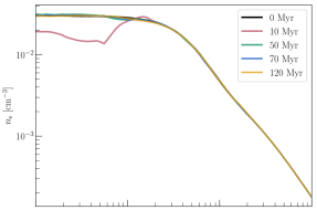
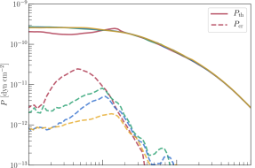
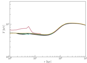
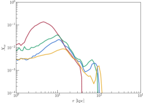
Figure 1: Radial profiles of the gas for the initial conditions at $0\ \mathrm{Myr}$ (black) and the fiducial model at stated times. The number density $n_{e}$ is volume-weighted, the temperature $T$ is mass-weighted and the CR pressure $P_{\mathrm{cr}}$ as well as the thermal pressure $P_{\mathrm{th}}$ are both volume-weighted. The CR-to-thermal pressure ratio $X_{\mathrm{cr}}$ is obtained by dividing both volume-weighted quantities. The propagating jet is visible as a low-density and hot feature close to the cluster centre at 10 Myr. The CRs are distributed within the inner $100\ \mathrm{kpc}$ and their profile drops off steeply at larger radii.

2 Methods and simulation models

Here, we introduce our numerical set-up of the cluster model and the adopted magnetic structure of the ICM. We employ magneto-hydrodynamical (MHD) simulations with the moving-mesh code arepo (Springel, 2010) that evolves thermodynamic quantities of the gas on an unstructured moving mesh defined by the Voronoi tessellation of a set of discrete points that initially obey a quasi-Lagrangian distribution. Of particular importance for this work are our models for launching AGN jets and CR transport, which we describe in detail here. An overview of our simulation models closes this section.

2.1 Initial conditions

By analogy with Weinberger et al. (2017), we model the cluster density distribution with a Navarro-Frenk-White (NFW) profile (Navarro et al., 1996, 1997) with virial radius $R_{200,\mathrm{c}}=2.12\ \mathrm{Mpc}$, virial mass $M_{200,\mathrm{c}}=10^{15}\ \mathrm{M}_{\odot}$, and concentration parameter $c_{\mathrm{NFW}}=5$. The electron number density $n_{\mathrm{e}}$ is modelled after the Perseus galaxy cluster and based on a double-beta profile fit to the de-projected density distribution from X-ray observations (Churazov et al., 2003). In addition, the number density is scaled in order to retain a gas fraction of $16\%$ within $R_{200,\mathrm{c}}$:

$$\begin{split}n_{\mathrm{e}}&=26.9\times 10^{-3}\left[1+\left(\frac{r}{57\ \text{kpc}}\right)^{2}\right]^{-1.8}\text{cm}^{-3}\\ &\quad+2.8\times 10^{-3}\left[1+\left(\frac{r}{200\ \text{kpc}}\right)^{2}\right]^{-0.87}\text{cm}^{-3}.\end{split}$$ (1)

The pressure in each cell is obtained from the assumption of hydrostatic equilibrium and the restriction that the pressure vanishes at a radius of $3\ \mathrm{Mpc}$. Initially, we adopt a Cartesian mesh with a box size of $1.5\ \mathrm{Mpc}$ that we iteratively refine to ensure similar mass content per cell. This yields an adaptive mesh with smoothly increasing cell sizes towards larger radii.

Gravity is treated as a static background provided by a NFW dark matter distribution, neglecting the effects of self-gravity and the gravitational interactions with the SMBH. We show radial profiles of the initial conditions of the electron number density $n_{\mathrm{e}}$, temperature $T$, and thermal pressure $P_{\mathrm{th}}$ in Fig. 1 (note that there are no CRs in the initial conditions).

To mimic a realistic ICM, we generate a Gaussian-distributed, turbulent magnetic field B (see Appendix A, for details). First, we lay down our initial magnetic field on a Cartesian mesh, which needs to have a resolution that is smaller than the smallest (Lagrangian) cell size of our high-resolution initial conditions, $\Delta x=700\ \mathrm{pc}$. Fourier transforming such a large Cartesian grid is numerically not feasible. Thus, for our high-resolution simulation we set up three nested meshes, with resolutions decreasing from the cluster centre. Generally, the magnetic field meets the following requirements:

1. B is divergence-free: $\bm{\nabla}\mathchoice{\mskip 3.0mu\lower 0.86108pt\hbox{\scalebox{1.5}{$\cdot$}}\mskip 3.0mu}{\mskip 3.0mu\lower 0.86108pt\hbox{\scalebox{1.5}{$\cdot$}}\mskip 3.0mu}{\lower 1.29167pt\hbox{\scalebox{1.2}{$\cdot$}}}{\lower 1.29167pt\hbox{\scalebox{1.2}{$\cdot$}}}\textbf{{B}}=0$;

2. B follows a Kolmogorov spectrum in the inertial range for wave numbers larger than the injection scale $k_{\mathrm{inj}}$, and a random white noise power spectrum for $k<k_{\mathrm{inj}}$;

3. $\textbf{{B}}^{2}$ is scaled at each radius to obtain a constant average magnetic-to-thermal pressure ratio of $X_{B,\mathrm{ICM}}$;

4. B fields on different nested meshes do not interconnect.

The resulting cluster magnetic field is then interpolated from this nested mesh onto our adaptive, smoothly varying mesh. To ensure pressure equilibrium in the initial conditions, we adopt temperature fluctuations of the form $nk_{\mathrm{B}}\delta T=-\delta\textbf{{B}}^{2}/(8\pi)$. We then relax our mesh to obtain a computationally more efficient non-degenerate tessellation structure for arepo. However, this setup does not balance the magnetic tension. The resulting turbulent motions initiate the decay of magnetic power. To reinitialize the prescribed magnetic-to-thermal pressure ratio, we rescale the temperature as well as the magnetic field to the desired initial magnetic-to-thermal pressure ratio $X_{B,\mathrm{ICM}}$ while maintaining hydrostatic equilibrium.

The described procedure generates our initial conditions for simulations with a turbulent magnetic field. The initiated turbulence during the relaxation of the mesh initiates bulk velocities, which remain part of the initial conditions. For our comparison simulations without a magnetic field, we proceed as before, but set $\textbf{{B}}={\bf 0}$. Thus, the atmosphere remains turbulent through the presence of initial flows and pressure irregularities. However, these runs show a lower degree of turbulence than the runs with finite magnetic field as the magnetic tension can drive and sustain turbulence on longer time scales.

As explained above, the stresses of the tangled magnetic field induce turbulent gas motions. In the absence of a driver of turbulence (as in our simulations) the turbulence gradually dissipates and the magnetic field strength and gas velocities decrease as a function of time.

2.2 Jet model

To study the influence of a SMBH-driven and CR-filled jet in a turbulent cluster environment, we employ the jet model of Weinberger et al. (2017). Here, we provide a brief summary of the implementation and describe modifications related to CR acceleration, CR cooling and the magnetic isolation of the injection region.

The jet becomes active at time $t$ after the last injection event at $t_{\mathrm{inj}}$ when the available energy to the jet, $\dot{E}_{\mathrm{jet}}(t-t_{\mathrm{inj}})$, exceeds the required energy to redistribute the gas considering adiabatic changes and inject a predefined amount of energy (thermal and non-thermal). When the jet is active, the model identifies two opposing jet regions close to the black hole. A low density state ($\rho_{\mathrm{jet}}/\rho_{\mathrm{ICM}}\sim 10^{-4}$) is set up in pressure equilibrium with the surrounding medium. Mass and thermal energy are redistributed to and from neighbouring cells to ensure mass conservation. If desired, a magnetic field is included in a purely toroidal configuration. Due to gas flows in the bubble, the magnetic field is reshaped, but maintains its helical morphology. After accounting for adiabatic losses, the remaining jet energy is injected as kinetic energy to launch a bipolar outflow. To identify the bubble, an advective scalar $X_{\mathrm{jet}}$ is used, which corresponds to the mass fraction of the jet material in the cell. In the remainder of this work we refer to $X_{\mathrm{jet}}$ as jet tracer. The tracer is initialised in the jet injection region with a value of $X_{\mathrm{jet}}=1$. The strong density contrast between bubble and cluster is maintained through refinement criteria based on the density gradient and cell volume (for details, see Weinberger et al., 2017). Throughout this work, we define lobe material to exhibit a jet mass fraction $X_{\mathrm{jet}}>10^{-3}$ and checked that the conclusions of this paper are invariant with respect to variations of this choice.

The discrepancy between the inferred pressure of observed bubbles (via minimum energy arguments of radio observations) and the ambient ICM pressure (as inferred from X-ray observations) argues for a significant pressure contribution of CR protons that cannot directly be inferred by any interaction process due to the very low bubble densities (Bîrzan et al., 2008; Croston et al., 2008; Laing & Bridle, 2014; Croston & Hardcastle, 2014; Heesen et al., 2018). CRs could be accelerated at internal shocks of jets (Perucho & Martí, 2007). The strong non-thermal emission in knots observed in jets supports this mechanism (Worrall, 2009; Laing & Bridle, 2013; Duran et al., 2016). As we do not resolve internal shocks explicitly, we treat CR injection in a subgrid model. As most of the injected kinetic energy would immediately be thermalized, we instead ensure a minimum CR-to-thermal energy fraction $X_{\mathrm{cr,acc}}=E_{\mathrm{cr}}/E_{\mathrm{th}}=1$ in every computational cell inside the jet/lobe for a time $\tau_{\mathrm{acc}}=2\tau_{\mathrm{jet}}$, where $\tau_{\mathrm{jet}}$ is the jet lifetime. When varying $\tau_{\mathrm{acc}}$ we find that the resulting dynamical effects of late-time accelerated CRs ($t>\tau_{\mathrm{jet}}$) are negligible. This is an important difference in comparison to Weinberger et al. (2017) where the bubble CR pressure is specified at jet launch and successive CR acceleration in the jet is not accounted for, which yields a sub-dominant CR population.

2.3 CR transport

CRs as charged particles are bound to stay on flux-frozen magnetic field lines. As the magnetic field is transported alongside the gas, so are CRs. In addition to advection, CRs scatter on magnetic fluctuations which leads to transport by diffusion and streaming relative to the rest frame of the gas, mainly along the direction of the local mean magnetic field, which coincides with the large-scale field (Pfrommer et al., 2017).

Anisotropically moving CRs in the frame of propagating Alfvén waves are unstable to the streaming instability (Kulsrud & Pearce, 1969). These CRs resonantly excite Alfvén waves, which in turn causes the CRs’ pitch angles to scatter and eventually to isotropize in the Alfvén frame (that moves with speed $v_{\mathrm{A}}$). Hence, in galaxy clusters, the streaming velocity $v_{\mathrm{s}}$ relative to the thermal plasma corresponds approximately to the Alfvén velocity, i.e., $v_{\mathrm{s}}-v_{\mathrm{A}}\sim{}c^{2}/(3\nu{}l_{\mathrm{cr}})$, where $\nu$ is the pitch angle scattering rate and $l_{\mathrm{cr}}=P_{\mathrm{cr}}/\nabla P_{\mathrm{cr}}$ is the CR gradient length scale (Kulsrud, 2005). In addition, CRs diffuse along field lines with a diffusion coefficient $\tilde{\kappa}\equiv{}c^{2}/(3\nu)\sim(v_{\mathrm{s}}-v_{\mathrm{A}})l_{\mathrm{cr}}$, which makes diffusion negligible compared to streaming in the strong scattering limit. Consequently, we introduce an effective CR diffusion coefficient $\kappa_{\mathrm{cr,A}}\sim{}l_{\mathrm{cr}}v_{\mathrm{A}}$ that emulates the combined effects of streaming and spatial diffusion (Sharma et al., 2009; Wiener et al., 2017).

Different damping mechanisms dissipate Alfvén waves, causing the streaming CRs in steady state to continuously transfer part of their energy into heat via Alfvén wave heating with a rate

$$\mathcal{H}_{\mathrm{cr}}=\left|\bm{v}_{\mathrm{A}}\mathchoice{\mskip 3.0mu\lower 0.86108pt\hbox{\scalebox{1.5}{$\cdot$}}\mskip 3.0mu}{\mskip 3.0mu\lower 0.86108pt\hbox{\scalebox{1.5}{$\cdot$}}\mskip 3.0mu}{\lower 1.29167pt\hbox{\scalebox{1.2}{$\cdot$}}}{\lower 1.29167pt\hbox{\scalebox{1.2}{$\cdot$}}}\bm{\nabla}{P}_{\mathrm{cr}}\right|.$$ (2)

Note the dependence of the Alfvén heating rate on the CR pressure gradient. This directly relates $\mathcal{H}_{\mathrm{cr}}$ to the CR diffusion coefficient $\kappa_{\mathrm{cr,A}}$ in our effective model.

Following this self-confined picture, CRs are treated as a secondary fluid with adiabatic index $\gamma_{\text{cr}}=4/3$ (Pfrommer et al., 2017). We emulate streaming through a combination of anisotropic diffusion and Alfvén losses (Wiener et al., 2017). Our CRs are advected with the gas and anisotropically diffuse with a constant diffusion coefficient $\kappa_{\parallel}=10^{29}\ \mathrm{cm}^{2}\mathrm{s}^{-1}$ along B and $\kappa_{\perp}=0$ perpendicular to it (Pakmor et al., 2016b). The particular value of $\kappa_{\parallel}$ has been choosen so that it produces self-consistent results in our simulations (as we will see later in Section 5.1).

The CR distribution in the lobes quickly becomes uniform as the magnetic field confines the CRs initially to stay within the lobes. This leads to a negligible CR pressure gradient and hence an insignificant Alfvén wave cooling rate inside lobes. In our simulations, insufficiently resolved steep gradients at the lobe interface would lead to artificially large (numerical) cooling rates. We prevent this by imposing a maximum jet tracer threshold $X_{\mathrm{jet,cool}}\leq 10^{-3}$ for Alfvén wave cooling to be active (for a discussion, see Appendix C). Our simulations also include the cooling of CRs through Coulomb and hadronic interactions (Pfrommer et al., 2017), which are however much smaller here in comparison to Alfvénic losses.

Physically, the jet fluid is magnetically unconnected to the ICM. In order to study the evolution of the diffusing CR distribution accurately, the jet launching region needs to be magnetically isolated to prevent spurious diffusion at the resolution limit along field lines that connect the jet launch region to the exterior ICM. Many individual injection events are present in our simulation, which require accurate magnetic isolation before each individual event. To this end, we project out the radial magnetic field components:

$$\textbf{{B}}\to\left[1-g(r)\hat{\textbf{{r}}}\hat{\textbf{{r}}}\right]\textbf{{B}},$$ (3)

where $\hat{\textbf{{r}}}$ is the radial unit vector measured from the centre of our spherical jet launching region and $g(r)=1-\left|\cos\left(0.5\pi\left(x+\Delta x-1\right)/{\Delta x}\right)\right|$ for $1-\Delta x<x<1+\Delta x$, where $x=r/r_{\textrm{jet}}$, $\Delta x=0.25$, and $r_{\mathrm{jet}}$ is the radius of the jet launching region. Jets are launched from two regions on opposite sides of the centre. During the first injection event of a jet, the two bimodal jet regions are isotropically isolated, i.e., across the entire spherical surface (see equation 3). At all subsequent injection events while the jet is active, only the bubble hemisphere closer to the SMBH is isolated in order to retain the velocity structure in the direction of motion of the jet.

2.4 Simulation models

$P_{\text{jet}}$	$X_{{B},\mathrm{ICM}}$	$X_{{B},\mathrm{jet}}$	$\tau_{\text{jet}}$	$\kappa_{\parallel}$	$E_{\mathrm{jet}}$
$[\text{erg}\,\text{s}^{-1}]$			$[\text{Myr}]$	$[\text{cm}^{2}\,\text{s}^{-1}]$	$[10^{59}\,\mathrm{erg}]$
simulations with CRs
$4\times 10^{43}$	$0.05$	$0.1$	10	$10^{29}$	$~{}~{}0.13$
$4\times 10^{43}$	$0.05$	$0.1$	25	$10^{29}$	$~{}~{}0.31$
$4\times 10^{43}$	$0.05$	$0.1$	50	$10^{29}$	$~{}~{}0.63$
$1\times 10^{44}$	$0.05$	$0.1$	10	$10^{29}$	$~{}~{}0.32$
$1\times 10^{44}$	$0.05$	$0.1$	25	$10^{29}$	$~{}~{}0.79$
$1\times 10^{44}$	$0.05$	$0.1$	50	$10^{29}$	$~{}~{}1.58$
$2\times 10^{44}$	$0.05$	$0.1$	10	$10^{29}$	$~{}~{}0.63$
${\bf 2\times 10^{44}}$	${\bf 0.05}$	${\bf 0.1}$	25	${\bf 10^{29}}$	${\bf~{}~{}1.58}$
$2\times 10^{44}$	$0.05$	$0.1$	50	$10^{29}$	$~{}~{}3.15$
$4\times 10^{44}$	$0.05$	$0.1$	10	$10^{29}$	$~{}~{}1.26$
$4\times 10^{44}$	$0.05$	$0.1$	25	$10^{29}$	$~{}~{}3.15$
$4\times 10^{44}$	$0.05$	$0.1$	50	$10^{29}$	$~{}~{}6.31$
$1\times 10^{45}$	$0.05$	$0.1$	10	$10^{29}$	$~{}~{}3.15$
$1\times 10^{45}$	$0.05$	$0.1$	25	$10^{29}$	$~{}~{}7.88$
$1\times 10^{45}$	$0.05$	$0.1$	50	$10^{29}$	$15.77$
simulations without CRs
$2\times 10^{44}$	$0.05$	$0.1$	25	$0$	$~{}~{}1.58$
$2\times 10^{44}$	$0~{}~{}~{}~{}$	$0.1$	25	$0$	$~{}~{}1.58$
$2\times 10^{44}$	$0.05$	$0~{}~{}$	25	$0$	$~{}~{}1.58$
$2\times 10^{44}$	$0~{}~{}~{}~{}$	$0~{}~{}$	25	$0$	$~{}~{}1.58$

Table 1: Jet parameters of the different models with combined jet power $P_{\text{jet}}$ of the bipolar outflow, external magnetic-to-thermal pressure ratio $X_{{B},\mathrm{ICM}}$, jet magnetic-to-thermal pressure ratio $X_{{B},\text{jet}}$, time of activity of the jet $\tau_{\mathrm{jet}}$, CR diffusion coefficient along the magnetic field $\kappa_{\parallel}$ and jet energy $E_{\mathrm{jet}}=P_{\mathrm{jet}}\tau_{\mathrm{jet}}$. The lower part of the table corresponds to our control runs without CRs, which are used for the analysis of the bubble stability. The fiducial run is marked in boldface.

Our MHD simulations are performed with the moving-mesh code arepo (Springel, 2010), using an improved second-order hydrodynamic scheme with least-squares-fit gradient estimates and a Runge-Kutta time integration (Pakmor et al., 2016a). The MHD fluxes across cell interfaces are computed with an HLLD Riemann solver (Pakmor et al., 2011; Pakmor & Springel, 2013) adopting the Powell scheme for divergence control (Powell et al., 1999).

The bubble evolution is studied in a set of simulations listed in Table 1. The jets are active for a prescribed time $\tau_{\mathrm{jet}}$ with a certain jet power $P_{\mathrm{jet}}$. Our fiducial model corresponds to $P_{\mathrm{jet}}=2~{}\times~{}10^{44}\ \mathrm{erg}\ \mathrm{s}^{-1}$, $\tau_{\mathrm{jet}}=25\ \mathrm{Myr}$, $X_{B,\mathrm{ICM}}=0.05$, $X_{B,\mathrm{jet}}=0.1$ and $\kappa_{\parallel}=10^{29}\ \mathrm{cm}^{2}\ \mathrm{s}^{-1}$. We use this model in the analysis unless stated otherwise.

Jet parameters
Jet density	$\rho_{\text{target}}$	$10^{-28}\ \text{g}\ \text{cm}^{-3}$
Jet launching region	$r_{\mathrm{j}}$	$5\ \text{kpc}$
CR acceleration	$X_{\text{cr,acc}}$	$1$
Magnetic field parameters
Injection scale	$k_{\text{inj}}$	$37.5^{-1}\ \text{kpc}^{-1}$
Resolution
Target mass	$m_{\text{target},0}$	lower res.: $1.5\times 10^{6}\ \text{M}_{\odot}$
		high res.: $1.5\times 10^{5}\ \text{M}_{\odot}$
Target volume	$V_{\text{target}}^{1/3}$	lower res.: $405\ \text{pc}$
		high res.: $188\ \text{pc}$
Minimum volume	$V_{\text{min}}$	$V_{\text{target}}/2$

Table 2: A summary of our adopted parameters of the simulation.

Sub-grid parameters and those responsible for the resolution of our simulation are given in Table 2. In Weinberger et al. (2017), we showed that the distance travelled by bubbles depends on the numerical resolution of the jet. Here, we focus on the previously dubbed high-resolution simulation. The numerical convergence of our results in comparison to lower resolution simulations is discussed in Appendix B. When we compare several simulation models with varying parameters, we use the lower resolution simulations as this recovers qualitatively the same evolution of the jet at a significantly lower computational cost.

If included in the lobes ($X_{\mathrm{jet}}>10^{-3}$), CRs are generally accelerated for time $\tau_{\mathrm{acc}}=2\tau_{\mathrm{jet}}$ and we use a conversion fraction from thermal-to-CR energy of $X_{\mathrm{cr,acc}}=1$. Reducing the fraction $X_{\mathrm{cr,acc}}$ only changes the normalisation of our CRs but has no significant impact on the studied features. Also, a much larger fraction of CRs is disfavoured as FRI jets are slowed down through the entrainment of ambient material. A remaining population of shocks seems unlikely to accelerate significant portions of the entrained protons. The conclusions of this paper also remain robust against variations of $\tau_{\mathrm{acc}}$ as long as $\tau_{\mathrm{acc}}\geq\tau_{\mathrm{jet}}$.

While magnetic tension initially generate significant levels of turbulence, this decays over the run time of our simulation since we do not model large scale flows due to substructure (Bourne & Sijacki, 2017) and neglect gas cooling, which also induces motions. In reality, the cooling gas accretes onto the central SMBH, powering jets in this process, leading to highly variable jet powers and lifetimes. Here, we instead decided to impose predefined jet energies to gain insight into the parametric dependencies of mixing, morphologies and CR distributions more easily. We postpone modelling of self-consistent jet injection through accreted cooling gas, which will enable us to study the long-term stability of the CC cluster due to CR heating.

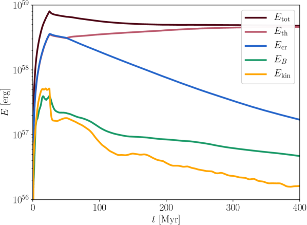
Figure 2: The time evolution of the energy components of the lobe. The lobe is defined as cells with jet mass fraction $X_{\mathrm{jet}}>10^{-3}$. The thermal and CR energy are initially in equipartition. Later, CRs diffuse out of the lobe and thermal gas is entrained, which leads to an overall increase in thermal energy after the jet becomes inactive.

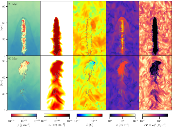
Figure 3: The mass density $\rho$, CR energy density $\epsilon_{\mathrm{cr}}$, magnetic field strength $B$, velocity $v$ and vorticity squared $(\nabla\times v)^{2}$ of the fiducial run are portrayed at times $20$ Myr and $60$ Myr. The images correspond to projections of thin layers ($100\ \mathrm{kpc}\times 60\ \mathrm{kpc}\times 4\ \mathrm{kpc}$) centred at $(50,0,0)$ and weighted by cell volume except for the velocity, which is weighted by the density. The grey contour corresponds to the jet tracer value $X_{\mathrm{jet}}=10^{-3}$. The characteristic transition from jet to lobe becomes evident.

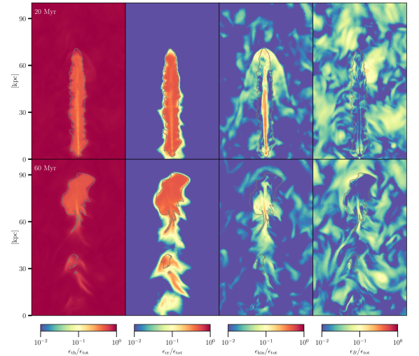
Figure 4: The thermal $\epsilon_{\mathrm{th}}$, CR $\epsilon_{\mathrm{cr}}$, kinetic $\epsilon_{\mathrm{kin}}$ and magnetic $\epsilon_{B}$ energy density, which are normalised to the total energy density $\epsilon_{\mathrm{tot}}=\epsilon_{\mathrm{th}}+\epsilon_{\mathrm{cr}}+\epsilon_{\mathrm{kin}}+\epsilon_{B}$ of the fiducial run, are portrayed at times $20$ Myr and $60$ Myr. The images correspond to projections of thin layers ($100\ \mathrm{kpc}\times 60\ \mathrm{kpc}\times 4\ \mathrm{kpc}$), which are volume weighted and centred at $(50,0,0)$. The grey contour corresponds to the jet tracer value $X_{\mathrm{jet}}=10^{-3}$.

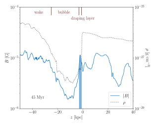
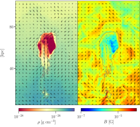
Figure 5: On the left, we show the mean magnetic field strength (blue) along a thin radially-aligned cylinder ($r=1\ \mathrm{kpc}$) through the bubble as a function of distance $z$ to the stagnation point at 45 Myr. We mark the thin magnetic draping layer with a filled blue contour and locate the extent of the bubble and its wake. To identify the extent of the bubble, the density is overlaid (black dashed). On the right, we show the density and magnetic field strength. The arrows correspond to the kinetic energy flux and the magnetic field directions, respectively, and the arrow length encodes the magnitude of these variables. The images correspond to projections of thin layers ($100\ \mathrm{kpc}\times 60\ \mathrm{kpc}\times 4\ \mathrm{kpc}$) centred on the wake of the bubble. The grey contour corresponds to the jet tracer value $X_{\mathrm{jet}}=10^{-3}$. It becomes apparent that the magnetic field amplification at the bubble surface is not due to the compression of gas but rather due to draping in the direction of movement. The width of the draping layer corresponds to the theoretically predicted value of $\approx 2\ \mathrm{kpc}$.

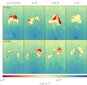
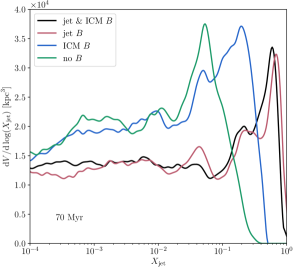
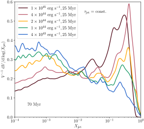
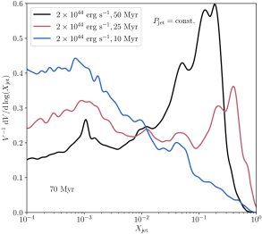
Figure 6: The mixing efficiency of the bubble for different magnetic field parameters of our lower resolution simulations. On the top left, we show lobe-centred projections of thin layers ($80\ \mathrm{kpc}\times 50\ \mathrm{kpc}\times 4\ \mathrm{kpc}$) of the density with jet mass fractions overlaid ($X_{\mathrm{jet}}=10^{-3}$) for four simulations without CRs indicated above the panels. On the top right, the volume covered by gas, $\mathrm{d}V/\mathrm{d}\log(X_{\mathrm{jet}})$, with a given jet mass fraction $X_{\mathrm{jet}}$ is shown at 70 Myr for the same four simulations. The presence of magnetic fields significantly suppresses mixing in the bubble. The bottom panels portray the normalised volume covering fraction of a given jet mass fraction, $V^{-1}\ \mathrm{d}V/\mathrm{d}\log(X_{\mathrm{jet}})$. On the bottom left, we vary the jet power at constant time of jet activity $\tau_{\mathrm{jet}}=25\ \mathrm{Myr}$. On the bottom right, we show bubbles inflated by jets of constant power $P_{\mathrm{jet}}=2\times 10^{44}\ \mathrm{erg/s}$. The peak of the volume fraction moves to the left for less energetic jets (decreased $P_{\mathrm{jet}}$ or $\tau_{\mathrm{jet}}$) indicating increased mixing efficiencies for these jets. The lines are smoothed for clarity.

3 Jet and bubble evolution

First, we discuss the evolution of our jets and bubbles in terms of global quantities and with detailed maps of thermodynamical quantities.

3.1 Global evolution

The jets are initialised with a dominant kinetic energy component. Through dissipation much of this kinetic energy is quickly thermalized. This would lead to thermally dominated lobes, in conflict with X-ray observations. The subgrid acceleration scheme employed for CR maintains them in equipartition with thermal energy until $2\tau_{\mathrm{acc}}$. Thus, CRs share a significant fraction of the energy and pressure in these simulations as shown in Fig. 2 which shows the time evolution of different energy components in the lobes. The strong dissipation of the kinetic energy of the jets effectively transfers kinetic energy into CR and thermal energy. Compared to the initial magnetic-to-thermal pressure ratio in the jet $X_{B,\mathrm{jet}}=0.1$, the ratio drops by more than an order of magnitude due to the strong increase of thermal energy.

The thermal energy increases at later times whereas the CR energy decreases in Fig. 2. We adopt a morphology-based definition of lobes with a jet mass fraction exceeding $10^{-3}$, which includes by definition heavily mixed cells. Thereby, mixing leads to an increase of mass and thermal energy in the lobes at later times. On the other hand, CRs continuously diffuse out of the bubbles, lowering their total energy. Note that CR energy losses due to cooling in the bubbles is solely restricted to the (almost negligible) hadronic and Coulomb losses as we suppress Alfvénic cooling in the bubble region (see Section 2.3).

The evolution of the thermodynamic cluster profiles (Fig. 1) shows a decrease in density and an increase in temperature at early times, which corresponds to the high thermal energy of the propagating jet. Because this hot gas has such a low-density it remains invisible in X-ray maps, which is in agreement with observations (e.g., Leccardi & Molendi, 2008). After the jet terminates and the bubbles rise buoyantly, the mean thermodynamic profiles nearly recover the initial conditions.

3.2 Morphology

The jet driving phase and subsequent phase of buoyant rise of the bubble are portrayed in Figs. 3 and 4 at 20 Myr and 60 Myr for the fiducial run. Figure 3 shows various thermodynamic variables projected in thin slices and Fig. 4 displays various energy densities, normalised to the total energy density. This enables direct comparisons of the dynamical impact of the different components.

Initially, the jet penetrates into the ambient medium forming a bow shock at its tip. The shock is visible in the first row of Fig. 3 as a discontinuity with increased density and velocity. The continuous mass flux is deflected at the tangential discontinuity between the jet and shock. The strong inflow expands horizontally and mixes with the shocked ICM gas streaming around the jet. This leads to the creation of an extended, highly turbulent region with high vorticity, see Fig. 3.

After the jet is switched off at 25 Myr, the remaining directed kinetic energy flux thermalises and catches up with the previously injected material forming a bubble, whose evolution is now solely driven by buoyancy. The high contrast in density between the lobes and the ambient medium makes the setup susceptible to the Rayleigh-Taylor instability. Thus, strong inflows develop in the wake of the bubble. In the second row of Fig. 3, the developing strong vorticity and high velocities are visible in the wake. They cause strong mixing of the bubble material with the ambient medium, which is accompanied by an increase in density.

The low magnetic field strength renders it dynamically irrelevant in the bulk of the ICM (Fig. 4). However, there are two cases where the dynamics amplifies the magnetic field to the point that it plays a significant role for the evolution of the system: first, there is significant magnetic field amplification in the wake of the bubble (Figs. 3 and 4). This is due to bubble-scale eddies that converge in the wake and adiabatically compress the field and stretch it by the strong shear flows that become evident in the vorticity map.

Second, the upwards motion of the bubbles in the ICM causes magnetic field lines of the IGM to accumulate at the leading surface of the rising bubble, which is a tangential discontinuity (Pfrommer & Dursi, 2010). These draped magnetic field lines lead to the suppression of Kelvin-Helmholtz and Rayleigh-Taylor instabilities (see also Section 4.1, for a detailed discussion). The bubble is eventually disrupted by strong uplifts of wake material, which are able to penetrate through the centre of the bubble. If turbulence is absent the resulting torus structure remains stable on timescales of $>100\ \mathrm{Myr}$ (Weinberger et al., 2017). In our simulations, the onset of a developing (deformed) toroidal structure is visible after $\sim 70-100\ \mathrm{Myr}$ (see Fig. 6). However, the turbulent asymmetrical flow pattern of the uplift causes the break up of the lobe into two main pieces. If enough low density material remains, the two cavities can continue to rise as two independent bubbles until the uplift becomes too strong again and causes them to also break apart.

In addition to advection, CRs are allowed to anisotropically diffuse along magnetic field lines. However, the draped magnetic layer on top of the bubble confines the CRs inside and prevents escape ahead of the bubble. Instead, CRs are able to diffuse out of the lower part of the bubble along the strongly amplified magnetic filaments, which are bent by the strong uplift and align with the jet axis (see Fig. 3). The jet evolution and subsequent creation of the bubble is in excellent agreement with previous work (e.g., Lind et al., 1989; Reynolds et al., 2002), suggesting that the addition of internal and external magnetic fields as well as CRs does not change the overall evolution of the system.

4 Magnetic field evolution

In this section, we study the effect of magnetic draping at the bubble interface, amplification of magnetic fields in the bubble’s wake, and the effect of magnetic fields on the mixing efficiency of the bubble fluid with the ICM.

4.1 Magnetic draping and amplification

Objects moving at super-Alfvénic speed through a magnetised medium accumulate magnetic field lines at their interface. This magnetic draping effect occurs only if the magnetic coherence scale is sufficiently large, i.e., $\lambda_{B}\gtrsim R/\mathcal{M}_{\mathrm{A}}$ where $R$ is the curvature radius at the stagnation point and $\mathcal{M}_{\mathrm{A}}$ is the Alfvénic Mach number (Pfrommer & Dursi, 2010). In a steady state, the rate at which new magnetic field lines enter this strongly magnetised sheath balances the rate at which magnetic field lines are advected over the bubble’s surface to eventually leave the draping layer. The magnetic tension exerted by this draping layer slows down the object as the magnetic field is anchored in the ICM in ideal MHD and thus acquires a large inertia (Dursi & Pfrommer, 2008). Moreover, draping makes the object more resilient against interface instabilities of the Kelvin-Helmholtz or Rayleigh-Taylor type (Dursi, 2007). This draping layer inhibits any particle transport across the bubble surface such as CR diffusion (Ruszkowski et al., 2008), heat conduction by thermal electrons and momentum transport or viscosity by thermal protons, which stabilises sharp temperature and density transitions observed in the ICM (i.e., cold fronts) against disruption (Vikhlinin et al., 2001; Lyutikov, 2006; Asai et al., 2007). Previous simulations acknowledge the stabilising effect of magnetic fields (Jones & De Young, 2005; O’Neill et al., 2009; Bambic et al., 2018). Here, for the first time, we present results for the case of self-consistently inflated bubbles in a realistic turbulent magnetised environment.

Magnetic draping creates a layer of thickness $l$ that is smaller than the curvature radius $R$ of the bubble at the stagnation point by (Dursi & Pfrommer, 2008):

$$\frac{l}{R}=\frac{1}{6\alpha\mathcal{M}^{2}_{\mathrm{A}}}=\frac{1}{3\alpha\beta\gamma\mathcal{M}^{2}}=\frac{1}{3}\frac{B_{\mathrm{ICM}}^{2}}{B_{\mathrm{max}}^{2}},$$ (4)

where $\alpha$ describes the magnetic-to-ram pressure ratio at the stagnation point ($B_{\mathrm{max}}^{2}/8\pi=\alpha\rho v^{2}$), $\mathcal{M}_{\mathrm{A}}$ corresponds to the Alfvénic Mach number $\mathcal{M}_{\mathrm{A}}=v/v_{\mathrm{A}}$, $\mathcal{M}$ is the sonic Mach number, $\gamma=5/3$ is the adiabatic index and $X_{B,\mathrm{ICM}}=\beta^{-1}$ is the thermal-to-magnetic pressure ratio in the upstream ICM. In our simulations, $X_{B,\mathrm{ICM}}=0.05$, we determine $\mathcal{M}\approx 0.2$ and take $\alpha\approx 2$ from Dursi & Pfrommer (2008). Thus, we expect draping layer thickness $l\approx 2\ \mathrm{kpc}$ for a curvature radius $R=20\ \mathrm{kpc}$ at our simulated bubble. This implies that we are able to numerically resolve the draping layer due to our refinement prescriptions.

Figure 5 (left-hand panel) shows the magnetic field strength (blue line) along the stagnation line of the bubble. At the bubble edge, which is clearly identified by the sharp increase in density (black dashed), the magnetic field shows a pronounced narrow peak with width $l\approx 2\ \mathrm{kpc}$. In agreement with our theoretical predictions, the magnetic field rises from its mean value of $B_{\mathrm{ICM}}\approx 5~{}\mu$G to $B_{\mathrm{max}}\approx 10~{}\mu$G in the draping layer (see equation 4). In the magnetic field map (right-hand panel in Fig. 5), a thin enhanced magnetic field layer is also visible that corresponds to the draping layer surrounding the bubble. Consequently, we confirm that magnetic draping is an active process in bubble dynamics in agreement with previous studies (Ruszkowski et al., 2007; Dursi & Pfrommer, 2008).

In the wake of the jet, magnetic field lines are stretched by differential motions and compressed by converging downdrafts that compensate the upwards motion of the bubble. This process amplifies magnetic fields in the wake and aligns field lines with the jet axis (Fig. 5), in agreement with previous findings (O’Neill & Jones, 2010; Mendygral et al., 2012). This has important consequences for the CRs, which are confined in the bubble by the draped magnetic field at the leading interface. Hence, escape from the bubble only becomes possible in its wake as the converging eddies connect the bubble interior magnetically with the ICM via the amplified magnetic filaments (see Figs. 3 and 5). As a result, CRs are conducted diffusively along the magnetic filaments towards the cluster centre in the opposite direction to the CR pressure gradient (Fig. 3).

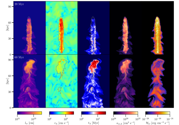
Figure 7: Quantities related to CR transport in jet and lobe. We show the CR gradient length scale $l_{\mathrm{cr}}=P_{\mathrm{cr}}/\bm{\nabla}{}P_{\mathrm{cr}}$, the Alfvén velocity $v_{\mathrm{A}}$, the Alfvén cooling time scale of CRs, $t_{\mathrm{A}}=l_{\mathrm{cr}}/v_{\mathrm{A}}$, the instantaneous CR diffusion coefficient $\kappa_{\mathrm{cr,A}}=v_{\mathrm{A}}l_{\mathrm{cr}}$ and the Alfvén heating rate $\mathcal{H}_{\mathrm{cr}}=\left|\bm{v}_{\mathrm{A}}\cdot\bm{\nabla}{P}_{\mathrm{cr}}\right|$ of the fiducial run at $20$ Myr and $60$ Myr. Here, we also display the measured heating rate inside the lobes to illustrate the strong increase of Alfvén heating at the lobe edges due to the large numerical CR pressure gradients there, which is for this reason suppressed in our simulations. The images correspond to projections of thin layers ($100\ \mathrm{kpc}\times 60\ \mathrm{kpc}\times 4\ \mathrm{kpc}$) weighted with the volume and centred at $(50,0,0)$. We only show $l_{\mathrm{cr}}$, $t_{\mathrm{A}}$, $\kappa_{\mathrm{cr,A}}$ and $\mathcal{H}_{\mathrm{cr}}$ in regions with $\epsilon_{\mathrm{cr}}>10^{-14}\ \mathrm{erg}\ \mathrm{cm}^{-3}$ to exclude an energetically subdominant CR population, which has partially experienced numerical diffusion. The CR gradient is unavailable due to numerical reasons for individual saturated cells which are shown with yellow. The grey contour corresponds to the jet tracer value $X_{\mathrm{jet}}=10^{-3}$.

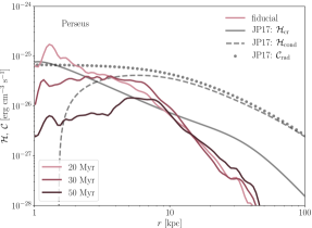
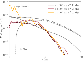
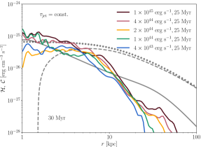
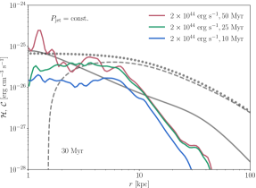
Figure 8: Radial profiles of the Alfvén heating rate in the ICM due to CR streaming, $\mathcal{H}_{\mathrm{cr}}$ (restricting ourselves to ICM simulation cells with $X_{\mathrm{jet}}<10^{-3}$ and using our lower resolution simulations). We compare our simulation to a spherically symmetric, steady state solution in which CR heating (solid) and conductive heating ($\mathcal{H}_{\mathrm{cond}}$, dashed) balances radiative cooling ($\mathcal{C}_{\mathrm{rad}}$, dotted) in the Perseus cluster (Jacob & Pfrommer, 2017a). On the upper left, we show different radial profiles at times 20, 30 and 50 Myr for our fiducial model. On the upper right, we compare profiles of jets with similar energy ($E_{\mathrm{jet}}\approx 1.58\times 10^{59}\ \mathrm{erg}$) but different $P_{\mathrm{jet}}$ and $\tau_{\mathrm{jet}}$: the heating rate profile is steeper for low-luminosity jets with longer activity times. On the bottom left, we compare jets with varying luminosity but constant duration $\tau_{\mathrm{jet}}=25$: while the maximum heating radius scales with jet luminosity, there is no clear trend of $\mathcal{H}_{\mathrm{cr}}$ with luminosity at smaller radius. On the bottom right, we compare jets with constant jet power $P_{\mathrm{jet}}=2\times 10^{44}\ \mathrm{erg}\ \mathrm{s}^{-1}$ but varying jet activity time $\tau_{\mathrm{jet}}$: the prolonged CR production and ability to diffuse back to the centre for longer times compensates for the greater extent of the more energetic jets. The radial profiles generally correspond to volume-weighted averages.

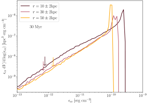
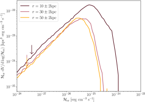
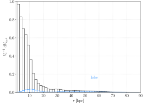
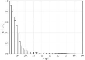
Figure 9: Weighted volume distributions and filling factors of the CR energy density $\epsilon_{\mathrm{cr}}$ and the Alfvén heating rate $\mathcal{H}_{\mathrm{cr}}$ of our fiducial simulation at $30\ \mathrm{Myr}$. We show the weighted volume distribution of CR energy density $\epsilon_{\mathrm{cr}}\mathrm{d}V/\mathrm{d}\log(\epsilon_{\mathrm{cr}})$ (top left) and CR heating rate density $\mathcal{H}_{\mathrm{cr}}\mathrm{d}V/\mathrm{d}\log(\mathcal{H}_{\mathrm{cr}})$ (top right), which characterize the isotropy of our CR distribution. The arrows mark the minimum CR energy density and heating rate density necessary to cover $3\sigma$ (99.8%) of the CR energy and heating power at that radius, respectively. Due to their similarity, we adopt a common value for the floor values $\epsilon_{\mathrm{cr,min}}=10^{-12}\ \mathrm{erg}\ \mathrm{cm}^{-3}$ and $\mathcal{H}_{\mathrm{cr,min}}=3\times 10^{28}\ \mathrm{erg}\ \mathrm{cm}^{-3}\ \mathrm{s}^{-1}$ at all radii. In the bottom panels, we show the filling factor of $\epsilon_{\mathrm{cr}}$ and $\mathcal{H}_{\mathrm{cr}}$ for cells above these thresholds. Note that we suppress heating rates inside bubbles. The filling factor of the lobes ($X_{\mathrm{jet}}>10^{-3}$) is overplotted in the bottom left panel. The small filling factor of the lobes highlights the importance of CR diffusion to isotropize CRs. The large volume filling factor of $\epsilon_{\mathrm{cr}}$ and $\mathcal{H}_{\mathrm{cr}}$ becomes evident for $r\lesssim 15\ \mathrm{kpc}$, suggesting that CR heating is isotropic at small radii.

4.2 Mixing

In order to analyse the mixing efficiency for different magnetic field configurations, we use a suite of simulations without CRs (bottom in Table 1) to solely focus on magnetic effects. As discussed in the previous section, the effect of draping stabilises the bubble against early disruption from interface instabilities. However, the draping layer only suppresses the growth of wave modes along the direction of the mean field but not perpendicular to it. As the bubble rises in the cluster potential, its surface is constantly warped and twisted by the turbulence, which causes incomplete alignments of the external turbulent magnetic field with respect to the bubble surface. Possibly, magnetic fields also cancel out through numerical magnetic reconnection. These effects likely compromise the effects of draping temporarily for our complex simulations in comparison to idealised setups. In addition, we model the effect of helical fields, which develop in the turbulent bubble from the initially toroidal fields in the jet and also show stabilising effects (Ruszkowski et al., 2007).

The simulations in the top left panel of Fig. 6 show a case with internal helical and external turbulent fields, two cases with either one of the two field configurations and one without any magnetic fields. Visually the morphology of the simulations including magnetic fields appear similar to the ones without (accounting for projection effects). However, the density contrast within the lobes is smaller in the simulation without magnetic fields, indicating that mixing is suppressed by either the helical lobe field and/or draped external fields. This can also be seen in the top right panel of Fig. 6, where we show the volume covered by a given jet mass fraction $X_{\mathrm{jet}}$. Initially, the distribution peaks at $X_{\mathrm{jet}}=1$ and if the bubble was perfectly insulated the distribution would stay there. The faster the distribution moves to lower values of $X_{\mathrm{jet}}$, the more efficiently does the bubble material mix with the ICM. Conversely, a slow evolution indicates a significant suppression of mixing. Accounting for magnetic fields in the ICM, which enables magnetic draping, shifts the filling factor to higher values of $X_{\mathrm{jet}}$ indicating an insulating effect of draping and preventing fast mixing. In reality, this suppression of mixing should be even higher as the driven external turbulence is weaker in the case without magnetic fields in comparison to the case of ICM magnetic fields (see Section 2) since turbulence amplifies mixing (e.g., Ogiya et al., 2018).

Similarly, our simulation with purely internal helical magnetic fields suppresses mixing in comparison to the case without B. This suggests that our case with internal and external fields should show an even smaller degree of mixing in comparison to either of the two individual cases with a single magnetic component. However, there is only a slightly smaller jet mass fraction retained in this double-magnetic case in comparison to the internal field case (Fig. 6). The loss of stability in the case of the additional draping layer can be explained with the increase in driven external turbulence for a magnetized ICM.

In the lower left panel of Fig. 6, we compare runs with constant jet lifetime ($\tau_{\mathrm{jet}}$) but varying jet power ($P_{\mathrm{jet}}$). We find a decrease in the mixing efficiency for jets with higher power in agreement with Brüggen et al. (2002). Our normalisation ensures comparability across differently sized lobes. The high-power jets penetrate the inner region of the ICM as highly collimated outflows. Their disruption occurs further out in the cluster atmosphere where the magnetic fluctuations and thereby the level of turbulence is lower. This environment impedes mixing in comparison to low-power jets which get disrupted inside the highly turbulent cluster centre. In addition, Rayleigh Taylor instabilities should arise later for larger cavities (higher power jets at constant $\tau_{\mathrm{jet}}$) as the growth time scale of the instability increases for larger scales. This argument is confirmed when we compare simulations with varying $\tau_{\mathrm{jet}}$, but constant jet power (lower-right panel Fig. 6). Here, the larger cavities (larger $\tau_{\mathrm{jet}}$) remain more stable. We conclude that less energetic jets (decreased $P_{\mathrm{jet}}$ or $\tau_{\mathrm{jet}}$) show increased mixing efficiencies of lobes with the ICM.

5 Cosmic ray evolution

After discussing the magnetic structure at the rising bubbles, we now turn our attention to the distribution of CRs. First we examine the diffusive transport of CRs and then detail Alfvén wave heating by CRs.

5.1 CR diffusion and streaming

As discussed in Section 2.3, we model active CR transport via the anisotropic diffusion approximation to emulate CR streaming (see also Sharma et al., 2009). To this end, we include CR energy losses through Alfvén cooling and adopt a constant parallel diffusion coefficient ($\kappa_{\parallel}=10^{29}\ \mathrm{cm}^{2}\ \mathrm{s}^{-1}$) so that it approximately matches the instantaneous CR diffusion coefficient $\kappa_{\mathrm{cr,A}}\equiv{}l_{\mathrm{cr}}v_{\mathrm{A}}$ in the ICM.

This choice for $\kappa_{\parallel}$ is examined in Fig. 7, which shows projections of thin layers of different quantities related to CR transport. As expected, the CR population has a large CR gradient length $l_{\mathrm{cr}}$ in the bubble (except for the boundary) as the CR population quickly reaches a homogeneous distribution for our choice of $\kappa_{\parallel}$. Outside the bubble, $l_{\mathrm{cr}}$ drops quickly. The behaviour is echoed by the Alfvén velocity $v_{\mathrm{A}}$: inside the jet (and bubble) it attains values up to $10^{4}\ \mathrm{km}\ \mathrm{s}^{-1}$ owing to the low density and comparably large magnetic field whereas it fluctuates around a value of $10^{2}\ \mathrm{km}\ \mathrm{s}^{-1}$ in the ICM. The distribution of Alfvén cooling times, $t_{\mathrm{A}}=l_{\mathrm{cr}}/v_{\mathrm{A}}$, is a direct consequence of this: $t_{\mathrm{A}}$ drops from values of $\approx 1$ Gyr inside the bubbles to values ranging from 10$-$30 Myrs, comparable to typical jet duty time scales (e.g., Vantyghem et al., 2014; Turner, 2018).

The combination of high $v_{\mathrm{A}}$ and $l_{\mathrm{cr}}$ inside the bubble leads to a large value of the instantaneous CR diffusion coefficient $\kappa_{\mathrm{cr,A}}\approx 10^{32}\ \mathrm{cm}^{2}\mathrm{s}^{-1}$. While this is much larger than our adopted constant diffusion coefficient of $10^{29}\ \mathrm{cm}^{2}\mathrm{s}^{-1}$, the CR distribution in the bubble is already homogeneous as can be seen in the CR energy density in Fig. 3; increasing $\kappa_{\parallel}$ further would not alter our results. Outside the bubble, the diffusion coefficient drops by three orders of magnitude to $\kappa_{\mathrm{cr,A}}\approx 10^{29}\ \mathrm{cm}^{2}\mathrm{s}^{-1}$. There, the CRs are magnetically unconfined and the value of the diffusion coefficient becomes crucial for accurately capturing the dynamics, justifying our choice of $\kappa_{\parallel}$.

The small CR length scale $l_{\mathrm{cr}}$ at the bubble interface combined with a high Alfvén velocity decreases the Alfvén cooling time $t_{\mathrm{A}}$ significantly to values of order 1 Myr. This would increase the Alfvén heating rate at the edges and drain a significant amount of CR energy from the bubble. In reality, the CR gradient would instead be smoothed out on the short Alfvénic crossing time across the jet and stay flat during inflation of the bubble and its evolution thereafter. This explains our initial choice of limiting Alfvén cooling to regions outside the bubble ($X_{\mathrm{jet}}<10^{-3}$) as a numerical safeguard to prevent numerically-induced CR cooling.

We discuss in Section 4 that CRs can only escape through the lower part of the bubble. As they are conducted out of the bubble they remain confined to the magnetic field. Consequently, the vertically oriented, magnified magnetic field lines are traced by the Alfvén heating rate. This demonstrates the importance of simulating the exact structure of the magnetic field in the vicinity of the bubble. It will be interesting to see how substructure induced motions and radiative cooling influence this result.

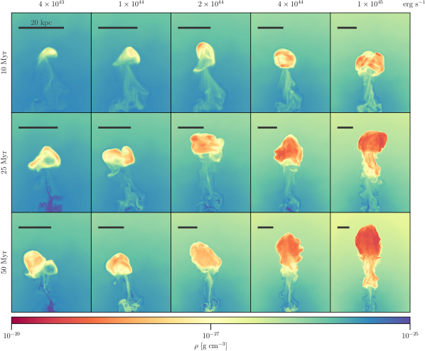
Figure 10: Density projections for our lower resolution simulations with varying jet parameters. We show a full projection of the jet tracer-weighted density at 70 Myr. The jet activity time increases from top to bottom and the jet power increases from left to right as indicated. Jets with similar energy are ordered along diagonals from the bottom left to the top right. The scale bar corresponds to $20\ \mathrm{kpc}$ in all panels and decreases from left to right but stays constant along diagonals with $E_{\mathrm{jet}}\approx\mathrm{const}$.

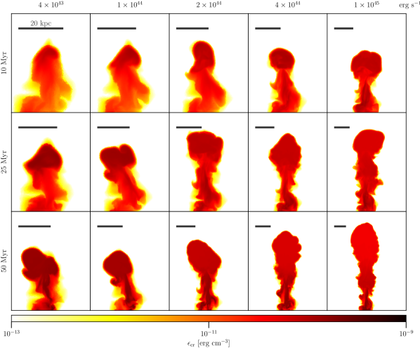
Figure 11: Same as in Fig. 10 but for the jet tracer-weighted CR energy density $\epsilon_{\mathrm{cr}}$. Even for bubbles with low density contrast (top left) there is significant CR energy density released into the ICM.

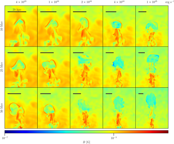
Figure 12: Same as in Fig. 10 but for the jet tracer-weighted magnetic field strength $B$. The red envelope surrounding the bubbles clearly show magnetic draping and magnetic fields in the wake of bubbles are strongly amplified. Note that the weighting procedure enhances the magnetic field in the wake of the bubble.

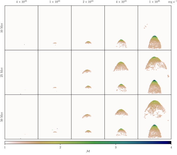
Figure 13: Same as in Fig. 10 but for the Mach number $\mathcal{M}$ that was weighted with the energy dissipation rate at the shocks. We overplot $\mathcal{M}$ projections of two snapshots, at $5\ \mathrm{Myr}$ and $20\ \mathrm{Myr}$. Here, projections have constant dimensions of $80\ \mathrm{kpc}\times 60\ \mathrm{kpc}\times 60\ \mathrm{kpc}$ centred at (40-0-0). Low-power jets show at best small Mach numbers whereas the Mach numbers of high power-jets decrease quickly with time. These characteristics are in agreement with observations of FRI and FRII, respectively.

5.2 CR distribution and Alfvén wave heating

In Fig. 8 (upper left panel) we show the radial profile of the Alfvén heating rate ($\mathcal{H}_{\mathrm{cr}}$) of our fiducial model at different times during and after the jet lifetime $\tau_{\mathrm{jet}}=25$ Myr. In agreement with our sub-grid model of CR Alfvén cooling in bubbles and in order to focus solely on the heating of the ICM, we impose a jet tracer threshold of $X_{\mathrm{jet}}<10^{-3}$ to exclude artificially high cooling rates within the bubble. The result is robust up to factors of two when we vary the jet tracer threshold by an order of magnitude. We compare our simulated Alfvén heating rates to theoretical predictions by Jacob & Pfrommer (2017a) for the Perseus cluster who found steady-state solutions in which the heating rates due to Alfvén heating (at small radii) and thermal conduction (at larger radii) balance radiative cooling. Our simulated Alfvén heating rates are in good agreement with the theoretical predictions up to $30\ \mathrm{Myr}$ after jet launch with details depending on parameter choices as we will now discuss. At later times, newly launched jets are expected to replenish the CR energy reservoir, which has then significantly cooled via Alfvén wave losses.

The overall shape of the radial profile of $\mathcal{H}_{\mathrm{cr}}$ is determined by the jet energy, power and lifetime. For efficient CR heating in the centre of clusters, the exact value of the jet energy $E_{\mathrm{jet}}$ proves to be crucial: if it is too small there is not enough CR energy injected and the induced heating rate cannot balance radiative losses of the gas. On the other hand, if the jets are too energetic they pierce out of the cluster centre and reach the outskirts of the core, which makes it difficult for CRs to diffuse back to the origin and to maintain a large heating rate.

For jets with $E_{\mathrm{jet}}=\mathrm{const.}$ but varying luminosity and lifetime, the profiles differ slightly (Fig. 8, top right panel). The heating rate profile is steeper for low-luminosity jets with longer activity times. This is because low-luminosity jets are more quickly decelerated by the inertia of the ambient ICM and CRs have more time to diffuse back towards the cluster centre where they sustain a larger central heating rate.

Jets with constant $\tau_{\mathrm{jet}}$ exhibit an increasing heating radius with increasing $P_{\mathrm{jet}}$ (Fig. 8, bottom left panel). A larger jet luminosity corresponds to enhanced CR production (at $\tau_{\mathrm{jet}}=\mathrm{const.}$) while the jet also pushes to larger radii. At small radii there is a larger variance of $\mathcal{H}_{\mathrm{cr}}$ because of the fast CR transport to large radii in the jet which competes with the backwards CR diffusion and advection towards the dense cluster centre. Jets with $P_{\mathrm{jet}}=\mathrm{const.}$ produce almost self-similar $\mathcal{H}_{\mathrm{cr}}$ profiles that scale with the amount of injected CR energy (Fig. 8, bottom right panel).

A successful heating mechanism in CC clusters is not required to act isotropically throughout the entire core region. However, as cooling material falls to the centre, eventually it should be heated at some inner radius (McNamara & Nulsen, 2012), which poses requirements for the isotropy of the proposed heating mechanism at small radii. To examine the volume-filling of CR heating in our simulations, we first show the volume distributions of CR energy density and Alfvén-heating rate in the top panels of Fig. 9. Diffusion leads to a shallow CR floor in the cluster centre and beyond at later times. To quantify the degree of CR isotropy, we define a minimum amount of the CR energy density and Alfvén heating rate by requiring that 3$\sigma$ (99.8%) of CR energy and Alfvén heating power are above these floor values, respectively.

For each concentric shell of radius $r$, we display the volume fraction covered by cells with $\epsilon_{\mathrm{cr}}$ (or $\mathcal{H}_{\mathrm{A}}$) above these floor values and normalise it to the volume of the shell at this radius (bottom panels of Fig. 9). While the bipolar jets transport CRs mainly along the jet axes, subsonic CR advection and diffusion strongly limit lateral transport of CRs within a CR cooling time at large radii ($r\gtrsim 15\ \mathrm{kpc}$), precluding isotropic heating there. In contrast, Alfvén-wave heating is almost isotropic at small radii ($r<15\ \mathrm{kpc}$).

In fact, observations favour a smooth heating process with only minimal temporal over-heating or -cooling (Fabian, 2012). Our simulations reproduce this property as we deduce from the evolution of the pressure and temperature profiles in Fig. 1. The profiles show little variance after the initial perturbation in temperature and density due to the propagating jet at $10\ \mathrm{Myr}$.

The match of $\mathcal{H}_{\mathrm{cr}}$ in our simulations to the steady-state solutions (Jacob & Pfrommer, 2017a) validates that dynamically evolved jets with plausible parameters can distribute CRs sufficiently well to successfully balance the radiative cooling losses of the ICM via CR heating on timescales $t\lesssim 30$ Myr. Future simulations including gas cooling and jet injection coupled to accretion will scrutinise the feasibility of the model on long timescales and whether it is self-regulating.

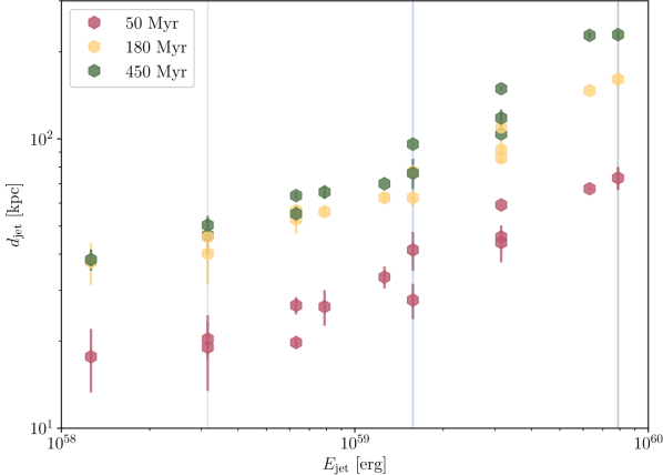
Figure 14: Distance of jet travel vs. jet energy of our lower resolution simulations. The jet distance $d_{\mathrm{jet}}$ for individual jets is defined as the distance from the SMBH to the point to which half the jet mass $X_{\mathrm{jet}}m$ (of the upper hemisphere) has travelled (typically situated inside the lobe). We show the average distances of the upper and lower jets for every individual simulation (hexagons) and the error bar denotes the ranges for the two individual jets. There is a clear correlation of jet distance and energy at each of the three different simulation times (indicated by colour). The vertical (light blue) lines correspond to the three simulations shown in the left panel of Fig. 15.

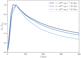
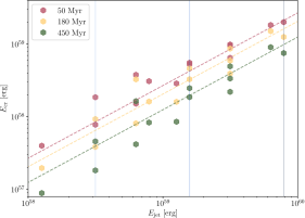
Figure 15: The evolution of the total CR energy as a function of jet energy for three different jet luminosities of our lower resolution simulations. On the left, we show the CR energy $E_{\mathrm{cr}}$ as a function of time normalised to its maximum value $E_{\mathrm{cr,0}}$. During the jet stage, the CR energy increases steadily until $\tau_{\mathrm{acc}}$ after which it decreases as a result of escaping CRs that suffer Alfvén wave losses in the ICM. On the right, we show the CR energy $E_{\mathrm{cr}}$ as a function of total jet energy $E_{\mathrm{jet}}$ for different simulations at three different times (colour coded). A linear fit to each of the three simulation times is shown with dashed lines and describes the simulations well. The significant scatter towards small jet energies corresponds to the increased mixing efficiency for these systems. The vertical (light blue) lines correspond to the simulations shown in the left panel.

6 Parameter study

The following parameter study focuses on jet power and lifetime. Here, we will show that instead of these two parameters, jet energy appears to be the most important parameter for determining jet morphology, CR distribution and magnetic field structure, whereas the jet power determines the maximum attainable Mach number.

6.1 Bubble morphology

In Fig. 10, we show how the bubble morphology changes with varying jet parameters at 70 Myr. While the jet acceleration of CRs in our subgrid model is still ongoing for jets in the bottom row, the resulting dynamical effects of this late-time acceleration ($t>\tau_{\mathrm{jet}}$) are negligible. Jet lifetime increases from top to bottom and jet power increases from left to right. Jets with similar energy are ordered along diagonals from the bottom left to the top right. In order to identify the highly anisotropic features of the bubble, Figs. 10, 11, and 12 show projections weighted with the jet tracer mass fraction $X_{\mathrm{jet}}$. Additionally, we show in Fig. 13 the Mach number $\mathcal{M}$ weighted with the energy dissipation rate at the shocks. Note that we assign a minimum value of $X_{\mathrm{jet}}=10^{-10}$ to every cell to also display the background. The projection depth corresponds to the projection width.

We see that jet energy is responsible for setting the overall bubble morphology. Bubbles inflated with a low-power jet with a long activity time resemble bubbles originating from jets with high power but shorter lifetimes. In Fig. 14, we show the mean distance travelled by the jet as a function of the jet energy at three different times. We find a power-law relation $d_{\mathrm{jet}}\propto E_{\mathrm{jet}}^{\alpha}$ with $\alpha\approx 0.4$. Jets with the same energy reach similar heights, confirming the correlation. Because different jets with $E_{\mathrm{jet}}=\mathrm{const.}$ produce bubbles of similar sizes, this implies comparable Rayleigh-Taylor lifetimes (see Section 4.2).

Low-energy jets inflate smaller lobes (Fig. 10, to the upper left), which terminate at lesser heights. They are deflected from their original jet trajectories and show clear signs of ongoing mixing (as indicated by the low density contrast with the ICM). These are the signatures of FRI-type jets according to the Fanaroff-Riley (FR) classification (Fanaroff & Riley, 1974). Increasing jet energy (top left to bottom right) results in jets that penetrate the ICM to larger distances from the cluster centre. They propagate mostly along the original jet direction and can sustain high-density contrasts for longer times. These properties resemble jets of the FRII-type category.

Producing realistic FRI jets in simulations requires resolving the radius of the jet with $\approx 10$ cells (Anjiri et al., 2014), which is difficult to achieve in our large-scale simulations for our low-power jet models. In these idealised jet simulations the occurrence of low-power FRI-type jets is then attributed to the development of a turbulent structure rather then terminal shocks as in the case of high-power FRII jets. The jet power that marks a threshold between these jet categories is given by $P_{\mathrm{jet}}\sim 10^{43}\ \mathrm{erg}\ \mathrm{s}^{-1}$ according to simulations (Massaglia et al., 2016). Here, we can confirm that FRI-like jets are obtained in our simulations, albeit at a somewhat higher threshold luminosity. We address this point in Appendix B and find that while this threshold luminosity decreases with increasing numerical resolution, general properties regarding distribution of magnetic fields, CRs and heating rates remain qualitatively similar. Most importantly, we find that jet energy appears to be the leading variable to distinguish between the main FR jet features. Alternative scenarios for the origin of FRI jets include de-focusing due to a magnetic kink instability in the jet (Tchekhovskoy & Bromberg, 2016), mixing due to Kelvin-Helmholtz instabilities in sheared relativistic flows (e.g., Perucho et al., 2010) and mass entrainment from stellar winds (e.g., Wykes et al., 2015).

We leave detailed morphological studies of bubbles in cooling clusters that are generated through the interplay of accretion and jet launch for future studies. Additionally, the interaction of subsequent generations of bubbles may play a key role as they may merge and form large outflowing cavities (Cielo et al., 2018). Finally, the jet lifetime cannot be arbitrarily increased to form ever larger bubbles as these will inevitably fragment, generating multiple disconnected bubbles in a turbulent environment (Morsony et al., 2010).

6.2 CR distribution

Looking at the distribution of CR energy density, $\epsilon_{\mathrm{cr}}$, in Fig. 11, it becomes apparent that $\epsilon_{\mathrm{cr}}$ is more homogeneous than the density across our models. This means that even if there is no visible cavity due to low contrast in X-rays, there may still be a substantial CR population that is responsible for efficient Alfvén wave heating.

The previously described trend that low-energy jets form bubbles that are easily deflected and dispersed early-on translates to a very centrally localised CR distribution with a high degree of isotropy (Fig. 11). Conversely, high-energy jets develop bubbles that stay intact out to large distances. CRs continuously diffuse out of the bubble but the majority of the CR energy is transported to large radii. This makes low-energy jets more efficient in heating the fast-cooling cluster centres. These low-energy systems have a larger mixing efficiency and their bubbles remain in the central regions of the cluster (Mukherjee et al., 2016).

The sequence of CR acceleration, bubble disruption, diffusive CR escape, and successive Alfvén cooling is expected to reflect on the available CR energy for individual jets (Fig. 15). Interestingly, we observe a linear correlation between CR energy and the total jet energy. When considering a sample of jets with the same energy, the jet with the longest lifetime $\tau_{\mathrm{jet}}$ will accelerate CRs for longer periods of time. As CRs cool over time, the low-power (high-lifetime) jet is expected to maintain a larger CR energy, which explains the scatter at constant energy in Fig. 15.

Another source of scatter in the linear relation is due to the difference in mixing efficiency for jets with variable jet power. The left panel of Fig. 15 exemplifies this point as it shows the normalised CR energy for jets with constant lifetime but varying jet power. During the jet stage, the CR energy increases as kinetic energy is dissipated and transferred to CR energy until $\tau_{\mathrm{acc}}$. Afterwards, CR energy decreases as a result of escaping CRs that suffer Alfvén wave losses in the ICM. A decrease in jet power implies a decrease of CR energy in the entire cluster. As discussed in Section 4.2, low-power jets mix more efficiently, which results in earlier disruption times of the lobe and thereby an earlier onset of CR cooling.

6.3 Magnetic field structure

The magnetic field structure shows the draping layer wrapped around the bubbles in most of the different jet simulations (Fig. 12). Even though the draping layer lies outside the bubble interface with the ambient ICM, the numerically diffused advective jet tracers still highlight this feature. Consequently, the jet tracer-weighted projection leads to apparent amplification ratios of $>2$. However, the actual ratios are on the order of $\sim 2$ as discussed in Section 4.1. In some exceptional cases, the draping layer remains absent. This is due to the turbulent nature of the ICM that causes perturbations in the trajectory of the bubble and generates a corrugated bubble interface as the bubble expands into a region of lower ambient pressure. The local change of propagation direction forces the bubble to accumulate a new draping layer. In addition, numerical reconnection of magnetic field lines in the turbulent environment may temporarily erase the draping layer as fields of different polarity accumulate in the layer.

We observe strongly amplified magnetic filaments in the wakes of every bubble, which reach field strengths up to 30 $\mu$G. These elongated filaments align approximately along the jet axis and point back to the cluster centre to which they conduct the diffusing CRs. These strongly magnetised magnetic structures resemble observed H$\alpha$ filaments in CC clusters.

As we have seen, a large fraction of the jet tracers is mixed with the ICM in the wake of the jet. This causes the magnetic field in the region to be significantly enhanced compared to the surrounding magnetic field. Due to this effect the contrast in magnetic field strength between wake region and ICM increases for larger projection box sizes (bottom right of Fig. 12).

6.4 Shocks and Mach numbers

Most observed Mach numbers of expanding lobes that reside in CC clusters are observed to be at the order of $\mathcal{M}\sim 1$ (McNamara & Nulsen, 2007). Using a shock finder in arepo (Schaal & Springel, 2015), we detect and characterise the bow shock that is driven into the ICM by the propagating lobes. In Fig. 13, we show projections of the Mach numbers of this bow shock, weighted with the energy dissipation rate at two different times, at 5 Myr and 20 Myr.

The shock strength scales with the jet power as expected. At $5\ \mathrm{Myr}$, the lobes of low-power jets ($\leq 2\times 10^{44}\ \mathrm{erg}\ \mathrm{s}^{-1}$) predominantly exhibit Mach numbers $\mathcal{M}\lesssim 1.5$, similar to observations. In contrast, the lobes of high-power jets ($>2\times 10^{44}\ \mathrm{erg}\ \mathrm{s}^{-1}$) exhibit strong Mach numbers $\mathcal{M}>4$. However after $20\ \mathrm{Myr}$ those have already decreased to values of $\mathcal{M}\sim 2-3$. After the jet is switched off, only individual cells exhibit Mach numbers $\mathcal{M}>1$. Thus, even our lobes from high-power jets only exhibit high Mach numbers for a short period of time and low-to-intermediate Mach numbers for most of the time the jet is active. We conclude that our simulations successfully reproduce the observed low Mach numbers for the lobes of low-power jets.

7 Conclusions

Using 3D MHD simulations with the moving-mesh code arepo, we study the evolution of magnetised and CR-filled jets in an idealised Perseus galaxy cluster. Following the jet-driven inflation of underdense bubbles, we study their buoyant rise in the cluster atmosphere and how they interact with a turbulent cluster magnetic field. The bubbles are exposed to interface instabilities which finally disrupt the bubbles and enable initially confined CRs to diffusively escape and to heat the ambient ICM. Here we summarise our main findings:

• The accumulation of magnetic fields at the bubble interface as a result of buoyant bubble motion relative to the ambient ICM stabilises the bubble against the turbulent environment, suppresses Kelvin-Helmholtz instabilities, and reduces the mixing efficiency. Internal helical magnetic fields show a similar effect.

• We find that a decrease in jet power and/or in total jet energy increases the mixing efficiency of the jet.

• CRs inside the bubbles are confined by the draped magnetic field that inhibits diffusion across the bubble surface.

• In the wake of the bubble, the magnetic field is strongly amplified and adiabatically compressed by converging inflows that are compensating the upwards motion of the bubble. Differential motions stretch the magnetic field so that it becomes filamentary and aligned along the jet axis. These strongly magnetised filaments acquire strengths of 30 $\mu$G and resemble observed H$\alpha$ filaments in clusters. We postpone a detailed study to future work.

• These radial magnetic filaments connect the bubble interior to the ambient ICM, and allow CRs to diffusively escape into the ICM and heat the surrounding medium. Our simulated radial profiles of the CR-induced Alfvén wave heating rate match CR heating rates predicted by steady-state models of CC clusters extremely well (Jacob & Pfrommer, 2017a). Inside a radius $r\lesssim 15$ kpc, we find a volume-filling CR distribution that generates isotropic Alfvén wave heating, which is necessary for solving the cooling flow problem at the centres of clusters. The temporal evolution varies significantly such that time-dependent modeling becomes crucial.

• A parameter study of different jet simulations with varying jet lifetime and jet power reveals that the jet energy is the critical parameter for determining the overall bubble morphology and CR distribution. Magnetic draping as well as the strong filamentary magnetic field amplification in the wakes is ubiquitous in our sample.

• We find a high degree of coherence and decreasing mixing efficiency with increasing jet energies. This finding and the observed low Mach numbers show that we can reproduce the main features of both, FRI and FRII-like jets: FRII jets exhibit bipolar, lobe-brightened morphologies with high density contrasts that power high Mach numbers $\mathcal{M}\sim 4$ in the ICM at early times. On the other hand, FRI jets are characterized by lower density contrasts, show more deflected and corrugated bubbles that generate a laterally more expanded CR distribution at the centre, and do not drive detectable shocks into the ICM.

These results encourage further studies of the impact of CR-filled AGN bubbles on radiatively cooling CC cluster atmospheres. Accounting for accretion onto SMBHs and successive jet formation will enable us to find out whether we can obtain a self-regulated CR heating-radiative cooling cycle.

Appendix A Magnetic Field Generation

The external turbulent magnetic field follows a Kolmogorov spectrum in agreement with observations (Bonafede et al., 2010; Kuchar & Enßlin, 2011). The generation of the initial conditions for the magnetic field follows largely Appendix A in Ruszkowski et al. (2007). The Gaussian-distributed random magnetic field with vanishing mean ($\langle\textbf{{B}}\rangle=\mathbf{0}$ but $\sqrt{\langle\textbf{{B}}^{2}\rangle}\neq 0$) is set up with a Kolmogorov power spectrum in Fourier space. The magnetic field is scaled to ensure a shell-averaged constant magnetic-to-thermal pressure ratio $X_{B,\mathrm{ICM}}=P_{B}/P_{\mathrm{th}}$ throughout the cluster. The three components of the magnetic field $B_{i}$ ($i\in\{1,2,3\}$) are treated independently to ensure that the final distribution of $\textbf{{B}}(\textbf{{x}})$ has a random phase. The large discrepancy between minimum cell size and computational box size necessitates the interpolation of fields from multiple nested Cartesian grids with increasing resolution onto our initial setup.

First, we compute Gaussian-distributed field components that obey a one-dimensional power spectrum $P_{i}(k)$, given by $P_{i}(k)\propto k^{2}|\tilde{B}_{i}(k)|^{2}$, with

$$|\tilde{B}_{i}(k)|^{2}=\begin{cases}A,&k<k_{\mathrm{inj}},\\ A\left(\dfrac{k}{k_{\mathrm{inj}}}\right)^{-11/3},&k_{\mathrm{inj}}\leq k,\end{cases}$$ (5)

where $A$ is a normalisation constant, $k=|\textbf{{k}}|$, and $k_{\mathrm{inj}}$ is the injection scale of the field. Modes on large scales ($k<k_{\mathrm{inj}}$) follow a random white-noise distribution while modes in the inertial range ($k>k_{\mathrm{inj}}$) obey a Kolmogorov power spectrum. For each magnetic field component, we set up a complex field such that

$$[\Re(\tilde{B}_{i}(\textbf{{k}})),\Im(\tilde{B}_{i}(\textbf{{k}}))]=[G_{1}(\Lambda_{1},\Lambda_{2},\sigma_{k}),G_{2}(\Lambda_{1},\Lambda_{2},\sigma_{k})],$$ (6)

where $\Lambda_{1}$ and $\Lambda_{2}$ are uniform random deviates so that the function $G_{i}(\Lambda_{1},\Lambda_{2},\sigma_{k})$ ($i\in\{1,2\}$) returns Gaussian-distributed values with standard deviation $\sigma_{k}=\tilde{B}_{i}$ for every value of $k$. We then normalise the spectrum to the desired variance of the magnetic field components in real space, $\sigma_{B}$ using Parseval’s theorem,

$$\sigma_{B}^{2}=\dfrac{1}{N^{2}}\sum_{i}\sum_{k_{j}}|\tilde{B}_{i}(k_{j})|^{2}.$$ (7)

To eliminate overlapping magnetic field lines between different nested meshes, we (i) reorient radial field lines in the overlap region and (ii) remove the inner part of our coarser mesh via a spherical tapering function and replace it with the tapered high-resolution mesh. Since this process introduces divergences in the magnetic field, we iteratively perform divergence cleaning steps while accounting for the reorientation of radial magnetic field:

1. Divergence cleaning in Fourier space. We eliminate the field component in the direction of $\bm{k}$, via the projection operator:

   $$\tilde{\textbf{{B}}}\to\tilde{\textbf{{B}}}-\hat{\textbf{{k}}}(\hat{\textbf{{k}}}\cdot\tilde{\textbf{{B}}})$$ (8)

   in order to fulfil the constraint $\bm{\nabla}\mathchoice{\mskip 3.0mu\lower 0.86108pt\hbox{\scalebox{1.5}{$\cdot$}}\mskip 3.0mu}{\mskip 3.0mu\lower 0.86108pt\hbox{\scalebox{1.5}{$\cdot$}}\mskip 3.0mu}{\lower 1.29167pt\hbox{\scalebox{1.2}{$\cdot$}}}{\lower 1.29167pt\hbox{\scalebox{1.2}{$\cdot$}}}\textbf{{B}}=0$.

2. Field rescaling to constant $X_{B,\mathrm{ICM}}$. We rescale the magnetic field to obtain a constant average value of $\langle{}X_{B,\mathrm{ICM}}(r)\rangle$ in thin concentric shells of radius $r$ around the cluster centre.

3. Cleaning and smoothing transition regions between meshes. In order to prevent interconnecting field lines between meshes, we force the radial magnetic field lines to bend in the overlap regions of different meshes. To this end, we remove the radial component of the magnetic field in real space via

   $${\textbf{{B}}}\to\left[1-g(r)\hat{\textbf{{r}}}\hat{\textbf{{r}}}\right]{\textbf{{B}}}$$ (9)

   where $\hat{\textbf{{r}}}$ is the unit radial vector and

   $$g(r)=1-\left|\cos\left(\frac{\pi}{2}\frac{x+\Delta x-1}{\Delta x}\right)\right|$$ (10)

   for $1-\Delta x<x<1+\Delta x$ with $x=r/r_{\textrm{m}}$ and $\Delta x=0.05$. The overlap radius of the two meshes is given by $r_{\mathrm{m}}$.

   Afterwards, we taper the field strength in the overlapping regions of one mesh with a spline $f_{S}(x)=0.5\cos\left(\pi(r-r_{m})/d_{m}\right)$, where the taper width $d_{m}$ is set to the larger (outer) cell size of the two adjacent meshes. Its neighbouring mesh uses the spline $f_{C}(x)=1-f_{S}(x)$.

   Steps (i)-(iii) are repeated until the divergence of the magnetic field has sufficiently decreased. The resulting field is interpolated on our adaptive, smoothly varying mesh in the initial conditions, which are setup in hydrostatic equilibrium. To maintain this equilibrium, the temperature is varied according to

   $$nk_{\mathrm{B}}\delta T=-\frac{\delta\bm{B}^{2}}{8\pi}.$$ (11)

   Finally, we relax the mesh with arepo so that a remaining (small) divergence is cleaned with the Powell algorithm. To reverse the decrease of the magnetic field strength due to the conversion from magnetic to turbulent energy, we rescale the magnetic field with a constant factor and obtain $X_{B,\mathrm{ICM}}$.

Appendix B Resolution study

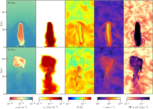
Figure 16: Same model as in Fig. 3 at lower resolution with projection dimensions $80\ \mathrm{kpc}\times 50\ \mathrm{kpc}\times 4\ \mathrm{kpc}$. Because magnetic tension is less well resolved and more affected by numerical diffusion, the external magnetic field strength and turbulent motions are smaller in amplitude. Moreover, at lower numerical resolution the velocity gradient at the jet foot is not sufficiently resolved, which implies that the jet does not travel as far as for the high-resolution simulation. Thus, momentum transport is less efficient here.

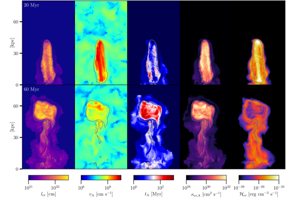
Figure 17: Same model as in Fig. 7 at lower resolution with projection dimensions $80\ \mathrm{kpc}\times 50\mathrm{kpc}\times 4\ \mathrm{kpc}$. The exact distribution of CRs depends somewhat on resolution because jet the distance of jet travel increases with numerical resolution. However, the quantities related to CR transport ($\kappa_{\mathrm{cr,A}}$ and $\mathcal{H}_{\mathrm{cr}}$) show general agreement with our high-resolution simulation.

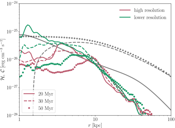
Figure 18: Comparing the Alfvén-wave heating rate due to streaming CRs for our low- and high-resolution simulations at $t=20$, 30 and 50 Myr (see also Fig. 8). While the jet in the high-resolution simulation propagates further, the CR heating rate drops slightly in the cluster centre by a factor of less than two.

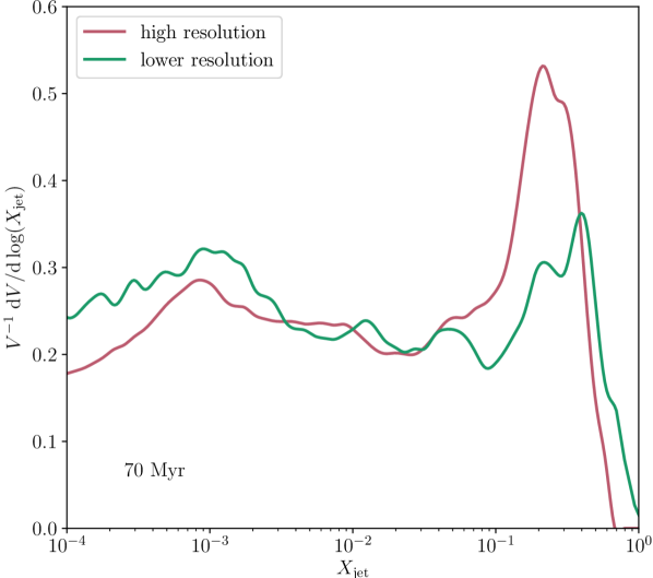
Figure 19: Comparing the mixing efficiency of the bubble for CR simulations at different numerical resolutions (cf. Fig. 6). To ensure an unbiased comparison we show the normalised filling factor of a given jet mass fraction $V^{-1}\ \mathrm{d}V/\mathrm{d}\log(X_{\mathrm{jet}})$. Mixing is suppressed at higher resolutions due to the more compact jet that propagates to larger distances. The lines are smoothed for clarity.

To test numerical convergence, we compare simulation runs with the fiducial jet parameters at high and lower resolution (cf. Table 2). The overall evolution (Fig. 16) of the jet remains qualitatively similar. However there are (smaller) quantitative differences such as the emergence of Kelvin-Helmholtz instabilities on the jet surface in our high-resolution simulation. That instability remain dynamically subdominant as the more dominant Rayleigh-Taylor instability starts to develop. However, the magnetic field strengths in the ICM remain larger for longer time scales in comparison to the run at fiducial resolution since we better resolve magnetic tension due to the lower level of numerical diffusion. This increased level of magnetic turbulence causes the bubble to change direction more often at late times.

As discussed in Weinberger et al. (2017), the distance travelled by the jet is resolution dependent. For this, resolving the velocity structure of the jet proves crucial. The jet expands more laterally at lower resolution as the prescribed jet width used for all simulations is insufficient to resolve the velocity gradient of the jet. The jet compensates by broadening. This spreads the area of the effective momentum leading to a decrease of the jet velocity and thus a smaller distance travelled at lower resolution. However, the properties of CRs remain robust against changes in resolution (Fig. 17 vs. Fig. 7 ).

Figure 18 compares radial profiles of the Alfvén heating rate for our fiducial and high-resolution simulations. Because better resolved jets travel further, the Alfvén heating rate is somewhat increased at larger distances for the high resolution run. This faster transport to larger distance comes at the price of a somewhat reduced heating rate at smaller radii. However, these differences stay below a factor of two, reinforcing the robustness of our result on CR heating with respect to numerical resolution.

Even though the increased level of turbulence should be able to amplify the mixing efficiency, the high-resolution run shows a significantly lower degree of mixing in comparison to the fiducial (see Fig. 19). Possible causes of this are (i) faster transport of CRs to larger distance which delays the onset of the Rayleigh-Taylor instability and the successive disruption of the bubble and (ii) better resolved magnetic field structures in the jet as well as in the draping layer. Additionally, (iii) increased numerical diffusivity at lower resolution facilitates mixing.

In conclusion, all discussed results are qualitatively robust to changes in resolution. However, quantitative findings may be subject to (minor) revision. This is in particular the case for the transition energy of FRI- and FRII-like jets, which moves to lower values with increasing resolution, thus, resolving the discrepancy of our runs with idealised jet simulations (Massaglia et al., 2016). Here, we choose fiducial (moderate) resolution since we run a comprehensive parameter study to address the impact of CRs and turbulent magnetic fields on a large variety of jet luminosities and activity times. Moreover, this papers also serves as a first step towards studying self-regulated CR-AGN feedback in cosmological cluster simulations in which we have resolution requirements not too dissimilar from the adopted resolution.

Appendix C Bubble cooling

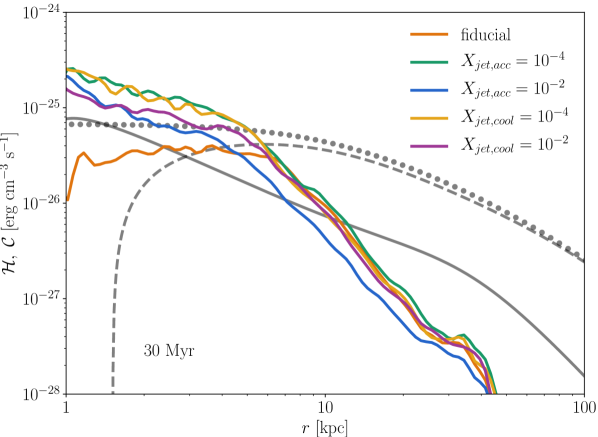
Figure 20: Same as in Fig. 8, here showing profiles of lower resolution simulations with varying jet tracer thresholds for subgrid CR acceleration $X_{\mathrm{jet,acc}}$ and CR Alfvén cooling $X_{\mathrm{jet,cool}}$ at $30\ \mathrm{Myr}$. Varying the thresholds by an order of magnitude in both directions, the resulting heating rate differs at most by a factor of a few at small radii and converges at large radii.

To remain consistent with our definition of the lobe, i.e., $X_{\mathrm{jet}}<10^{-3}$, we set the jet tracer threshold for CR acceleration and cooling to $X_{\mathrm{jet,acc}}=X_{\mathrm{jet,cool}}=10^{-3}$. To test the robustness of our choice, Fig. 20 shows radial profiles of the CR-induced Alfvén wave heating rate if we vary $X_{\mathrm{jet,acc}}$ and $X_{\mathrm{jet,cool}}$ each by one order of magnitude. In the inner 10 kpc, the CR distributions agree within a factor of a few. Further out in the vicinity of the bubbles, the radial profiles agree well. We generally find that changing the cooling threshold $X_{\mathrm{jet,cool}}$ has a smaller impact than varying the acceleration threshold $X_{\mathrm{jet,acc}}$.

References

- Anjiri et al. (2014) Anjiri M., Mignone A., Bodo G., Rossi P., 2014, MNRAS, 442, 2228
- Asai et al. (2007) Asai N., Fukuda N., Matsumoto R., 2007, ApJ, 663, 816
- Bambic et al. (2018) Bambic C. J., Morsony B. J., Reynolds C. S., 2018, preprint (arXiv:1801.06233)
- Bîrzan et al. (2004) Bîrzan L., Rafferty D. A., McNamara B. R., Wise M. W., Nulsen P. E. J., 2004, ApJ, 607, 800
- Bîrzan et al. (2008) Bîrzan L., McNamara B. R., Nulsen P. E. J., Carilli C. L., Wise M. W., 2008, ApJ, 686, 859
- Bonafede et al. (2010) Bonafede A., Feretti L., Murgia M., Govoni F., Giovannini G., Dallacasa D., Dolag K., Taylor G. B., 2010, A&A, 513, A30
- Bourne & Sijacki (2017) Bourne M. A., Sijacki D., 2017, MNRAS, 472, 4707
- Brüggen & Kaiser (2001) Brüggen M., Kaiser C. R., 2001, MNRAS, 325, 676
- Brüggen & Kaiser (2002) Brüggen M., Kaiser C. R., 2002, Nature, 418, 301
- Brüggen et al. (2002) Brüggen M., Kaiser C. R., Churazov E., Enßlin T. A., 2002, MNRAS, 331, 545
- Churazov et al. (2001) Churazov E., Brüggen M., Kaiser C. R., Böhringer H., Forman W., 2001, ApJ, 554, 261
- Churazov et al. (2003) Churazov E., Forman W., Jones C., Böhringer H., 2003, ApJ, 590, 225
- Cielo et al. (2018) Cielo S., Babul A., Antonuccio-Delogu V., Silk J., Volonteri M., 2018, preprint (arXiv:1801.04276)
- Croston & Hardcastle (2014) Croston J. H., Hardcastle M. J., 2014, MNRAS, 438, 3310
- Croston et al. (2008) Croston J. H., Hardcastle M. J., Birkinshaw M., Worrall D. M., Laing R. A., 2008, MNRAS, 386, 1709
- Croston et al. (2018) Croston J. H., Ineson J., Hardcastle M. J., 2018, MNRAS, 476, 1614
- Duran et al. (2016) Duran R. B., Tchekhovskoy A., Giannios D., 2016, MNRAS, 469, 4957
- Dursi (2007) Dursi L. J., 2007, ApJ, 670, 221
- Dursi & Pfrommer (2008) Dursi L. J., Pfrommer C., 2008, ApJ, 677, 993
- Enßlin & Brüggen (2002) Enßlin T. A., Brüggen M., 2002, MNRAS, 331, 1011
- Fabian (2012) Fabian A. C., 2012, ARA&A, 50, 455
- Fabian et al. (2000) Fabian A. C., et al., 2000, MNRAS, 318, L65
- Fabian et al. (2003) Fabian A. C., Sanders J. S., Allen S. W., Crawford C. S., Iwasawa K., Johnstone R. M., Schmidt R., Taylor G. B., 2003, MNRAS, 344, L43
- Fabian et al. (2011) Fabian A. C., et al., 2011, MNRAS, 418, 2154
- Fabian et al. (2017) Fabian A. C., Walker S. A., Russell H. R., Pinto C., Sanders J. S., Reynolds C. S., 2017, MNRAS, 464, L1
- Fanaroff & Riley (1974) Fanaroff B. L., Riley J. M., 1974, MNRAS, 167, 31P
- Guo & Mathews (2011) Guo F., Mathews W. G., 2011, ApJ, 728, 9
- Guo & Oh (2008) Guo F., Oh S. P., 2008, MNRAS, 384, 251
- Heesen et al. (2018) Heesen V., et al., 2018, MNRAS, 474, 5049
- Heinz et al. (2006) Heinz S., Brüggen M., Young A., Levesque E., 2006, MNRASL, 373, 65
- Hillel & Soker (2016) Hillel S., Soker N., 2016, MNRAS, 455, 2139
- Hitomi Collaboration et al. (2016) Hitomi Collaboration et al., 2016, Nature, 535, 117
- Jacob & Pfrommer (2017a) Jacob S., Pfrommer C., 2017a, MNRAS, 467, 1449
- Jacob & Pfrommer (2017b) Jacob S., Pfrommer C., 2017b, MNRAS, 467, 1478
- Jones & De Young (2005) Jones T. W., De Young D. S., 2005, ApJ, 624, 586
- Kannan et al. (2017) Kannan R., Vogelsberger M., Pfrommer C., Weinberger R., Springel V., Hernquist L., Puchwein E., Pakmor R., 2017, The Astrophysical Journal Letters, 837, L18
- Kim & Narayan (2003) Kim W.-T., Narayan R., 2003, ApJ, 596, 889
- Kuchar & Enßlin (2011) Kuchar P., Enßlin T. A., 2011, A&A, 529, 13
- Kulsrud (2005) Kulsrud R. M., 2005, Plasma Physics for Astrophysics. Princeton University Press, Princeton, NJ
- Kulsrud & Pearce (1969) Kulsrud R., Pearce W. P., 1969, ApJ, 156, 445
- Laing & Bridle (2013) Laing R. A., Bridle A. H., 2013, MNRAS, 432, 1114
- Laing & Bridle (2014) Laing R. A., Bridle A. H., 2014, MNRAS, 437, 3405
- Leccardi & Molendi (2008) Leccardi A., Molendi S., 2008, A&A, 486, 359
- Li et al. (2017) Li Y., Ruszkowski M., Bryan G. L., 2017, ApJ, 847, 106
- Lind et al. (1989) Lind K. R., Payne D. G., Meier D. L., Roger D. B., 1989, ApJ, 344, 89
- Loewenstein et al. (1991) Loewenstein M., Zweibel E. G., Begelman M. C., 1991, ApJ, 377, 392
- Lyutikov (2006) Lyutikov M., 2006, MNRAS, 373, 73
- Martizzi & Quataert (2018) Martizzi D., Quataert E., 2018, preprint (arXiv:1805.06461)
- Massaglia et al. (2016) Massaglia S., Bodo G., Rossi P., Capetti S., Mignone A., 2016, A&A, 596, A12
- McNamara & Nulsen (2007) McNamara B. R., Nulsen P. E. J., 2007, ARA&A, 45, 117
- McNamara & Nulsen (2012) McNamara B. R., Nulsen P. E. J., 2012, New J. Phys., 14, 40
- Mendygral et al. (2012) Mendygral P. J., Jones T. W., Dolag K., 2012, ApJ, 750, 17pp
- Morganti et al. (1988) Morganti R., Fanti R., Gioia I. M., Harris D. E., Parma P., de Ruiter H., 1988, A&A, 189, 11
- Morsony et al. (2010) Morsony B. J., Heinz S., Brüggen M., Ruszkowski M., 2010, MNRAS, 407, 1277
- Mukherjee et al. (2016) Mukherjee D., Bicknell G. V., Sutherland R., Wagner A., 2016, MNRAS, 461, 967
- Navarro et al. (1996) Navarro J. F., Frenk C. S., White S. D. M., 1996, ApJ, 462, 563
- Navarro et al. (1997) Navarro J. F., Frenk C. S., White S. D. M., 1997, ApJ, 490, 493
- O’Neill & Jones (2010) O’Neill S. M., Jones T. W., 2010, ApJ, 710, 180
- O’Neill et al. (2009) O’Neill S. M., De Young D. S., Jones T. W., 2009, ApJ, 694, 1317
- Ogiya et al. (2018) Ogiya G., Biernacki P., Hahn O., Teyssier R., 2018, preprint (arXiv:1802.02177)
- Pakmor & Springel (2013) Pakmor R., Springel V., 2013, MNRAS, 432, 176
- Pakmor et al. (2011) Pakmor R., Bauer A., Springel V., 2011, MNRAS, 418, 1392
- Pakmor et al. (2016a) Pakmor R., Springel V., Bauer A., Mocz P., Munoz D. J., Ohlmann S. T., Schaal K., Zhu C., 2016a, MNRAS, 455, 1134
- Pakmor et al. (2016b) Pakmor R., Pfrommer C., Simpson C. M., Kannan R., Springel V., 2016b, MNRAS, 462, 2603
- Perucho & Martí (2007) Perucho M., Martí J. M., 2007, MNRAS, 382, 526
- Perucho et al. (2010) Perucho M., Martí J. M., Cela J. M., Hanasz M., Cruz R. D., Rubio F., 2010, A&A, 519, A41
- Perucho et al. (2017) Perucho M., Martí J. M., Quilis V., Borja-Lloret M., 2017, MNRAS, 471, L120
- Peterson & Fabian (2006) Peterson J. R., Fabian A. C., 2006, Phys. Rep., 427, 1
- Pfrommer (2013) Pfrommer C., 2013, ApJ, 779, 10
- Pfrommer & Dursi (2010) Pfrommer C., Dursi J., 2010, Nat. Phys., 6, 520
- Pfrommer et al. (2017) Pfrommer C., Pakmor R., Schaal K., Simpson C. M., Springel V., 2017, MNRAS, 465, 4500
- Powell et al. (1999) Powell K. G., Roe P. L., Linde T. J., Gombosi T. I., De Zeeuw D. L., 1999, Journal of Computational Physics, 154, 284
- Quataert (2008) Quataert E., 2008, ApJ, 673, 758
- Reynolds et al. (2001) Reynolds C. S., Heinz S., Begelman M. C., 2001, ApJ, 549, 179
- Reynolds et al. (2002) Reynolds C. S., Heinz S., Begelman M. C., 2002, MNRAS, 332, 271
- Reynolds et al. (2005) Reynolds C. S., McKernan B., Fabian A. C., Stone J. M., Vernaleo J. C., 2005, MNRAS, 357, 242
- Reynolds et al. (2015) Reynolds C. S., Balbus S. A., Schekochihin A. A., 2015, ApJ, 815, 41
- Ruszkowski et al. (2007) Ruszkowski M., Enßlin T. A., Brüggen M., Heinz S., Pfrommer C., 2007, MNRAS, 378, 662
- Ruszkowski et al. (2008) Ruszkowski M., Enßlin T. A., Brüggen M., Begelman M. C., Churazov E., 2008, MNRAS, 383, 1359
- Ruszkowski et al. (2017) Ruszkowski M., Yang H. Y. K., Reynolds C. S., 2017, ApJ, 844, 13
- Sanders & Fabian (2008) Sanders J. S., Fabian A. C., 2008, MNRASL, 390, L93
- Schaal & Springel (2015) Schaal K., Springel V., 2015, MNRAS, 446, 3992
- Sharma et al. (2009) Sharma P., Chandran B. D. G., Quataert E., Parrish I. J., 2009, ApJ, 699, 348
- Sijacki & Springel (2006) Sijacki D., Springel V., 2006, MNRAS, 371, 1025
- Sijacki et al. (2008) Sijacki D., Pfrommer C., Springel V., Enßlin T. A., 2008, MNRAS, 387, 1403
- Soker (2003) Soker N., 2003, MNRAS, 342, 463
- Springel (2010) Springel V., 2010, MNRAS, 401, 791
- Sternberg & Soker (2008) Sternberg A., Soker N., 2008, MNRASL, 389, 13
- Tchekhovskoy & Bromberg (2016) Tchekhovskoy A., Bromberg O., 2016, MNRAS, 461, L46
- Turner (2018) Turner R. J., 2018, MNRAS, 476, 2522
- Vantyghem et al. (2014) Vantyghem A. N., McNamara B. R., Russell H. R., Main R. A., Nulsen P. E. J., Wise M. W., Hoekstra H., Gitti M., 2014, MNRAS, 442, 3192
- Vikhlinin et al. (2001) Vikhlinin A., Markevitch M., Murray S. S., 2001, ApJ, 551, 160
- Weinberger et al. (2017) Weinberger R., Ehlert K., Pfrommer C., Pakmor R., Springel V., 2017, MNRAS, 470, 4530
- Wentzel (1971) Wentzel G. W., 1971, ApJ, 163, 503
- Wiener et al. (2013) Wiener J., Oh S. P., Guo F., 2013, MNRAS, 434, 2209
- Wiener et al. (2017) Wiener J., Pfrommer C., Oh S. P., 2017, MNRAS, 467, 906
- Worrall (2009) Worrall D. M., 2009, Astronomy and Astrophysics Review, 17, 1
- Wykes et al. (2015) Wykes S., Hardcastle M. J., Karakas A. I., Vink J. S., 2015, MNRAS, 447, 1001
- Yang et al. (2016) Yang H.-Y. K., Reynolds C. S., Yang H.-Y. K., Reynolds C. S., 2016, ApJ, 818, 181
- Zweibel (2013) Zweibel E. G., 2013, Phys. Plasmas, 20, 055501