Instability of Supersonic Cold Streams Feeding Galaxies III: Kelvin-Helmholtz Instability in Three Dimensions

Abstract

We study the effects of Kelvin-Helmholtz instability (KHI) on the cold streams that feed high-redshift galaxies through their hot haloes, generalizing our earlier analyses of a 2D slab to a 3D cylinder, but still limiting our analysis to the adiabatic case with no gravity. We combine analytic modeling and numerical simulations in the linear and non-linear regimes. For subsonic or transonic streams with respect to the halo sound speed, the instability in 3D is qualitatively similar to 2D, but progresses at a faster pace. For supersonic streams, the instability grows much faster in 3D and can be qualitatively different due to azimuthal modes, which introduce a strong dependence on the initial width of the stream-background interface. Using analytic toy models and approximations supported by high-resolution simulations, we apply our idealized hydrodynamical analysis to the astrophysical scenario. The upper limit for the radius of a stream that disintegrates prior to reaching the central galaxy is $\sim 70\%$ larger than the 2D estimate; it is in the range $0.5-5\%$ of the halo virial radius, decreasing with increasing stream density and velocity. Stream disruption generates a turbulent mixing zone around the stream with velocities at the level of $\sim 20\%$ of the initial stream velocity. KHI can cause significant stream deceleration and energy dissipation in 3d, contrary to 2D estimates. For typical streams, up to $10-50\%$ of the gravitational energy gained by inflow down the dark-matter halo potential can be dissipated, capable of powering Lyman-alpha blobs if most of it is dissipated into radiation.

1 Introduction

Dark matter haloes with virial masses $M_{\rm v}\lower 2.58333pt\hbox{$\;\buildrel>\over{\sim}\;$}10^{12}{\rm M}_{\odot}$ are predicted to contain hot gas at the virial temperature, $T_{\rm v}\lower 2.58333pt\hbox{$\;\buildrel>\over{\sim}\;$}10^{6}\,{\rm K}$, with cooling times exceeding the Hubble time (Rees & Ostriker, 1977; White & Rees, 1978; Birnboim & Dekel, 2003; Dekel & Birnboim, 2006; Fielding et al., 2017). However, during the peak phase of star- and galaxy-formation at redshifts $z=1-4$, massive galaxies of $\sim 10^{11}{\rm M}_{\odot}$ in baryons, which are predicted to reside in such haloes, exhibit star-formation rates (SFRs) of order $100\,M_{\odot}\,{\rm yr}^{-1}$ (Genzel et al., 2006; Förster Schreiber et al., 2006; Elmegreen et al., 2007; Genzel et al., 2008; Stark et al., 2008), only a factor of $\sim 2$ below the theoretical cosmological gas accretion rate (Dekel et al., 2009, 2013). This implies that accreted gas must efficiently cool, or never be heated, and penetrate down to the central galaxy.

According to the developing theoretical picture of galaxy formation, these massive galaxies reside at the nodes of the cosmic web, and are penetrated by cosmic filaments of dark matter (Bond, Kofman & Pogosyan, 1996; Springel et al., 2005). Gas flowing along these filaments is significantly denser than the halo gas, allowing it to cool rapidly (Dekel & Birnboim, 2006). These “cold streams” are expected to penetrate through the hot circumgalactic medium (CGM) onto the central galaxy while retaining a temperature of $T_{\rm s}\lower 2.58333pt\hbox{$\;\buildrel>\over{\sim}\;$}10^{4}\,{\rm K}$, set by the drop in the cooling rate below this temperature (Sutherland & Dopita, 1993), and by photo-heating by the UV background, though the interiors of streams are expected to be at least partly self-shielded (Goerdt et al., 2010; Faucher-Giguère et al., 2010).

The above theoretical picture is supported by cosmological simulations (Kereš et al., 2005; Ocvirk, Pichon & Teyssier, 2008; Dekel et al., 2009; Ceverino, Dekel & Bournaud, 2010; Faucher-Giguère, Kereš & Ma, 2011; van de Voort et al., 2011), which show cold streams with diameters of a few to ten percent of the halo virial radius penetrating deep into the haloes of massive star-forming galaxies (SFGs). These streams supply gas to the haloes at rates of $\sim 100\,M_{\odot}\,{\rm yr}^{-1}$, comparable to both the theoretical cosmological gas accretion rate and the observed SFR in SFGs. This implies that cold streams must carry a significant fracton of the cosmological gas accretion rate onto the central galaxy (Dekel et al., 2009, 2013).

In cosmological simulations, the streams maintain roughly constant inflow velocities as they travel from the outer halo to the central galaxy (Dekel et al., 2009; Goerdt & Ceverino, 2015), rather than accelerating in the halo gravitational potential. This indicates that a dissipation process acts upon the streams in the CGM, though its source is yet to be identified. As the cold streams are likely dense enough to be self-shielded from the UV background (Goerdt et al., 2010; Faucher-Giguère et al., 2010), they consist mostly of neutral Hydrogen and the associated energy loss may be observed as Lyman-$\alpha$ emission (Dijkstra & Loeb, 2009; Goerdt et al., 2010; Faucher-Giguère et al., 2010), possibly accounting for observed Lyman-$\alpha$ “blobs” at $z>2$ (Steidel et al., 2000; Matsuda et al., 2006, 2011). Recent observations have revealed massive extended cold components in the CGM of high-redshift galaxies, whose spatial and kinematic properties are consistent with predictions for cold streams (Cantalupo et al., 2014; Martin et al., 2014a, b; Borisova et al., 2016; Fumagalli et al., 2017; Leclercq et al., 2017; Arrigoni Battaia et al., 2018).The cold streams may also be visible in Lyman-$\alpha$ absorption, possibly accounting for several observed systems (Fumagalli et al., 2011; Goerdt et al., 2012; van de Voort et al., 2012; Bouché et al., 2013, 2016; Prochaska, Lau & Hennawi, 2014).

While there is growing evidence that cold streams play an important role in galaxy formation at high redshift, their evolution in the CGM is still a matter of debate. In particular, it remains unclear whether the streams indeed penetrate all the way to the central galaxy or whether they dissolve or fragment along the way, what fraction of their energy is dissipated in the halo and whether this dissipation is observable, and what the net effect of all this is on the gas that eventually joins the galaxy. Cosmological simulations used to study these issues typically reach a resolution of one hundred to a few hundred pc within streams in the outer halo, comparable to the stream width. Hydrodynamic and other instabilities at smaller scales are thus not captured properly, rendering current cosmological simulations ill-suited to investigate the detailed evolution of cold streams. This may be the cause of apparent contradictions between properties of cold streams predicted by different simulations. For example, simulations using the moving mesh code AREPO (Springel, 2010; Vogelsberger et al., 2012) suggest that streams heat up and dissolve at $\lower 2.58333pt\hbox{$\;\buildrel>\over{\sim}\;$}0.5R_{\rm v}$ (Nelson et al., 2013), contrary to comparable Eulerian AMR (Ceverino, Dekel & Bournaud, 2010; Danovich et al., 2015) and Lagrangian SPH (Kereš et al., 2005; Faucher-Giguère et al., 2010) simulations, where the streams remain cold and collimated outside of an interaction region at $\sim 0.25R_{\rm v}$. The interpretation of these results is uncertain due to insufficient resolution (see also Nelson et al., 2016), motivating a more careful study of cold stream evolution in the CGM.

As an alternative to cosmological simulations, in this series of papers we use analytic models and idealized simulations, progressively increasing the complexity of our analysis. In two previous papers, Mandelker et al. (2016), hereafter M16, and Padnos et al. (2018), hereafter P18, we studied the effects of Kelvin-Helmholtz Instability (KHI) on the evolution of cold streams. We found that for a reasonable range of stream density, velocity and radius, KHI was expected to become highly nonlinear within a virial crossing time, with the number of e-foldings of growth experienced by a linear perturbation ranging from $\sim 0.1-100$ (M16). A detailed analysis of the nonlinear evolution of KHI in two dimensions revealed that sufficiently narrow streams should dissintegrate in the CGM prior to reaching the central galaxy (P18). The condition for breakup ranged from $R_{\rm s}\lower 2.58333pt\hbox{$\;\buildrel<\over{\sim}\;$}0.003R_{\rm v}$ to $R_{\rm s}\lower 2.58333pt\hbox{$\;\buildrel<\over{\sim}\;$}0.03R_{\rm v}$, where $R_{\rm s}$ is the stream radius and $R_{\rm v}$ is the halo virial radius, with denser, faster streams having smaller critical radii for disintegration. However, due to the large stream inertia, KHI was found to have only a small effect on the stream inflow rate and a small contribution to heating and subsequent Lyman-$\alpha$ cooling emission.

In this paper, we extend the study of the nonlinear evolution of KHI in cold streams to three dimensional cylinders, using both analytic models and numerical simulations. As described in detail in §2, the two dimensional analysis presented in P18 is limited in a number of ways, both quantitative and qualitative. Indeed, KHI is known to evolve more rapidly and more violently in three dimensions (Bassett & Woodward, 1995; Bodo et al., 1998; Xu, Hardee & Stone, 2000), thus motivating our current analysis.

While several previous works have used numerical simulations to study the nonlinear evolution of KHI in cylindrical geometry (e.g. Hardee, Clarke & Howell, 1995; Bassett & Woodward, 1995; Bodo et al., 1998; Freund, Lele & Moin, 2000; Bogey, Marsden & Bailly, 2011), almost all of them focussed on light or equidense jets, with $\delta=\rho_{\rm s}/\rho_{\rm b}\leq 1$, and none of them explored the regime $\delta>10$, relevant for cosmic cold streams. Furthermore, many of these studies focussed on spatial, rather than temporal stability analysis (see §2), and are thus not precisely equivalent to our study. A notable exception is Bodo et al. (1998) who studied the temporal stability of a 3d cylindrical jet with $\delta=10$ and compared it to that of a 2d slab. However, only one such simulation was presented and no attempt was made to estimate how properties such as stream deceleration or disruption might scale with Mach number or density contrast. Furthermore, the resolution in our simulations is much higher than those of Bodo et al. (1998), reaching up to 5 times as many grid cells per stream diameter. Our work offers the first comprehensive study of temporal nonlinear growth of KHI in dense cylindrical streams, and the first to focus on deceleration due to KHI in these systems, providing estimates for the relevant timescales as a function of Mach number and density contrast.

The remainder of this paper is organized as follows. In §2 we summarize the theoretical understanding of the evolution of KHI in the linear and nonlinear regimes, in 2d and in 3d. In §3 we discuss the numerical simulations used to study KHI in 3d cylinders and the techniques used for their analysis. In §4 we present the results of our numerical analysis and compare these to our analytic predictions. In §5 we apply the results of our idealized models to the astrophysical scenario of cold streams in hot halos. We obtain estimates of the potential fragmentation, reduction of inflow rates, and Lyman-$\alpha$ emission due to KHI in cold streams. Readers only interested in the astrophysical implications of our analysis rather than the detailed hydrodynamics can skip directly to this section without loss of clarity. In §6 we discuss the potential effects of additional physics not included in our current analysis, and outline future work. We summarize our conclusions in §7.

2 Analytic Theory

In this section, we review the linear theory of KHI in 2d slabs and 3d cylinders, and the nonlinear growth of KHI in 2d slabs. We limit this discussion to the elements necessary for understanding our current analysis, and refer interested readers to M16 and P18 for further details and additional references. We then discuss our expectations for the nonlinear behaviour of KHI in 3d cylinders, which will be tested with simulations in §4.

2.1 Linear Analysis

We consider the case of a cold, dense stream confined in a hot, dilute background, with no radiative cooling or gravity. The fluids are characterized by their respective densities and speeds of sound, $\rho_{\rm b,s}$ and $c_{\rm b,s}$, and are assumed to have an ideal gas equation of state with adiabatic index $\gamma=5/3$. We assume that the fluids are in pressure equilibrium. We adopt a reference frame where the background is initially stationary, $V_{\rm b}=0$, while the stream has velocity $V_{\rm s}=V$ parallel to the stream-background interface. The instability is dominated by two dimensionless parameters: the density contrast, $\delta\equiv\rho_{\rm s}/\rho_{\rm b}$, and the Mach number with respect to the background speed of sound, $M_{\rm b}\equiv V/c_{\rm b}$. Due to pressure equilibrium, the temperatures and speeds of sound satisfy $T_{\rm b}/T_{\rm s}=\delta$ and $c_{\rm b}/c_{\rm s}=\delta^{1/2}$. The Mach number with respect to the stream speed of sound satisfies $M_{\rm s}\equiv V/c_{\rm s}=\delta^{1/2}M_{\rm b}$.

We limit our discussion to temporal stability analysis, finding the growth rates, $\omega_{\rm I}$, as a function of wavenumber, $k=2\pi/\lambda$, for all unstable eigenmodes of the system. In the linear regime, unstable eigenmodes grow exponentially with time as $\propto{\rm exp}(t/t_{\rm KH})$, where $t_{\rm KH}=\omega_{\rm I}^{-1}$ is the Kelvin-Helmholtz time of the associated eigenmode.

The simplest variant of the problem is a planar sheet, where two semi-infinite fluids are initially separated by a single planar interface at $x=0$. The planar sheet admits unstable eigenmodes that spatially decay exponentially away from the initial interface and are therefore called surface modes. Instability occurs if and only if the Mach number is below a critical value,

$$M_{\rm b}<M_{\rm crit}=\left(1+\delta^{-1/3}\right)^{3/2}.$$ (1)

If eq. (1) is satisfied, perturbations at all wavelength are unstable with $t_{\rm KH}\propto\lambda/V$, while the proportionality constant depends on $M_{\rm b}$ and $\delta$ (M16).

Two additional, more complicated, variants of the problem are a planar slab, where the stream fluid is initially confined to a slab of finite thickness, $-R_{\rm s}<x<R_{\rm s}$, surrounded by the background fluid, and a cylindrical stream, where the stream fluid is initially confined to a cylinder of finite radius, $r<R_{\rm s}$, surrounded by the background fluid. Both of these also admit surface mode solutions, which converge to the same dispersion relation as in the planar sheet in the incompressible ($M_{\rm b}\ll 1$), short wavelength ($\lambda\lower 2.58333pt\hbox{$\;\buildrel<\over{\sim}\;$}R_{\rm s}$) limit. Each unstable mode is characterized by a symmetry-order, $m$. $m=0$ corresponds to axisymmetric perturbations, called pinch-modes or P-modes. $m=1$ corresponds to antisymmetric perturbations, called sinusoidal-modes or S-modes in the slab, and helical-modes in the cylinder. In slab geometry, these are the only two symmetry modes. However, a cylinder admits infinitely many symmetry modes, collectively referred to as fluting-modes. These have $m=2,3,...$ corresponding to the number of azimuthal nodes on the circumference of the cylinder, and azimuthal wavelengths $\lambda_{\varphi}=2\pi R_{\rm s}/m$.

When $M_{\rm b}>M_{\rm crit}$, surface modes stabilize. However, another class of unstable solutions, called body modes, are excited. These are associated with waves reverberating between the stream boundaries, forming a pattern of nodes inside the stream that resembles standing waves propagating through a waveguide. Body modes are unstable if and only if

$$M_{\rm tot}\equiv\frac{V}{c_{\rm s}+c_{\rm b}}=\frac{\sqrt{\delta}}{1+\sqrt{\delta}}M_{\rm b}>1,$$ (2)

which is roughly the opposite of eq. (1). The system is therefore always unstable, with the $(M_{\rm b},\delta)$ parameter space divided into a surface-mode-dominated region and a body-mode-dominated region, and a narrow range of parameters allowing coexistence (M16).

At shorter and shorter wavelengths, an ever-increasing number of unstable body modes appear, characterized by the number of transverse nodes in the perturbed variables within the stream. These form a discrete set with different frequencies, $\{\omega_{\rm m,n}(k)\}$. For each symmetry-oder $m$, the $n=0$ mode is called the fundamental $m$ mode, while modes with $n\geq 1$ are referred to as reflected modes. The effective Kelvin-Helmholtz time at a given wavelength is determined by the mode with the largest growth rate at that wavelength, the fastest growing mode. At short wavelengths, $t_{\rm KH}\sim t_{\rm sc}/{\rm ln}(\beta R_{\rm s}/\lambda)$, with $t_{\rm sc}=2R_{\rm s}/c_{\rm s}$ the stream sound crossing time, and $\beta$ a function of $M_{\rm b}$ and $\delta$ (M16). While shorter wavelength perturbations have larger growth rates for both surface and body modes, the dependence on $\lambda$ is weaker for body modes, logarithmic rather than linear. In general, the growth rates of body modes are smaller than those of surface modes, while for both surface and body modes the instability is attenuated as either the Mach number or the density contrast are increased.

2.2 Nonlinear Evolution of Surface Modes

2.2.1 Surface Modes at $M_{\rm b}<M_{\rm crit}$

We begin by considering 2d slab geometry. Each interface of a slab behaves as a vortex sheet, with the vorticity perpendicular to the plane. The nonlinear behaviour is dominated by vortex mergers, resulting in self-similar growth of the shear layer separating the fluids. The width of the shear layer, $h$, evolves as

$$\frac{h}{R_{\rm s}}=\frac{\alpha Vt}{R_{\rm s}}=\frac{\alpha t}{t_{\rm s}},$$ (3)

where $t_{\rm s}=R_{\rm s}/V$ is the characteristic time for surface mode evolution, and $\alpha$ is a dimensionless growth rate that depends primarily on $M_{\rm tot}$, and is typically in the range $\alpha\sim 0.05-0.25$. This behaviour is independent of the initial perturbations. An empirical fit to $\alpha$ was proposed by Dimotakis (1991),

$$\alpha\simeq 0.21\times\left[0.8{\rm exp}\left(-3M_{\rm tot}^{2}\right)+0.2\right].$$ (4)

The centres of the largest eddies in the shear layer, with sizes of order the shear layer thickness $h$, move downstream at the convection velocity,

$$V_{\rm c}=\frac{\sqrt{\delta}}{1+\sqrt{\delta}}V,$$ (5)

which can be derived by assuming that in between each pair of eddies there is a stagnation point, where the ram pressure from both fluids must be equal (Coles, 1985; Dimotakis, 1986). In 2d slabs this corresponds to the center of mass velocity in the shear layer (P18). Combining this result with conservation of mass and momentum of material entering the shear layer as it expands yields the entrainment ratio, the ratio of shear layer penetration into the stream to penetration into the background (P18),

$$E_{\rm v}\equiv\frac{h_{\rm s}}{h_{\rm b}}=\delta^{-1/2}.$$ (6)

Combining eqs. (3) and (6) with $h=h_{\rm s}+h_{\rm b}$ yields

$$\frac{h_{\rm s}}{R_{\rm s}}=\frac{1}{1+\sqrt{\delta}}\frac{\alpha t}{t_{\rm s}},$$ (7)

$$\frac{h_{\rm b}}{R_{\rm s}}=\frac{\sqrt{\delta}}{1+\sqrt{\delta}}\frac{\alpha t}{t_{\rm s}},$$ (8)

Stream disruption occurs when $h_{\rm s}=R_{\rm s}$ so the shear layer encompasses the entire stream. This occurs at time (P18)

$$t_{\rm dis,\,surface}=\frac{1+\sqrt{\delta}}{\alpha}t_{\rm s}.$$ (9)

As the shear layer expands into the background, the initial momentum of the stream is distributed over more and more material. The deceleration of the stream thus occurs over a characteristic timescale (P18)

$$\tau_{\rm surface,\,2d}=\frac{\delta+\sqrt{\delta}}{\alpha}t_{\rm s}=\sqrt{\delta}~{}t_{\rm dis,\,surface}.$$ (10)

This marks the time when the amount of background mass swept up by the shear layer is equal to the initial stream mass, and thus corresponds to the time when the stream velocity is reduced to half its initial value. This is longer than the disruption timescale for any $\delta>1$.

To develop an analogous description of the nonlinear evolution of surface modes in 3d cylinders, we model the cylindrical interface between the stream and the background as a vortex ring, where the vorticity is concentrated entirely in the azimuthal direction. This is supported by simulations as discussed in §4.1. In this model, the fluid motion on large scales remains confined to the $z-r$ plane at each azimuthal angle $\varphi$. This implies that any cross-section through the stream along its axis (at a constant $\varphi$) will appear identical to a planar slab, growing by vortex mergers in the $z-r$ plane. We thus predict that eqs. (3)-(9) will hold for shear layers in cylindrical streams as well.

A qualitative difference between shear layer growth in 2d and 3d arrises due to the nature of the energy cascade. In 2d, there is only an inverse cascade to larger scales, so the largest eddies remain coherent and grow larger as they merge, with $\alpha$ roughly constant throughout the evolution. In 3d, the inverse cascade coexists with a direct cascade to smaller scales which breaks up large eddies, generates turbulence, and enhances mixing. This may cause the shear layer growth rate to decline, as energy is transferred from the largest scales which drive the growth to small scales which drive turbulence and generate heat through dissipation.

Deceleration is expected to occur faster in 3d cylinders than in 2d slabs, because the shear layer will sweep up mass at a higher rate as it expands into the background. The penetration depth of the shear layer into the background when it has swept up a mass equal to the initial stream mass is given by

$$\rho_{\rm b}\pi[(R_{\rm s}+h_{\rm b})^{2}-R_{\rm s}^{2}]L=\rho_{\rm s}\pi R_{\rm s}^{2}L.$$ (11)

Combined with eq. (8) this yields the expected deceleration timescale for a 3d cylinder,

$$\begin{array}[]{c}\tau_{\rm surface,\,3d}=\dfrac{\left(1+\sqrt{\delta}\right)\left(\sqrt{1+\delta}-1\right)}{\alpha\sqrt{\delta}}t_{\rm s}\\ =\dfrac{\sqrt{1+\delta}-1}{\delta}\tau_{\rm surface,\,2d}.\end{array}$$ (12)

For $\delta=1$, $10$, and $100$, we have $\tau_{\rm surface,\,3d}/\tau_{\rm surface,\,2d}\simeq 0.41$, $0.23$, and $0.09$ respectively. Furthermore, while for 2d slabs the deceleration timescale is always longer than the disruption timescale, for 3d cylinders we have $\tau_{\rm surface,\,3d}/t_{\rm dis,\,surface}\simeq 0.41$, $0.73$ and $0.91$ for $\delta=1$, $10$, and $100$. Stream deceleration is thus predicted to be much more significant in 3d cylinders than 2d slabs.

2.2.2 Surface Modes at $M_{\rm b}>M_{\rm crit}$

The largest qualitative difference between 2d and 3d systems is that the strict separation between a surface-mode- and a body-mode-dominated regime is an accurate description only in 2d. In 3d, unstable surface-modes exist at $M_{\rm b}>M_{\rm crit}$ as well, associated with large values of the azimuthal wave number, $m$. This is because the Mach number determining surface mode stability in eq. (1) corresponds to the velocity component parallel to the perturbation wave-vector, $V_{\rm k}=\vec{V}\cdot\hat{k}$ (M16). In 2d systems, $V_{\rm k}=V$ by definition. However, in cylindrical geometry, modes with $m>1$ have components in the $\hat{\varphi}$ direction, while the velocity is in the $\hat{z}$ direction. As a result, the effective Mach number associated with an azimuthal mode number $m$ is reduced by a factor $[1+(m/K)^{2}]^{-1/2}$, where $K=kR_{\rm s}$, and surface modes are unstable for

$$m>m_{\rm crit}=K[(M_{\rm b}/M_{\rm crit})^{2}-1]^{1/2}.$$ (13)

For example, for wavelengths $\lambda\sim 2R_{\rm s}$ and $M_{\rm b}\sim 1.5M_{\rm crit}$ (reasonable for cold streams), eq. (13) predicts that surface modes will be unstable for $m\lower 2.58333pt\hbox{$\;\buildrel>\over{\sim}\;$}4$. Note that $m_{\rm crit}$ depends on both $M_{\rm b}$ and $\delta$ through $M_{\rm crit}$, as well as on $\lambda/R_{\rm s}$ through $K$, making the overall behaviour very complicated. Regardless of the value of $m$, we expect unstable surface modes to behave according to the description in §2.2.1.

Table 1: Critical wavelengths and corresponding linear growth rates for stream disruption due to body modes, for the $(M_{\rm b},\delta)$ parameters presented in this §4.2. The columns show, from left to right, the Mach number of the stream with respect to the background sound speed, $M_{\rm b}$, the density contrast between the stream and the background, $\delta$, the critical wavelength for stream disruption due to body modes in units of the stream radius, $\lambda_{\rm crit}/R_{\rm s}$, for 2d slabs and 3d cylinders, and the corresponding linear growth times in units of the sound crossing time, $t_{\rm KH}/t_{\rm sc}$, for 2d slabs and 3d cylinders. This growth time can be used in eq. (16) to estimate the time for stream disruption due to body modes. For 2d slabs we have $t_{\rm KH}\sim t_{\rm sc}$ while for 3d cylinders we have $t_{\rm KH}\sim 0.5t_{\rm sc}$

$M_{\rm b}$	$\delta$	$\lambda_{\rm crit,2d}/R_{\rm s}$	$\lambda_{\rm crit,3d}/R_{\rm s}$	$t_{\rm KH,2d}/t_{\rm sc}$	$t_{\rm KH,3d}/t_{\rm sc}$
5.0	1	17	13	1.17	0.75
2.5	5	14	9	0.91	0.55
2.0	10	11	8.5	0.86	0.54
2.5	20	12	11	0.93	0.53
2.0	100	13	11	0.86	0.51

2.3 Nonlinear Evolution of Body Modes

Nonlinear evolution of body modes occurs through global deformation of the stream. Locally, deformation is measured by the radial displacement of a Lagrangian fluid element, $\xi$. For a given eigenmode in the linear regime, it can be shown that inside the stream

$$\xi_{\rm m,n}=H_{0}\frac{\mathcal{I}_{\rm m}(q_{\rm s;\,m,n}r)}{\mathcal{I}_{\rm m}(q_{\rm s;\,m,n}R_{\rm s})}{\rm exp}[i(kz+m\varphi-\omega_{\rm m,n}t)],$$ (14)

where $H_{0}$ is the maximal displacement of the stream-background interface at $t=0$, and

$$q_{\rm s;\,m,n}=k\left[1-\left(\dfrac{\omega_{\rm m,n}-kV}{kc_{\rm s}}\right)^{2}\right]^{1/2}.$$ (15)

For a slab, $\mathcal{I}_{\rm 0}={\rm cosh}$ and $\mathcal{I}_{\rm 1}={\rm sinh}$, while for a cylinder, $\mathcal{I}_{\rm m}$ is the $m$-th order modified Bessel function of the first kind. Note that $\xi$ is complex, so the physical displacement of the fluid is given by the real part of eq. (14).

Due to the non-trivial form of $\xi$, as it grows in amplitude two fluid elements will eventually cross somewhere inside the stream. This fluid crossing will lead to shocks, and marks the transition to the nonlinear regime, where the eigenmode in question ceases to grow exponentially and temporarily saturates. While shorter wavelength perturbations grow more rapidly in the linear regime, they transition to non-linearity and saturate at smaller amplitudes (Hardee, Clarke & Howell, 1995; Hardee & Stone, 1997, P18). This can be intuitively understood by realising that in the linear regime, $\xi\propto u_{\rm r}/\omega$, where $u_{\rm r}$ is the perturbation in the radial velocity. Transition to non-linearity occurs when $u_{\rm r}\sim c_{\rm s}$, and therefore $\xi\propto\omega^{-1}$, which increases towards longer wavelengths. In addition, eigenmodes with larger $n$ tend to saturate at smaller amplitudes (Hardee, Clarke & Howell, 1995; Hardee & Stone, 1997; Bodo et al., 1998, P18), because they have more nodes across the stream diameter, leaving less room for a fluid element to move before it crosses such a node. For similar reasons, modes with larger $m$ saturate at smaller amplitudes (Hardee, Clarke & Howell, 1995).

For a given eigenmode and wavelength, we define the maximal displacement of the stream-background interface at the time when fluid crossing first occurs inside the stream as $H_{\rm NL}$. Since perturbations grow exponentially in the linear regime, the time at which this occurs is given by

$$t_{\rm NL}=t_{\rm KH}{\rm ln}(H_{\rm NL}/H_{0}),$$ (16)

where $H_{0}$ is the initial displacement at $t=0$. A mode is disruptive to the stream if it has $H_{\rm NL}\geq R_{\rm s}$. Consequently, the mode expected to ultimately break the stream, hereafter the critical mode, is the fastest growing among those with $H_{\rm NL}\geq R_{\rm s}$. For slabs spanning a wide range of $(M_{\rm b},\delta)$ values typical of cold streams, the critical mode is the fundamental ($n=0$) S-mode with a wavelength of $\lambda\sim 10-20R_{\rm s}$ and $t_{\rm KH}\simeq t_{\rm sc}$ (P18 and Table 1). At $t\lower 2.58333pt\hbox{$\;\buildrel>\over{\sim}\;$}t_{\rm NL}$, the slab becomes dominated by a large scale sinusoidal perturbation whose amplitude reaches $\sim 5-10R_{\rm s}$ within $1-2t_{\rm sc}$, effectively disrupting the stream. The timescale for stream disruption due to body modes is thus

$$t_{\rm dis,\,body,\,2d}\simeq t_{\rm sc}\left[1+{\rm ln}(R_{\rm s}/H_{0})\right].$$ (17)

Note that this depends on the initial displacement amplitude of the stream-background interface, $H_{0}$, in stark contrast to the corresponding expression for surface modes, eq. (9), which depended only on the unperturbed initial conditions, $(M_{\rm b},\delta,R_{\rm s})$.

Numerical evaluation of $H_{\rm NL}$ and $t_{\rm NL}$ for 3d cylinders spanning a wide range of $(M_{\rm b},\delta)$ values typical of cold streams reveals that the critical mode is always the fundamental helical mode, $(m,n)=(1,0)$ similar to the 2d slab, though at slightly shorter wavelengths, $\lambda\sim 8-16R_{\rm s}$. An example of this is shown in Fig. 1. The KH times of the critical perturbations in 3d turn out to always be roughly a factor of 2 shorter than in 2d, namely $t_{\rm KH}\sim 0.5t_{\rm sc}$ (Table 1). This leads to faster stream disruption in 3d compared to 2d, on a timescale

$$t_{\rm dis,\,body,\,3d}\simeq t_{\rm sc}\left[1+0.5~{}{\rm ln}(R_{\rm s}/H_{0})\right].$$ (18)

At wavelengths $\sim 10R_{\rm s}$, close to the critical wavelength, eq. (13) predicts that surface modes are unstable for $m\geq 1$ if $M_{\rm b}/M_{\rm crit}\lower 2.58333pt\hbox{$\;\buildrel<\over{\sim}\;$}2$, which is almost certainly the case for cold streams. The evolution at $t>t_{\rm NL}$ may thus be qualitatively different in 3d than 2d, characterised by much more efficient mixing.

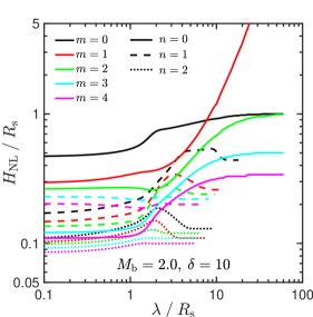
Figure 1: Transition to nonlinearity of different body modes as a function of wavelength. Shown is $H_{\rm NL}$, the maximal displacement of the stream-background interface at the time when fluid crossing first occurs inside the stream, as a function of the perturbation wavelength (both normalized to the stream radius, $R_{\rm s}$) for the case $(M_{\rm b},\delta)=(2,10)$. Different coloured lines correspond to different azimuthal symmetries, $m=0-4$. Different line types correspond to different radial modes, solid lines for the fundamental mode ($n=0$), dashed and dotted lines for the first and second reflected modes ($n=1$ and $2$) respectively. In general, $H_{\rm NL}$ decreases as either $n$ or $m$ are increased. A mode is considered disruptive to the stream if it reaches $H_{\rm NL}\geq R_{\rm s}$. Only the $(m,n)=(1,0);\,(0,0);\,(2,0)$ modes fulfil this criterion, at wavelengths of $\lambda/R_{\rm s}\lower 2.58333pt\hbox{$\;\buildrel>\over{\sim}\;$}8,\,20$, and $40$ respectively. The corresponding KH times for these modes at these wavelengths are $t_{\rm KH}\sim 0.53,\,3.85$, and $1.76t_{\rm sc}$. Therefore, if all modes begin with similar amplitudes, the $(1,0)$ mode will reach $H_{\rm NL}=R_{\rm s}$ first, making it the critical mode. Similar results are found for all $(M_{\rm b},\delta)$ values relevant for cold streams.

Regarding stream deceleration, at $t<t_{\rm NL}$, the stream velocity remains roughly constant. At $t>t_{\rm NL}$, the critical perturbation bends the stream into a sinusoidal shape, effectively driving a piston through the background medium at every crest of the sinusoid. This produces a periodic pattern of weak shocks propagating away from the stream at approximately the speed of sound, $c_{\rm b}$, and fascilitating the transfer of momentum from the stream to the background. The characteristic timescale for this process is the time it takes such an outward propagating wave to encounter a mass of background fluid equal to the initial stream mass. For 2d slabs this means $c_{\rm b}\tau_{\rm body}\rho_{\rm b}=R_{\rm s}\rho_{\rm s}$, so

$$\tau_{\rm body,\,2d}=\delta\frac{R_{\rm s}}{c_{\rm b}}=\frac{\sqrt{\delta}}{2}t_{\rm sc}.$$ (19)

For 3d cylinders this means $[(R_{\rm s}+c_{\rm b}\tau_{\rm body})^{2}-R_{\rm s}^{2}]\rho_{\rm b}=R_{\rm s}^{2}\rho_{\rm s}$, so

$$\tau_{\rm body,\,3d}=\left[\sqrt{1+\delta}-1\right]\frac{R_{\rm s}}{c_{\rm b}}=\frac{\sqrt{1+\delta}-1}{2\sqrt{\delta}}t_{\rm sc}.$$ (20)

For $\delta=1,\,10,\,100$, $\tau_{\rm body,\,3d}/\tau_{\rm body,\,2d}\simeq 0.41,\,0.23,\,0.09$ respectively, the same as for surface modes, since in both cases the difference between $\tau_{\rm 3d}$ and $\tau_{\rm 2d}$ arrises from a purely geometrical effect. Furthermore, while $\tau_{\rm body,\,2d}>t_{\rm sc}$ for $\delta>4$ and reaches $4t_{\rm sc}$ for $\delta=100$, $\tau_{\rm body,\,3d}<t_{\rm sc}$ for any $\delta$, with an assymptotic value of $0.5t_{\rm sc}$ for $\delta\rightarrow\infty$. It is also worth noting that in both 2d and 3d,

$$\frac{\tau_{\rm surface}}{\tau_{\rm body}}=\frac{1+\delta^{-1/2}}{\alpha M_{\rm b}}.$$ (21)

We conclude that stream deceleration due to body modes is much more rapid in 3d than in 2d, especially for dense streams, similar to the conclusion reached for surface modes.

The deceleration process described above is not very efficient. Slabs initially loose roughly $12\%$ of their velocity per $\tau_{\rm body,\,2d}$ at $t\lower 2.58333pt\hbox{$\;\buildrel>\over{\sim}\;$}t_{\rm NL}$, but once the stream breaks this decreases to $\sim 1.6\%$ per $\tau_{\rm body,\,2d}$, before the velocity has reached half its initial value (P18). The origin of these efficiencies is unclear, and we cannot predict from first principles what they might be for 3d cylinders. However, so long as they are not significantly smaller the stream should reach half its initial velocity before the deceleration rate decreases, due to the much smaller ratio of $\tau_{\rm body,\,3d}$ to $t_{\rm sc}$. This will further enhance the effective deceleration rate due to body modes in 3d compared to 2d.

3 Numerical Methods

In this section we describe the details of our simulation code and setup, as well as our analysis method. In §3.7 we compare our setup to that used in P18.

3.1 Hydrodynamic Code

We use the Eulerian AMR code RAMSES (Teyssier, 2002), with a piecewise-linear reconstruction using the MonCen slope limiter (van Leer, 1977) and an HLLC approximate Riemann solver (Toro, Spruce & Speares, 1994), identical to M16 and P18.

3.2 Unperturbed Initial Conditions

One of our main goals is to compare the non-linear evolution of KHI in a two dimensional slab and a three dimensional cylinder under identical initial conditions. For slabs, the simulation domain is a square of side $L=1$, representing the $xz$ plane, extending from $-0.5$ to $0.5$ in both the $x$ and $z$ directions. The slab is centered at $x=0$, such that the stream fluid occupies the region $|x|<R_{\rm s}$, while the background fluid fills the rest of the domain. Analogously, for cylinders, the simulation domain is a cube of side $L=1$, extending from $-0.5$ to $0.5$ in all directions. The cylinder axis is placed along the $z$ axis, at $r=0$. The stream fluid occupies the region $r<R_{\rm s}$ while the background fluid occupies the rest of the domain. We hereafter use standard cylindrical coordinates, $(r,\varphi,z)$, when discussing both 3d and 2d simulations, with the convention that for 2d simulations, $r=|x|$ and $\varphi=0$ or $\pi$ for $x>0$ and $x<0$ respectively.

We set the stream radius to $R_{\rm s}=1/32$ in all simulations. Both fluids are ideal gasses with adiabatic index $\gamma=5/3$, and initial uniform pressure $P_{0}=1$. The background is initialized with density $\rho_{\rm b}=1$ and velocity $\vec{v}_{\rm b}=0$. The stream is initialized with density $\rho_{\rm s}=\delta$ and velocity $\vec{v}_{\rm s}=V\hat{z}=M_{\rm b}c_{\rm b}\hat{z}$, where $c_{\rm b}=\sqrt{5/3}$ is the background sound speed in simulation units. Since the stream and the background are initially in pressure equilibrium, the sound speed in the stream is $c_{\rm s}=\delta^{-1/2}c_{\rm b}$.

In the setup described above, the density and velocity are discontinuous at the interface between the stream and the background. This generates numerical perturbations at the grid scale, which grow faster than the intended perturbations in the linear regime, and may dominate the instability at late times depending on their amplitude. Furthermore, since smaller scales grow more rapidly in the linear regime, these numerical perturbations become more severe as the resolution is increased, preventing convergence of the solution (Robertson et al., 2010). This is remedied by smoothing the unperturbed density and velocity profiles around the interfaces using the ramp function proposed by Robertson et al. (2010), which was also used in M16 and P18,

$$f(r)=f_{\rm b}+\left(f_{\rm s}-f_{\rm b}\right)\times\mathcal{R}(r),$$ (22)

$$\mathcal{R}(r)=\frac{1}{2}\left[1-{\rm tanh}\left(\frac{r-R_{\rm s}}{\sigma}\right)\right],$$ (23)

where $f$ stands for either $\rho$ of $\vec{v}$. This yields $f=f_{\rm s}$ inside the stream, at $r<R_{\rm s}$, while $f=f_{\rm b}$ in the background. The parameter $\sigma$ determines the width of the transition zone. The function $\mathcal{R}(r)$ transitions from $0.05$ to $0.95$ over a full width of $\sim 3\sigma$ in $(r-R_{\rm s})$. For the surface mode simulations presented in §4.1 we adopt $\sigma=R_{\rm s}/32$. For the body mode simulations presented in §4.2 we use values of $\sigma$ ranging from $R_{\rm s}/32$ to $R_{\rm s}/8$ (Table 3).

3.3 Boundary Conditions

We use periodic boundary conditions at $z=\pm 0.5$, and outflow boundary conditions at $x=\pm 0.5$ and $y=\pm 0.5$ (for 3d simulations), such that gas crossing the boundary is lost from the simulation domain. The boundary conditions at $x,\,y=\pm 0.5$ may affect the interface region once a sound crossing time from the interface to the boundary has elapsed. For an interface at $r=R_{\rm s}$, the minimal time for this interaction to occur (assuming shocks in the background dissolve into sound waves quickly) is $T_{\rm box}=(L-2R_{\rm s})/c_{\rm b}\sim 0.73$ in simulation units for $R_{\rm s}=1/32$. All of our simulations were run for between 10-20 stream sound crossing times, $T_{\rm end}=10-20t_{\rm sc}=(10-20)R_{\rm s}/c_{\rm s}\sim(0.48-0.96)\delta^{1/2}$. For $\delta=1$, this is typically less than $T_{\rm box}$, so our results are not influenced by the outflow boundary conditions. However, for $\delta=100$ we have $T_{\rm end}\sim(6.6-13.2)T_{\rm box}$. While we do not explicitly test the influence of the boundary conditions in our 3d simulations, we showed in P18 that this is negligible in 2d simulations with comparable ratios of $T_{\rm end}$ to $T_{\rm box}$.

3.4 Computational Grid

We used a statically refined grid in all runs, with the resolution gradually decreasing away from the stream axis. For most of our runs, the highest resolution region was ${\rm max}(|x|,|y|)<3R_{\rm s}$, with cell size $\Delta=2^{-11}$. For $R_{\rm s}=1/32$ this corresponds to $\Delta=R_{\rm s}/64$, or 128 cells per stream diameter. The cell size increases by a factor of 2 every $3R_{\rm s}$ in the $x$ and $y$-directions, up to a maximal cell size of $2^{-7}$. The resolution is uniform along the $z$ direction, parallel to the stream axis.

Overall, our results are converged in terms of the computational grid. We have tested the dependence of our results to increasing or decreasing the resolution by a factor of 2, such that the cell sizes range from $2^{-12}-2^{-8}$ or $2^{-10}-2^{-6}$ respectively. We have also tested the effect of changing the refinement intervals from $3R_{\rm s}$ to $1.5R_{\rm s}$. These results are presented in Appendix §B.

3.5 Perturbations

We initialize nearly all of our simulations with a random realization of periodic perturbations in the radial component of the velocity, $v_{\rm r}$. In practice, we initialize the following perturbations in the Cartesian components of the velocity,

$$\begin{array}[]{c}v_{\rm x}^{\rm pert}(r,\varphi,z)=\sum_{j=1}^{N_{\rm pert}}v_{\rm 0,j}~{}{\rm cos}\left(k_{\rm j}z+m_{\rm j}\varphi+\phi_{\rm j}\right)\\ \\ \times{\rm exp}\left[-\dfrac{(r-R_{\rm s})^{2}}{2\sigma_{\rm pert}^{2}}\right]{\rm cos}\left(\varphi\right)\end{array},$$ (24)

$$\begin{array}[]{c}v_{\rm y}^{\rm pert}(r,\varphi,z)=\sum_{j=1}^{N_{\rm pert}}v_{\rm 0,j}~{}{\rm cos}\left(k_{\rm j}z+m_{\rm j}\varphi+\phi_{\rm j}\right)\\ \\ \times{\rm exp}\left[-\dfrac{(r-R_{\rm s})^{2}}{2\sigma_{\rm pert}^{2}}\right]{\rm sin}\left(\varphi\right)\end{array}.$$ (25)

In 3d, this results in a perturbation to $v_{\rm r}=v_{\rm x}{\rm cos}(\varphi)+v_{\rm y}{\rm sin}(\varphi)$. In 2d, since $\varphi$ is always $0$ or $\pi$, $v_{\rm y}^{\rm pert}=0$ everywhere, while each individual mode, $j$, in $v_{\rm x}^{\rm pert}$ contributes to both of the slab interfaces. As discussed below, in one simulation we initilized perturbations in the stream-background interface rather than the radial velocity. This has the form

$$r_{\rm s}=R_{\rm s}\left[1+\sum_{j=1}^{N_{\rm pert}}h_{\rm 0,j}~{}{\rm cos}\left(k_{\rm j}z+m_{\rm j}\varphi+\phi_{\rm j}\right)\right].$$ (26)

The velocity perturbations are localized on the stream-background interface, with a penetration depth set by the parameter $\sigma_{\rm pert}$. In all runs with $\sigma=R_{\rm s}/32$ in eq. (23) we used $\sigma_{\rm pert}=R_{\rm s}/16$, while in the runs with $\sigma=R_{\rm s}/8$ presented in §4.2 we used $\sigma_{\rm pert}=R_{\rm s}/8$. However, we experimented with both $\sigma_{\rm pert}=R_{\rm s}/16$ and $R_{\rm s}/8$ and found no noticeable difference in our results.

To comply with periodic boundary conditions, all wavelengths were harmonics of the box length, $k_{\rm j}=2\pi n_{\rm j}$ where $n_{\rm j}$ is an integer, corresponding to a wavelength $\lambda_{\rm j}=1/n_{\rm j}$. In each simulation, we include all wavenumbers in the range $n_{\rm j}=16-64$, corresponding to all available wavelengths in the range $R_{\rm s}/2-2R_{\rm s}$. As discussed below, in one simulation we expanded the wavenumber range to $n_{\rm j}=2-64$, corresponding to all available wavelengths in the range $R_{\rm s}/2-16R_{\rm s}$.

Each perturbation mode is also assigned a symmetry mode, represented by the index $m_{\rm j}$ in eqs. (24) and (25), and discussed in §2. In order to initialize self-consistent perturbations in 2d and 3d, in nearly all simulations we only consider $m=0,1$, as these are the only symmetry modes available in 2d. For each wavenumber $k_{\rm j}$ we include both an $m=0$ mode and an $m=1$ mode. This results in a total of $N_{\rm pert}=2\times 49=98$ modes per simulation. As discussed below, we also performed one 3d simulation where we initialized the full range $m=0-4$ for each wavenumber $k_{\rm j}$, resulting in $N_{\rm pert}=5\times 49=245$ modes.

Each mode is then given a random phase $\phi_{\rm j}\in[0,2\pi)$. The stochastic variability from changing the random phases was extremely small, and is discussed in Appendix §B. The amplitude of each mode, $v_{\rm 0,j}$ was identical, resulting in a white noise specturm. We set the normalization such that the rms amplitude was $0.01c_{\rm s}$. In the one case where the stream-background interface was perturbed, the rms amplitude was set to $0.1R_{\rm s}$.

In Appendix §A we demonstrate that our numerical setup properly captures the behaviour of KHI in cylindrical geometry in the linear regime, both in terms of the linear growth rates, and the convergence to eigenmodes. This serves both as a validation of our code and numerical setup, as well as a test of the predictions presented in M16.

3.6 Tracing the Two Fluids

In order to track the expansion of the stream into the background and the mixing of the two fluids, our simulations include a passive scalar field, denoted by $\psi(r,\varphi,z,t)$. The passive scalar is initialized such that $\psi=1$ in the stream and $\psi=0$ in the background. Since this field is advected with the flow, it serves as a Lagrangian tracer for the fluid in the simulation (which is Eulerian). An element characterized by passive scalar value $\psi$, density $\rho$ and volume $\rm dV$, contains a mass of stream and background fluid given by

$$\rm dm_{s}=\psi\rho\rm dV\qquad\text{and}\qquad\rm dm_{b}=(1-\psi)\rho\rm dV.$$ (27)

Following P18, we use the passive scalar to define the edges of the perturbed region around the initial interface. The volume-weighted average radial profile of the passive scalar in 3d simulations is given by

$$\overline{\psi}_{\rm 3d}(r,t)=\frac{\int_{-L/2}^{L/2}\int_{0}^{2\pi}\psi_{(r,\varphi,z,t)}r~{}{\rm d\varphi\,dz}}{2\pi rL},$$ (28)

while in 2d simulations it is given by

$$\overline{\psi}_{\rm 2d}(r,t)=\frac{\int_{-L/2}^{L/2}\left[\psi_{(x,z,t)}+\psi_{(-x,z,t)}\right]~{}{\rm dz}}{2L},$$ (29)

where as before $r=|x|$. We hereafter omit the subscript 2d or 3d and simply use $\overline{\psi}(r,t)$ with the dimensionality being clear from the context.

Table 2: Parameters of simulations studying the nonlinear evolution of surface modes. The columns show, from left to right, the Mach number of the stream with respect to the background sound speed, $M_{\rm b}$, the density contrast between the stream and the background, $\delta$, the Mach number of the stream with respect to the sum of the two sound speeds, $M_{\rm tot}$ (eq. 2), the number of cells per stream radius, $R_{\rm s}/\Delta$ where $\Delta$ is the cell size in the highest resolution region, and the refinement scheme, where the cell size is increased by a factor of 2 every $\Delta_{\rm ref}$ in the $x$ and $y$-directions. The high resolution region is thus ${\rm max}(|x|,|y|)<\Delta_{\rm ref}$. The smoothing width parameter in eq. (23) was $\sigma=R_{\rm s}/32$ in all cases. The first eight rows, above the horizontal line, represent our fiducial runs presented in this section. The following five rows represent tests to check convergence with respect to resolution and the refinement strategy, and are presented in Appendix §B.

$M_{\rm b}$	$\delta$	$M_{\rm tot}$	$R_{\rm s}/\Delta$	$\Delta_{\rm ref}/R_{\rm s}$
0.1	1	0.05	64	3.0
0.5	1	0.25	64	3.0
1.0	1	0.50	64	3.0
1.5	1	0.75	64	3.0
0.5	10	0.38	64	3.0
1.0	10	0.76	64	3.0
0.5	100	0.45	64	3.0
1.0	100	0.91	64	3.0
1.0	1	0.50	32	1.5
1.0	1	0.50	64	1.5
1.0	1	0.50	128	1.5
1.0	10	0.76	32	3.0
1.0	100	0.91	32	3.0

Initially, each interface is characterized by a sharp transition from $\overline{\psi}=1$ at $r<R_{\rm s}$ to $\overline{\psi}=0$ at $r>R_{\rm s}$. The nonlinear evolution of KHI mixes the fluids near the interface, and the initial discontinuity of $\overline{\psi}_{(r)}$ is smeared over a finite width around each interface (see Fig. 2). The resulting profile is monotonic and can be used to define the edges of the perturbed region around an interface, $r(\overline{\psi}=\epsilon)$ on the background side and $r(\overline{\psi}=1-\epsilon)$ on the stream side, where $\epsilon$ is an arbitrary threshold. The background-side thickness of the perturbed region is then defined as

$$h_{\rm b}\equiv{\rm max_{r}}r(\overline{\psi}=\epsilon)-R_{\rm s},$$ (30)

while the stream-side thickness is defined as

$$h_{\rm s}\equiv R_{\rm s}-{\rm min_{r}}r(\overline{\psi}=1-\epsilon).$$ (31)

The ${\rm max_{r}}$ and ${\rm min_{r}}$ in eqs. (30) and (31) are only necessary to avoid fluctuations in the $\overline{\psi}(r)$ profile, which in practice is smooth and monotonic, especially near the edges. While $h_{\rm b}$ as defined in eq. (30) is always well defined, at late times the perturbed region encompases the entire stream and $\overline{\psi}(r=0)<1-\epsilon$. In this case, we define $h_{\rm s}=R_{\rm s}$. The total width of the perturbed region is given by $h\equiv h_{\rm b}+h_{\rm s}$.

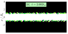
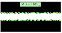
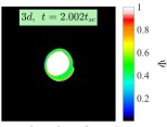
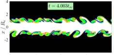
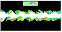
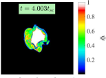
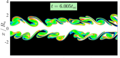
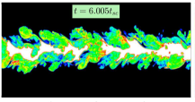
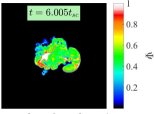
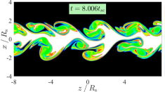
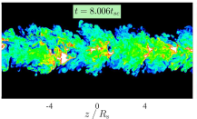
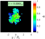
Figure 2: Evolution of surface modes in a 2d slab (left) and a 3d cylinder (centre, and right). Shown are snapshots of $\psi$, a passive scalar field used as a Lagrangian tracer for the stream fluid. The values $\psi=0$ (background) and $\psi=1$ (stream) correspond to cells with a pure fluid composition, while cells with $0<\psi<1$ contain a mixture of both fluids. The unperturbed initial conditions were $(M_{\rm b},\delta)=(1,1)$. The initial perturbations were identical in both simulations and are described in §3. The snapshot times in units of the stream sound crossing time, $t_{\rm sc}=2R_{\rm s}/c_{\rm s}$, are shown in each panel. The left-hand column shows the distribution of $\psi$ in a 2d slab simulation. The center column shows the distribution of $\psi$ in the $xz$ plane of a 3d simulation, an “edge-on” view of the cylinder, while the right-hand column shows the distribution in the $xy$ plane, a “face-on” view. At $t\sim 2t_{\rm sc}$, the edge-on distribution of $\psi$ in the 3d cylinder appears nearly identical to its distribution in the 2d slab simulation, while the face-on distribution is dominated by symmetric, $m=0$, and antisymmetric, $m=1$, modes. At $t=4t_{\rm sc}$, the face-on view of the cylinder reveals higher-order azimuthal modes, though the edge-on view remains similar to the slab. By $t=6t_{\rm sc}$, the structure of the 3d simulation begins to deviate from that of the 2d slab. In 2d, the largest eddies remain coherent and continue to grow while the centre of the stream remains unmixed even at $t=8t_{\rm sc}$. In 3d, by $6t_{\rm sc}$ the largest eddies have broken up and generated small-scale turbulence, and by $8t_{\rm sc}$ there is no unmixed fluid left in the stream. Similar figures showing stream evolution in simulations with different values of $(M_{\rm b},\delta)$ can be found in §D.

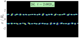
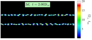
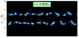
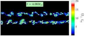
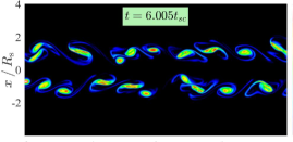
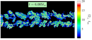
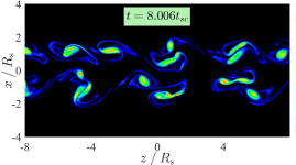
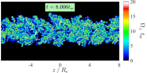
Figure 3: Evolution of vorticity in surface mode simulations of a 2d slab (left) and a 3d cylinder (right). Shown are snapshots of $\Omega_{\perp}$, the magnitude of the vorticity component perpendicular to the stream axis, normalized by the stream sound crossing time. In 2d, $\Omega_{\perp}=|\Omega_{\rm y}|$ while in 3d $\Omega_{\perp}=(\Omega_{\rm r}^{2}+\Omega_{\varphi}^{2})^{1/2}$. The simulation and the snapshots shown are the same as in Fig. 2, and the slices shown are the same as the left-two columns in that figure, namely for the 3d simulation we show a single slice through the $xz$ plane. Similar to the distribution of $\psi$ shown in Fig. 2, at $t\sim 2t_{\rm sc}$ the vorticity in the 3d cylinder appears nearly identical to the 2d slab. At later times, the vortices in the 2d slab merge to form larger vortices which remain coherent until $8t_{\rm sc}$ with no noticeable small scale strcture. On the other hand, in the 3d cylinder the vortices begin to break up and small scale structure is evident already at $4t_{\rm sc}$. By $8t_{\rm sc}$ the medium appears completely turbulent and the largest vortices are barely visible. This exemplifies the qualitative difference between vortex evolution and turbulence generation in two- and three-dimensions.

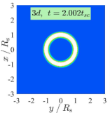
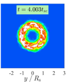
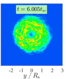
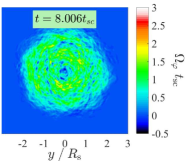
Figure 4: Evolution of mean vorticity in 3d surface mode simulations. Shown are maps of the azimuthal components of the vorticity, $\Omega_{\varphi}$, averaged over the entire length of the box in the $z$ direction and projected onto the $xy$ plane. The simulation and the snapshots shown are the same as in Figs. 2 and 3. At $t=2t_{\rm sc}$, the vorticity is entirely in the azimuthal direction as in an ideal vortex ring, implying that the fluid motion is confined to the $zr$ plane at each azimuthal angle $\varphi$, and consistent with the similarity between the 2d slab and 3d cylinder at this time seen in Figs. 2 and 3. $\Omega_{\rm\varphi}$ remains the dominant component of vorticity through $t=8t_{\rm sc}$, maintaining a ring-like structure within the shearing layer between the two fluids. At $t\geq 4t_{\rm sc}$, small fluctuations in $\Omega_{\rm r}$ and $\Omega_{\rm z}$ are present as well (see text).

The above definitions for $h$, $h_{\rm s}$, and $h_{\rm b}$ depend on $\epsilon$. The exact dependence depends on the $\overline{\psi}(r)$ profile, which varies somewhat with $(M_{\rm b},\delta)$. In general, larger values of $\epsilon$ correspond to smaller values of $h$. We adopt $\epsilon=0.04$ as our fiducial value, though we experimented as well with $\epsilon=0.03$ and $0.02$, which was the fiducial choice in P18. In almost all our simulations the difference between these values was very small, on the order of $\lower 2.58333pt\hbox{$\;\buildrel<\over{\sim}\;$}10\%$. The exceptions are simulations with $\delta=100$, where we find that $h_{\rm s}$ estimated with $\epsilon=0.02$ fluctuates with time rather than monotonically growing. These fluctuations are damped when using $\epsilon=0.04$, and so we adopt this value for all cases.

3.7 Comparison to P18

There are several differences between the numerical setup used in the 2d slab simulations presented here and those presented in P18. Firstly, the fiducial stream radius in P18 was $R_{\rm s}=1/64$ and $1/128$ for surface and body modes respectively, while the cell size in the highest resolution region was $\Delta=2^{-13}$. This yields 256 and 128 cells per stream diameter for surface mode and body mode simulations respectively, while our simulations have 128 cells per diameter for both cases. Furthermore, the high resolution region was much larger in P18 than in our simulations, extending to $10-20R_{\rm s}$. These changes were all necessary in order to make the transition to 3d, and were adopted in our 2d simulations as well for consistency. In Appendix §B, we show that our 3d results are converged with respect to the number of cells per stream diameter and the size of the high resolution region, as was shown in P18 for the 2d case. The only potential effect of making the stream wider with respect to the box is that we are more sensitive to boundary effects. However, as discussed in §3.3, we do not expect this to be an issue.

An additional difference is the width of the initial smoothing layer between the stream and the background (eq. 23). In P18, our fiducial value for $\sigma$ was $R_{\rm s}/128$ for surface modes and $R_{\rm s}/32$ for body modes, while we used $R_{\rm s}/32$ for surface modes and values in the range $R_{\rm s}/32-R_{\rm s}/8$ for body modes. We showed in P18 that the results of 2d simulations were not strongly dependent on the precise value of $\sigma$, so long as this was of order a few cells. However, as we show in §4.2, when $M_{\rm b}>M_{\rm crit}$ the results of 3d simulations depend strongly on the choice of $\sigma$, and for consistency we also adjust the values for our 2d slab simulations.

The most important differences between our setup and that of P18 concern the initial perturbations. We initiate perturbations in the radial component of the velocity dubbed velocity-only perturbations in P18, where the fiducial method of perturbing the stream was interface-only perturbations, periodic perturbations to the shape of the stream-background interface. The onset of shear layer growth or stream deformation requires a perturbation in the stream-background interface to grow to nonlinear amplitude. Before this can happen, the initial velocity perturbation must evolve into eigenmodes and trigger the growth of interface perturbations, which takes of order the perturbation sound crossing time for surface modes and of order the stream sound crossing time for body modes (M16). Furthermore, while we seeded perturbations with wavelengths in the range $(1/2-2)R_{\rm s}$, the wavelength range for surface mode simulations in P18 was $(1/16-1/2)R_{\rm s}$, while for body modes it was $(1/4-16)R_{\rm s}$. Recall that for body modes, the transition to nonlinearity is dominated by the critical perturbation with a wavelength of order $\sim 10R_{\rm s}$ (§2.3). Since our initial conditions contain no power on scales larger than $2R_{\rm s}$, we must wait for the inverse cascade to transfer energy to large scales before the critical perturbation can begin to grow. In P18, on the other hand, the initial conditions already contained power at these scales, so growth could begin immediately. As we will see in §4, both of these effects lead to a delay in the onset of nonlinear growth in our simulations. However, once nonlinear growth begins the evolution is insensitive to the initial perturbations, as was demonstrated in P18. As discussed in §4.2, we explicitly test this by performing one 3d simulation with interface only perturbations (eq. 26) in the wavelength range $(1/2-16)R_{\rm s}$.

4 Simulation Results

We now present the results of our numerical simulations. In §4.1 we address the nonlinear evolution of surface modes. In §4.2 we discuss the nonlinear evolution of body modes and high-$m$ surface modes at $M_{\rm b}>M_{\rm crit}$.

4.1 The Nonlinear Evolution of Surface Modes

The range of parameters studied in the numerical simulations presented in this section is listed in Table 2. These span the range of density contrast and Mach number relevant to cosmic cold streams, $0.5<M_{\rm b}<1.5$ and $1<\delta<100$, and also include an effectively incompressible case with $M_{\rm b}=0.1$. For each case, we simulated both a 3d cylinder and a 2d slab as described in §3. Additionally, we simulated several cases with different resolution or refinement schemes to check convergence. The results of these convergence studies are presented in Appendix §B. All of the results presented in this section are converged with respect to the grid.

4.1.1 Stream Morphology

Figure 2 shows a time sequence of the evolution of the passive scalar field, $\psi$, for the case $(M_{\rm b},\delta)=(1,1)$. We show snapshots at $t/t_{\rm sc}\sim 2$, $4$, $6$, and $8$ for the 2d slab simulation (left), a slice through the $y=0$ plane of a 3d cylinder (an edge-on view, centre), and a slice through the $z=0$ plane of the cylinder (a face-on view, right). At $t\sim 2t_{\rm sc}$, the distribution of $\psi$ in the $xz$ plane of the 3d cylinder appears nearly identical to its distribution in the 2d slab, as expected from §2.2.1. The distribution in the $xy$ plane appears dominated by a combination of symmetric and antisymmetric modes, with $m=0$ and $1$, as initialized. At $t=4t_{\rm sc}$, the edge-on view of the cylinder remains very similar to the slab, with large-scale coherent eddies surrounding a relatively unmixed core. On the other hand, in the face-on view the symmetry seems to have broken and azimuthal modes with $m$ of a few are present. By $t=6t_{\rm sc}$, the structure of the 3d simulation begins to deviate from that of the 2d slab. In 2d, the large-scale eddies remain coherent and continue to grow while the inner $\sim 20\%$ of the slab remains unmixed. On the other hand, in 3d the largest eddies have begun to break-up and cascade towards smaller scales, while the high-$m$ modes continue to grow, generating a more turbulent and mixed structure with very little unmixed fluid in the stream, concentrated along its axis. By $t=8t_{\rm sc}$, the 3d simulation is completely turbulent and the stream contains no unmixed fluid, while in the 2d simulation the largest eddies are still coherent and the inner $\sim 10\%$ of the stream is still relatively unmixed. This highlights that while the initial shear layer growth in 3d cylinders is very similar to 2d slabs, there is a qualitative difference between 2d and 3d, as discussed in §2.2.1. In 2d, there exists only an inverse cascade to larger scales which is why the largest eddies remain coherent and only grow larger as they merge. In 3d, the inverse cascade coexists with a direct cascade to smaller scales which breaks up the largest eddies, generates turbulence, and enhances mixing. Nevertheless, the overall thickness of the shear layer is very similar in 2d and 3d, as predicted in §2.2.1.

4.1.2 Vorticity

Figure 3 compares the evolution of vorticity, $\vec{\Omega}=(\vec{\nabla}\times\vec{v})$, in 2d slab and 3d cylinders. We focus on the same case shown in Fig. 2, $(M_{\rm b},\delta)=(1,1)$, but these results apply to all simulations. We show slices through the $y=0$ plane of the magnitude of the vorticity component perpendicular to the stream axis, at the same times as in Fig. 2. This is $\Omega_{\perp}=|\Omega_{\rm y}|$ and $(\Omega_{\rm r}^{2}+\Omega_{\varphi}^{2})^{1/2}$ in 2d and 3d respectively, and these have been normalized by the stream sound crossing time. Similar to the distribution of $\psi$ seen in Fig. 3, at $t\sim 2t_{\rm sc}$ the vorticity in the 2d and 3d simulations are nearly identical. In the 2d simulation the vorticity remains concentrated in well defined vortices which continue to grow by mergers until $t>8t_{\rm sc}$. However, in the 3d simulation the vortices begin to break up and transfer power to smaller scales already at $t\sim 4t_{\rm sc}$, and by $t=8t_{\rm sc}$ the situation is completely turbulent, with a homogeneous and isotropic distribution of vorticity. This highlights the qualitative difference between vortex evolution and turbulence generation in 2d and 3d discussed above.

Figure 4 shows the evolution of the mean azimuthal component of the vorticity, $\Omega_{\varphi}=(\nabla\times\vec{v})\cdot{\hat{\varphi}}$, in the same 3d simulation and at the same times as shown in Figs. 2 and 3. $\Omega_{\varphi}$ has been averaged over the full length of the box in the $z$ direction and normalized by the stream sound crossing time. This averaging highlights the vorticity of the largest eddies while removing most small scale random motions. At $t=2t_{\rm sc}$, the vorticity is entirely in the $\varphi$ direction and concentrated in a well defined ring, as expected from the discussion in §2.2.1 and consistent with the similarity between the 2d slab and 3d cylinder at this time (Figs. 2 and 3). At later times, the vortex ring expands radially into both the stream and the background as the shear layer grows. Its structure remains relatively coherent, with nearly all of the large-scale vorticity in the $\varphi$ direction. At $t=8t_{\rm sc}$, the volume-weighted mean values of $\Omega_{\rm\varphi}$, $\Omega_{\rm r}$ and $\Omega_{\rm z}$, averaged over the full length of the box and within $r<2R_{\rm s}$, are $\sim 0.77$, $\sim 0.0001$ and $0.0022t_{\rm sc}^{-1}$ respectively, while their standard deviations are $\sim 0.36$, $0.29$ and $0.40t_{\rm sc}^{-1}$. However, in any single slice along $z$, the vorticity is nearly isotropic at $t\lower 2.58333pt\hbox{$\;\buildrel>\over{\sim}\;$}4t_{\rm sc}$, once velocity perturbations in all three directions have grown, as evident in Fig. 3.

Figure 5: Shear layer growth in 2d slabs versus 3d cylinders, for subsonic and transonic streams with respect to the sum of the sound speeds in both fluids, $M_{\rm tot}\leq 1$. On the left we show the penetration of the shearing layer into the stream and the background, $h_{\rm s}/R_{\rm s}$ (solid) and $h_{\rm b}/R_{\rm s}$ (dashed) respectively, as a function of time, $t/t_{\rm sc}$, for a 2d slab (red) and a 3d cylinder (black) with $(M_{\rm b},\delta)=(1.0,10)$. $h_{\rm s}$ behaves similarly in 2d and 3d until it reaches $\sim 0.3R_{\rm s}$, after which it grows $\sim 30\%$ faster in 3d. $h_{\rm b}$ remains extremely similar in 2d and 3d until it reaches $\lower 2.58333pt\hbox{$\;\buildrel>\over{\sim}\;$}1.5R_{\rm s}$, after which the growth rate in 3d is reduced by a factor of $\sim 2$, while the 2d growth rate remains constant. Very similar behaviour is seen in all simulations (see text). The centre panel shows, for all simulations, the average value of the entrainment ratio, $E_{\rm v}=h_{\rm s}/h_{\rm b}$, during the period when $t>2t_{\rm sc}$ and $h_{\rm s}<0.9R_{\rm s}$. Different colours mark different combinations of $(M_{\rm b},\delta)$ while squares and circles mark 3d and 2d simulations respectively. The dashed line shows the analytic prediction, $E_{\rm v}=\delta^{-1/2}$ (eq. 6). While $E_{\rm v}$ is systematically $\sim 30\%$ higher in 3d due to differences in $h_{\rm s}$, the simulation results agree very well with the analytic predictions in both 2d and 3d.

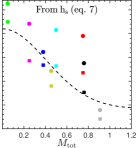
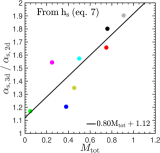
Figure 6: The normalized shear layer growth rate, $\alpha$, as a function of compressibility parametrized by $M_{\rm tot}$. We show the values of $\alpha$ derived using eq. (3) (left), eq. (8) (centre-left), and eq. (7) (centre-right), after measuring $h$, $h_{\rm b}$, and $h_{\rm s}$ as a function of time when $t>2t_{\rm sc}$ and $h_{\rm s}<0.9R_{\rm s}$. Different colours mark different combinations of $(M_{\rm b},\delta)$ while filled squares and circles mark 3d and 2d simulations respectively. Empty squares in the left-hand panel show the results of P18 with error bars denoting the scatter among three random realizations of the initial perturbation spectrum. In our 2d simulations, all three methods for measuring $\alpha$ yield very similar results, which are consistent with both the results of P18 and the empirical fit by Dimotakis (1991) (eq. 4), shown by the dashed line. Using $h_{\rm b}$ to determine $\alpha$ yields very similar results in 2d and 3d simulations, though using $h_{\rm s}$ yields larger values in 3d cylinders. In the right-hand panel we show the ratio of $\alpha_{\rm 3d}$ to $\alpha_{\rm 2d}$ as determined using $h_{\rm s}$. This ratio is roughly proportional to $M_{\rm tot}$, ranging from $\sim(1.1-1.9)$ in the range $M_{\rm tot}\sim(0-1)$. We present the best-fit linear relation with a solid line.

4.1.3 Shear Layer Growth

Figure 5 examines the growth of the shear layer in 2d slab and 3d cylinder simulations. On the left we show the one-sided thicknesses, $h_{\rm b}/R_{\rm s}$ and $h_{\rm s}/R_{\rm s}$, as a function of time for for 2d slab and 3d cylinder simulations with $(M_{\rm b},\delta)=(1.0,10)$. Very similar behaviour is seen in all $(M_{\rm b},\delta)$ combinations. While $h_{\rm s}\lower 2.58333pt\hbox{$\;\buildrel<\over{\sim}\;$}0.3R_{\rm s}$, its behaviour in 2d and in 3d are very similar. At later times, the growth of $h_{\rm s}$ in the 2d simulation undergoes a series of slight stalls where its amplitude is nearly constant for a brief time followed by continued growth at roughly the same rate. This is not seen in the 3d simulations, where $h_{\rm s}$ grows at a roughly constant rate until $h_{\rm s}\sim 0.8R_{\rm s}$ at which point the growth rate increases until the whole stream is engulfed by the shear layer. This may partly be due to the fact that there are many more eddies in a 3d cylinder than a 2d slab, so discrete eddy mergers (the main mechanism for shear layer growth) average out. Furthermore, as $h_{\rm s}$ grows towards the stream axis, the distance between vortex planes along different azimuthal cuts of a cylinder decreases, and interactions between vortex planes may occur, generating turbulence. Overall, $h_{\rm s}\sim(30-40)\%$ larger in 3d than in 2d for most of the evolution. On the other hand, the behaviour of $h_{\rm b}$ is identical in 2d and in 3d until $h_{\rm b}\sim(1.5-2)R_{\rm s}$, consistent with our expectations from §2.2.1. At later times, $h_{\rm b}$ continues to grow at the same rate in 2d, while the growth rate in 3d decreases by a factor of $\sim 2$. In all simulations, the decrease in the growth rate of $h_{\rm b}$ occurs when $h_{\rm b}\sim(1.5-2)R_{\rm s}$, and does not appear to be correlated with a fixed number of sound crossing times or with a fixed decrease in the stream velocity (discussed below). We therefore speculate that it is due to turbulence transfering energy from large to small scales, thereby decreasing the energy available to the largest eddies which drive the shear layer growth. This cascade exists only in 3d, and “kicks in” once the largest eddies have grown comparable to the stream width.

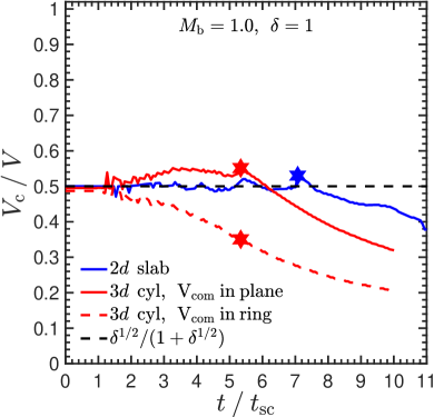
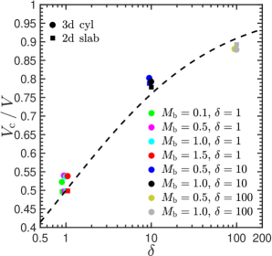
Figure 7: Convection velocity, $V_{\rm c}$, of 2d slabs and 3d cylinders, for subsonic and transonic streams with $M_{\rm tot}\leq 1$. $V_{\rm c}$ is the velocity of the largest eddies in the shear layer between the stream and the background, and is predicted to follow eq. (5), shown by the dashed lines in both panels. In the left-hand panel we show the evolution of $V_{\rm c}$ as a function of time for the simulations with $(M_{\rm b},\delta)=(1,1)$. The blue line shows the 2d slab case, where $V_{\rm c}$ is evaluated by the centre of mass velocity in the shear layer, following P18. This matches the analytic prediction until $h_{\rm s}=R_{\rm s}$, which is marked by the blue star. The red lines represent the 3d cylinder simulation. The solid line shows the centre of mass velocity in the shear layer within a planar slice through the stream midplane, following eq. (33), while the dashed line shows the centre of mass velocity within the full cylindrical shear layer, following eq. (34). The former matches the analytic prediction until $h_{\rm s}=R_{\rm s}$, marked by the red star, while the latter is systematically lower and monotonically decreasing from $t\lower 2.58333pt\hbox{$\;\buildrel>\over{\sim}\;$}t_{\rm sc}$. The right-hand panel shows the results for all simulations as a function of density contrast, averaged when $t>2t_{\rm sc}$ and $h_{\rm s}<0.9R_{\rm s}$. Symbols are as in Fig. 5. The results closely follow the analytic prediction, in both 2d and 3d.

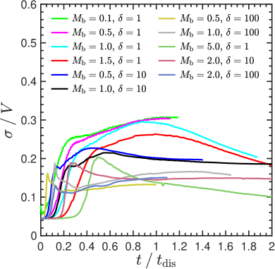
Figure 8: Turbulence induced by shear layer growth. We show the turbulent velocities inside the shear layer as a function of time for all 3d simulations unstable to surface modes. These include three simulations with $M_{\rm b}>M_{\rm crit}$ that are unstable to high-$m$ surface modes, discussed in §4.2. The turbulent velocities, $\sigma$, have been normalized to the initial stream velocity, $V$, while the time has been normalized to the disruption time, $t_{\rm dis}$, when the shear layer consumes the entire stream. All simulations, regardless of $M_{\rm b}$ and $\delta$, follow the same trend. The turbulence increases at early times, reaches a peak value of $\sigma/V\sim 0.2-0.3$ at early times, and then decreases to an assymptotic value of $\sigma/V\lower 2.58333pt\hbox{$\;\buildrel<\over{\sim}\;$}0.2$. 2d slab simulations do not exhibit such universal behaviour.

In the right panel of Fig. 5 we show the entrainment ratio (eq. 6) for all simulations, both 2d and 3d. These were evaluated at $t>2t_{\rm sc}$ and while $h_{\rm s}<0.9R_{\rm s}$, following an initial transient phase and before the behaviour of $h_{\rm s}$ becomes too stochastic. We show for comparison the analytic prediction $E_{\rm v}=\delta^{-1/2}$ (eq. 6). Our simulations match the analytic prediction very well, and in all cases the 3d results are very similar to the 2d results. There is a systematic trend for $E_{\rm v}$ to be $\sim(30-40)\%$ larger in 3d than in 2d. This is driven primarily by $h_{\rm s}$ being larger in 3d, while $h_{\rm b}$ is very similar in 2d and 3d, as seen in the left-hand panel and described above.

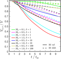
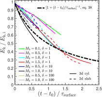
Figure 9: Deceleration and dissipation of bulk kinetic energy in streams due to surface modes, for subsonic and transonic streams with $M_{\rm tot}\leq 1$. In the left and centre panels, we show the centre of mass velocity of the stream fluid (weighted by the passive scalar $\psi$) normalized by its initial value, as a function of time for all simulations. Different colours mark the different combinations of $(M_{\rm b},\delta)$. Solid and dashed lines show the results of 3d and 2d simulations respectively. In the left-hand panel the time axis is normalized by the sound crossing time, which is the same in 2d and 3d. Clearly, 3d cylinders decelerate much faster than 2d slabs in all cases, though the time at which deceleration begins, $t_{0}$, is of order the sound crossing time in all cases. In the right-hand panel we renormalize the time axis by the predicted deceleration timescales, $\tau_{\rm surface}$, given by eq. (10) and eq. (12) for 2d and 3d respectively. For $\alpha$, we use eq. (4) for 2d slabs and 3d cylinders with $\delta<8$, while for 3d cylinders with $\delta>8$ we use half that value (see text for details). Both the 2d and 3d simulations reach half their initial velocity at $t\sim t_{0}+\tau_{\rm surface}$, as predicted. The thick dot-dashed line in the right-hand panel shows the predicted velocity profile from eq. (38). Except for the cases with $\delta=1$ and $M_{\rm b}\leq 1$, which are the least relevant for cold streams, the model is a good match to the simulated results. In the right-hand panel, we show the total kinetic energy associated with laminar flow of both stream and background fluid normalized by its initial value, as a function of time normalized by $\tau_{\rm surface}$. The rate of dissipation of bulk kinetic energy in 3d cylinders is extremely similar to the stream deceleration rate, as predicted.

Figure 6 shows the value of $\alpha$ (eq. 3) measured in our simulations. Similar to $E_{\rm v}$, these were evaluated at $t>2t_{\rm sc}$ and while $h_{\rm s}<0.9R_{\rm s}$. As discussed in P18, $\alpha$ is expected to be mainly a function of the compressibility, and is empirically found to correlate with $M_{\rm tot}$, shown on the $x$ axis. We show the values of $\alpha$ measured from the simulations in three different ways, using the total width of the shear layer, $h$, following eq. 3 (left), using the one-sided thickness in the background, $h_{\rm b}$, following eq. 8 (centre-left), and using the one-sided thickness in the stream, $h_{\rm s}$, following eq. 7 (centre-right). We note that the growth of $h_{\rm s}$ is related to stream disruption (eq. 9), while the growth of $h_{\rm b}$ is related to stream deceleration (eqs. 10 and 12). In the left hand panel, we also show the results from P18 (figure 7), where the error bars represent the scatter obtained in three random realizations of the initial perturbation spectrum. For comparison, in each panel we show the empirical fit proposed by Dimotakis (1991) (eq. 4). When measuring the full width of the shear layer (left), the results of our 2d simulations are roughly consistent with eq. (4), at least to the same degree as the results of P18. In fact, our results at $\delta=100$ are actually more consistent with eq. (4) than those of P18. However, for $\delta=1$ the values of $\alpha$ measured in this way are systematically higher in 3d simulations. This is due to the more rapid growth of the shear layer into the stream, which is a larger fraction of the total shear layer growth for smaller $\delta$. Therefore, when using $h_{\rm b}$ to determine $\alpha$, as in the centre panel, the results of 3d and 2d simulations are in excellent agreement, though we stress that $\alpha$ here is measured primarily when $h_{\rm b}<2R_{\rm s}$, before the growth rate in 3d simulations decreases by a factor of 2 relative to 2d simulations, as discussed above. On the other hand, when using $h_{\rm s}$ to determine $\alpha$ in the centre-right panel, the discrepancy between 2d and 3d is much larger, with the ratio $\alpha_{\rm 3d}/\alpha_{\rm 2d}$ scaling roughly linearly with $M_{\rm tot}$, as shown in the right-most panel. We find the best-fit linear relation to be

$$\frac{\alpha_{\rm s,\,3d}}{\alpha_{\rm s,\,2d}}\simeq 0.80M_{\rm tot}+1.12,$$ (32)

which is shown by the solid line in the right-most panel of Fig. 6.

We conclude that shear layer growth in 3d cylinders is overall very similar to 2d slabs, as expected, though the penetration into the stream is systematically more rapid following eq. (32). Furthermore, similar to P18, we conclude that the shear layer growth rate is reasonably well fit by eq. (4), which is an excellent match to our simulations at high and low values of $M_{\rm tot}$, and shows a $\sim 50\%$ non-systematic discrepancy at intermediate values. As discussed in Appendix B of P18, eq. (4) does appear to fit experimental data better than numerical simulations. The reasons for this are not entirely clear, and left for future study. However, since the shear layer growth rate is linear with $\alpha$, such a non-systematic $50\%$ discrepancy will be negligible compared to other uncertanties in our model when applied to astrophysical scenarios in §5, and also when compared to the systematic differences between 2d slabs and 3d cylinders.

4.1.4 Convection Velocity

Figure 7 examines the convection velocity, $V_{\rm c}$ (eq. 5), the typical velocity of the largest eddies in the shear layer. In P18 we showed that in 2d slab simulations this could be evaluated from the centre of mass velocity of the fluid inside the shear layer, shown as the blue line in the left-hand panel for the case $(M_{\rm b},\delta)=(1,1)$. All other simulations show similar behaviour. The 2d result is consistent with the analytic prediction, shown by the dashed line, until the shear layer encompasses the entire stream, $h_{\rm s}=R_{\rm s}$, marked by the star. Based on the discussion in §2.2.1, we expect that for 3d cylinders the same will be true for the centre of mass velocity of the fluid in the shear layer in a 2d slice through the stream axis at constant $\varphi$. The scatter between different $\varphi$ values is very small, as expected, of the order of a few percent. Therefore, we average over all angles to obtain better statistics. In practice, we compute

$$V_{\rm com,\,in\,plane}=\dfrac{\int_{R_{\rm s}-h_{\rm s}}^{R_{\rm s}+h_{\rm b}}\overline{\rho}_{(r)}\widetilde{v_{\rm z}}_{(r)}~{}{\rm dr}}{\int_{R_{\rm s}-h_{\rm s}}^{R_{\rm s}+h_{\rm b}}\overline{\rho}_{(r)}~{}{\rm dr}},$$ (33)

where the density profile, $\overline{\rho}(r)$, is obtained analogously to eq. (28), and the velocity profile is density-weighted, i.e. $\widetilde{v_{\rm z}}\equiv\overline{\rho v_{\rm z}}/\overline{\rho}$. This is shown by the red solid line in the left-hand panel of Fig. 7, and closely matches the analytic prediction and the 2d result, until $h_{\rm s}=R_{\rm s}$ which is marked by the red star. Clearly, this is different than computing the centre of mass velocity within the cylindrical shear layer, given by

$$V_{\rm com,\,in\,ring}=\dfrac{\int_{R_{\rm s}-h_{\rm s}}^{R_{\rm s}+h_{\rm b}}\overline{\rho}_{(r)}\widetilde{v_{\rm z}}_{(r)}r~{}{\rm dr}}{\int_{R_{\rm s}-h_{\rm s}}^{R_{\rm s}+h_{\rm b}}\overline{\rho}_{(r)}r~{}{\rm dr}},$$ (34)

and shown by the red dashed line in the same panel. While this begins at similar values to the prediction for $V_{\rm c}$ at $t\lower 2.58333pt\hbox{$\;\buildrel<\over{\sim}\;$}t_{\rm sc}$, it decreases monotonically in time. Given the similarity between 2d slabs and slices through 3d cylinders discussed above, we speculate that $V_{\rm c}$ may still be associated with the drift velocity of the largest eddies in the shear layer of 3d cylinders, as it is for 2d slabs (§2.2.1). We thus conclude that the largest eddies in a cylindrical shear layer move faster than the centre of mass velocity within the shearing ring.

In the right-hand panel of Fig. 7 we show the convection velocity measured in all our simulations as a function of the density contrast. These were evaluated at $t>2t_{\rm sc}$ and while $h_{\rm s}<0.9R_{\rm s}$, similar to Fig. 5. The results in 2d and 3d are extremely similar, and both follow the analytic prediction of eq. (5), shown by the dashed line. This strengthens the picture described in §2.2.1, further highlighting the similarity of shear layer growth in 2d slabs and 3d cylinders.

4.1.5 Turbulence

The growth of the shear layer drives turbulence, fascilitating the mixing of the two fluids. This can be seen visually in Fig. 2 (and in Fig. 12 discussed in §4.2). We evaluate the magnitude of turbulence within the shear layers in our 3d cylinder simulations as

$$\sigma^{2}=\dfrac{\int_{R_{\rm s}-h_{\rm s}}^{R_{\rm s}+h_{\rm b}}\overline{\rho}_{(r)}\left[(v_{\rm z}-\widetilde{v_{\rm z}}_{(r)})^{2}+v_{\rm x}^{2}+v_{\rm y}^{2}\right]r~{}{\rm dr}}{\int_{R_{\rm s}-h_{\rm s}}^{R_{\rm s}+h_{\rm b}}\overline{\rho}_{(r)}\,r~{}{\rm dr}}.$$ (35)

We subtract the longitudinal velocity at each radius in order to remove any ordered shear inherited from the initial conditions and focus on small scale turbulence.

In Fig. 8 we show the evolution of $\sigma/V$, where $V=M_{\rm b}c_{\rm b}$ is the initial stream velocity, for all 3d cylinder simulations studied here, as well as three simulations with $M_{\rm b}>M_{\rm crit}$ that are unstable to high-$m$ surface modes, discussed in §4.2 below. The latter have $(M_{\rm b},\delta)=(5,1),\,(2,10),\,(2,100)$. The time axis in Fig. 8 has been normalized by $t_{\rm dis}$, the time when the shear layer consumes the entire stream, i.e. when $h_{\rm s}=R_{\rm s}$. All simulations follow the same trend. $\sigma/V$ increases to a maximum of $\sim 0.2-0.3$ at early times, and then decays to an assymptotic value of $\sigma/V\lower 2.58333pt\hbox{$\;\buildrel<\over{\sim}\;$}0.2$. Simulations with larger $\delta$ peak at smaller values and at earlier times, but the variance is small considering the range of $\delta$ values simulated. Weighting the density in eq. (35) (and in the evaluation of the shearing profile $\widetilde{v_{\rm z}}_{(r)}$) by the passive scalar $\psi$ in order to focus on turbulent motions of the stream fluid yields very similar results at late times, $t>t_{\rm dis}$, showing that at these late times both fluids are well mixed within the shear layer. Note that this means that one cannot directly infer the total turbulent energy relative to the initial kinetic energy of the stream from Fig. 8, because the mass contained within the shear layer grows with time, such that at $t>t_{\rm dis}$ the mass contained within the shear layer is larger than the initial stream mass. In practice, we find in all simulations that the total turbulent energy assymptotes at $\sim 10\%$ of the initial kinetic energy of the stream.

Fourier analysis reveals that on scales $\lower 2.58333pt\hbox{$\;\buildrel<\over{\sim}\;$}R_{\rm s}$, the turbulence is very close to isotropic for all cases. We defer a more detailed analysis of the turbulence to future work which will include radiative cooling, as well as the gravity of the halo into which the stream is flowing which may be an additional source of turbulence (see §6). We note that 2d slabs do not exhibit such universal evolution. At $t\sim t_{\rm dis}$, $\sigma/V$ varies by more than a factor of 3 and does not have a well defined maximum for $\delta>1$. However, since it is well known that turbulence manifests itself in a qualitatively different way in 2d than in 3d, we do not dwell on this comparison here.

4.1.6 Deceleration and Kinetic Energy Dissipation

In Fig. 9 we show the deceleration of streams in 2d slab and 3d cylinder simulations. We evaluate this by computing the centre of mass velocity of stream fluid,

$$V_{\rm z,s}=\dfrac{\int_{0}^{L/2}\overline{\psi}_{(r)}\,\overline{\rho}_{(r)}\,\widetilde{v_{\rm z}}_{(r)}\,r~{}{\rm dr}}{\int_{0}^{L/2}\overline{\psi}_{(r)}\,\overline{\rho}_{(r)}\,r~{}{\rm dr}}.$$ (36)

In the left-hand panel we show the stream velocity normalized to its initial value, $V$, as a function of time normalized by the stream sound crossing time. It is evident that 3d cylinders decelerate faster than 2d slabs, as predicted in §2.2.1. However, the time at which deceleration begins is very similar in 2d and 3d for all cases. We denote this time as $t_{0}$, and define it as the time when the stream velocity has dropped to $98\%$ its initial value. For all values of $(M_{\rm b},\delta)$, we find $t_{0}\sim 0.5-1.5t_{\rm sc}$.

Table 3: Parameters of simulations with $M_{\rm tot}>1$ (eq. 2), studying the nonlinear evolution of body modes and of high-$m$ surface modes. The columns show, from left to right, the Mach number of the stream with respect to the background sound speed, $M_{\rm b}$, the density contrast between the stream and the background, $\delta$, the Mach number of the stream with respect to the sum of the two sound speeds, $M_{\rm tot}$, the number of cells per stream radius, $R_{\rm s}/\Delta$ where $\Delta$ is the cell size in the highest resolution region, the ratio of the stream radius to the smoothing parameter $\sigma$ (eq. 23), and the refinement scheme (see Table 2 for details). The first three rows in the table represent simulations with the same smoothing as in those presented in §4.1. The following six represent simulations with more aggressive smoothing of the initial conditions. The next five rows represent tests to check convergence with resolution and refinement strategy, and are presented in Appendix §B. The final two rows represent simulations where the initial perturbation spectrum was changed, as described in the text. For these two models, only a 3d cylinder was simulated.

$M_{\rm b}$	$\delta$	$M_{\rm tot}$	$R_{\rm s}/\Delta$	$R_{\rm s}/\sigma$	$\Delta_{\rm ref}/R_{\rm s}$	Note
5.0	1	2.50	64	32	3.0
2.0	10	1.52	64	32	3.0
2.0	100	1.82	64	32	3.0
5.0	1	2.50	64	8	1.5
2.5	5	1.72	64	8	1.5
2.0	10	1.52	64	16	1.5
2.0	10	1.52	64	8	1.5
2.5	20	2.04	64	8	1.5
2.0	100	1.82	64	8	1.5
2.0	10	1.52	32	32	1.5
2.0	10	1.52	64	32	1.5
2.0	10	1.52	128	32	1.5
2.0	10	1.52	32	8	1.5
2.0	10	1.52	128	8	1.5
5.0	1	2.50	64	32	3.0	$m=0-4$
2.5	5	1.72	64	8	1.5	eq. (26), $16R_{\rm s}$

In the centre panel of Fig. 9, we rescale the time axis by the predicted deceleration timescale, $\tau_{\rm surface}$, given by eq. (10) and eq. (12) for 2d and 3d respectively. Before rescaling the time axis, we move its origin to $t_{0}$ in order to focus on the deceleration itself rather than the “incubation” period before it begins. For the value of $\alpha$ in the expressions for $\tau_{\rm surface}$, we use eq. (4) for 2d slabs and 3d cylinders with $\delta<8$, while for 3d cylinders with $\delta>8$ we use half this value to account for the fact that the growth rate of $h_{\rm b}$ in 3d cylinders decreases by a factor of $\sim 2$ once $h_{\rm b}\sim 2R_{\rm s}$. This occurs at $\sim\tau_{\rm surface}$ for $\delta\sim 8$, while for denser streams it happens earlier. Since the deceleration rate is proportional to the background mass flux into the shear layer, which is proportional to $(R_{\rm s}+h_{\rm b})^{2}$, we approximate that all the deceleration occurs with the reduced value of $\alpha$. This approximation is valid for cold streams with $\delta>10$. As can be seen from the centre panel of Fig. 9, when scaled to the predicted deceleration timescales, the results of 2d and 3d simulations are in agreement, and the stream velocity decreases to half its initial value at $t\sim\tau_{\rm surface}$, as predicted.

The curvature in the deceleration profiles can be approximated by the following simple toy model. We assume that the deceleration can be modeled as

$$\frac{{\rm d}V_{\rm s}}{{\rm d}t}=-\frac{V_{\rm s}}{\tau_{\rm surface}}=-\frac{\alpha\sqrt{\delta}}{(1+\sqrt{\delta})(\sqrt{1+\delta}-1)}\frac{V_{\rm s}^{2}}{R_{\rm s}},$$ (37)

where $V_{\rm s}(t)$ is the time-dependent stream velocity, and the final equality is valid for 3d cylinders using eq. (12) for $\tau_{\rm surface}$, which we now assume to be time dependent through $V_{\rm s}$ rather than constant. An analogous expression can be derived for 2d slabs using eq. (10). The solution to eq. (37) with the initial condition $V_{\rm s}(t=0)=V_{0}$ is

$$V_{\rm s}(t)=V_{0}(1+t/\tau_{\rm surface,\,0})^{-1},$$ (38)

where $\tau_{\rm surface,\,0}$ is the inital value of $\tau_{\rm surface}$, i.e. with the initial stream velocity $V_{0}$. Eq. (38) is valid for both 3d cylinders and 2d slabs. We show this model as the thick dash-dotted line in the centre panel of Fig. 9. Except for the cases with $\delta=1$ and $M_{\rm b}\leq 1$, where the flow is subsonic with respect to the sound speed in the stream and which are the least relevant for actual cold streams, this simple model is a good fit to the simulations. The subsonic cases can be brought into good agreement with the model if we lower the value of $\alpha$ used in $\tau_{\rm surface}$ by a factor $\sim 2/3$. This seems to imply that for subsonic flow, the transfer of momentum from the stream to the background in the shearing layer is not instantaneous, which was implicit in the derivation of $\tau_{\rm surface}$. For higher Mach number flows, shocks fascilitate the momentum transfer.

In addition to stream deceleration, we wish to evaluate the decrease of kinetic energy associated with laminar streaming motions, of both stream and background fluid. This is not obviously inferred from the left and centre panels of Fig. 9, since the stream transfers some of its momentum to the background gas as it decelerates. As noted above, the stream decelerates by distributing its initial momentum over more and more mass as background fluid is continuously added to the shear layer. If the material within the outer envelope of the shear layer moves at a characteristic velocity $v$, and the total mass within this region is $m$, we thus have

$$\dot{v}/v\sim-\dot{m}/m.$$ (39)

Since the kinetic energy associated with this streaming motion is $E_{\rm K}\propto mv^{2}$, we have

$$\frac{\dot{E_{\rm K}}}{E_{\rm K}}\sim\frac{\dot{v}}{v}.$$ (40)

Making the simplifying assumption that the characteristic velocity in the outer shear layer, $v$, is equal to the stream velocity, $V_{\rm s}$, we thus predict that the kinetic energy associated with the laminar flow of stream and background fluid decreases at the same rate as the stream velocity. While this assumption is clearly simplified, since there is a velocity profile within the shear layer, it actually reproduces the kinetic energy loss seen in simulations rather well. This is shown in the right-hand panel of Fig. 9, where we plot the kinetic energy normalized by its initial value as a function of time normalized by $\tau_{\rm surface}$. The kinetic energy is evaluated from the simulations as

$$E_{\rm K}=\pi~{}\int_{0}^{L/2}\overline{\rho}_{(r)}\,\widetilde{v_{\rm z}}_{(r)}^{2}\,r~{}{\rm dr},$$ (41)

where by using $\widetilde{v_{\rm z}}_{(r)}$ we are focusing only on the laminar flow, without turbulent motions. We note that the results are identical whether we limit the integration in eq. (41) to $r=R_{\rm s}+h_{\rm b}$ rather than $L/2$, showing that there is no bulk laminar flow in the background outside the shear layer. By comparing the centre and right-hand panels of Fig. 9 we see that for 3d cylinders the total bulk kinetic energy decreases at a very similar rate to the stream velocity, as predicted by our simple toy model. We also note that in 2d slabs, the kinetic energy seems to decrease at a slower rate. This implies that the background fluid accreted onto the shear layer does not mix as efficiently in 2d, and moves at an overall slower velocity than the bulk of the stream fluid.

As the bulk kinetic energy decreases, it is transferred into several channels. Some of it goes into turbulent motions, though as discussed in relation to Fig. 8, this only accounts for $\sim 10\%$ of the initial kinetic energy in our simulations. Additional channels for the lost kinetic energy are thermal energy, of both the stream and background fluids, and sound waves which propagate away from the stream and may eventually leave the simulation domain. We defer a detailed analysis of the relative importance of these various channels to future work which will include radiative cooling (Mandelker et al., in prep.). In particular, we will address there what fraction of the lost kinetic energy is eventually dissipated into radiation. For the moment, all we can say is that eq. (40) and Fig. 9 represent an upper limit to the total energy that may be dissipated and subsequently radiated due to KHI.

4.2 The Nonlinear Evolution of Body Modes

We now turn to study streams with $M_{\rm tot}>1$, i.e. streams which are supersonic with respect to the sum of the sound speeds in both fluids. As described in §2, in 2d such streams are dominated by body modes as surface modes stabilize, while in 3d there exist unstable surface modes with azimuthal modes $m>1$. The numerical simulations presented in this section is listed in Table 3. These span the range of density contrast and Mach number relevant to cosmic cold streams, $2.0<M_{\rm b}<2.5$ and $10<\delta<100$, with additional simulations at lower density contrast and higher Mach number, $\delta=1,\,5$ and $M_{\rm b}=5$, in order to test the general validity of our results. For each case, we simulated both a 3d cylinder and a 2d slab as described in §3. Furthermore, we examine the effect of varying the width of the initial smoothing layer, parametrized by $\sigma$ in eq. (23), as well as several cases with different resolution or refinement scheme to check convergence, and present these results in Appendix §B. Finally, we performed two simulations where we varied the initial perturbation spectrum. In the first of these we included azimuthal modes with $m=(0-4)$ instead of $m=(0-1)$. In the second we initiated perturbations to the stream-background interface following eq. (26) rather than to the radial velocity, and extended the wavelength range to $(0.5-16)R_{\rm s}$ rather than $(0.5-2)R_{\rm s}$ (see §3.5). Unlike all other cases, these final two models include only 3d cylinder simulations.

We stress that varying the width of initial transition layer, $\sigma$, is not merely a numerical test, but rather has physical meaning, since increasing the width of the transition layer damps short wavelength perturbations. This has been described in §3.2 and is demonstrated below. In reality, the width will be determined by additional physics, such as thermal conduction, diffusion, or the radial accretion of gas onto the stream. As none of these processes are included in our current simulations, we vary $\sigma$ as a crude way to test this effect, delaying a more detailed consideration of these physical processes to future work (see §6).

4.2.1 Appearance of high-$m$ modes

In Fig. 10 we show the effects of varying the width of the initial smoothing layer. We show slices through the $z=0$ plane of a 3d simulation with $(M_{\rm b},\delta)=(2,10)$, using three different values for $\sigma$: $R_{\rm s}/32$, which was the value used in the simulations presented in §4.1, $R_{\rm s}/16$ and $R_{\rm s}/8$. For each case, we show a snapshot shortly after the shearing layer between the stream and the background begins to expand, marked by the growth of $h_{\rm b}$ in Fig. 11 below. This happens at $t/t_{\rm sc}\sim 1.5$, $2.6$, and $5.2$ for $R_{\rm s}/\sigma=32$, $16$, and $8$ respectively. The dominant modes at these times appear to be $m\sim 12$, $m=6$ and $m=4$, corresponding to azimuthal wavelengths $\lambda_{\rm\varphi}=2\pi R_{\rm s}/m\sim 0.5R_{\rm s}$, $1.0R_{\rm s}$, and $1.6R_{\rm s}$. For $\delta=10$, $M_{\rm crit}\sim 1.77$ (eq. 1). Therefore, according to eq. (13), for $M_{\rm b}=2$ and longitudinal wavelengths $\lambda=2R_{\rm s}$, the longest wavelength in the initial perturbation spectrum, surface modes are unstable for $m>2$. However, the initial smoothing layer suppresses the growth of surface modes where either $\lambda$ or $\lambda_{\varphi}$ is of order the smoothing layer thickness, $\sim(3-4)\sigma$, or smaller. For $\sigma=R_{\rm s}/32$, the total width of the smoothing layer is $\lower 2.58333pt\hbox{$\;\buildrel>\over{\sim}\;$}0.1R_{\rm s}$, which substantially reduces the growth rates of surface modes with $\lambda_{\rm\varphi}\lower 2.58333pt\hbox{$\;\buildrel<\over{\sim}\;$}0.5R_{\rm s}$, i.e. $m\lower 2.58333pt\hbox{$\;\buildrel>\over{\sim}\;$}12$ making this the fastest growing mode. Increasing $\sigma$ by a factor of 2 increases the shortest unstable wavelength by a factor of $\sim 2$, which in turn decreases the growth rate of the fastest growing mode by a factor of $\sim 2$ because $\omega\propto k$ for surface modes. This is consistent with both the dominant mode and with the time when it dominates the stream morphology for $\sigma=R_{\rm s}/16$ and $R_{\rm s}/8$. We note that in the latter case, while the $m=4$ surface mode does eventually dominate the stream morphology, this only occurs after the critical body mode perturbation has become nonlinear, so the transition to nonlinearity is dominated by body modes even though the nonlinear phase contains a mix of both surface and body modes.

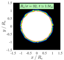
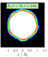
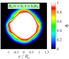
Figure 10: Excitation of high-$m$ surface modes in cylinders with $M_{\rm b}>M_{\rm crit}$. Shown are slices through the $z=0$ plane of a simulation with $(M_{\rm b},\delta)=(2,10)$, with different values of the smoothing parameter used in eq. (23), $\sigma/R_{\rm s}=1/32$ (left), $1/16$ (centre), and $1/8$ (right). colour shows the value of the passive scalar $\psi$, as in Fig. 2. For each case, we show a snapshot shortly after $h_{\rm b}$ has begun to grow (see Fig. 11), at $t\sim 1.5$, $2.6$ and $5.2t_{\rm sc}$ respectively. The dominant modes are $m\sim 12$, $m=6$ and $m=4$. Based on eq. (13), at a longitudinal wavelength of $\lambda=2R_{\rm s}$, the largest wavelength seeded in the initial perturbation, surface modes are unstable for $m>2$. However, the smoothing layer with $\sigma=R_{\rm s}/32$ suppresses the growth of surface modes with $\lambda\lower 2.58333pt\hbox{$\;\buildrel<\over{\sim}\;$}0.5R_{\rm s}$. The azimuthal wavelength associated with mode number $m$ is $\lambda_{\rm\varphi,\,m}=2\pi R_{\rm s}/m$, which is $\sim 0.5R_{\rm s}$ for $m=12$, explaining why this is the dominant mode in the left-hand panel. Increasing $\sigma$ by a factor of $2$ increases the shortest unstable wavelength by a factor of $2$, resulting in a decrease in the dominant $m$ by a factor of $\sim 2$, as seen in the other two panels. Since $t_{\rm KH}\propto\lambda$ for surface modes, this also leads to a factor of $\sim 2$ reduction in growth rate, consistent with the simulation results.

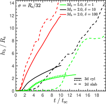
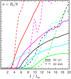
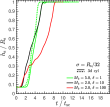
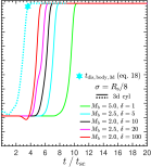
Figure 11: Expansion and shear layer growth in streams where $M_{\rm b}>M_{\rm crit}$ (eq. 1). We show $h_{\rm b}/R_{\rm s}$ in the left two panels and $h_{\rm s}/Rs$ in the right two panels, each as a function of time normalized by the stream sound crossing time, $t_{\rm sc}=2R_{\rm s}/c_{\rm s}$. The first and third panels from the left show simulations with a narrow initial smoothing layer, $\sigma=R_{\rm s}/32$, while the second and fourth panels show simulations with a wide initial smoothing layer, $\sigma=R_{\rm s}/8$. The large initial values of $h_{\rm s}$ and $h_{\rm b}$ in the simulations with $\sigma=R_{\rm s}/8$ are due to the initial smoothing of the contact discontinuity, which extends to roughly $1.5\sigma$ in each medium. Solid lines in all panels represent 3d simulations while dashed lines in the two $h_{\rm b}$ panels represent 2d simulations (not shown in the two $h_{\rm s}$ panels). Different colours represent different combinations of $(M_{\rm b},\delta)$ (the colour legend in the second and fourth panels is the same). The dotted lines represent simulations with a different initial perturbation spectrum (Table 3). The 2d simulations behave similarly for both values of $\sigma$, though the onset of expansion is slighly delayed in the case with large $\sigma$. In the case with $\sigma=R_{\rm s}/8$, the 2d expansion rates are roughly constant until $h_{\rm b}\sim(8-10)R_{\rm s}$. The 3d simulations with $\sigma=R_{\rm s}/8$ behave similarly to their 2d counterparts at early times, though they begin expanding slightly earlier. The simulation with interface perturbations at long wavelengths (dotted cyan line) begins expanding at $t_{\rm NL}$ predicted from eq. (16) (see text), and is destroyed, in the sense that $h_{\rm s}=R_{\rm s}$, at $t_{\rm dis,\,body,\,3d}$ predicted from eq. (18), which is marked with a star in the rightmost panel. This is unlike its counterpart with velocity perturbations at shorter wavelengths (solid cyan line). Unlike in 2d, the 3d expansion rates decrease once $h_{\rm b}\lower 2.58333pt\hbox{$\;\buildrel>\over{\sim}\;$}2R_{\rm s}$, similar to the simulations described in §4.1, while a shear layer rapidly penetrates into the stream, consuming it within $1-2t_{\rm sc}$. When $\sigma=R_{\rm s}/32$, the 3d simulations become dominated by high-$m$ surface modes before body modes develop. As a result, $h_{\rm s}$ and $h_{\rm b}$ begin growing at $t\sim 1-2t_{\rm sc}$ and are initially well fit by eqs. (7)-(8) with $\alpha=0.05$. The shear layer consumes the stream within $4-5t_{\rm sc}$. The simulation which was initiated with $m=0-4$ modes (dotted green line) is extremely similar to its counterpart with $m=0-1$ (solid green line).

4.2.2 Stream Expansion and Shear Layer Growth

In the left two panels of Fig. 11 we examine the evolution of the stream thickness in 2d slabs and 3d cylinders with $\sigma=R_{\rm s}/32$ and $R_{\rm s}/8$. For body modes, the onset of rapid expansion of the stream can in principle be predicted from eq. (16). However, this assumes an initial perturbation in the stream-background interface at the critical wavelength ($\lower 2.58333pt\hbox{$\;\buildrel>\over{\sim}\;$}10R_{\rm s}$ in all cases), with an initial amplitude $H_{0}$. This was the case in the body mode simulations presented in P18, where perturbations in the stream-background interface were seeded with a spectrum extending out to $16R_{\rm s}$ and constant initial amplitude for each seeded wavelength. As a result, $t_{\rm NL}$ could be directly evaluated from the initial conditions, and coincided with the onset of rapid stream expansion seen in the simulations (P18, figure 17). However, as highlighted in §3.7, this is not the case in most of the simulations presented here, where we seeded perturbations in the radial velocity with wavelengths not exceeding $2R_{\rm s}$. Before the critical perturbation can be excited, interface perturbations at the critical wavelength must be excited. This is discussed further below.

However, we did perform one simulation with interface perturbations at wavelengths up to $16R_{\rm s}$ (see Table 3). This is shown as the dotted cyan line in the second and fourth panels from the left of Fig. 11. This simulation consisted of 126 modes with an rms amplitude of $0.1R_{\rm s}$ (§3.5), yielding an amplitude per wavelength of $\sim 0.009R_{\rm s}$. The critical wavelength in this case is $\sim 9R_{\rm s}$ with a KH time of $\sim 0.55t_{\rm sc}$ (see Table 1). According to eq. (16), this corresponds to $t_{\rm NL}\sim 2.6t_{\rm sc}$, in excellent agreement with the onset of rapid stream expansion. Furthermore, the predicted time for stream disruption based on eq. (18) is $\sim 3.6t_{\rm sc}$, which is marked by the star in the right-most panel of Fig. 11 and is in excellent agreement with the time at which $h_{\rm s}=R_{\rm s}$. Once the stream begins expanding, its expansion rate is extremely similar to that of a simulation with identical parameters but fiducial initial perturbations, shown by the solid cyan line. We therefore conclude that while our fiducial initial perturbations lead to a delayed onset of stream expansion, the subsequent behaviour is well captured.

While we cannot predict the precise disruption times in our fiducial simulations with velocity perturbations, we can qualitatively understand the order in which they disrupt and the approximate ratios between their disruption times. These stem primarily from the fact that the initial radial velocity perturbation amplitudes correspond to different interface dispacement amplitudes for different values of $M_{\rm b}$ and $\delta$. In Appendix §C we derive the displacement amplitude corresponding to a given radial velocity perturbation amplitude and wavelength. As shown there, if the amplitude of the radial velocity perturbation at the critical wavelength is the same for all simulations, and defining $t_{\rm NL}$ as unity for $(M_{\rm b},\delta)=(5.0,1)$, then for $(M_{\rm b},\delta)=(2.5,5),\>(2.0,10),\>(2.5,20)$, and $(2.0,100)$ we have $t_{\rm NL}\sim 0.73,\>0.68,\>0.67,\>0.62$. In the simulations, stream expansion begins at $t\sim 0.72,\>0.61,\>0.50,\>0.33$ relative to the $(M_{\rm b},\delta)=(5.0,1)$ simulation. Our estimate is thus in good quantitative agreement with the simulation results for $(M_{\rm b},\delta)=(2.5,5)$, and in reasonable agreement for $(M_{\rm b},\delta)=(2.0,10)$. As $M_{\rm s}=\delta^{1/2}M_{\rm b}$ is increased, our estimate overshoots the ratio in simulations by a larger amount. This is because our estimate is based on the incorrect assumption that all simulations begin with the same radial velocity amplitude at the critical wavelength. While the amplitude is the same in the seeded wavelength range of $(0.5-2.0)R_{\rm s}$, the critical wavelength at $\sim 10R_{\rm s}$ is excited after one sound crossing time has elapsed due to shocks in the stream. These shocks are stronger for larger Mach number flows (with respect to the stream sound speed), leading to larger initial amplitudes of radial velocity which correspond to larger initial amplitudes in the interface displacement, which result in shorter $t_{\rm NL}$. The details of how exactly the critical wavelength is triggered are beyond the scope of this paper. However, the qualitative agreement of this analysis with the simulation results together with the quantitative agreement in the case where we seeded the simulation with long wavelength interface perturbations, as well as the analogous analysis presented in P18 for the 2d case, lead us to conclude that our predictions for stream disruption due to body modes from §2.3 are supported by numerical simulations.

The 2d simulations behave qualitatively similar with both values of $\sigma$, though the onset of growth in $h_{\rm b}$ is slightly delayed in the simulations with larger $\sigma$, by $\sim(1-2)t_{\rm sc}$ in all cases. We note that in the case with $\sigma=R_{\rm s}/8$, all 2d simulations exhibit very similar growth rates when time is normalized by $t_{\rm s}=R_{\rm s}/V$ (not shown), roughly $h_{\rm b}/R_{\rm s}\sim(0.15-0.2)\times t/t_{\rm s}$. This is sensible, since once the critical mode has taken over and the stream has begun to expand, the stream sound crossing time is no longer meaningful. Rather, the time scale dominating stream evolution is naturally $t_{\rm s}$.

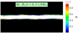
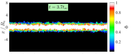
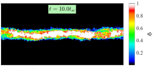
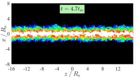
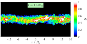
Figure 12: Nonlinear stream evolution and disruption by high-$m$ surface modes vs. body modes. We show slices through the $y=0$ plane of a simulation with $(M_{\rm b},\delta)=(5,1)$, with two different values of the smoothing parameter (eq. 23), $\sigma/R_{\rm s}=1/32$ (left), and $1/8$ (right). Colour shows the value of the passive scalar $\psi$, as in Fig. 2. For each case, the top row shows a snapshot just as $h_{\rm b}$ begins to grow (Fig. 11), while the middle and bottom rows show snapshots 1 and 2 sound crossing times later, respectively. When $\sigma=R_{\rm s}/32$, the stream-background interface is dominated by small-scale structure when $h_{\rm b}$ begins growing, at $t\sim 2.7t_{\rm sc}$. The ensuing growth of $h_{\rm b}$ is due to an expanding shear layer, as in the surface mode simulations described in §4.1. At $\sim 4.7t_{\rm sc}$ there is still an unmixed core at the centre of the stream, which does not fully mix until $t\sim 6.5t_{\rm sc}$. On the other hand, when $\sigma=R_{\rm s}/8$, the stream-background interface is dominated by a large-scale sinusoidal perturbation with relatively little small scale structure when $h_{\rm b}$ begins growing, at $t\sim 9t_{\rm sc}$. By $t\sim 10t_{\rm sc}$ a sinusoidal structure with $\lambda\sim 16R_{\rm s}$ clearly dominates, in agreement with the predicted critical perturbation (§2.3). However, at the same time small scale structure has begun to develop, due to unstable surface modes with high-$m$. Within one additional sound crossing time these small-scale perturbations have efficiently mixed the stream and the background fluids, though the large scale sinusoidal mode is still visible. By $t\sim 11.5t_{\rm sc}$ there is no unmixed fluid left in the stream. Similar figures showing stream evolution in simulations with different values of $(M_{\rm b},\delta)$ can be found in §D.

Unsurprisingly, the dependence of the 3d simulations on $\sigma$ is more significant. When $\sigma=R_{\rm s}/32$, stream expansion in all three simulations begins at $(1-2)t_{\rm sc}$, similar to the surface mode simulations. The initial growth rate of $h_{\rm b}$, until it reaches $\sim 2R_{\rm s}$, is consistent with eq. (8) with $\alpha\sim 0.05$, as expected from eq. (4). We note that a simulation initiated with $m=(0-4)$ modes (dotted green line) is extremely similar to the corresponding simulation with $m=0-1$ only (solid green line). However, when $\sigma=R_{\rm s}/8$ and high-$m$ surface modes are suppressed, stream expansion in 3d begins only shortly before the corresponding 2d simulation. The ratio of onset times in 3d versus 2d simulations is $\lower 2.58333pt\hbox{$\;\buildrel<\over{\sim}\;$}0.7$, roughly consistent with the shorter $t_{\rm KH}$ for the critical perturbation in cylindrical versus slab geometry. Unlike the 2d simulations, which maintain a roughly constant growth rate until $h_{\rm b}\sim(8-10)R_{\rm s}$, the growth rate of $h_{\rm b}$ in 3d simulations declines smoothly once $h_{\rm b}\lower 2.58333pt\hbox{$\;\buildrel>\over{\sim}\;$}2R_{\rm s}$. In the case of $\delta=1$, $h_{\rm b}$ seems to have saturated at a maximal value of $\sim 3.5R_{\rm s}$. As we shall see below, similarly to what was seen in §4.1, the decline in the stream expansion rate coincides with the onset of turbulence, which transfers energy from the large scales driving the stream expansion, to the small scales efficiently mixing the stream and background fluids. It is not entirely clear why the decrease in the growth rate of $h_{\rm b}$ in 3d cylinders compared to 2d slabs seems so much larger here than it did for surface modes (see Fig. 5). However, we recall that for body modes in 2d slabs, $h_{\rm b}$ does not expand due to shear layer growth but rather due to the global deformation of the stream into a long wavelength sinusoidal, so the expansion mechanism is completely different. We defer a more detailed study of this to future work.

In the right two panels of Fig. 11 we examined the penetration of the shear layer into the stream, $h_{\rm s}/R_{\rm s}$, for simulations with $\sigma=R_{\rm s}/32$ and $R_{\rm s}/8$. We only show here results for 3d cylinders, since $h_{\rm s}$ is not a particularly meaningful quantity for body modes in slabs. As detailed in P18 and described in §2.3, shear layer growth is suppressed for body modes, and stream disruption appears through global deformation of the stream into a large sinusoidal shape. However, this is not the case for 3d cylinders due to the appearance of high-$m$ surface modes which create a shear layer that penetrates into the stream (see also Fig. 12 below). The onset of shear layer penetration into the stream is coincident with the onset of rapid expansion. As mentioned above, in simulations with $\sigma=R_{\rm s}/32$ (second panel from the right) the shear layer is well described by eqs. (8) and (7) with $\alpha=0.05$, and in practice for the stream parameters studied here the shear layer consumes the entire stream $\sim(4-5)t_{\rm sc}$ after the onset of growth. On the other hand, simulations with $\sigma=R_{\rm s}/8$ show much more rapid shear layer growth after the onset, with the stream fully consumed within $\sim(1-2)t_{\rm sc}$, consistent with eq. (18) (see also Fig. 12 below). As noted above, the simulation with interface perturbations at wavelengths up to $16R_{\rm s}$, shown by the dashed cyan line, reaches $h_{\rm s}=R_{\rm s}$ at the predicted stream disruption time from eq. (18), which is marked by the cyan star.

4.2.3 Stream Morphology

In Fig. 12 we compare the stream morphology in simulations with $\sigma=R_{\rm s}/32$ and $R_{\rm s}/8$, at the onset of stream expansion. We focus on the case $(M_{\rm b},\delta)=(5,1)$, but the results presented apply to all other cases. We show a slice edge-on through the midplane of the stream, in the $y=0$ plane, just as $h_{\rm b}$ begins growing, $t\sim 2.7t_{\rm sc}$ and $9t_{\rm sc}$ for $\sigma=R_{\rm s}/32$ and $R_{\rm s}/8$ respectively. For each simulation we also show two additional snapshots, one and two sound crossing times after the first. The simulation with narrow smoothing is dominated by small scale structure concentrated at the stream-background interface. This is visible in the first snapshot, and expands with time into both the stream and the background, forming a stratified structure with an unmixed core surrounded by a mixed shear layer. This shear layer is formed by high-$m$ surface modes, and obeys the same physics as described in §4.1. By $t\sim 6.5t_{\rm sc}$ the shear layer has consumed the entire stream. This implies a disruption time of $\sim 3.8t_{\rm sc}$ from the onset of shear layer growth, consistent with eq. (9) with $\alpha\sim 0.05$.

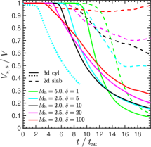
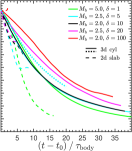
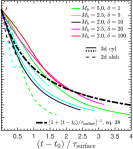
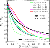
Figure 13: Deceleration and dissipation of bulk kinetic energy in streams due to body modes, for supersonic streams with $M_{\rm b}>M_{\rm crit}$. In the left three panels, we show the centre of mass velocity of the stream fluid (weighted by the passive scalar $\psi$) normalized by its initial value, as a function of time for all body mode simulations with $\sigma=R_{\rm s}/8$. Line styles and colours are the same as in Fig. 11. In the leftmost panel time is normalized by the sound crossing time. The deceleration begins together with the growth of $h_{\rm b}$ (Fig. 11). With the exception of $\delta=1$, the 3d cylinders have decelerated significantly more than the 2d slabs by the end of the simulation at $20t_{\rm sc}$. In the second panel from the left, we renormalize the time axis by the predicted body mode deceleration timescale, $\tau_{\rm body}$ (eq. 19 and eq. 20 for 2d and 3d respectively), and show all curves beginning at $t_{0}$, the time when the velocity has reached $0.95$ its initial value. The 2d simulations all follow the same slope at first, roughly $V_{\rm z,\,s}\sim-0.1Vt/\tau_{\rm body}$. The deceleration rate sharply declines once $h_{\rm b}\sim(8-10)R_{\rm s}$, which is almost always before the slab reaches half its initial velocity. The increase in slab velocity at $t>15t_{\rm sc}$ for the simulation with $\delta=100$ is due to stream fluid leaving the simulation domain and is not to be trusted. Similarly, the 3d simulations all have very similar slopes, roughly $V_{\rm z,\,s}\sim-0.05Vt/\tau_{\rm body}$. While the simulation with $\delta=100$ has a shallower slope at first, it coincides with the other simulations once $V_{\rm z,\,s}/V\lower 2.58333pt\hbox{$\;\buildrel<\over{\sim}\;$}0.75$. The transition of 3d simulations to a shallower slope always occurs after the stream reaches half its initial velocity. In the third panel, we renormalize the time axis by the predicted deceleration timescale for surface modes, $\tau_{\rm surface}$ (eq. 10 and eq. 12 for 2d and 3d respectively), and again show all curves beginning at $t_{0}$. The 3d simulations all roughly follow the predicted velocity profile for surface modes from eq. (38), shown by the thick dot-dashed line, though this is not as good a match for 2d slabs. This is consistent with the late time evolution of 3d cylinders, after the critical body mode begins to grow, being dominated by high-$m$ surface modes and efficient mixing (Fig. 12). In the rightmost panel, we show the total kinetic energy associated with laminar flow of both stream and background fluid normalized by its initial value, as a function of time normalized by $\tau_{\rm surface}$. The rate of dissipation of bulk kinetic energy in 3d cylinders is extremely similar to the stream deceleration rate, as predicted.

On the other hand, in the simulation with wide smoothing, there is very little small-scale structure present at the onset of stream expansion, at $t=9t_{\rm sc}$. Rather, the stream is dominated by a sinusoidal wave with a wavelength of $\lambda\sim 16R_{\rm s}$, consistent with the critical perturbation for this case which is the fundamental helical mode [$(m,n)=(1,0)$] with $\lambda_{\rm crit}\sim 13R_{\rm s}$. After a sound crossing time, the critical perturbation has clearly taken over and the stream is dominated by a large sinusoidal wave with an amplitude of $\lower 2.58333pt\hbox{$\;\buildrel>\over{\sim}\;$}R_{\rm s}$. At the same time, small-scale turbulence has appeared throughout the stream, triggerred by unstable high-$m$, long wavelength surface modes. Within less than one additional sound crossing time, this turbulence has consumed the entire stream. While the long wavelength sinusoidal is still visible, the stream has effectively dissintegrated and mixed with the background. The total disruption time from the onset of shear layer growth is thus $<2t_{\rm sc}$, shorter than the case with narrow smoothing, which was dominated by surface modes from the beginning. The accelerated shear layer growth in this case is likely due to the increased surface area of the stream-background interface caused by the large scale sinus wave. Of course, we recall that the onset of shear layer growth was significantly delayed in this case, until after the critical perturbation had grown. Finally, we note that the turbulent velocities in the shear layer exhibit the same behaviour as in the surface mode simulations shown in Fig. 8, increasing to a maximum of $\sim 0.2-0.3$ at early times, and then decaying to an assymptotic value of $\sigma/V\lower 2.58333pt\hbox{$\;\buildrel<\over{\sim}\;$}0.2$.

4.2.4 Deceleration and Kinetic Energy Dissipation

In Fig. 13 we show the stream deceleration in 2d slab and 3d cylinder simulations with $\sigma=R_{\rm s}/8$. In the leftmost panel we show the stream velocity as a function of time normalized by the stream sound crossing time. For all cases, deceleration begins together with stream expansion and the growth of $h_{\rm b}$ in Fig. 11. Clearly, stream deceleration is more rapid in 3d. The only exception is the case with $\delta=1$, where the final stream velocity in 2d and 3d are comparable. For $\delta\geq 10$, the stream velocity at the end of the 3d simulations is a factor $\sim 3-4$ lower than in the 2d simulations, where the deceleration rate greatly decreases once $h_{\rm b}\sim(8-10)R_{\rm s}$ (see Fig. 11), consistent with the results of P18. The apparent increase in stream velocity in the 2d simulation with $\delta=100$ at $t>15t_{\rm sc}$ is due to stream material leaving the box at this time, and is not to be trusted. All other simulations end before any stream material leaves the box. We note that the simulation initiated with interface perturbations at long wavelengths (dotted cyan line) has a very similar deceleration rate to the corresponding simulation with the same parameters but a fiducial perturbation spectrum (solid cyan line), though it begins decelerating earlier, in agreement with the discussion following Fig. 11.

In the second panel of Fig. 13, we normalize the time axis to $\tau_{\rm body}$ from eq. (19) or eq. (20) for 2d and 3d respectively. Before rescaling the time axis, we move its origin to $t_{0}$, defined as the time when the velocity reaches $0.95$ of its original value, in order to focus on the deceleration itself rather than the “incubation” period before it begins. When scaled in this way, all the 2d simulations exhibit the same behaviour. The initial deceleration rate, while $h_{\rm b}<8R_{\rm s}$, is approximately $V_{\rm z,\,s}\sim-0.1Vt/\tau_{\rm body,\,2d}$, consistent with the results of P18. The 3d simulations with $\delta\leq 10$ all exhibit the same behaviour as well, though different from their 2d counterparts. The stream velocity approximately follows $V_{\rm z,\,s}\sim-0.05Vt/\tau_{\rm body,\,3d}$, meaning that deceleration is half as efficient per $\tau_{\rm body}$ in 3d cylinders than in 2d slabs, though this timescale is objectively much shorter in 3d than in 2d. The cases with $\delta\geq 20$ exhibit slightly shallower slopes, though we note that the simulation with $\delta=100$ exhibits the same slope as those with $\delta\leq 10$ once the velocity has decreased to $\sim 0.75$ its initial value. Similar to the 2d simulations, the deceleration rate in 3d eventually decreases, but this only occurs once the velocity has decreased to less than half its initial value. Unlike the 2d simulations, the decrease in the deceleration rate in 3d is not associated with a critical $h_{\rm b}$, but rather with a decrease in the growth rate of $h_{\rm b}$, coincident with the onset of small scale turbulence and mixing.

Based on the discussion above, a 3d cylinder reaches half its initial velocity in $\sim 10\tau_{\rm body}$. Based on eq. (21), the ratio between this and $\tau_{\rm surface}$ is $\sim 2(1+\delta^{-1/2})/Mb$, where we have assumed $\alpha=0.05$. For $\delta\lower 2.58333pt\hbox{$\;\buildrel>\over{\sim}\;$}10$ and $M_{\rm b}\sim 2$ this ratio is $\sim 1$. Indeed, when plotted against $t/\tau_{\rm surface}$ with $\alpha=0.05$, the different 3d simulations align just as well as when plotted against $t/\tau_{\rm body}$, as seen in the third panel of Fig. 13. The streams reach half their initial velocity at $t\sim\tau_{\rm surface}$, and are reasonably well fit by our toy model for stream deceleration due to surface modes, eq. (38). We conclude that it is equally valid to describe 3d cylindrical streams as decelerating due to shear layer mixing with the appropriate effective growth rate, consistent with the efficient mixing following the growth of the critical perturbation seen in Fig. 12. Based on Fig. 13, this desctription is less satisfactory for 2d slab simulations, as expected.

In the rightmost panel of Fig. 13, we show the total kinetic energy associated with laminar flow, evaluated according to eq. (41), and normalized to its initial value. The bulk kinetic energy decreases at the same rate as the stream velocity, as was the case for surface modes (Fig. 9), and as predicted by our simple toy model of shear layer growth and accretion of background material which begins flowing at roughly the same velocity as the stream (eq. 40). This further supports the description of 3d cylindrical streams as decelerating due to shear layer mixing with the appropriate effective growth rate, as described above.

5 Application to Cold Streams in Massive SFGs at High-$z$

In this section we use the analytic theory of §2, which is broadly supported by our simulations presented in §4, to predict the effect of KHI on cold streams feeding massive galaxies at high redshift. We begin in §5.1 by providing estimates for the relevant stream parameters. In §5.2 we estimate the potential for stream disruption, and in §5.3 we address the effect on their inflow rate.

5.1 Stream Parameters

Our predictions depend primarily on three dimensionless parameters: The Mach number, $M_{\rm b}$, the density contrast, $\delta$, and the ratio of stream radius to the halo virial radius, $R_{\rm s}/R_{\rm v}$. These were crudely estimated in M16 and refined in P18, based on simple analytic arguments and cosmological simulations. We repeat the main arguments here for completeness, and refer the reader to P18 (section 5.1) for further details.

The stream velocity is proportional to the halo virial velocity, which can be related to the sound speed of gas at the virial temperature, yielding $M_{\rm b}\sim 1$. The density contrast is obtained by assuming pressure equilibrium between hot gas at $T_{\rm b}\sim T_{\rm v}$, the virial temperature of an NFW halo, and cold gas at $T_{\rm s}\sim 10^{4}{\rm K}$, set by the steep drop in the cooling rate below that temperature (Sutherland & Dopita, 1993). If both the halo and the stream are roughly isothermal, then this ratio is constant throughout the halo. In practice, the stream temperature can be as high as $\sim 3\times 10^{4}{\rm K}$ due to photo-heating from the UV background (e.g. Goerdt et al., 2010), while the post-shock temperature in the hot halo near $R_{\rm v}$ may only be $\sim 0.5T_{\rm v}$ (Dekel & Birnboim, 2006, P18). Finally, the stream radius is related to its velocity and density through the mass accretion rate along the stream, ${\dot{M}}_{\rm s}\simeq\pi R_{\rm s}^{2}\rho_{\rm s}V_{\rm s}$. Cosmological simulations suggest that this is typically a fixed fraction of the total accretion rate onto the halo virial radius (Danovich et al., 2012), which is constrained by cosmology (e.g. Dekel et al., 2013). The final expressions, including uncertainties in model parameters, are

$$M_{\rm b}\simeq 0.75-2.25,$$ (42)

$$\delta\simeq(10-100)\times M_{12}^{2/3}(1+z)_{3}^{-1},$$ (43)

$$\frac{R_{\rm s}}{R_{\rm v}}\simeq(0.01-0.1)\times\left(\delta_{75}M_{\rm b,1.5}\right)^{-1/2},$$ (44)

where $M_{12}=M_{\rm v}/10^{12}M_{\odot}$, $(1+z)_{3}=(1+z)/3$, $\delta_{75}=\delta/75$ and $M_{\rm b,1.5}=M_{\rm b}/1.5$. We note that $\delta\sim 10$ implies that the backgrond gas has a temperature of $\sim 3\times 10^{5}\,{\rm K}$, which would make it thermally unstable unless it is illuminated by a very hard ionizing background (e.g. Efstathiou, 1992, though see also Binney, Nipoti & Fraternali, 2009 who argue that buoyancy effects may stabilize the halo against thermal instability even without a photoionizing source). This implies that $\delta\lower 2.58333pt\hbox{$\;\buildrel>\over{\sim}\;$}30$ is likely the most physically plausible regime.

5.2 Stream disruption

For 2d slabs, stream disruption manifests itself in different ways for surface and body modes. For the former, disruption occurs when the shear layer consumes the entire slab, while for the latter the stream expads to several times its initial width and breaks up before significant mixing occurs. However, for 3d cylinders there is no such distinction. Even if body modes dominate the transition to nonlinearity, small scale surface modes quickly develop and efficiently mix the stream and background fluids after the critical perturbation takes over (Fig. 12).

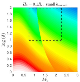
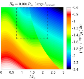
Figure 14: The critical stream radius for disruption due to KHI, $R_{\rm s,dis}$, as a function of $M_{\rm b}$ and $\delta$. Streams with $R_{\rm s}<R_{\rm s,dis}$ are expected to dissintegrate in the CGM before reaching the central galaxy. The critical radius is given by either eq. (45) or eq. (46), depending on whether surface or body modes dominate the instability, as described in the text. The two panels represent two extreme limits for the regime where body modes are unstable, $M_{\rm b}>(1+\delta^{-1/2})$. In the left-hand panel, the initial amplitude of the critical body mode is assumed to be large, $H_{0}=0.1R_{\rm s}$, and the initial smoothing layer between the stream and the background is small enough to allow high-$m$ surface modes to grow, so both surface and body modes are unstable. In the right-hand panel, the initial amplitude of the critical perturbation is assumed to be small, $H_{0}=0.001R_{\rm s}$, and the initial smoothing layer is large enough to stabilize all surface modes when $M_{\rm b}>M_{\rm crit}$ (eq. 1), so only body modes are unstable in this regime. When $M_{\rm b}<(1+\delta^{-1/2})$, these two limits are identical by definition. At larger Mach numbers, the critical radii in the left-hand panel are a factor of $\sim 2$ larger than those in the right-hand panel throughout the range of $(M_{\rm b},\delta)$ values relevant for cold streams, marked by dashed squares. $R_{\rm s,dis}$ ranges from $\sim(0.005-0.05)R_{\rm v}$, decreasing towards higher $\delta$ and higher $M_{\rm b}$, save for a jump to larger values when body modes destabilize. This is $\sim 70\%$ larger than the corresponding range of critical radii for disruption of 2d slabs.

In 2d slabs, surface modes lead to stream disruption after a time $\sim t_{\rm dis,\,surface,\,2d}$ (eq. 9), with $\alpha_{\rm s,\,2d}$ given by eq. (4), where the subscript $s$ denotes that this value of $\alpha$ corresponds to the penetration of the shear layer into the stream rather than the background. However, we find in our simulations that the penetration of the shear layer into 3d cylinders is more rapid than in 2d slabs (Fig. 6, right-two panels), leading to disruption by $t_{\rm dis,\,surface,\,3d}\sim(\alpha_{\rm s,\,2d}/\alpha_{\rm s,\,3d})~{}t_{\rm dis,\,surface,\,2d}$, where the ratio of $\alpha$ values is given by eq. (32). Since the largest eddies in the shear layer move at the convection velocity, $V_{\rm c}$ (eq. 5), the shear layer will consume the stream before reaching the halo centre if $t_{\rm dis,\,surface,\,3d}\leq R_{\rm v}/V_{\rm c}$. Following P18, we write this as a condition on the stream radius, $R_{\rm s}\leq R_{\rm s,dis}^{\rm surface}$, where

$$\frac{R_{\rm s,dis}^{\rm surface}}{R_{\rm v}}=\frac{\alpha_{\rm s,\,3d}(M_{\rm b},\delta)}{\sqrt{\delta}}.$$ (45)

If the instability is initially dominated by body modes, stream disruption occurs after $t_{\rm dis,\,body,\,3d}$ (eq. 18), roughly one sound crossing time after the critical perturbation becomes nonlinear (see Fig. 12). Since body modes cause negligible deceleration prior to this, the stream disintegrates prior to reaching the halo centre if $t_{\rm dis,\,body,\,3d}\leq R_{\rm v}/V$, or $R_{\rm s}\leq R_{\rm s,dis}^{\rm body}$ where

$$\frac{R_{\rm s,dis}^{\rm body}}{R_{\rm v}}=\left[2\sqrt{\delta}M_{\rm b}\left(0.5~{}{\rm ln}\left(\dfrac{R_{\rm s}}{H_{0}}\right)+1\right)\right]^{-1}.$$ (46)

Note that unlike eq. (45), this depends on the initial conditions through the initial amplitude of the critical perturbation, $H_{0}$.

If $M_{\rm b}<(1+\delta^{-1/2})$, then $M_{\rm tot}<1$ (eq. 2) and body modes are stable, so the critical radius for stream disruption is $R_{\rm s,dis}^{\rm surface}$. If $(1+\delta^{-1/2})<M_{\rm b}<M_{\rm crit}=(1+\delta^{-1/3})^{3/2}$ (eq. 1), surface and body modes are both unstable, and the critical stream radius for disruption is given by ${\rm max}(R_{\rm s,dis}^{\rm surface},\,R_{\rm s,dis}^{\rm body})$. If $M_{\rm crit}<M_{\rm b}$, the behaviour depends on the width of the initial smoothing layer between the stream and background fluids, $h_{\rm smooth}$. This width is set by various physical processes, such as thermal conduction or the dynamics of cylidrical accretion onto the stream outside the halo. Simple estimates using Spitzer (1956) conductivity show that it may vary from $h_{\rm smooth}\sim R_{\rm s}$ to $h_{\rm smooth}<<R_{\rm s}$, depending on whether one uses densities and temperatures characteristic of the cold streams or the hot background (M16). A more accurate determination of $h_{\rm smooth}$ is beyond the scope of this paper, and we instead examine two limits. If $h_{\rm smooth}>>2\pi R_{\rm s}/m_{\rm crit}$, with $m_{\rm crit}$ given by eq. (13), then surface modes are stable and the critical radius for stream disruption is $R_{\rm s,dis}^{\rm body}$. However, if $h_{\rm smooth}\lower 2.58333pt\hbox{$\;\buildrel<\over{\sim}\;$}2\pi R_{\rm s}/m_{\rm crit}$, then both surface and body modes are unstable, and the critical stream radius for disruption is given by ${\rm max}(R_{\rm s,dis}^{\rm surface},\,R_{\rm s,dis}^{\rm body})$.

Figure 14 shows the resulting critical stream radius for disruption, $R_{\rm s,dis}/R_{\rm v}$, as a function of $M_{\rm b}$ and $\delta$. The two panels show two extreme limits for the body mode regime. In the left-hand panel, the initial amplitude of the critical perturbation is assumed to be large, $H_{0}=0.1R_{\rm s}$, and the initial smoothing layer between the stream and the background is assumed to be small so that both surface and body modes are unstable. On the other hand, in the right-hand panel, the initial amplitude of the critical perturbation is very small, $H_{0}=0.001R_{\rm s}$, and the initial smoothing layer is large so surface modes are stable. The behaviour at $M_{\rm tot}<1$ is identical in these two limits by definition. At larger Mach numbers, the critical radius in the former limit is a factor of $\sim 2$ larger than in the latter limit throughout the parameter range relevant for cold streams, marked by a dashed square in each panel. We find that streams with radius up to $\sim 0.05R_{\rm v}$ may disentegrate prior to reaching the galaxy. The critical radius ranges from $R_{\rm s,dis}\sim(0.005-0.05)R_{\rm v}$, decreasing with $\delta$, and tending to decrease with $M_{\rm b}$ as well save for a jump to larger values when body modes destabilize. For 2d slabs, the critical radius for disruption was found to range from $\sim(0.003-0.03)R_{\rm v}$ (P18), so moving to 3d has increased the potential for stream disruption by $\sim 70\%$.

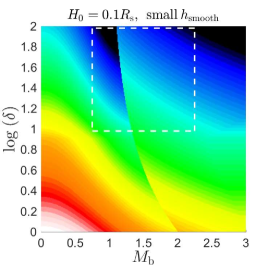
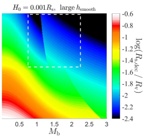
Figure 15: The critical stream radius for a factor 2 reduction in the inflow velocity of cold gas onto the central galaxy due to KHI, $R_{\rm s,dec}$, as a function of $M_{\rm b}$ and $\delta$. In the absence of the gravitational acceleration of the dark matter halo, streams with $R_{\rm s}<R_{\rm s,dec}$ are expected to decelerate to less than half their initial velocity in a virial crossing time. $R_{\rm s,dec}$ is given by either eq. (47) or eq. (48), depending on whether surface or body modes dominate the instability, as described in the text. The two panels represent the same two extreme limits as in Fig. 14 for the regime where body modes are unstable. By definition, these two limits have no effect at $M_{\rm b}<(1+\delta^{-1/2})$. At larger Mach numbers, the critical radii in the left-hand panel are only $\sim 40\%$ larger than those in the right-hand panel throughout the range of $(M_{\rm b},\delta)$ values relevant for cold streams, marked by dashed squares. $R_{\rm s,dec}$ ranges from $\sim(0.004-0.03)R_{\rm v}$, decreasing towards higher $\delta$ and higher $M_{\rm b}$, save for a jump to larger values when body modes destabilize. This is a factor of $3-4$ larger than the corresponding range of critical radii for disruption of 2d slabs.

5.3 Deceleration and Kinetic Energy Dissipation

The deceleration of stream fluid due to KHI is interpreted in the cosmological case as a reduction in the inflow rate of cold gas onto the central galaxy. As a crude estimate of the magnitude of this effect, following P18 we estimate the critical stream radius for a factor of 2 reduction in inflow rate to occur prior to reaching the central galaxy, $R_{\rm s,dec}$.

Surface modes reduce the stream velocity to half its initial value after a time $\sim\tau_{\rm surface,\,3d}$, which is proportional to $R_{\rm s}$ (eq. 12). By requiring that $\tau_{\rm surface,\,3d}=t_{\rm v}=R_{\rm v}/V_{\rm v}$, we obtain the critical stream radius

$$\frac{R_{\rm s,dec}^{\rm surface}}{R_{\rm v}}=\dfrac{\alpha_{\rm b}\sqrt{\delta}}{\left(1+\sqrt{\delta}\right)\left(\sqrt{1+\delta}-1\right)},$$ (47)

where $\alpha_{\rm b}$ represents shear layer penetration into the background rather than the stream. For $\delta<8$ we approximate $\alpha_{\rm b}$ with eq. (4) while for $\delta>8$ we use half of this value, in order to account for the decrease in the expansion rate of the shear layer into the background once $h_{\rm b}\sim(1.5-2)R_{\rm s}$, as explained in §4.1 and shown in Fig. 5. Our simulations show that this decreased value of $\alpha_{\rm b}$ reproduces stream deceleration rates at high $\delta$ (Fig. 9).

If the instability is initially dominated by body modes, the stream only begins to decelerate after the critical perturbation becomes nonlinear, at $t_{\rm NL}$ (eq. 16). From this point, the stream decelerates at a roughly constant rate until it reaches half its initial velocity. In §4.2 we showed that the timescale for the stream to reach half its initial velocity can either be expressed as $\sim 10\tau_{\rm body,\,3d}$ (eq. 20) or as $\tau_{\rm surface,\,3d}$ with $\alpha_{\rm b}=0.05$. These two timescales are very similar for values of $(M_{\rm b},\delta)$ typical of cold streams, while the former becomes smaller as either $M_{\rm b}$ or $\delta$ are increased. For the remainder of this analysis we adopt $\sim 10\tau_{\rm body,\,3d}$ as the relevant timescale, but stress that this choice has no significant effect on our conclusions. The resulting critical radius for deceleration due to body modes is

$$\frac{R_{\rm s,dec}^{\rm body}}{R_{\rm v}}=\left[10M_{\rm b}\left(\sqrt{1+\delta}-1\right)+M_{\rm b}\sqrt{\delta}~{}{\rm ln}\left(\dfrac{R_{\rm s}}{H_{0}}\right)\right]^{-1}.$$ (48)

Note that unlike eq. (47), this condition depends on the initial conditions through the initial amplitude of the critical perturbation, $H_{0}$.

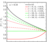
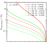
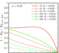
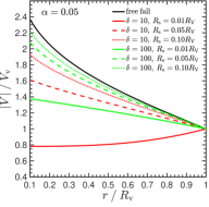
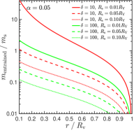
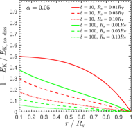
Figure 16: Evolution of a stream in the CGM of a massive dark matter halo, according to solutions of a toy model including gravitational acceleration and a friction-like deceleration due to KHI. eqs. (51)-(52). The horizontal axes show the halocentric radius normalized by the halo virial radius, and the vertical axes show the magnitude of the inflow velocity normalized to the halo virial velocity (left, with the black solid lines showing the free fall solution), the mass of backgroud gas entrained in the shear layer normalized by the stream mass (middle), and the fraction of bulk kinetic energy associated with laminar flow which is lost (right). In each panel, the red and green lines show solutions for $\delta=10$ and $100$ respectively, while the solid, dashed and dotted lines show solutions for $R_{\rm s}/R_{\rm v}=0.01$, $0.05$, and $0.10$ respectively. The top (bottom) row shows results assuming a constant value of $\alpha=0.1$ ($0.05$). Realistic stream values are likely bracketed by the solid and the dashed green lines and by these two values of $\alpha$ (see text). For these values, we see that KHI can significantly contribute to the deceleration of streams as they fall down the potential well of massive dark matter halos, while the mass entrained within the shear layer is a significant fraction of the stream mass, and can exceed it in some cases. Overall, $\sim 10-50\%$ of the bulk kinetic energy is lost to a combination of turbulence, thermal energy, and sound waves, and may subsequently be dissipated into radiation.

Figure 15 shows the resulting critical stream radius for a factor of 2 reduction in inflow velocity, $R_{\rm s,dec}/R_{\rm v}$, as a function of $M_{\rm b}$ and $\delta$. The two panels show the same two extreme limits for the body mode regime as in Fig. 14. As before, the behaviour at $M_{\rm tot}<1$ is identical in these two limits by definition. At larger Mach numbers, the critical radius in the former limit is only $\sim 40\%$ larger than in the latter limit throughout the parameter range relevant for cold streams, marked by a dashed square in each panels. We find that streams with radii up to $\sim 0.03R_{\rm v}$ can decelerate to half their initial velocity prior to reaching the galaxy due to KHI. The critical radius ranges from $R_{\rm s,dec}\sim(0.004-0.03)R_{\rm v}$, decreasing with $\delta$, and tending to decrease with $M_{\rm b}$ as well save for a jump to larger values when body modes destabilize. For 2d slabs, deceleration was found to be negligible, with the corresponding critical radius ranging from $R_{\rm s,dec}\sim(0.001-0.01)R_{\rm v}$ (P18), below the expected range of radii for cold streams (eq. 44). The 3d geometry thus increases the potential for stream deceleration by a factor of $\sim 3-4$.

The above discussion of stream deceleration ignores the gravitational acceleration due to the dark matter halo through which the stream is flowing. This can compensate for some or all of the deceleration caused by KHI, and may be related to the roughly constant inflow velocities of cold streams seen in cosmological simulations at much lower resolution (Dekel et al., 2009; Goerdt & Ceverino, 2015), where KHI is at best marginally resolved. In P18 we introduced a simple toy model to estimate the radial velocity profile of a stream in the CGM of a dark matter halo, finding that unless $\delta\sim 10$ and $R_{\rm s}/R_{\rm v}\sim 0.01$, which is an unlikely combination according to eq. (44), the stream velocity profile was very close to the free-fall velocity. We revisit this model below and apply it to 3d cylindrical streams rather than 2d slabs.

The stream fluid is modeled as a rigid body falling radially into the halo under the influence of gravity and a drag-like force associated with KHI. The dark matter halo is modeled as a singular isothermal sphere, with a mass profile $M(r)=V_{\rm v}^{2}r/G$, where $r$ is the halocentric radius, $G$ is Newton’s constant, and $V_{\rm v}={\rm const}$ is the halo virial velocity. The gravitational acceleration at radius $r$ is thus

$$a_{\rm g}=-\frac{V_{\rm v}^{2}}{r}.$$ (49)

We assume that within the halo the stream has a conical shape as it is focused towards the halo centre, so that its radius at halocentric distance $r$ is

$$r_{\rm s}(r)=\frac{R_{\rm s}}{R_{\rm v}}r.$$ (50)

This is consistent with cosmological simulations (Dekel et al., 2009; van de Voort & Schaye, 2012). We model the deceleration due to KHI, $\dot{V}_{\rm KHI}$, using eq. (37), which we found to be a good fit for both surface modes (Fig. 9) and body modes (Fig. 13). We replace the constant stream radius, $R_{\rm s}$, in eq. (37) with by $r_{\rm s}(r)$, and assume that the density contrast, $\delta$, is independent of radius.

Combining eqs. (37), (49) and (50), one obtains an equation of motion for the stream under the influence of gravity and KHI-induced drag. Since ${\rm d}V/{\rm d}t=0.5({\rm d}V^{2}/{\rm d}r)$, this can be converted into a differential equation for the radial velocity profile, $V(r)$, with the boundary condition $V(r=R_{\rm v})=V_{\rm v}$. The solution is

$$\frac{V(r)}{V_{\rm v}}=\left\{\begin{array}[]{c c}-\sqrt{\dfrac{(B-2)x^{B}+2}{B}}&B\neq 0\\ \\ -\sqrt{1-2{\rm ln}(x)}&B=0\end{array}\right.,$$ (51)

where $x=r/R_{\rm v}$, and

$$B=\frac{2\alpha\sqrt{\delta}R_{\rm v}}{(1+\sqrt{\delta})(\sqrt{1+\delta}-1)R_{\rm s}}.$$ (52)

The case $B=0$ represents gravitational free-fall, corresponding to $\alpha=0$.

In the left-hand panels of Fig. 16, we show the resulting radial profiles for $\delta=10,100$ and $R_{\rm s}/R_{\rm v}=0.01,0.05,0.10$, as well as for free-fall. The top (bottom) row shows the results for $\alpha=0.1~{}(0.05)$, which bracket the range of $\alpha$ values relevant for cold streams (Fig. 6). For narrow streams, with $R_{\rm s}/R_{\rm v}=0.01$, the deceleration due to KHI is able to overcome the gravitational acceleration. With $\alpha=0.1$, dense streams with $\delta=100$ maintain a constant inflow velocity throughout the halo, reaching $0.1R_{\rm v}$ with a velocity $\sim 0.42$ times the free-fall velocity, hereafter $V_{\rm ff}$. Dilute streams with $\delta=10$ actually net decelerate in the CGM, reaching $0.1R_{\rm v}$ at $\sim 0.55$ times their initial velocity, or $\sim 0.23V_{\rm ff}$. However, based on eq. (44) such a narrow and dilute stream is an unlikely combination, and furthermore would be expected to disrupt while still in the CGM (Fig. 14). Streams with $R_{\rm s}=0.05R_{\rm v}$, which are not likely to disrupt before reaching the central galaxy (Fig. 14), also show non-negligible deceleration, reaching $0.1R_{\rm v}$ with velocities $\sim 0.52V_{\rm ff}$ and $0.78V_{\rm ff}$ for $\delta=10$ and $100$ respectively. Even very wide streams, with $R_{\rm s}/R_{\rm v}=0.10$, reach $0.1R_{\rm v}$ with $\sim 0.68V_{\rm ff}$ for $\delta=10$. For $\delta=100$, the velocity is $\sim 0.88V_{\rm ff}$, though such wide and dense streams are unlikely based on eq. (44). Using $\alpha=0.05$ in eq. (52) increases the velocities at $0.1R_{\rm v}$ by $\sim(10-40)\%$ compared to $\alpha=0.1$. Overall, these results show that KHI can be significant in preventing the acceleration of streams as they fall down the potential well of dark matter halos, contrary to the results of the 2d analysis in P18, highlighting the importance of the 3d analysis presented here.

While our results suggest that KHI is unlikely to maintain a constant inflow velocity unless the streams are very narrow, $R_{\rm s}\sim 0.01R_{\rm v}$, in Appendix §B we found that in systems dominated by high-$m$ surface modes, the deceleration rates are overestimated in low resolution simulations. This may explain why cosmological simulations indicate constant velocities for streams which can be much wider than $0.01R_{\rm v}$.

We now extend the toy model beyond its original use in P18. In §4 we showed that stream deceleration can be described by a toy model where background mass is entrained in a shear layer, mixes with the original stream fluid and shares its initial momentum. As indicated by the total bulk kietic energy loss rates shown in Figs. 9 and 13, the simplifying assumption that the velocity within the shear layer is constant and equal to the stream velocity seems consistent with simulation results. We thus evaluate the accretion rate of background fluid into the shear layer using eq. (39) with $\dot{v}$ representing only KHI induced deceleration, $\dot{V}_{\rm KHI}$, without $a_{\rm g}$ from eq. (49). Using $\dot{m}=V{\rm d}m/{\rm d}r$, and the boundary condition $m_{\rm entrained}(r=R_{\rm v})=0$, we obtain

$$\frac{m_{\rm entrained}}{m_{\rm s}}=x^{-B/2}-1,$$ (53)

where $m_{\rm entrained}$ is the total background mass entrained in the shear layer and $m_{\rm s}$ is the initial stream mass. As in eq. (51), $x=r/R_{\rm v}$ and $B$ is given by eq. (52). This is shown in the centre panels of Fig. 16. In most cases the entrained mass at $0.1R_{\rm v}$ is a significant fraction of the stream mass, and for narrow streams, $R_{\rm s}\lower 2.58333pt\hbox{$\;\buildrel<\over{\sim}\;$}0.03R_{\rm v}$, the entrained mass can significantly outweigh the initial stream even for density contrasts of $\delta=100$. For $\delta=10$, the entrained mass equals the initial stream mass for stream radii $R_{\rm s}\sim(0.05-0.1)R_{\rm v}$ for $\alpha\sim(0.05-0.1)$. For $\delta=100$, this occurs at $R_{\rm s}\sim(0.02-0.03)R_{\rm v}$. Only for very dense and wide streams, which are unlikely based on eq. (44), does the entrained mass amount to only a small fraction, $\sim 10-20\%$, of the stream mass.

Combining eqs. (51) and (53), we can estimate the kinetic energy of the inflowing material as $E_{\rm K}\sim 0.5(m_{\rm entrained}+m_{\rm s})V^{2}$, where as in eqs. (39) and (40) we have assumed that the entrained material and the stream material are fully mixed and moving at the same velocity, which seems consistent with simulations as shown in §4. We wish to compare this to the total kinetic energy the system would have were there no deceleration. However, this is not simply $0.5m_{\rm s}V_{\rm ff}^{2}$, since by virtue of adding additional mass to the system and transporting it down the potential well, gravity is doing more work than it would have on the stream alone, and this must be accounted for when estimating the energy dissipation. In fact, since the entrained mass is such a large fraction of the stream mass and can even exceed it, the kinetic energy of the system can actually be larger than $0.5m_{\rm s}V_{\rm ff}^{2}$ even after energy losses. We will comment further on the physical implications of this below. The total kinetic energy of the system without any deceleration is given by

$$\begin{array}[]{c}E_{\rm K,\,no\>diss}(r)=\dfrac{m_{\rm s}V_{\rm ff}^{2}(r)}{2}\\ +\displaystyle\int_{r}^{R_{\rm v}}\dfrac{{\rm d}m_{\rm entrained}}{{\rm d}\tilde{r}}[\Phi(r)-\Phi(\tilde{r})]~{}{\rm d\tilde{r}},\end{array}$$ (54)

where $\Phi(r)=-V_{\rm v}^{2}[{\rm ln}(r/R_{\rm v})-1]$ is the potential of a singular isothermal sphere truncated at $R_{\rm v}$. The result is

$$E_{\rm K,\,no\>diss}(x)=\frac{m_{\rm s}V_{\rm ff}^{2}(x)}{2}\left[1+\frac{4\left(x^{-B/2}-1\right)}{B}\right].$$ (55)

In the right-hand panels of Fig. 16 we show the dissipation of bulk kinetic energy due to KHI, $1-E_{\rm K}/E_{\rm K,\,no\>diss}$. With the exception of the case $\delta=10,R_{\rm s}/R_{\rm v}=0.01$, which entrains many times its own mass, all cases very nearly have $E_{\rm K}/E_{\rm K,\,no\>diss}\sim V/V_{\rm ff}$, in agreement with eq. (40), showing the consistancy of our model. Ignoring the cases $\delta=10,R_{\rm s}/R_{\rm v}=0.01$ and $\delta=100,R_{\rm s}/R_{\rm v}=0.10$ which are unlikely based on eq. (44), we see that when the stream reaches $0.1R_{\rm v}$ between $10-40\%$ of the kinetic energy is lost for $\alpha=0.05$ and between $20-50\%$ for $\alpha=0.1$. As described in §4.1, the lost kinetic energy is split between turbulent energy, thermal energy of either the stream or the background, and sound waves propagating away from the stream, and as such represents an upper limit to the amount of energy which will eventually be dissipated into radiation.

It has been suggested that the observed Lyman-$\alpha$ blobs (LABs), with luminosities of $10^{42}-10^{44}~{}{\rm erg\,s^{-1}}$ around halos with masses of $M_{\rm v}\sim 10^{11}-10^{13}$ at $z=3$, can be powered by the dissipation of gravitational energy in cold streams feeding these galaxies, provided the fraction of energy radiated away exceeds $\sim 20\%$ (Dijkstra & Loeb, 2009). Similar conclusions were reached by Goerdt et al. (2010) based on cosmological simulations (though see also Faucher-Giguère et al., 2010 for a less optimistic view). Based on this, we conclude that KHI can contribute significantly to the observed Lyman-$\alpha$ luminosity of LABs. We stress that this is contrary to the conclusions reached following the 2d analysis in P18, highlighting the importance of our current analysis. A potential caveat to this conclusion is that while the bulk of the stream may be self-shielded to the UVB (Goerdt et al., 2010; Faucher-Giguère et al., 2010), this may not be true for the shear layer where the background fluid is entrained, which in turn may inhibit the production of Ly-$\alpha$ radiation. This will be studied in detail in an upcoming paper (Mandelker et al., in prep.), where we will include explicit radiative cooling in our calculations.

In our model, stream deceleration and energy dissipation are caused by background material, i.e. hot gas in the CGM, being entrained in and mixing with the stream, and eventually flowing toward the centre at the same velocity as the cold gas. Implicit in this is the assumption that the entrained gas is no longer held in hydrostatic equilibrium within the CGM. One likely expanation for this is the ram pressure of the cold gas. Cleary, in the unmixed stream core the ram pressure is significantly larger than the thermal pressure of the hot gas, since $M_{\rm b}\sim 1$ and $\delta>>1$, and even in the shear layer the ram pressure can still be larger than the thermal pressure. This will be studied in more detail in future work which explicitly accounts for the external halo potential. An additional intriguing possibility is the presence of thermal instabilities in the shear layer which may cause the hot gas to cool and condense onto the cold stream. This issue will be further studied in detail in and upcoming paper (Mandelker et al., in prep.), where we will examine the nonlinear evolution of KHI with radiative cooling. If this indeed occurs, the cooling radiation of the entrained gas as it mixes with the stream could be another powerful source of radiation not considered in our current work.

6 Additional Physics and Future Work

While the analysis presented here has been thorough and exhaustive in terms of adiabatic hydrodynamics, it is worth noting potential caveats to our conclusions due to additional physics not included in our current analysis. The detailed effects of these processes on the stability of cold streams feeding massive galaxies at high redshift will be the subject of future work, where we will add them one by one to our current framework.

We begin by considering radiative cooling, which is clearly very important for the evolution of cold streams. Previous studies have found that radiative cooling can either enhance or suppress the growth rates of KHI in the linear regime, depending on the slope of the cooling function and on the ratio of the cooling time in each fluid to the sound crossing time (Massaglia et al., 1992; Bodo et al., 1993; Vietri, Ferrara & Miniati, 1997; Hardee & Stone, 1997; Xu, Hardee & Stone, 2000). In our case, the cooling time in the hot halo is typically much longer than the stream sound crossing time, while the cooling time in the streams is typically much shorter. Under these conditions, the linear growth rates at wavelengths $\lambda\lower 2.58333pt\hbox{$\;\buildrel>\over{\sim}\;$}R_{\rm s}$ are very similar to the adiabatic case considered here (Mandelker et al., in prep.). However, radiative cooling can substantially alter the nonlinear evolution of KHI in dense streams (Vietri, Ferrara & Miniati, 1997; Stone, Xu & Hardee, 1997; Xu, Hardee & Stone, 2000; Micono et al., 2000), though the net effect again depends on the details of the cooling function and the stream parameters. Some authors find that radiative cooling leads to more violent disruption of the stream (Stone, Xu & Hardee, 1997; Xu, Hardee & Stone, 2000), while others find that cooling prevents stream disruption by limiting the penetration of the shear layer into the stream (Vietri, Ferrara & Miniati, 1997; Micono et al., 2000), though the deceleration rates remain similar to the adiabatic case (Micono et al., 2000). It is also found that KHI in a cooling medium leads to much larger density fluctuations, and to the formation of dense knots and filaments inside the stream. In an upcoming paper (Mandelker et al., in prep.) we will examine the nonlinear evolution of KHI with radiative cooling for parameters typical of cold streams. Preliminary results suggest that the stream remains more colimated and denser, and is less prone to dissintegarion, though the deceleration rates are slightly larger than in the adiabatic case.

The self-gravity of the gas streams may also affect their evolution. It has been suggested that for a wide range of typical parameters cold streams are gravitationally unstable, as their mass per unit length, $M_{\rm L}\simeq\pi R_{\rm s}^{2}\rho_{\rm s}$, is larger than the critical mass for filament stability (Mandelker et al., 2018). This can lead to stream fragmentation in the halo irrespective of KHI, which would completely alter our analysis. Density fluctuations induced by KHI may also trigger local collapse before the entire stream has fragmented. On the other hand, if the streams are marginally gravitationally stable, the self-gravity can stabilize the KHI and prevent stream disruption. This has been demonstrated in the context of cold, dense, spherical clouds moving through a hot medium, meant to represent giant molecular clouds moving through the interstellar medium (Murray et al., 1993). In an upcoming paper (Aung et al., in prep) we will examine the evolution KHI in cold streams with self-gravity. Preliminary results suggest that so long as the stream is globally gravitationally stable, self-gravity suppresses stream disruption though has only a small effect on stream deceleration. Furthermore, the gravitational potential of the host dark matter filament can affect the gravitational stability of the stream. It may stabilize the stream by making it more buoyant, or it may destabilize the stream by increasing the inward radial gravitational force, thus requiring non-thermal turbulent motions to support the stream against radial collapse. These issues will be explored in future work.

The central gravity of the dark matter halo into which the streams are flowing may also affect their evolution. In §5.3 we attempted to estimate the net deceleration of streams falling down the potential well of a dark matter halo while undergoing KHI. While we showed that non-negligible net deceleration may still occur, this model was very simplistic and a more detailed study is warranted. Furthermore, as the stream is focused towards the centre of the potential it assumes a roughly conical shape, with its radius decreasing towards the halo centre (Dekel et al., 2009; van de Voort & Schaye, 2012). As narrower streams disrupt faster (Fig. 14), this can greatly enhance the potential for stream disruption in the CGM. These issues will be the focus of future work.

As noted in §5.2, thermal conduction will set the scale of the transition region between the stream and the background, which can greatly influence the stability of short wavelength perturbations and high-$m$ surface modes. While this has been qualitatively accounted for in our current analysis, it is unclear whether thermal conduction may further alter the evolution of the instability, especially when cooling is included. This is further complicated by the fact that the conduction length in the hot halo is likely orders of magnitude larger than in the cold stream (M16). Finally, magnetic fields parallel to the flow have been found to stabilize high-$m$ modes due to an effective surface-tension which suppresses the presence of small scale structure on the stream boundary (Ferrari, Trussoni & Zaninetti, 1981; Birkinshaw, 1990). However, in the high redshift streams we are considering, the magnetic field is expected to be very weak, with the plasma beta parameter possibly as large $\beta\lower 2.58333pt\hbox{$\;\buildrel>\over{\sim}\;$}1000$ (M16). We therefore do not expect magnetic fields to fundamentally alter our conclusions. However, even a dynamically unimportant magnetic field can significantly weaken thermal conductivity and viscosity, so it will be important to account for these effects simultaneously in future work.

Finally, we speculate that the spectrum and amplitude of initial perturbations in the stream will be determined primarily by the cosmological context, such as a non-trivial accretion geometry and non-zero impact parameter with respect to the central galaxy, deviations from pressure equilibrium as the stream enters the virial shock, galactic or AGN feedback, turbulence in the halo, etc. To study this, efforts are underway to perform fully cosmological simulations with tailored refinement along streams in order to properly resolve their structure and stability (Cornuault et al., in prep). In this context, cosmological simulations without star-formation and feedback may also be employed to study the effects of accretion geometry and entry into the shock region.

7 Summary and Conclusions

Massive star-forming galaxies (SFGs) at redshifts $z\lower 2.58333pt\hbox{$\;\buildrel>\over{\sim}\;$}1$ are thought to be fed by cold streams ($T\sim 10^{4}\,{\rm K}$) of dense gas that flow along cosmic web filaments, through the hot circumgalactic medium (CGM) containing dilute gas at the virial temperature ($T\sim 10^{6}\,{\rm K}$). These streams have Mach numbers of $M_{\rm b}\sim 0.75-2.25$ with respect to the sound speed of the hot halo, density contrasts of $\delta\sim 10-100$ compared to the hot halo, and radii of $R_{\rm s}\sim 0.01-0.10$ times the halo virial radius. While this is yet to be confirmed observationally, it is a robust theoretical concept, and is seen in numerous different cosmological simulations (Kereš et al., 2005; Dekel & Birnboim, 2006; Ocvirk, Pichon & Teyssier, 2008; Dekel et al., 2009; Ceverino, Dekel & Bournaud, 2010; Faucher-Giguère, Kereš & Ma, 2011; van de Voort et al., 2011). In order to study the evolution of these streams as they travel through the CGM towards the central galaxy, we presented here a detailed study of the nonlinear stage of purely-hydrodynamic, adiabatic Kelvin-Helmholtz Instability (KHI) in 3d cylinders, using both analytic models and RAMSES numerical simulations. This extended our previous work on the linear phases of the instability (Mandelker et al., 2016), and the nonlinear instability in 2d planar slabs (Padnos et al., 2018). Our main results from this paper can be summarized as follows.

1. For streams which are subsonic with respect to the sum of the two sound speeds, i.e. $M_{\rm tot}<1$ (eq. 2), the instability is dominated by surface modes, and the nonlinear evolution of 3d cylinders is qualitatively similar to 2d slabs. It is driven by vortex mergers that lead to self-similar shear layer growth in a ring-like structure around the stream. The shear layer growth rate, the convection (drift) velocity of the largest eddies along the stream, and the ratio of shear layer thickness in the stream/background are all very similar in 2d slabs and 3d cylinders, and follow our analytic predictions. However, the timescale for the shear layer to encompases the entire stream width is roughly $\sim 0.5$ as long in 3d as it is in 2d. Furthermore, 3d cylinders decelerate significantly faster than 2d slabs, by up to a factor of $\sim 10$ for density contrasts of order $100$. This is because the shear layer expanding into the background fluid sweeps up mass at a higher rate. Overall, as either the density contrast between the stream and background, $\delta$, or the Mach number of the stream with respect to the background sound speed, $M_{\rm b}$, are increased, the shear layer growth rates decreases, the ratio of shear layer thickness in the two fluids diverges from unity, and the deceleration rates decrease.

2. For 3d cylindrical streams with $M_{\rm tot}<1$, once the shear layer has expanded to roughly $2R_{\rm s}$ the largest eddies begin to break up and cascade towards smaller scales. This drives turbulence and enhances mixing of the stream and background fluids, while at the same time decreasing both the expansion rate of the shear layer and the deceleration rate of the stream. This drives turbulence, enhances mixing of the stream and background fluids, and slows the growth of the shear layer. The turbulence in the shear layer reaches a maximal value of $\sigma/V\sim(0.2-0.3$) and then decays to an assymptotic value of $\sim(0.1-0.2)$, independent of $M_{\rm b}$ or $\delta$, where $V$ is the initial velocity of the stream. At late times, $\sim 10\%$ of the initial bulk kinetic energy is in turbulent motions of both stream and background fluid, and on scales $\lower 2.58333pt\hbox{$\;\buildrel<\over{\sim}\;$}R_{\rm s}$ the turbulence is roughly isotropic. This is unlike the situation in 2d where the largest eddies do not break up, the shear layer continues to expand by mergers of larger and larger eddies, and the magnitude of turbulence is not universal.

3. For streams which are supersonic with respect to the sum of the two sound speeds, i.e. $M_{\rm tot}>1$, there is a qualitative difference between 2d slabs and 3d cylinders. In 2d geometry, surface modes have completely stabilized, while 3d cylinders can still be unstable to azimuthal surface modes, characterized by a mode number, $m$, and associated azimuthal wavelength, $2\pi R_{\rm s}/m$. Such modes are unstable above a critical mode number, $m>m_{\rm crit}$ (eq. 13), which depends on $M_{\rm b}$, $\delta$, and the longitudinal wavelength of the perturbation, with shorter wavelengths having larger $m_{\rm crit}$. However, the $m$-th mode is only unstable provided the initial transition region between the pure stream and background fluids is narrower than $2\pi R_{\rm s}/m$. These modes behave very similarly to the “standard” surface modes described above, and their nonliner growth is dominated by self-similar shear layer growth. However, the largest eddies are smaller, $\propto m^{-1}$, rendering the turbulent cascade difficult to resolve. Low resolution simulations in this regime thus overestimate both shear layer growth and stream deceleration (appendix §B).

4. If the width of the initial transition region between the stream and background is large enough, high-$m$ surface modes are stable. For streams with $M_{\rm tot}>1$, the instability will thus be dominated by body modes, as in the 2d case. The nonlinear evolution of body modes is driven by long-wavelength sinusoidal perturbations. We find good agreement between the analytical predictions for the critical perturbation mode that is expected to break the stream, and the dominant mode observed at late times in numerical simulations. While these are similar for 2d slabs and 3d cylinders, the timescale for this perturbation to become nonlinear is $\sim 0.5$ as long in 3d as it is in 2d (Table 1). Unlike for surface modes, the timescales for nonlinear evolution of body modes explicitly depend on the initial conditions through the initial amplitude of the long-wavelength critical perturbation. Once this perturbation becomes non-linear, a higly turbulent structure rapidly develops, similar to subsonic streams, encompasing the entire stream and mixing it with the background within roughly one sound crossing time. This is contrary to the evolution in 2d slabs, where the slab expands to $\sim 8-10$ times its initial width and breaks up into discrete blobs which remain unmixed for several sound crossing times. Similar to surface modes in subsonic streams, body modes in supersonic streams also lead to much faster deceleration in 3d compared to 2d, due to similar geometrical effects.

5. We predict that for a significant region of the allowed parameter range, KHI can cause cold streams feeding massive galaxies at high redshfit to disintegrate prior to reaching the central galaxy. The upper limit for the stream radius that results in disintegration depends on the Mach number, the density contrast, the initial amplitude of the critical body-mode perturbation, and the initial width of the transition region between the stream and the background. For typical parameters, this critical radius ranges from $\sim(0.005-0.05)R_{\rm v}$, roughly $70\%$ larger than the critical radius deduced for 2d slabs.

6. Unlike 2d slabs, where KHI was found to have little to no impact on the stream velocities in the CGM, for 3d cylinders KHI can cause significant stream deceleration before they reach the central galaxy. The upper limit for the stream radius that results in a factor of $\geq 2$ decrease in the inflow velocity ranges from $\sim(0.004-0.03)R_{\rm v}$, a factor of $\sim 4$ larger than the critical radius for 2d slabs. Furthermore, using a simple toy model to estimate the balance between the gravitational acceleration towards the halo centre and the deceleration induced by KHI in the CGM, we estimate that the inflow velocities of streams can be significantly less than the free-fall velocity. Since the deceleration is overestimated in low resolution simulations where high-$m$ surface modes dominate, (appendix §B), this may explain the roughly constant inflow velocities of streams seen in cosmological simulations.

7. Using a simple toy model to estimate the loss of bulk kinetic energy assocaited with laminar flow of both the stream and background fluids induced by KHI in the CGM, we estimate that typical streams can loose up to $\sim(10-50)\%$ of the gravitational energy gained between $R_{\rm v}$ and $0.1R_{\rm v}$. This suggests that KHI can be a viable power source for the observed emission of Lyman-$\alpha$ blobs. However, this is only an upper limit on the total amount of energy which will actually be radiated away, as some of it can go into sound waves which escape the system, or into thermal energy of the hot medium. This will be explored in detail in future work which will incorporate radiative cooling (Mandelker et al., in prep.).

8. Potential caveats to our results stem from the lack of important physical processes beyond adiabatic hydrodynamics, such as radiative cooling, the self-gravity of the stream, the external gravity of the halo, magnetic fields and thermal conduction. It is very likely that these will have a significant impact on the stream morphology and eventual disruption, though we speculate that our results regarding stream deceleration may not change as significantly. In ongoing and future work, we will explicitly account for these processes and more accurately address the evolution and fate of cold streams in massive, hot halos.

Appendix A Simulating the linear regime

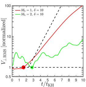
Figure 17: Perturbaion amplitude as a function of time in the linear regime. Shown are results for two simulations, $(M_{\rm b},\delta)=(1,10)$ in red and $(2,10)$ in green. Each simulation was initiated with a single wavelength ($\lambda=R_{\rm s}$), helical ($m=1$), perturbation in the radial velocity, as described in the text. The time in each panel has been normalized by the KH time of the fastest growing eigenmode, and the perturbation amplitude is estimated by the RMS of the transverse velocity. Perturbations must evolve into eigenmodes before they can grow. For surface modes, as in the $M_{\rm b}=1$ case, the timescale for this is the perturbation sound crossing time, $t_{\rm\lambda}=\lambda/c_{\rm b}$, marked with a red circle. For body modes, as in the $M_{\rm b}=2$ case, it is the stream sound crossing time, $t_{\rm sc}$, marked with a green star. The perturbation amplitude have been normalized to unity at these times. The slope of the dashed line marks the expected exponential growth at later times (the zero-point has been shifted for clarity). The $M_{\rm b}=1$ simulation shows a good match to the analytic prediction, underestimating the growth rate by less than $20\%$, due to the smoothing in the initial conditions. The growth in the $M_{\rm b}=2$ case is oscillatory, due to the large smoothing in the unperturbed solution and to mode interactions, though during periods of growth the slope is a good match to the analytic prediction.

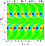
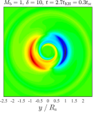
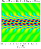
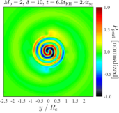
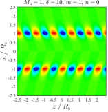
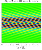
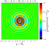
Figure 18: Development of eigenmodes in simulations with a single wavelength perturbation. The top row shows the pressure perturbation for the same two simulations as in Fig. 17. The left two panels are for the $M_{\rm b}=1$ case, while the right two panels are for the $M_{\rm b}=2$ case. For each simulation we show both a slice through the $zy$ plane (1st and 3rd panels), and a slice through the $xy$ plane (2nd and 4th panels). The simulations are shown shortly after the fastest growing eigenmode has developed and begun to grow, $t\sim 0.3t_{\rm sc}$ for $M_{\rm b}=1$ and $t\sim 2.4t_{\rm sc}$ for $M_{\rm b}=2$. The bottom row shows the predicted pressure distribution for the eigenmodes whose growth rates were used in Fig. 17. The resemblance of the simulated perturbation to the analytic mode is striking, showing that our simulations properly capture the linear evolution.

In this section we present simulations of the linear evolution of single wavelength perturbations in 3d cylinders. This serves both to test the numerical scheme we use throughout the paper, as well as to test the analytic predictions for the growth rate and eigenmode structure of linear perturbations in 3d cylinders presented in M16 (section 2.4).

We perform two simulations, with $(M_{\rm b},\delta)=(1,10),$ and $(2,10)$, meant to represent surface and body modes, respectively. The unperturbed initial conditions were set up as described in §3.2. For the simulation with $M_{\rm b}=1$ we used $\sigma=R_{\rm s}/32$ in eq. (23), as in the surface-mode simulations presented in §4.1. For the $M_{\rm b}=2$ case we used $\sigma=R_{\rm s}/8$, as in the body-mode simulations presented in §4.2. In both simulations, we initiate a perturbation in the radial component of the velocity, following eqs. (24)-(25), with a single wavelength, $\lambda=R_{\rm s}$ so $k=2\pi/R_{\rm s}$, and helical symmetry, $m=1$. The perturbation amplitude is $0.01c_{\rm s}$ as in our main analysis. For the $M_{\rm b}=1$ case we set $\sigma_{\rm pert}=R_{\rm s}/16$, while for $M_{\rm b}=2$ we use $\sigma_{\rm pert}=R_{\rm s}/8$, as for the simulations in §4.1 and §4.2 respectively.

Figure 17 shows the perturbation amplitude as a function of time, normalized by the respective value of $t_{\rm KH}$ for the fastest growing mode in each simulation. For $M_{\rm b}=1$ this is the only available mode, the $n=0$ surface mode. For $M_{\rm b}=2$ this is the $n=2$ body mode (see M16 for details). The perturbation amplitude is estimated by the root-mean-squared (RMS) value of the transverse velocity, $v_{\perp}=(v_{\rm x}^{2}+v_{\rm y}^{2})^{1/2}$. Before the perturbation can grow, it must evolve into an eigenmode of the system. For surface modes, the timescale over which this occurs is the sound crossing time of the perturbation in the hot medium, $t_{\rm\lambda}=\lambda/c_{\rm b}$, while for body modes it is the stream sound crossing time, $t_{\rm sc}$ (M16, section 3.3). In Fig. 17 we have normalized the perturbation amplitudes to unity at these times. Prior to this time the amplitude is not expected to grow appreciably, while afterwards it grows as ${\rm exp}(t/t_{\rm KH})$. The $M_{\rm b}=1$ simulation shows a good match to the analytic prediction, underestimating the growth rate by less than $20\%$, due to the smoothing in the initial conditions. The growth in the $M_{\rm b}=2$ case is oscillatory, likely due to the large smoothing in the unperturbed solution and to mode interactions, though during periods of growth the slope is a good match to the analytic prediction. Note that similar behavior was seen when examining the linear growth of body modes in 2d slab simulations (M16, figure 9).

The top row of Fig. 18 shows the spatial form of the pressure perturbation in each simulation shortly after the fastest growing eigenmode has developed, $t\sim 2.7t_{\rm KH}\sim 0.3t_{\rm sc}$ for $M_{\rm b}=1$ and $t\sim 6.9t_{\rm KH}\sim 2.5t_{\rm sc}$ for $M_{\rm b}=2$. For each simulation we show both an edge-on view (a slice in the $zy$ plane) and a face-on view (a slice in the $xy$ plane). The bottom row shows the analytic distribution of the pressure perturbation for the fastest growing eigenmode, computed following the procedure in section 2.4 of M16. The resemblance of the simulation results and the analytic prediction is striking, illustrating that the initial perturbation has evolved into eigenmodes and is dominated by the fastest growing mode. We conclude that our numerical scheme captures the linear evolution of the perturbations well.

Appendix B Convergence tests

In this section we test convergence of our results to the number of cells per stream radius, the refinement structure of the grid, and the random seed used to generate the initial conditions. We also discuss how convergence may depend on the width of the smoothing layer between the stream and the background and on the dominant unstable mode. This section refers only to 3d cylinders, as the convergence of 2d slab simulations was discussed in P18.

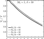
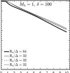
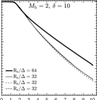
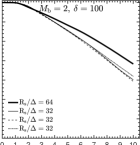
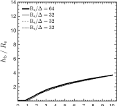
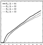
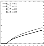
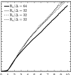
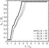
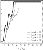
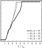
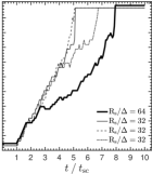
Figure 19: Convergence of our results with resolution, and variability introduced by the random seed. We compare results of our fiducial simulations with 128 cells per stream diameter (thick solid lines), to simulations with 64 cells per diameter (thin solid, dashed, and dot-dashed lines) run with three different random realizations of the perturbation phases (the thin solid line represents the same phases as the thick solid line). All other numerical parameters have their fiducial values described in §3. We show the stream deceleration, $V_{\rm s}/V$ (top), and the shear layer growth into the background, $h_{\rm b}$ (middle), and into the stream, $h_{\rm s}$ (bottom). The left-two columns show surface mode simulations with $M_{\rm b}<M_{\rm crit}$ while the right-two columns show simulations with $M_{\rm b}>M_{\rm crit}$. In all cases, the variability associated with the random seed is extremely small. The largest variability is in the time when the shear layer consumes the entire stream, $h_{\rm s}=R_{\rm s}$, as this is the most stochastic process. However, even here the variability about the mean is $\lower 2.58333pt\hbox{$\;\buildrel<\over{\sim}\;$}20\%$ in all cases. Surface mode simulations are converged at half our fiducial resolution. On the other hand, low resolution simulations with $M_{\rm b}>M_{\rm crit}$ are characterised by more rapid shear layer growth at $t\lower 2.58333pt\hbox{$\;\buildrel>\over{\sim}\;$}3t_{\rm sc}$ when $h_{\rm b}\lower 2.58333pt\hbox{$\;\buildrel>\over{\sim}\;$}2R_{\rm s}$, resulting in more rapid stream deceleration. This is due to the instability being dominated by high-order azimuthal surface modes, with azimuthal mode number $m\sim 12$ (Fig. 10). This leads to small initial eddies whose cascade to even smaller scales is unresolved, yielding more rapid shear layer growth as this process is dominated by the largest eddies. For high $M_{\rm b}$ simulations to converge, we require either higher resolution or a suppression of the high-$m$ modes.

B.1 Low Resolution and Random Seed

Figure 19 compares results of simulations with our fiducial resolution of 128 cells per stream diameter, $\Delta=R_{\rm s}/64$, to simulations at half the resolution, $\Delta=R_{\rm s}/32$. Furthermore, for the low resolution simulations we present results from three runs initiated with different random seeds. All runs were performed with our fiducial refinement strategy (§3.4) and fiducial smoothing of the initial conditions (§3.2, $\sigma=R_{\rm s}/32$ in eq. 23). We show results for $(M_{\rm b},\delta)=(1,10)$, $(1,100)$, $(2,10)$, and $(2,100)$. The first two have $M_{\rm b}<M_{\rm crit}$ (eq. 1) and are representative of the simulations presented in §4.1, while the latter two have $M_{\rm b}>M_{\rm crit}$ and are representative of the simulations presented in §4.2. For each simulation we show the stream deceleration (top, computed as in Fig. 9) and the growth of the shearing layer into the background (middle) and the stream (bottom, computed as in Fig. 5).

In all cases, the scatter induced by varying the random seed in very small, much smaller than the scatter induced in 2d slab simulations shown in P18. The smaller scatter likely results from the presence of many more eddies in 3d simulations than in 2d simulations due to the larger interface surface, resulting in less overall variability in the average merger times of eddies. Furthermore, the presence of a direct cascade in 3d simulations leading to small scale turbulence reduces the macroscopic variability further. The largest variability is in the final dissintegration of the stream by the shearing layer, i.e. the time when $h_{\rm s}=R_{\rm s}$. This is the most stochastic process, depending sensitively on when the largest eddies reach the stream axis. However, even here the scatter is less then $20\%$ about the mean.

The low $M_{\rm b}$ runs appear converged already at half our fiducial resolution. Stream deceleration and shear layer growth remain effectively identical at low resolution, modulo the aforementioned variability in the final stages of stream disruption. There is a slight systematic trend of shear layer growth begining slightly later in the low resolution simulations, by $<20\%$, resulting in a corresponding delay in the onset of deceleration. This is likely simply a result of the larger cell sizes requiring the interface to travel a larger distance before mixing is detected. Regardless, this has no effect on the rates of these processes.

The behaviour of the high $M_{\rm b}$ simulations is qualitatively different. At early times, the low resolution simulations behave identically to the fiducial runs. However, at $t\lower 2.58333pt\hbox{$\;\buildrel>\over{\sim}\;$}3t_{\rm sc}$, when $h_{\rm b}\lower 2.58333pt\hbox{$\;\buildrel>\over{\sim}\;$}2R_{\rm s}$, the growth rate of the shear layer becomes shallower in the fiducial runs than in the low resolution runs. This leads to a decrease in the deceleration rate, so the low resolution runs loose significantly more momentum by the end of the simulation. To explain these trends, we recall that these simulations are dominated by high-order azimuthal surface modes, with azimuthal mode number $m\sim 12$ (Fig. 10). As explained in §4.1, the shear layer growth rate of surface modes in 3d cylinders decreases once $h_{\rm b}\lower 2.58333pt\hbox{$\;\buildrel>\over{\sim}\;$}2R_{\rm s}$, since the energy cascade towards small scales results in less power at large scales to drive the growth. As the azimuthal mode number increases, the typical eddies become smaller and this cascade becomes harder to resolve. Thus, while it is converged for $m\sim 1$, it has not converged for $m\sim 12$, yielding a more rapid shear layer growth and stream deceleration as observed. We conclude that in order to properly resolve the late time behaviour of high-Mach number simulations, we must either go to higher resolution or else suppress the very high-$m$ modes. This is shown below.

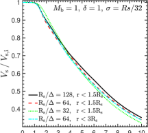
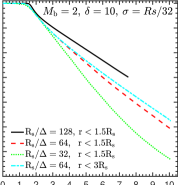
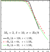
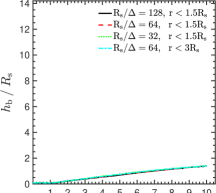
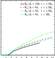
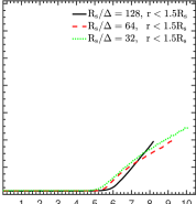
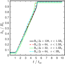
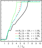
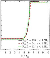
Figure 20: Convergence of our results with resolution, and with the refinement scheme. We compare results of our fiducial simulations with 128 cells across the stream diameter and cell sizes increasing by a factor of 2 every $3R_{\rm s}$ in the $x$ and $y$-directions (red dashed lines, dubbed $r<3R_{\rm s}$ in the legend), to simulations with the same resolution but where the cell size is increased every $1.5R_{\rm s}$ in the $x$ and $y$-directions (cyan dash-dotted lines, dubbed $r<1.5R_{\rm s}$ in the legend). We also compare simulations at half and double the fiducial resolution with the $r<1.5R_{\rm s}$ refinement. As in Fig. 19, we show the stream deceleration, $V_{\rm s}/V$ (top), and the shear layer growth into the background, $h_{\rm b}$ (middle), and into the stream, $h_{\rm s}$ (bottom). We show a surface mode simulation with $(M_{\rm b},\delta)=(1,1)$ on the left, and a body mode simulation with $(M_{\rm b},\delta)=(2,10)$ in the middle and right columns. The middle column shows a case with narrow smoothing, $\sigma=R_{\rm s}/32$, as in Fig. 19 so surface modes with $m\sim 12$ are unstable. The right-hand column shows a case with wide smoothing, $\sigma=R_{\rm s}/8$, so that modes with $m>4$ are stable. Note that this case does not show a simulation with the fiduial, $r<3R_{\rm s}$ refinement. In all cases shown, the difference between the two refinement schemes is extremely small, and we conclude that our results are converged with respect to this choice. The $(M_{\rm b},\delta)=(1,1)$ case is converged with resolution at half our fiducial value, as inferred from Fig. 19. The $(M_{\rm b},\delta)=(2,10)$ case with $\sigma=R_{\rm s}/32$ has not converged even at double our fiducial resolution. As inferred from Fig. 19, higher resolution runs evolve slower since they better resolve the breakup of the largest eddies of the $m\sim 12$ mode to smaller scales, leaving less power at large scales to drive the shear layer growth. However, when $\sigma=R_{\rm s}/8$, the $(M_{\rm b},\delta)=(2,10)$ case has converged even at half our fiducial resolution. In this case, the instability is dominated by larger structures which are better resolved, associated with an $m=1$ body mode and an $m=4$ surface mode. We conclude that for body mode simulations, convergence can be acchieved by suppressing the growth of high-order azimuthal modes.

B.2 High Resolution and Refinement Scheme

Figure 20 compares results of simulations with our fiducial resolution of 128 cells per stream diameter, $\Delta=R_{\rm s}/64$, to simulations with both half and double the resolution, $\Delta=R_{\rm s}/32$ and $R_{\rm s}/128$. For the fiducial resolution case, we also explore the effect of changing our refinement scheme from doubling the cell size every $3R_{\rm s}$ in the $x$ and $y-$directions to doubling the cell size every $1.5R_{\rm s}$. We show results for $(M_{\rm b},\delta)=(1,1)$ and $(2,10)$, each with our fiducial smoothing of $\sigma=R_{\rm s}/32$ in eq. (23), and also for $(M_{\rm b},\delta)=(2,10)$ with wider smoothing of $\sigma=R_{\rm s}/8$ as used in §4.2. As in Fig. 19, we show the stream deceleration (top), and the shear layer growth in the background (middle) and the stream (bottom).

In all cases, changing the refinement scheme has no affect on our results, as can be seen by comparing the red dashed lines to the cyan dot-dashed lines. The case $(M_{\rm b},\delta)=(1,1)$ is converged. While the shear layer begins growing slightly later with low resolution compared to fiducial resolution, as seen in Fig. 19, this is not evident when comparing the fiducial resolution to higher resolution. The case $(M_{\rm b},\delta)=(2,10)$ with $\sigma=R_{\rm s}/32$ is not converged even at our highest resolution. The trend is the same as described above based on Fig. 19, namely higher resolution runs evolve slower since they better resolve the turbulent cascade for $m\sim 12$ azimuthal modes, resulting in less power on large scales to drive the shear layer growth. However, when $\sigma=R_{\rm s}/8$ the $(M_{\rm b},\delta)=(2,10)$ simulations have converged already at our low resolution. The instability in this case is dominated by the $m=4$ surface mode (Fig. 10) and the $m=1$ body mode, and thus involves larger structures which are easier to resolve. We conclude that our body mode simulations with wide smoothing layers presented in §4.2 are converged, while those with small smoothing layers evolve too quickly and have not converged.

Appendix C Evaluating Interface Distortions Corresponding to a Given Radial Velocity Amplitude

When discussing Fig. 11, we wished to evaluate $t_{\rm NL}$ (eq. 16) for our simulations with $\sigma=R_{\rm s}/8$. However, this requires knowing the initial dispacement of the stream-background interface, $H_{0}$, while our fiducial simulations were initialized with perturbations to their radial velocity. We therefore wish to evaluate the amplitude of perturbations to the stream-background interface which correspond to a given amplitude of perturbations in radial velocity. In the linear regime, the relation between the interface distortion, $H_{0}$, and the radial velocity at the boundary inside the stream, $u_{\rm r}$, is (see equation 13 in M16 or equation C3 in P18)

$$H_{0}=u_{\rm r}\cdot{\rm REAL}\left(\frac{i}{Vk-\omega}\right),$$ (56)

where $V$ is the stream velocity, $k$ is the wavenumber, and $\omega$ is the complex frequency of the eigenmode. $H_{0}$ and $u_{\rm r}$ are taken to be real, and represent the perturbation amplitudes. Writing $\omega=\omega_{\rm R}+i\omega_{\rm I}$ (where $\omega_{\rm I}=t_{\rm KH}^{-1}$) and $Vk=2\delta^{1/2}M_{\rm b}kR_{\rm s}t_{\rm sc}^{-1}$ we obtain

$$\frac{H_{0}}{R_{\rm s}}=\frac{u_{\rm r}}{c_{\rm s}}\frac{2\omega_{\rm I}t_{\rm sc}}{\left(\omega_{\rm I}t_{\rm sc}\right)^{2}+\left(2\delta^{1/2}M_{\rm b}kR_{\rm s}-\omega_{\rm R}t_{\rm sc}\right)^{2}}.$$ (57)

We wish to focus on the critical wavelength which leads to stream disruption via body modes. The values of $kR_{\rm s}$ and $\omega_{\rm I}t_{\rm sc}$ for our five simulations with $(M_{\rm b},\delta)=(5.0,1),\>(2.5,5),\>(2.0,10),\>(2.5,20)$, and $(2.0,100)$, can be inferred from Table 1. In the order presented in Table 1 these are $kR_{\rm s}\sim 0.49,\>0.84,\>0.75,\>0.62,\>0.57$, and $\omega_{\rm I}t_{\rm sc}\sim 1.33,\>1.82,\>1.85,\>1.88,\>1.96$. The corresponding values of $\omega_{\rm R}t_{\rm sc}$ are $\sim 2.97,\>7.21,\>7.88,\>12.20,\>21.46$. Given $u_{\rm r}/c_{\rm s}$, these can be used to evaluate $H_{0}/R_{\rm s}$ using eq. (57), which can then be used to evaluate $t_{\rm NL}$ using eq. (16). Assuming that $u_{\rm r}/c_{\rm s}$ at the critical wavelength is constant among all simulations and defining the value of $t_{\rm NL}$ for the case $(M_{\rm b},\delta)=(5.0,1)$ as unity, we obtain for the the remaining four simulations $t_{\rm NL}\sim 0.73,\>0.68,\>0.67,\>0.62$.

Appendix D Stream Morphology for high-$\delta$

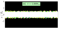
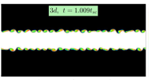
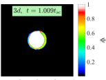
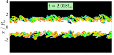
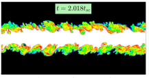
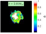
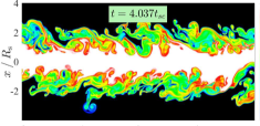
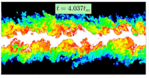
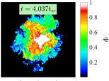
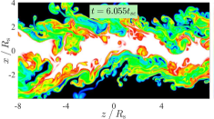
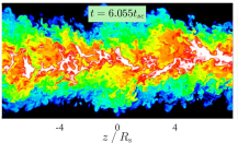
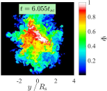
Figure 21: Same as Fig. 2 but for a simulation with $(M_{\rm b},\delta)=(1,10)$. We show snapshots at $t=1,\,2,\,4,$ and $6t_{\rm sc}$. As for the case with $\delta=1$, at $t\sim t_{\rm sc}$ the edge-on distribution of $\psi$ in the 3d cylinder appears nearly identical to its distribution in the 2d slab simulation, while the face-on distribution is dominated by symmetric, $m=0$, and antisymmetric, $m=1$, modes. At $t=2t_{\rm sc}$, the face-on view of the cylinder is dominated by higher-order azimuthal modes, though the edge-on view remains qualitatively similar to the slab despite the appearance of small scale modes. At later times, the 2d slab is still dominated by large scale eddies, while in 3d cylinders the largest eddies have broken up and generated small-scale turbulence, leaving very little unmixed fluid in the stream. By $6t_{\rm sc}$ there is very little unmixed fluid in the 3d stream, while the 2d slab still has a large unmixed core. The break up of the largest eddies and the appearance of small scale modes occurs after a smaller number of stream sound crossing times compared to the case with $\delta=1$ shown in Fig. 2. This is because, as discussed in §4.1, this occurs when $h_{\rm b}\sim 2R_{\rm s}$ which happens after a smaller number of stream sound crossing times for denser streams with longer sound crossing times.

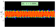
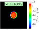
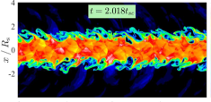
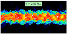
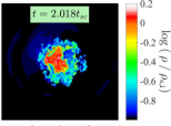
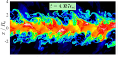
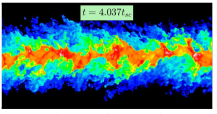
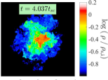
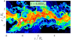
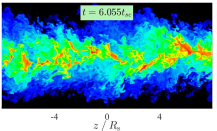
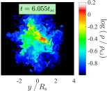
Figure 22: Same as Fig. 21 but where the colour shows the density relative to the initial stream density, $\rho/\rho_{\rm s}$, rather than the passive scalar $\Psi$. At $t\sim t_{\rm sc}$ the density perturbations concentrated near the stream-background interface, characteristic of surface modes. At later times, there are density perturbations in the stream interior as well, driven in part by weak shocks. In the 3d cylinder at late times, the dense regions in the stream interior correspond to the unmixed regions seen in Fig. 21.

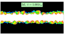
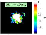
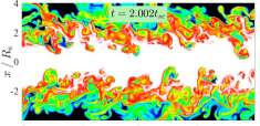
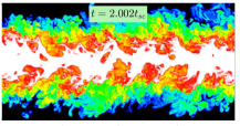
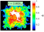
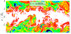
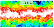
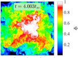
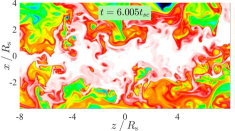
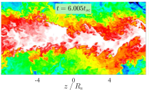
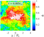
Figure 23: Same as Fig. 21 but for a simulation with $(M_{\rm b},\delta)=(1,100)$. As for the cases with $\delta=1$ and $10$, the edge-on distribution of $\psi$ in the 3d cylinder at $t\sim t_{\rm sc}$ is reasonably similar to its distribution in the 2d slab simulation, though small scale modes are already visible in the 3d simulation since these appear once $h_{\rm b}\sim 2R_{\rm s}$ which happens at $t\sim 0.9t_{\rm sc}$. At later times, the stream expansion rate in the 3d simulation is noticeably slower than in the 2d slab. This is a manifestation of the phenomenon shown in the left panel of Fig. 5 for one case, and mentioned several times in the text of §4, whereby the expansion rate of the shear layer into the background in 3d cylinders decreases to roughly half the value of 2d slabs once $h_{\rm b}\sim 2R_{\rm s}$. Note that at $t\sim 6t_{\rm sc}$ the 3d simulation still contains a lot of unmixed fluid in the stream, since $t_{\rm dis,\,surface}\sim 10t_{\rm sc}$ for this case, according to eq. (9).

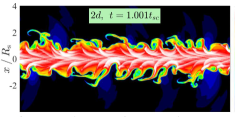
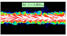
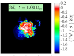
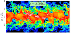
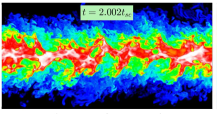
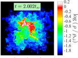
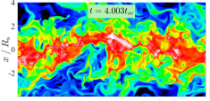
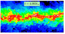
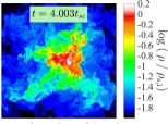
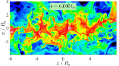
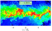
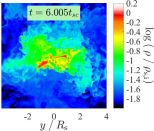
Figure 24: Same as Fig. 23 but where the colour shows the density relative to the initial stream density, $\rho/\rho_{\rm s}$, rather than the passive scalar $\Psi$. Large density fluctuations are visible at $t\sim t_{\rm sc}$, triggered by shocks. These are stronger in 3d than in 2d. $M_{\rm tot}\sim 0.91$ for this simulation, so while body modes are formally stable we are very close to the regime where they are unstable, and they may be triggered by numerical effects, as was also noted by M16, even if the instability is dominated by surface modes. By $t\sim 2t_{\rm sc}$ these density fluctuaions have dissipated as the stream has begun to mix with the background. By $6t_{\rm sc}$ the mean density in the stream has been diluted by a factor of $\sim 10$, with the densest remaining regions corresponding to the few unmixed regions with $\Psi\sim 1$. As also noted in Fig. 23, the 3d cylinder seems to have expanded less than the 2d slab.

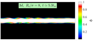
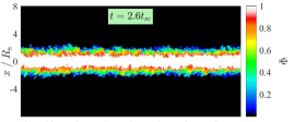
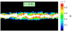
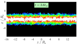
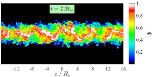
Figure 25: Same as Fig. 12 but for a simulation with $(M_{\rm b},\delta)=(2,10)$. Similar to Fig. 12, the top row shows a snapshot just as $h_{\rm b}$ begins to grow (Fig. 11), while the middle and bottom rows show snapshots 1 and 2 sound crossing times later, respectively. When $\sigma=R_{\rm s}/32$, the stream-background interface is dominated by small-scale structure when $h_{\rm b}$ begins growing, at $t\sim 1.5t_{\rm sc}$. The ensuing growth of $h_{\rm b}$ is due to an expanding shear layer, as in the surface mode simulations described in §4.1. At $\sim 3.6t_{\rm sc}$ there is still an unmixed core at the centre of the stream, which does not fully mix until $t\sim 6t_{\rm sc}$. On the other hand, when $\sigma=R_{\rm s}/8$, the stream-background interface is dominated by a large-scale sinusoidal perturbation with relatively little small scale structure when $h_{\rm b}$ begins growing, at $t\sim 5.3t_{\rm sc}$. By $t\sim 6.3t_{\rm sc}$ a sinusoidal structure with $\lambda\sim 6.5R_{\rm s}$ clearly dominates, in reasonable agreement with the predicted critical wavelength of $\sim 8.5R_{\rm s}$ (Table 1). However, at the same time small scale structure has begun to develop, due to unstable surface modes with high-$m$. Within one additional sound crossing time these small-scale perturbations have efficiently mixed the stream and the background fluids, though the large scale sinusoidal mode is still visible. By $t\sim 7.5t_{\rm sc}$ there is no unmixed fluid left in the stream.

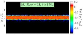
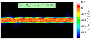
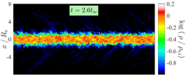
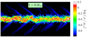
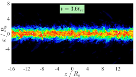
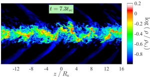
Figure 26: Same as Fig. 25 but where the colour shows the density relative to the initial stream density, $\rho/\rho_{\rm s}$, rather than the passive scalar $\Psi$. The criss-cross patern of density perturbations in the stream interior at early times (top row) is typical of body modes. These are more pronounced in the simulation with $\sigma=R_{\rm s}/8$ because body modes have longer to develop in this case. Once the large scale perturbation has developed and the stream and background begin to mix, the density quickly becomes diluted. Note also the oblique shock waves propagating into the background, which facilitate the transfer of momentum to the background gas in the body mode regime.

References

- Arrigoni Battaia et al. (2018) Arrigoni Battaia F., Prochaska J. X., Hennawi J. F., Obreja A., Buck T., Cantalupo S., Dutton A. A., Macciò A. V., 2018, MNRAS, 473, 3907
- Bassett & Woodward (1995) Bassett G. M., Woodward P. R., 1995, ApJ, 441, 582
- Binney, Nipoti & Fraternali (2009) Binney J., Nipoti C., Fraternali F., 2009, MNRAS, 397, 1804
- Birkinshaw (1990) Birkinshaw M., 1990, The Stability of Jets
- Birnboim & Dekel (2003) Birnboim Y., Dekel A., 2003, MNRAS, 345, 349
- Bodo et al. (1993) Bodo G., Massaglia S., Rossi P., Trussoni E., Ferrari A., 1993, Physics of Fluids, 5, 405
- Bodo et al. (1998) Bodo G., Rossi P., Massaglia S., Ferrari A., Malagoli A., Rosner R., 1998, A&A, 333, 1117
- Bogey, Marsden & Bailly (2011) Bogey C., Marsden O., Bailly C., 2011, Physics of Fluids, 23, 035104
- Bond, Kofman & Pogosyan (1996) Bond J. R., Kofman L., Pogosyan D., 1996, Nature, 380, 603
- Borisova et al. (2016) Borisova E. et al., 2016, ApJ, 831, 39
- Bouché et al. (2016) Bouché N. et al., 2016, ApJ, 820, 121
- Bouché et al. (2013) Bouché N., Murphy M. T., Kacprzak G. G., Péroux C., Contini T., Martin C. L., Dessauges-Zavadsky M., 2013, Science, 341, 50
- Cantalupo et al. (2014) Cantalupo S., Arrigoni-Battaia F., Prochaska J. X., Hennawi J. F., Madau P., 2014, Nature, 506, 63
- Ceverino, Dekel & Bournaud (2010) Ceverino D., Dekel A., Bournaud F., 2010, MNRAS, 404, 2151
- Coles (1985) Coles D., ed., 1985, The uses of coherent structure (Dryden Lecture)
- Danovich et al. (2015) Danovich M., Dekel A., Hahn O., Ceverino D., Primack J., 2015, MNRAS, 449, 2087
- Danovich et al. (2012) Danovich M., Dekel A., Hahn O., Teyssier R., 2012, MNRAS, 422, 1732
- Dekel & Birnboim (2006) Dekel A., Birnboim Y., 2006, MNRAS, 368, 2
- Dekel et al. (2009) Dekel A. et al., 2009, Nature, 457, 451
- Dekel & Mandelker (2014) Dekel A., Mandelker N., 2014, MNRAS, 444, 2071
- Dekel et al. (2013) Dekel A., Zolotov A., Tweed D., Cacciato M., Ceverino D., Primack J. R., 2013, MNRAS, 435, 999
- Dijkstra & Loeb (2009) Dijkstra M., Loeb A., 2009, MNRAS, 400, 1109
- Dimotakis (1986) Dimotakis P. E., 1986, AIAA Journal, 24, 1791
- Dimotakis (1991) Dimotakis P. E., 1991, Turbulent free shear layer mixing and combustion. Tech. rep.
- Efstathiou (1992) Efstathiou G., 1992, MNRAS, 256, 43P
- Elmegreen et al. (2007) Elmegreen D. M., Elmegreen B. G., Ravindranath S., Coe D. A., 2007, ApJ, 658, 763
- Faucher-Giguère et al. (2010) Faucher-Giguère C.-A., Kereš D., Dijkstra M., Hernquist L., Zaldarriaga M., 2010, ApJ, 725, 633
- Faucher-Giguère, Kereš & Ma (2011) Faucher-Giguère C.-A., Kereš D., Ma C.-P., 2011, MNRAS, 417, 2982
- Ferrari, Trussoni & Zaninetti (1981) Ferrari A., Trussoni E., Zaninetti L., 1981, MNRAS, 196, 1051
- Fielding et al. (2017) Fielding D., Quataert E., McCourt M., Thompson T. A., 2017, MNRAS, 466, 3810
- Förster Schreiber et al. (2006) Förster Schreiber N. M., Genzel R., Lehnert M. D., Bouché N., Verma A., Erb D. K., Shapley A. E., et al.,, 2006, ApJ, 645, 1062
- Freund, Lele & Moin (2000) Freund J. B., Lele S. K., Moin P., 2000, Journal of Fluid Mechanics, 421, 229
- Fumagalli et al. (2017) Fumagalli M. et al., 2017, MNRAS, 471, 3686
- Fumagalli et al. (2011) Fumagalli M., Prochaska J. X., Kasen D., Dekel A., Ceverino D., Primack J. R., 2011, MNRAS, 418, 1796
- Genzel et al. (2008) Genzel R., Burkert A., Bouché N., Cresci G., Förster Schreiber N. M., Shapley A., Shapiro K., et al.,, 2008, ApJ, 687, 59
- Genzel et al. (2006) Genzel R., Tacconi L. J., Eisenhauer F., Förster Schreiber N. M., Cimatti A., Daddi E., Bouché N., et al.,, 2006, Nature, 442, 786
- Goerdt & Ceverino (2015) Goerdt T., Ceverino D., 2015, MNRAS, 450, 3359
- Goerdt et al. (2010) Goerdt T., Dekel A., Sternberg A., Ceverino D., Teyssier R., Primack J. R., 2010, MNRAS, 407, 613
- Goerdt et al. (2012) Goerdt T., Dekel A., Sternberg A., Gnat O., Ceverino D., 2012, MNRAS, 424, 2292
- Hardee, Clarke & Howell (1995) Hardee P. E., Clarke D. A., Howell D. A., 1995, ApJ, 441, 644
- Hardee & Stone (1997) Hardee P. E., Stone J. M., 1997, ApJ, 483, 121
- Kereš et al. (2005) Kereš D., Katz N., Weinberg D. H., Davé R., 2005, MNRAS, 363, 2
- Leclercq et al. (2017) Leclercq F. et al., 2017, A&A, 608, A8
- Mandelker et al. (2016) Mandelker N., Padnos D., Dekel A., Birnboim Y., Burkert A., Krumholz M. R., Steinberg E., 2016, MNRAS, 463, 3921
- Mandelker et al. (2018) Mandelker N., van Dokkum P. G., Brodie J. P., van den Bosch F. C., Ceverino D., 2018, ApJ, 861, 148
- Martin et al. (2014a) Martin D. C., Chang D., Matuszewski M., Morrissey P., Rahman S., Moore A., Steidel C. C., 2014a, ApJ, 786, 106
- Martin et al. (2014b) Martin D. C., Chang D., Matuszewski M., Morrissey P., Rahman S., Moore A., Steidel C. C., Matsuda Y., 2014b, ApJ, 786, 107
- Massaglia et al. (1992) Massaglia S., Trussoni E., Bodo G., Rossi P., Ferrari A., 1992, A&A, 260, 243
- Matsuda et al. (2006) Matsuda Y., Yamada T., Hayashino T., Yamauchi R., Nakamura Y., 2006, ApJ, 640, L123
- Matsuda et al. (2011) Matsuda Y. et al., 2011, MNRAS, 410, L13
- Micono et al. (2000) Micono M., Bodo G., Massaglia S., Rossi P., Ferrari A., Rosner R., 2000, A&A, 360, 795
- Murray et al. (1993) Murray S. D., White S. D. M., Blondin J. M., Lin D. N. C., 1993, ApJ, 407, 588
- Nelson et al. (2016) Nelson D., Genel S., Pillepich A., Vogelsberger M., Springel V., Hernquist L., 2016, MNRAS, 460, 2881
- Nelson et al. (2013) Nelson D., Vogelsberger M., Genel S., Sijacki D., Kereš D., Springel V., Hernquist L., 2013, MNRAS, 429, 3353
- Ocvirk, Pichon & Teyssier (2008) Ocvirk P., Pichon C., Teyssier R., 2008, MNRAS, 390, 1326
- Padnos et al. (2018) Padnos D., Mandelker N., Birnboim Y., Dekel A., Krumholz M. R., Steinberg E., 2018, ArXiv e-prints
- Prochaska, Lau & Hennawi (2014) Prochaska J. X., Lau M. W., Hennawi J. F., 2014, ApJ, 796, 140
- Rees & Ostriker (1977) Rees M. J., Ostriker J. P., 1977, MNRAS, 179, 541
- Robertson et al. (2010) Robertson B. E., Kravtsov A. V., Gnedin N. Y., Abel T., Rudd D. H., 2010, MNRAS, 401, 2463
- Spitzer (1956) Spitzer L., 1956, Physics of Fully Ionized Gases
- Springel (2010) Springel V., 2010, MNRAS, 401, 791
- Springel et al. (2005) Springel V. et al., 2005, Nature, 435, 629
- Stark et al. (2008) Stark D. P., Swinbank A. M., Ellis R. S., Dye S., Smail I. R., Richard J., 2008, Nature, 455, 775
- Steidel et al. (2000) Steidel C. C., Adelberger K. L., Shapley A. E., Pettini M., Dickinson M., Giavalisco M., 2000, ApJ, 532, 170
- Stone, Xu & Hardee (1997) Stone J. M., Xu J., Hardee P., 1997, ApJ, 483, 136
- Sutherland & Dopita (1993) Sutherland R. S., Dopita M. A., 1993, ApJS, 88, 253
- Teyssier (2002) Teyssier R., 2002, A&A, 385, 337
- Toro, Spruce & Speares (1994) Toro E. F., Spruce M., Speares W., 1994, Shock Waves, 4, 25
- van de Voort & Schaye (2012) van de Voort F., Schaye J., 2012, MNRAS, 423, 2991
- van de Voort et al. (2012) van de Voort F., Schaye J., Altay G., Theuns T., 2012, MNRAS, 421, 2809
- van de Voort et al. (2011) van de Voort F., Schaye J., Booth C. M., Haas M. R., Dalla Vecchia C., 2011, MNRAS, 414, 2458
- van Leer (1977) van Leer B., 1977, Journal of Computational Physics, 23, 263
- Vietri, Ferrara & Miniati (1997) Vietri M., Ferrara A., Miniati F., 1997, ApJ, 483, 262
- Vogelsberger et al. (2012) Vogelsberger M., Sijacki D., Kereš D., Springel V., Hernquist L., 2012, MNRAS, 425, 3024
- White & Rees (1978) White S. D. M., Rees M. J., 1978, MNRAS, 183, 341
- Xu, Hardee & Stone (2000) Xu J., Hardee P. E., Stone J. M., 2000, ApJ, 543, 161