Electron states in the field of charged impurities in two-dimensional Dirac systems

Abstract

We review the theoretical and experimental results connected with the electron states in two-dimensional Dirac systems paying a special attention to the atomic collapse in graphene. Two-electron bound states of a Coulomb impurity are considered too. A rather subtle role of a magnetic field in the supercritical charge problem in graphene is discussed. The electron states in the field of two equally charged impurities are studied and the conditions for supercritical instability to occur are determined. It is shown that the supercriticality of novel type is realized in gapped graphene with two unlikely charged impurities. For sufficiently large charges of impurities, it is found that the wave function of the occupied electron bound state of the highest energy changes its localization from the negatively charged impurity to the positively charged one as the distance between the impurities increases. The specifics of the atomic collapse in bilayer graphene is considered and it is shown that the atomic collapse in this material is not related to the phenomenon of the fall-to-center.

I Introduction

The phenomenon of the fall-to-center is deeply rooted in the history of physics. The Rutherford’s discovery of the planetary model of the atom immediately brought to the light the problem of the stability of the atom. Indeed, classically, the electron rotating around the nucleus should emit electromagnetic radiation, lose its energy, and fall to the nucleus. We know that the atoms are stable and the atomic collapse is avoided due to the uncertainty principle of quantum mechanics. While the Coulomb interaction scales like $-Ze/r$, where $r$ is the distance to the nucleus and $Ze$ is its charge, the positive electron kinetic energy diverges more strongly $\mathbf{p}^{2}/(2m_{e})\sim\hbar^{2}/(2m_{e}r^{2})$ as $r\to 0$. Therefore, the fall to the nucleus is energetically forbidden.

This qualitative argument shows that the fall-to-center may still be possible in quantum mechanics for more singular potentials $V(r)\sim 1/r^{n}$ with $n\geq 2$. In fact, the Schrödinger equation with the potential $V(r)=-\beta/r^{2}$ provides the canonical textbook example of the fall-to-center in quantum mechanics Landau:t3 , which takes place for $\beta>\hbar^{2}/(8m_{e})$ when the energy spectrum is not bounded from below. If the interaction potential is regularized at some distance $r_{0}$, then the electron wave function of the ground state is localized in the region of the radius $r_{0}$ which shrinks to the origin as $r_{0}\to 0$.

Still physically as $|\mathbf{p}|$ attains the value of order $m_{e}c$, where $c$ is the speed of light, the relativistic effects become relevant. Since the kinetic term in the Dirac equation depends linearly on momentum, the kinetic energy of the electron in the relativistic regime scales like $\hbar/r$ as $r\to 0$. This means that already the Coulomb interaction could lead to the atomic collapse. In quantum electrodynamics (QED) for the regularized Coulomb potential, the atomic collapse takes place for $Z\gtrsim 170$ [Pomeranchuk1945, ; Zeldovich1972, ; Greiner1985, ] when the lowest energy electron bound state dives into the lower continuum transforming into a narrow resonance. This leads to the spontaneous creation of electron-positron pairs with the electrons screening the positively charged nucleus and the positrons emitted to infinity. Since supercritically charged nuclei are not encountered in nature, this phenomenon was never observed in QED. It was suggested in the 70-ties Gershtein1970 ; Rafelski1971 ; Muller1972 ; Zeldovich1972 that the supercritical instability in QED can nevertheless be experimentally tested in a collision of two heavy nuclei. Although subsequent experiments confirmed the existence of supercritical fields in collisions of very heavy nuclei and the gross features of positron emission Greiner1985 , the analysis of the supercritical regime turned out to be a difficult problem mainly due to the transient nature of supercritical fields generated during collisions.

It is an interesting question whether the supercritical instability could be observed in the condensed matter systems. The first natural place to look is the narrow gap semiconductors whose conductance and valence bands are separated by a small gap. There exist also condensed matter systems with the relativistic-like energy spectrum of quasiparticles. Bismuth, whose quasiparticles are described by the massive Dirac equation, provides the historically first example of such a system (for a review, see Refs.Falkovsky1968 ; Edelman1976 ). Long time ago Herring argued Herring1937 that the conductance and valence bands in solids could, in general, meet at discrete touching points. Remarkably, the energy dispersion in the vicinity of these bands touching points is linear and resembles the Weyl equation. The recently discovered Dirac and Weyl semimetals whose itinerant electrons are described by the 3D Dirac and Weyl equations, respectively, experimentally realize the Herring’s prediction (for a review, see, e.g., Ref.Armitage2017 ). However, the corresponding materials are characterized by the large dielectric constants. The small value of the effective coupling constant makes it practically impossible to realize the supercritical instability in these materials.

The situation is different in graphene whose effective coupling constant $\alpha_{g}=e^{2}/(v_{\rm F}\hbar)\approx 2.2$, where $v_{\rm F}\approx c/300$ is the Fermi velocity, exceeds unity. This drastically decreases the value of the critical charge in graphene [Shytov2007a, ; Shytov2007b, ; Pereira2007, ; Fogler2007, ]. Although, according to the theory, the supercritical instability should be easily realized for charged impurities in graphene, its experimental observation remained elusive until recently. The problem is that it is difficult to produce highly charged impurities because of their fast recombination. Still one can reach the supercritical regime by collecting a large enough number of charged impurities in a certain region of graphene. Such an approach was recently successfully realized [Wang2013, ] by using the tip of a scanning tunneling microscope in order to create clusters of charged calcium dimers.

In addition, the external charge in the realistic experimental set-up should be smeared over a finite region of the graphene plane because, otherwise, the Dirac equation is no longer applicable and other nearest $\sigma$-bands should be included in the analysis Fogler2007 . Thus, the potential of charged impurities should be necessarily regularized at small distances in order that the continuum problem be well posed physically. For instance, the charged impurities displaced from the graphene plane provide such a natural regularization and help to avoid the reconstruction of the band spectrum which takes place if they are placed directly into the graphene plane or a disorder is present Feher2009 ; Loktev2012 ; Skrypnik2007 ; Dora2008 .

An interesting aspect of the electron physics in graphene is its two-dimensional character. Therefore, the supercritical instability in the field of a charged impurity in graphene is, in fact, the atomic collapse in a Flatland. Of course, this does not mean that the theory governing the electron-electron interactions in graphene is QED in (2+1) dimensions. Although the electrons are confined in the plane of graphene, the electromagnetic force lines spread beyond the graphene’s plane resulting in the standard Coulomb interaction potential $V_{C}(r)=e^{2}/r$. The crucial advantage of graphene compared to QED is its experimental accessibility where atomic collapse can be investigated in table-top experiments varying such parameters as doping and gate voltage.

The supercritical charge instability is closely related to the excitonic instability in graphene in the strong coupling regime $\alpha>\alpha_{c}\sim 1$ (see, Refs.[Gamayun2009, ; Wang2010, ; Sabio2010, ]) and possible gap opening, which may transform graphene into an insulator Khveshchenko2001 ; Gorbar2002 ; Gorbar2003 ; Khveshchenko2004 ; Gamayun2010 ; Gonzalez2012 ; Drut2009a ; Drut2009b ; Armour2010 ; Buividovich2012 . Indeed, the excitonic instability can be viewed as a many-body analog of the supercritical instability in the field of a charged impurity and the critical coupling $\alpha_{c}$ is an analog of the critical coupling constant $Z_{c}\alpha$ in the problem of the Coulomb center. In the strong coupling regime $\alpha>\alpha_{c}$ the electron can spontaneously create from the vacuum the electron-hole pair (in the same way as the supercritical charge creates electron-hole pairs). The initial electron attracts the hole and forms a bound state (an exciton) and the emitted electron (which also has the supercritical charge) can spontaneously create another pair, etc. The process of creating pairs continues leading to the formation of excitonic condensate and, as a result, the quasiparticles acquire a gap. The semimetal-insulator transition in graphene is similar to the chiral symmetry breaking phase transition in strongly coupled QED studied in the 1970s and 1980s (for a review see Ref.FominReview1983 ). The latter QED transition induced by strong electromagnetic fields was searched in experiments in heavy-ion collisions Peccei1988 .

To stay closer to the experimental situation, one should make a further step by considering electron states in the field of two Coulomb centers, both like and unlike charged. The electron states in the field of charged impurities in graphene and in the presence of a magnetic field are also of considerable interest from the experimental point of view. It was shown in Refs.Luican-Mayer2014 ; Mao2016 that the strength of a charged impurity can be tuned by controlling the occupation of Landau-level states with a gate voltage.

All these topics are considered in the present review paper which is organized as follows. The phenomenon of the supercritical charge instability is briefly discussed in Sec. I. In Sec. II, we analyse the electron states in gapless and gapped monolayer graphene. The experimental data of the observation of the atomic collapse in graphene are provided in Sec. II.3. The impact of a magnetic field on the supercritical charge problem in graphene is studied in Sec. III. Two-electron bound states of a Coulomb impurity are considered in Sec. IV. The atomic collapse in the field of two charged impurities is investigated in Sec. V. The dipole problem is studied in Sec. VI. The specifics of the atomic collapse in bilayer graphene is considered in Sec. VII. The results are summarized and conclusions are given in Sec. VIII.

II Atomic collapse in monolayer graphene

The electron quasiparticle states in the vicinity of the $K_{\pm}$ points of graphene in the potential $V(\mathbf{r})$ of charged impurities are described by the following Dirac Hamiltonian in $2+1$ dimensions:

$$H(\mathbf{p},\xi)=v_{\rm F}\bm{\sigma}\bm{p}+\xi\Delta\sigma_{z}+V(\mathbf{r}),$$ (1)

where $v_{\rm F}$ is the Fermi velocity of graphene, $\bm{p}=-i\bm{\nabla}$ is the canonical momentum, $\sigma_{i}$ are the Pauli matrices, $\Delta$ is a quasiparticle gap, and $\xi$ is an index, which corresponds to the valley $K_{+}$ ($\xi=+1$) or $K_{-}$ ($\xi=-1$). Although the pristine graphene is gapless, a quasiparticle gap $\Delta$ can be generated if graphene sheet is placed on a substrate and two carbon sublattices become inequivalent because of interaction with the substrate (for band structure calculation of such a configuration see, for instance, Ref.Giovannetti2007 ). The gap can arise also in graphene ribbons due to geometrical quantizationSon2006 or due to many-body electron correlations Khveshchenko2001 ; Gorbar2002 ; Gorbar2003 ; Khveshchenko2004 ; Gamayun2010 ; Gonzalez2012 ; Drut2009a ; Drut2009b ; Armour2010 ; Buividovich2012 .

The Hamiltonian (1) acts on two component spinor $\Psi_{\xi s}$ which carries the valley ($\xi=\pm)$ and spin ($s=\pm$) indices. We will use the standard convention: $\Psi^{T}_{+s}=(\psi_{A},\psi_{B})_{K_{+}s}$, whereas $\Psi^{T}_{-s}=(\psi_{B},\psi_{A})_{K_{-}s}$, and $A,B$ refer to two sublattices of hexagonal graphene lattice. Since the interaction potential does not depend on spin, we will omit the spin index $s$ in what follows. Further, for the sake of definiteness, we will consider electrons in the $K_{+}$ valley. The Hamiltonians at two valleys are related by means of the time reversal operator $\Theta=is_{2}\sigma_{1}K$:

$$\Theta H(\mathbf{p},\xi=+1)\Theta^{-1}=H(-\mathbf{p},\xi=-1),$$ (2)

where $s_{2}$ is the Pauli spin matrix and K is the complex conjugation.

The supercritical instability in the field of a single charged impurity was studied quite in detail in the literature Shytov2007a ; Shytov2007b ; Pereira2007 ; Fogler2007 ; Gamayun2009 ; Novikov2007 ; Pereira2008 ; Terekhov2008 ; Shytov2009 ; CastroNeto2009a . In this section we will summarize its main features.

II.1 Resonance states in gapless graphene in quasiclassical approach

Let us start our analysis with the case of gapless graphene. Since massless particles cannot form bound states, the atomic collapse is revealed for massless particles through resonance states which appear when the Coulomb potential strength exceeds a certain critical value $\alpha_{c}=1/2$. In order to demonstrate the presence of these states, it is instructive to begin with the semiclassical analysis. We follow in this subsection the derivation in Ref.Shytov2007a .

In relativistic classical theory, the electron trajectories can spiral around the charged center and eventually fall down on it Darwin1913 if the electron angular momentum is small enough $M<M_{c}=Ze^{2}/c$.

These states can be constructed quasiclassically from relativistic dynamics described by the Hamiltonian $H=v_{\rm F}|\mathbf{p}|+V(r)$, where $V(r)=-Ze^{2}/(\kappa r)$ and $\kappa$ is a dielectric constant. The collapsing trajectories with angular momenta $M<M_{c}=Ze^{2}/(\kappa v_{\rm F})$ are separated from non-falling trajectories by a centrifugal barrier. This is manifested in the expression for the radial momentum square

$$p_{r}^{2}=v_{\rm F}^{-2}\left(E+\frac{Ze^{2}}{\kappa r}\right)^{2}-\frac{M^{2}}{r^{2}}.$$ (3)

Clearly, there is a classically forbidden region, the annulus $r_{1}<r<r_{2}$, $r_{1,2}=(\frac{Ze^{2}}{\kappa}\mp Mv_{\rm F})/|E|$, where the right-hand side of Eq.(3) is negative. The quasi-stationary states trapped by this barrier are obtained from the Bohr-Sommerfeld quantization $\int_{r_{0}}^{r_{1}}p_{r}dr=\pi\hbar n$, where $r_{0}$ is a regularization parameter, which is of order of lattice spacing. Evaluating the integral with logarithmic accuracy, we obtain $\gamma\ln\frac{Ze^{2}}{\kappa r_{0}|E|}=\pi\hbar n$, where $\gamma\equiv\left(M_{c}^{2}-M^{2}\right)^{1/2}$, which gives the quasi-Rydberg states

$$E_{n}\approx-\frac{Ze^{2}}{\kappa r_{0}}e^{-\pi\hbar n/\gamma},\quad n>0.$$ (4)

The energies of these states converge to zero, $E_{n}\to 0$, at large $n$, whereas their radii diverge, similar to the Rydberg states in the hydrogen atoms. To find the transparency of the barrier, we integrate ${\Im m\,}p_{r}$ and obtain the tunneling action

$$S=\int_{r_{1}}^{r_{2}}dr\sqrt{\frac{M^{2}}{r^{2}}-\left(\frac{E}{v_{\rm F}}+\frac{M_{c}}{r}\right)^{2}}=\pi\left(M_{c}-\gamma\right).$$ (5)

Taken near the threshold $\gamma\approx 0$, the transparency $e^{-2S/\hbar}$ gives the width $\Gamma_{n}\sim|E_{n}|\exp(-2\pi Z\alpha)$, where $\alpha=e^{2}/(\kappa\hbar v_{\rm F})$ is the effective coupling constant. The quasi-Rydberg states manifest themselves in the local density of states that can be probed experimentally. Also, resonance scattering on the quasi-bound states manifests itself in the dependence of transport properties on the carrier density. For supercritical potential strength $|Z\alpha|>1/2$ there are oscillations of the Ohmic conductivity which have a characteristic form of Fano resonances centered at $E_{n}$ Shytov2007a . In this regime the conductivity exhibits peaks at the densities for which the Fermi energy $E_{F}$ equals $E_{n}$. The peak position is highly sensitive to the potential strength $Z\alpha$, changing by an order of magnitude when $Z\alpha$ varies from $-1.0$ to $-1.3$.

It is instructive to compare these results to the exact solution of the Coulomb center problem that we do in the next section.

II.2 Supercritical instability in graphene

II.2.1 Gapped graphene, subcritical regime

Now, let us include into consideration a quasiparticle gap that on the one side makes more transparent the derivation of the instability condition (diving of the lowest energy level into the negative continuum), while on the other hand takes into account a possible presence of a gap due to the interaction with a substrate. In this subsection, we follow the study performed in Ref.Gamayun2009 . The electron quasiparticle states in graphene in the field of a single Coulomb impurity are described by Dirac Hamiltonian (1) with a regularized Coulomb potential

$$V(r)=-\frac{Ze^{2}}{\kappa r},\,\,(r>r_{0}),\quad V(r)=-\frac{Ze^{2}}{\kappa r_{0}},\,\,(r<r_{0}).$$ (6)

As we discussed in the Introduction, to avoid the fall-to center problem we should regularize the Coulomb potential at small distances. Potential (6) represents the simplest “cutoff” regularization. Since the Hamiltonian (1) with potential (6) commutes with the total angular momentum operator $J_{z}=L_{z}+S_{z}=-i\hbar\frac{\partial}{\partial\phi}+\frac{\hbar}{2}\sigma_{z}$, we seek eigenfunctions in the following form:

$$\Psi=\frac{1}{r}\left(\begin{array}[]{c}e^{i\phi(j-1/2)}\,a(r)\\ i\,e^{i\phi(j+1/2)}\,b(r)\end{array}\right).$$ (7)

Then we obtain a system of two coupled ordinary differential equations of the first order

$$a^{\prime}-(j+1/2)\frac{a}{r}+\frac{E+\Delta-V(r)}{\hbar v_{\rm F}}b=0,\quad\quad\quad\quad\quad b^{\prime}+(j-1/2)\frac{b}{r}-\frac{E-\Delta-V(r)}{\hbar v_{\rm F}}a=0.\quad\quad\quad\quad$$ (8)

It is convenient to define the quantities $\epsilon={E}/{\hbar v_{\rm F}},\,m={\Delta}/{\hbar v_{\rm F}}$, and $\alpha=\alpha_{g}/\kappa={e^{2}}/{\hbar v_{\rm F}\kappa}$.

The discrete spectrum of Eqs. (8) exists for $|\epsilon|<m$. In this case it is convenient to define

$$u=\sqrt{m^{2}-\epsilon^{2}},\quad\rho=2ur,\quad a=\frac{\sqrt{m+\epsilon}}{2}(g-f),\quad b=\frac{\sqrt{m-\epsilon}}{2}(g+f)$$ (9)

and rewrite Eqs. (8) in the region $r>r_{0}$ as follows:

$$\rho g^{\prime}+g\left(\frac{\rho}{2}-\frac{1}{2}-Z\alpha\frac{\epsilon}{u}\right)+f\left(j+Z\alpha\frac{m}{u}\right)=0,$$

$$\rho f^{\prime}-f\left(\frac{\rho}{2}+\frac{1}{2}-Z\alpha\frac{\epsilon}{u}\right)+g\left(j-Z\alpha\frac{m}{u}\right)=0.$$ (10)

Substituting $f$ from the first equation into the second one, we obtain the equation for the $g$ component

$$\frac{d^{2}g}{d\rho^{2}}+\left(-\frac{1}{4}+\frac{\frac{1}{2}+Z\alpha\frac{\epsilon}{u}}{\rho}+\frac{\frac{1}{4}-j^{2}+Z^{2}\alpha^{2}}{\rho^{2}}\right)g=0,$$ (11)

which is the well-known Whittaker equation Gradshtein-book . Its general solution is

$$g=C_{1}W_{\mu,\nu}(\rho)+C_{2}M_{\mu,\nu}(\rho),\quad\mu=\frac{1}{2}+\frac{Z\alpha\epsilon}{u},\quad\nu=\sqrt{j^{2}-Z^{2}\alpha^{2}}.$$ (12)

Taking into account the asymptotic of the Whittaker functions $W_{k,\nu}(z),M_{k,\nu}(z)$ at infinity,

$$W_{\mu,\nu}(\rho)\simeq e^{-ur}(2ur)^{\mu},\quad M_{\mu,\nu}(\rho)\simeq\frac{\Gamma(1+\nu)}{\Gamma(\frac{1}{2}-\mu+\nu)}\,e^{ur}(2ur)^{-\mu},\quad r\to\infty,$$ (13)

we find that the regularity condition at infinity requires $C_{2}=0$. Then the first equation in (10) gives the following solution for the $f$ component in the region II ($r>r_{0}$):

$$f_{II}=C_{1}\left(j-Z\alpha\frac{m}{u}\right)W_{-\frac{1}{2}+Z\alpha\frac{\epsilon}{u},\nu}(\rho).$$ (14)

Solutions in the region I ($r<r_{0}$) are easily obtained

$$b_{I}=A_{1}\,rJ_{|j+1/2|}\left(r\sqrt{\left(\epsilon+\frac{Z\alpha}{r_{0}}\right)^{2}-m^{2}}\right),$$ (15)

$$a_{I}=A_{1}\,\mbox{sgn}(j)\,\sqrt{\frac{\epsilon+Z\alpha/r_{0}+m}{\epsilon+Z\alpha/r_{0}-m}}\,\,rJ_{|j-1/2|}\left(r\sqrt{\left(\epsilon+\frac{Z\alpha}{r_{0}}\right)^{2}-m^{2}}\right),$$ (16)

where $A_{1}$ is a constant and we took into account the infrared boundary condition which selects only regular solution for $b_{I}$ and $a_{I}$. Energy levels are determined through the continuity condition of the wave function at $r=r_{0}$,

$$\left.\frac{b_{I}}{a_{I}}\right|_{r=r_{0}}=\left.\frac{b_{II}}{a_{II}}\right|_{r=r_{0}},$$ (17)

that gives the equation

$$\frac{W_{\frac{1}{2}+\frac{Z\alpha\epsilon}{u},\nu}(\rho)}{\left(j-\frac{Z\alpha m}{u}\right)W_{-\frac{1}{2}+\frac{Z\alpha\epsilon}{u},\nu}(\rho)}\Big{|}_{r=r_{0}}=\frac{k+1}{k-1},\,\,\,\,k=\mbox{sign}(j)\,\frac{m+\epsilon}{u}\sqrt{\frac{\epsilon+Z\alpha/r_{0}-m}{\epsilon+Z\alpha/r_{0}+m}}\frac{J_{|j+1/2|}(\widetilde{\rho})}{J_{|j-1/2|}(\widetilde{\rho})},\,\widetilde{\rho}=\sqrt{(Z\alpha+\epsilon r_{0})^{2}-m^{2}r_{0}^{2}}.$$ (18)

We analyze this equation in the limit $r_{0}\to 0$ where we can use the asymptotical behavior of the Whittaker function at $\rho\rightarrow 0$,

$$W_{\mu,\nu}(\rho)\simeq\frac{\Gamma(2\nu)}{\Gamma(\frac{1}{2}-\mu+\nu)}\rho^{\frac{1}{2}-\nu}+\frac{\Gamma(-2\nu)}{\Gamma(\frac{1}{2}-\mu-\nu)}\rho^{\frac{1}{2}+\nu}.$$ (19)

In the limit $r_{0}\to 0$ Eq.(18) reduces to the following one,

$$\frac{\Gamma(-2\nu)}{\Gamma(2\nu)}\frac{\Gamma\left(1+\nu-Z\alpha\frac{\epsilon}{u}\right)}{\Gamma\left(1-\nu-Z\alpha\frac{\epsilon}{u}\right)}(2ur_{0})^{2\nu}=-\frac{j+\nu-\frac{Z\alpha(m+\epsilon)}{u}+k_{0}\left(j-\nu-\frac{Z\alpha(m-\epsilon)}{u}\right)}{j-\nu-\frac{Z\alpha(m+\epsilon)}{u}+k_{0}\left(j+\nu-\frac{Z\alpha(m-\epsilon)}{u}\right)}+O(r_{0}),$$ (20)

where

$$k_{0}=\mbox{sign}(j)\,\frac{m+\epsilon}{u}\frac{J_{|j+1/2|}(Z\alpha)}{J_{|j-1/2|}(Z\alpha)}\equiv\frac{m+\epsilon}{u}\,\sigma(Z\alpha,j).$$ (21)

Equation (20) can be rewritten in more convenient form

$$\frac{\Gamma(-2\nu)}{\Gamma(2\nu)}\frac{\Gamma\left(1+\nu-Z\alpha\frac{\epsilon}{u}\right)}{\Gamma\left(1-\nu-Z\alpha\frac{\epsilon}{u}\right)}(2ur_{0})^{2\nu}=-\frac{j-\nu-\frac{Z\alpha(m-\epsilon)}{u}}{j+\nu-\frac{Z\alpha(m-\epsilon)}{u}}\frac{j+\nu-Z\alpha\sigma(Z\alpha,j)}{j-\nu-Z\alpha\sigma(Z\alpha,j)}.$$ (22)

In the limit $r_{0}\to 0$ the energy levels are determined by the poles of the gamma function $\Gamma\left(1+\nu-Z\alpha\frac{\epsilon}{u}\right)$ and by a zero of the right hand side of Eq.(22), this leads to the familiar result (analogue of the Balmer’s formula in QED) Khalilov1998 (rederived also in Novikov2007 ),

$$\epsilon_{n,j}=m\left[1+\frac{Z^{2}\alpha^{2}}{(\nu+n)^{2}}\right]^{-1/2},\quad\left\{\begin{array}[]{c}n=0,1,2,3,...,\,j>0,\\ n=1,2,3,...,\,\hskip 8.53581ptj<0.\end{array}\right.$$ (23)

The bound states for $n\geq 1$ are doubly degenerate, $\epsilon_{n,j}=\epsilon_{n,-j}$. The lowest energy level is given by

$$\epsilon_{0,j=1/2}=m\sqrt{1-(2Z\alpha)^{2}}\,.$$ (24)

If $Z\alpha$ exceeds $1/2$, then the ground state energy (24) becomes purely imaginary, i.e., the fall into the center phenomenon occurs Shytov2007a ; Shytov2007b ; Shytov2009 ; CastroNeto2009a . In fact, all energies $\epsilon_{n,1/2}$ become complex for $Z\alpha>1/2$. The unphysical complex energies indicate that the Hamiltonian of the system is not a self-adjoint operator for supercritical values $Z\alpha>1/2$ and should be extended to become a self-adjoint operator. According to Pomeranchuk1945 ; Zeldovich1972 , nonzero $r_{0}$ resolves this problem. For $Z\alpha>j$, $\nu$ is imaginary for certain $j$ and for such $j$ we denote $\nu=i\beta,\beta=\sqrt{Z^{2}\alpha^{2}-j^{2}}$. For finite $r_{0}$ discrete levels also exist for $Z\alpha>1/2$. Their energy decreases with increasing of $Z\alpha$ until they reach the lower continuum. The behavior of lowest energy levels with $j=1/2$ as functions of the coupling $Z\alpha$ is shown in Fig.1 (left panel).

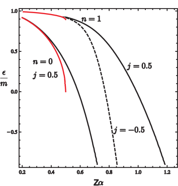
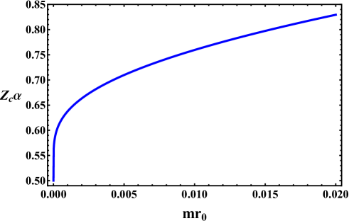
Figure 1: Left panel: The lowest energy levels as functions of $Z\alpha$. Red lines correspond to the pure Coulomb potential (they exist only for $Z\alpha<1/2$); black solid lines are numerical solutions for $j=1/2,\,mr_{0}=0.01$; black dashed line is a numerical solution for $j=-1/2,\,mr_{0}=0.01$. Right panel: The critical coupling as a function of $mr_{0}$ for the $1S_{1/2}$ level.

The critical charge $Z_{c}$ that corresponds to diving into the continuum is obtained from Eq.(22) setting $\epsilon=-m$ there and using the corollary of the Stirling formula: $\frac{\Gamma(x+iy)}{\Gamma(x-iy)}\rightarrow e^{2iy\ln x},\,\,\,\,x\rightarrow+\infty$. We come at the equation

$$e^{-2i\beta\ln(2Z\alpha mr_{0})}=\frac{i\beta-j+Z\alpha\sigma(Z\alpha,j)}{-i\beta-j+Z\alpha\sigma(Z\alpha,j)}\frac{\Gamma(1-2i\beta)}{\Gamma(1+2i\beta)}\,,$$ (25)

or,

$$-\beta\ln(2Z\alpha mr_{0})=\arg\,(Z\alpha\sigma({Z\alpha,j})-j+i\beta)+\arg\,\Gamma(1-2i\beta)+\pi n,\quad n=0,\,1,\,...$$ (26)

It is not difficult to check that for $j=1/2$ and $n=1$ the critical coupling $Z_{c}\alpha$ approaches the value $1/2$ for $mr_{0}\rightarrow 0$. The dependence of the critical coupling $Z_{c}\alpha$ on $mr_{0}$ for $j=1/2$ is shown in the right panel of Fig.1.

II.2.2 Gapped graphene, supercritical regime

Let us analyze Eq. (18) in the supercritical case $Z\alpha>1/2$ and show that there are resonant states for $|\epsilon|>m$ (we define the gap $\Delta>0$). The Whittaker function $W_{\mu,\nu}(\rho)$ with $\mu=1/2+Z\alpha\epsilon/u$, $\nu=\sqrt{j^{2}-Z^{2}\alpha^{2}}$ describes bound states for $|\epsilon|<m$ which are situated on the first physical sheet of the variable $u$ and for which ${\Re e\,}u>0$ (see, Eq.(14)). The quasistationary states are described by the same function $W_{\mu,\nu}(\rho)$ and are on the second unphysical sheet with ${\Re e\,}u<0$. We shall look for the solutions corresponding to the quasistationary states which define outgoing hole waves at $r\to\infty$ with

$${\Re e\,}\epsilon<0,\quad{\Im m\,}\epsilon<0,\quad{\Re e\,}u<0,\quad{\Im m\,}u<0.$$ (27)

For solutions with $Z^{2}\alpha^{2}>j^{2}$ resonance states are determined by Eq.(18) for bound states where $\nu$ is replaced by $\nu=i\beta$. We will consider the states with $j=1/2$ which correspond to the $nS_{\frac{1}{2}}$-states, in particular, the lowest energy state belongs to them. The corresponding equation then takes the form

$$\frac{W_{\frac{1}{2}+\frac{Z\alpha\epsilon}{u},i\beta}(\rho)}{\left(\frac{1}{2}-\frac{Z\alpha m}{u}\right)W_{-\frac{1}{2}+\frac{Z\alpha\epsilon}{u},i\beta}(\rho)}\Big{|}_{r=r_{0}}=\frac{k+1}{k-1},\,\,\,\,k=\,\frac{m+\epsilon}{u}\sqrt{\frac{\epsilon+Z\alpha/r_{0}-m}{\epsilon+Z\alpha/r_{0}+m}}\frac{J_{1}(\widetilde{\rho})}{J_{0}(\widetilde{\rho})},\,\widetilde{\rho}=\sqrt{(Z\alpha+\epsilon r_{0})^{2}-m^{2}r_{0}^{2}}.$$ (28)

The analytical results can be obtained for the near-critical values of $Z$ when $Z\alpha-1/2\ll 1$. We assume that $|2ur_{0}|\ll 1$, then using the asymptotic of the Whittaker function, we find

$$(2ur_{0})^{2i\beta}\frac{\Gamma(1-2i\beta)}{\Gamma(1+2i\beta)}\frac{\Gamma\left(1+i\beta-\frac{Z\alpha\epsilon}{u}\right)}{\Gamma\left(1-i\beta-\frac{Z\alpha\epsilon}{u}\right)}=\frac{\frac{1}{2}-i\beta-\frac{Z\alpha(m-\epsilon)}{u}}{\frac{1}{2}+i\beta-\frac{Z\alpha(m-\epsilon)}{u}}\frac{\frac{1}{2}+i\beta-Z\alpha\frac{J_{1}(Z\alpha)}{J_{0}(Z\alpha)}}{\frac{1}{2}-i\beta-Z\alpha\frac{J_{1}(Z\alpha)}{J_{0}(Z\alpha)}}\,.$$ (29)

Expanding Eq.(29) in the near critical region in powers of $\beta=\sqrt{Z^{2}\alpha^{2}-1/4}$, we find the following equation:

$$(-2i\sqrt{\epsilon^{2}-m^{2}}r_{0})^{2i\beta}=1+4i\beta\left[\frac{J_{0}(1/2)}{J_{0}(1/2)-J_{1}(1/2)}+\Psi(1)-\frac{1}{2}\Psi\left(1-\frac{i}{2}\frac{\epsilon}{\sqrt{\epsilon^{2}-m^{2}}}\right)-\frac{1}{1+i\sqrt{\frac{\epsilon-m}{\epsilon+m}}}\right].$$ (30)

Here $\Psi(x)$ is the psi-function and we put $u=-i\sqrt{\epsilon^{2}-m^{2}}$ where ${\Im m}\sqrt{\epsilon^{2}-m^{2}}<0$ on the second sheet.

It is instructive to consider resonant states in the vicinity of the level $\epsilon=-m$ when bound states dive into the lower continuum and determine their real and imaginary parts of energy. First of all, nonzero $m$ increases the value of the critical charge. Indeed, using Eq.(26), we obtain that the critical value $Z_{c}\alpha$ for $j=1/2$ scales with $m$ like (see Fig.1 (right panel))

$$Z_{c}\alpha\simeq\frac{1}{2}+\frac{\pi^{2}}{\ln^{2}(cmr_{0})},\quad c=\exp\left[-2\Psi(1)-\frac{2J_{0}(1/2)}{J_{0}(1/2)-J_{1}(1/2)}\right]\approx 0.21.$$ (31)

Note that the dependence of the critical coupling on $mr_{0}$ is quite similar to that in the strongly coupled QED Fomin1978 ; FominReview1983 .

For $Z>Z_{c}$, using Eq.(30), we find the following resonant states:

$$\epsilon=-m\left(1+b+i\frac{3\pi}{8}e^{-\pi/\sqrt{2b}}\right),\quad b=\frac{3\pi}{8}\,\frac{\beta-\beta_{c}}{\beta\beta_{c}},$$ (32)

where $\beta_{c}=\sqrt{(Z_{c}\alpha)^{2}-1/4}$. Like in QED Popov1971 the imaginary part of energy of these resonant states vanishes exponentially as $Z\to Z_{c}$. Such a behavior is connected with tunneling through the Coulomb barrier in the problem under consideration. For the quasielectron in graphene in a central potential $V(r)$, expressing the lower component of the Dirac spinor (7) through the upper one and following Zeldovich1972 ; Popov1971 , we obtain an effective second order differential equation in the form of the Schrödinger equation

$$\chi^{\prime\prime}(r)+k^{2}(r)\chi(r)=0,\quad\quad\quad a(r)=\exp\left[\frac{1}{2}\int\left(\frac{1}{r}-\frac{\tilde{V}^{\prime}}{\epsilon+m-\tilde{V}}\right)\,dr\right]\,\chi(r).$$ (33)

Here

$$k^{2}(r)=2(\mathcal{E}-U(r)),\quad\mathcal{E}=\frac{\epsilon^{2}-m^{2}}{2},\quad\tilde{V}=\frac{V}{\hbar v_{\rm F}},$$ (34)

and we represent the effective potential as the sum of two terms $U=U_{1}+U_{2}$, where $U_{1}$ is the effective potential for the Klein–Gordon equation and $U_{2}$ takes into account the spin dependent effects,

$$U_{1} = \epsilon\tilde{V}-\frac{\tilde{V}^{2}}{2}+\frac{j(j-1)}{2r^{2}},$$ (35)

$$U_{2} = \frac{1}{4}\left[\frac{\tilde{V}^{\prime\prime}}{\epsilon+m-\tilde{V}}+\frac{3}{2}\left(\frac{\tilde{V}^{\prime}}{\epsilon+m-\tilde{V}}\right)^{2}+\frac{2j\tilde{V}^{\prime}}{r(\epsilon+m-\tilde{V})}\right].$$ (36)

Note that Eq.(33) and the potentials (35), (36) coincide with the corresponding equations in QED Zeldovich1972 . One can show that in the near-critical regime ($Z\to Z_{c}$, $j=1/2$, and $\epsilon=-m$) the effective potential $U(r)$ has the Coulomb barrier (see Fig.3 below), which prevents the delocalization of the wave function.

The tight-binding approach (solved exactly by using numerical techniques) was compared with the continuum approach based on the Dirac equation in Ref.Pereira2007 . It was shown that the latter provides a good qualitative description of the problem at low energies when properly regularized. On the other hand, the Dirac description fails at moderate to high energies and at short distances when the lattice description should be used.

II.2.3 Gapless graphene

We consider now the case of gapless graphene, $m=0$. Writing $\epsilon=|\epsilon|e^{i\gamma}$ Eq.(30) takes the form

$$\ln(2|\epsilon|r_{0})+i\left(\gamma-\frac{\pi}{2}\right)\simeq 2\left[\frac{J_{0}(1/2)}{J_{0}(1/2)-J_{1}(1/2)}+\Psi(1)-\frac{1}{2}\Psi\left(1-\frac{i}{2}\right)-\frac{1}{1+i}\right]-\frac{\pi n}{\beta},\quad n=1,2,\dots.$$ (37)

We find

$$\epsilon^{(0)}_{n}=ar_{0}^{-1}e^{i\gamma}\exp\left[-\frac{\pi n}{\sqrt{Z^{2}\alpha^{2}-1/4}}\right]=-(1.18+0.17i)r_{0}^{-1}\exp\left[-\frac{\pi n}{\sqrt{Z^{2}\alpha^{2}-1/4}}\right],\quad n=1,2,\dots,$$ (38)

where

$$\gamma=\frac{\pi}{2}\left(1+\coth\frac{\pi}{2}\right)\approx 3.28,\quad a=\frac{1}{2}\exp\left[\frac{2J_{0}(1/2)}{J_{0}(1/2)-J_{1}(1/2)}+2\Psi(1)-1-{\Re e\,}\Psi\left(1-\frac{i}{2}\right)\right]\approx 1.19.$$ (39)

These results are in agreement with Eq. (4) and Refs.Shytov2007a ; Shytov2007b . The energy of quasistationary states (38) has a characteristic essential-singularity type dependence on the coupling constant reflecting the scale invariance of the Coulomb potential. The infinite number of quasistationary levels is related to the long-range character of the Coulomb potential. Note that a similar dependence takes place in the supercritical Coulomb center problem in QED FominMiransky1976 .

Since the “fine structure constant” $e^{2}/\hbar v_{\rm F}\approx 2.2$ in graphene, an instability could potentially appear already for the charge $Z=1$. However, in the analysis above we did not take into account the vacuum polarization effects. Considering these effects and treating the electron-electron interaction in the Hartree approximation, it was shown in Ref.Terekhov2008 that the effective charge of impurity $Z_{\rm eff}$ is such that the impurity with bare charge $Z=1$ remains subcritical, $Z_{\rm eff}e^{2}/(\kappa\hbar v_{\rm F})<1/2$, for any coupling $e^{2}/(\kappa\hbar v_{\rm F})$, while impurities with higher $Z$ may become supercritical.

For finite $m$ and in the case $|\epsilon|\gg m,\,\,\Re e\,\epsilon<0$, expanding Eq.(30) in $m/\epsilon$ we get up to the terms of order $m^{2}/\epsilon^{2}$,

$$\epsilon-\frac{m^{2}}{2\epsilon}=\epsilon^{(0)}_{n}\left(1-\frac{m}{\epsilon}+\frac{m^{2}}{\epsilon^{2}}(0.29-0.23i)\right),\quad\quad\quad n=1,2,\dots\,.$$ (40)

The resonant states with $\epsilon^{(0)}_{n}$ describe the spontaneous emission of positively charged holes when electron bound states dive into the lower continuum in the case $m=0$. In order to find corrections to these energy levels due to nonzero $m$, we seek solution of Eq.(40) as a series $\epsilon=\sum\limits_{k=0}^{\infty}\epsilon^{(k)}$ with $\epsilon^{(k)}$ of order $m^{k}$ and easily find the first two terms

$$\epsilon_{n}=\epsilon_{n}^{(0)}-m+\frac{m^{2}}{|\epsilon^{(0)}_{n}|}(0.24+0.20i).$$ (41)

Since ${\Im m\,}\epsilon_{n}^{(0)}<0$, the appearance of a gap results in decreasing the width $|{\rm Im}\epsilon|$ of quasistationary states and, therefore, increases stability of the system. Also, as we showed above, the critical value $Z_{c}\alpha(mr_{0})$, determined by the condition of appearance of a nonzero imaginary part of the energy, increases with the increase of $m$. Thus there are two possibilities for the system with supercritical charge to become stable: to create spontaneously electron-holes pairs and shield the charge or to generate spontaneously the quasiparticle gap. In the problem of the supercritical Coulomb center only the first possibility can be realized, which is already due to the formulation of the problem as the one-particle one. The second possibility - dynamical generation of the gap - was studied in Refs. Gamayun2009 ; Wang2010 ; Sabio2010 ; Khveshchenko2001 ; Gorbar2002 ; Gorbar2003 ; Khveshchenko2004 ; Gamayun2010 ; Gonzalez2012 ; Drut2009a ; Drut2009b ; Armour2010 ; Buividovich2012 .

Considering the many-body problem of strongly interacting gapless quasiparticles in graphene, it was shown that the Bethe-Salpeter equation for an electron-hole bound state contains a tachyon in its spectrum in the supercritical regime $\alpha>\alpha_{c}$, the critical constant $\alpha_{c}=1.62$ in the static random-phase approximation Gamayun2009 and $\alpha_{c}=0.92$ in the case of the frequency-dependent polarization function Gamayun2010 . The tachyon states play the role of quasistationary states in the problem of the supercritical Coulomb center and lead to the rearrangement of the ground state and the formation of excitonic condensate. Thus, there is a close relation between the two instabilities, in fact, the tachyon instability can be viewed as the field theory analog of the fall-to-center phenomenon and the critical coupling $\alpha_{c}$ is an analog of the critical coupling $Z_{c}\alpha$ in the problem of the Coulomb center. The physics of two instabilities is related to strong Coulomb interaction.

II.3 Experimental observation of the atomic collapse in graphene

Univalent charge impurities, such as K, Na, or ${\rm NH_{3}}$, all commonly used in graphene, are on the border of the supercritical regime. To investigate this regime experimentally, one can use divalent or trivalent dopants such as alkaline-earth or rare-earth metals. However, the observation of atomic collapse in the field of supercritical impurities has remained elusive for some time due to the difficulty of producing highly charged impurities.

For the first time, the supercritical Coulomb behavior was observed in atomically-fabricated “artificial nuclei” assembled on the surface of a gated graphene device in Ref.Wang2013 . Calcium atoms were deposited onto the graphene device at low temperature $T<10\,K$. Then graphene was warmed up before returning to lower temperature, thus causing the Ca adatoms to thermally diffuse and bind into dimers. Further, as charges are transferred from a Ca dimer into graphene band states, the Ca dimer becomes positively charged. By making use of the density functional theory calculations, it was found that Ca dimers acquire an effective positive charge $0.4\,e$.

The tunable charge centers were synthesized by pushing together Ca dimers using the tip of a scanning tunneling microscope (STM) (see insets to Fig. 2, a to c), thus allowing creation of supercritical Coulomb potentials from subcritical charge elements. The scanning tunneling spectroscopy was used to observe the emergence of atomic-collapse electronic states extending further than 10 nm from the center of artificial nuclei in the supercritical regime ($Z>Z_{\rm c}$). Here, the effective charge $Z$ is defined as the screened cluster charge where the effects of intrinsic screening due to graphene band polarization and the substrate are taken into account, and the critical value is $Z_{c}=\hbar v_{F}/2e^{2}\sim 0.25$. By tuning the graphene Fermi level ($E_{\rm F}$) via electrostatic gating the atomic collapse behavior was observed.

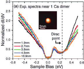
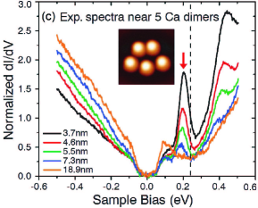
Figure 2: Evolution of charged impurity clusters from subcritical to supercritical regime. (a-c) $dI/dV$ spectra measured at different distances from the center of Ca-dimer clusters (i.e., artificial nuclei) composed of 1, 4, and 5 dimers. “Center” here is defined as the average coordinate of dimers within a cluster. All spectra were acquired at the same back-gate voltage ($V_{g}=-30\,{\rm V}$) and each was normalized by a different constant factor to account for exponential changes in conductivity due to location-dependent tip-height changes Wang2012 ; Li1997 ; Wittneven1998 . Insets: STM topographs of atomically fabricated Ca-dimer clusters. The nuclear charges $Z/Z_{\rm c}$ of (a) 0.5 (1-dimer cluster), (b) 1.8 (4-dimer cluster), and (c) 2.2 (5-dimer cluster). Black dashed lines indicate Dirac point, red arrows indicate atomic collapse state observed in experiment. This figure is an adapted version of the corresponding figure from Ref. Wang2013 .

Experimentally, the local density of states (LDOS) is measured by means of the STM technique. A sharp STM tip scans over a graphene piece and measures the electric current $I$ from the surface due to the tunneling effect. This current depends on the voltage $V$ between tip and a sample and its derivative with respect to $V$ is proportional to the LDOS, $dI/dV\sim D(E,\mathbf{r})$ where $D(E,\mathbf{r})$ is given by Eq.(64) below. The curves in Fig.2 show the differential conductance $dI/dV$ (and thus the LDOS) as a function of the bias voltage $V$, hence the energy $E=eV$. The various curves in panels (a-c) correspond to different distances from the charge center in the range of about $2-20\mbox{nm}$.

Spectra acquired near 1-dimer clusters (Fig. 2a) displayed electron-hole asymmetry as well as an extra oscillation in the LDOS at high energies above the Dirac point. For the 4-dimer cluster, the resonance is clearly observed close to the Dirac point (Fig. 2b). For the 5-dimer cluster, the resonance shifts below the Dirac point (Fig. 2c). The formation of this resonance (or quasi-bound state) as nuclear charge increases is the “smoking gun” for the atomic collapse. The experimental data suggest that clusters with just one or two Ca dimers are in the subcritical regime. The clusters composed of four or more dimers are either (for four dimers) transitioning into or (for five dimers) have fully entered the supercritical regime, as evidenced from panels (b) and (c) in Fig.2. For these clusters, $Z/Z_{\rm c}$ is determined by matching the quasi-bound state resonance energy between the simulation and experiment. The main features seen in the experimental data are well reproduced by the Dirac equation simulations in Ref.Wang2013 .

In order to check that the magnitude of $Z/Z_{\rm c}$ extracted for Ca dimers from the Dirac equation fits is physically reasonable, a completely separate density functional theory calculation of the charge state expected for a Ca dimer adsorbed to graphene was performed [Wang2013, ]. This calculation (which had no fitting parameters) yielded a single-dimer charge ratio of $Z/Z_{\rm c}=0.6\pm 0.3$. This is in agreement with the value $Z/Z_{\rm c}=0.5\pm 0.1$ obtained via Dirac equation simulations, and thus lends further support to overall interpretation of the data. The behavior of the quasi-bound state observed for high-$Z$ artificial nuclei depends on whether it is occupied by electrons or empty. For the details of this doping dependence see the original paper Wang2013 .

III Supercritical instability in a magnetic field

As we discussed in the Introduction, the supercritical charge instability in a many-body system leads to much more dramatic consequences compared to the single-particle problem of the Coulomb center. Like the Cooper instability in the theory of superconductivity, the QED supercritical coupling instability is resolved only through the formation of a condensate of electron-positron pairs generating a mass gap in the spectrum FominReview1983 . It was shown in Krive1992 ; Klimenko1991 ; Gusynin1994 ; Gusynin1996 that magnetic field catalyses gap generation in relativistic-like systems and even the weakest attraction leads to the formation of a symmetry breaking condensate. Therefore, the many-body system is always in the supercritical regime once there is an attractive interaction. The magnetic catalysis plays an important role in quantum Hall effect studies in graphene graphene-QHE , where it is responsible for lifting the degeneracy of the Landau levels.

In QED in (3+1) dimensions, the Coulomb center problem in a magnetic field was studied for massive fermions in Oraevski1977 ; Schlutter1985 . There it was found that the magnetic field confines the transverse electronic motion and the electron in a magnetic field is closer to the nucleus than in the case where magnetic field is absent. Thus, it feels stronger Coulomb field. Therefore, $Z_{c}\alpha$ decreases with $B$. The Dirac equation for (2+1)-dimensional quasiparticles in graphene in the Coulomb potential in a magnetic field was considered in Ref.Khalilov-attempt where exact solutions were found for certain values of magnetic field, i.e., this problem furnishes an example of the so-called quasi-exactly solvable models. However, no instability or resonance was found.

We would like to stress that the presence of a constant magnetic field changes qualitatively the supercritical Coulomb center problem. Indeed, if magnetic field is absent, then the supercritical Coulomb center instability leads to a resonance which describes an outgoing positron propagating freely to infinity. However, since charged particles in a plane perpendicular to a magnetic field do not propagate freely to infinity, such a behavior is impossible for the in-plane Coulomb center problem in graphene in an out-of-plane magnetic field. Therefore, a priori it is not clear how the supercritical instability manifests itself in the Coulomb center problem in a magnetic field. This question was studied in Ref. Gamayun2011 . We would like to note that the role of a magnetic field for the atomic collapse in graphene is rather subtle and different conclusions on this issue were drawn in the literature Siedentop2012 ; Yang2014 ; Moldovan2017 .

In the presence of a charged impurity, degenerate Landau levels convert into bandlike structures due to lifting the orbital degeneracy. For zero chemical potential, as the charge of impurity increases, the energy level with the quantum numbers $n=0$, $j=-1/2$ comes close to the highest energy state of the level $n=-1$. In the absence of magnetic field, the corresponding bound state would dive into the lower continuum and further increase of the charge of impurity would produce a resonance. The situation is qualitatively different in the presence of a magnetic field as the energy curves with the same momenta $j$ never cross. The results clearly demonstrate this phenomenon of the level repulsion between the sublevels with the same $j$ and the formation of a quasiresonance state when the impurity charge exceeds a critical value. In such a case we observe a redistribution of profiles of radial distribution functions with the same orbital momentum among lower Landau levels $n\leq-1$.

III.1 The Coulomb center in a magnetic field

Let us consider the electron states in gapped graphene with a single charged impurity in a magnetic field. The corresponding Hamiltonian could be obtained from Eq.(1) by the standard substitution $\mathbf{p}\to\bm{\pi}=-i\hbar\bm{\nabla}+\frac{e}{c}\mathbf{A}$, where $-e<0$ is the electron charge and the vector potential $\mathbf{A}=B/2(-y,\ x)$ in the symmetric gauge describes magnetic field perpendicular to the plane of graphene. We regularize the Coulomb potential of an impurity by introducing a parameter $r_{0}$ of the order of the graphene lattice spacing. Then the regularized interaction potential of the impurity with charge $Ze$ is given by

$$V\left(\mathbf{r}\right)=-\frac{Ze^{2}}{\kappa\sqrt{r^{2}+r_{0}^{2}}}.$$ (42)

It is convenient to introduce the magnetic length $l_{B}=\sqrt{{\hbar c}/{|eB|}}$ and the dimensionless quantity $\zeta=Ze^{2}/(\kappa\hbar v_{\rm F})$ which characterizes the strength of the bare impurity. Since the total angular momentum is conserved, we use the polar coordinates $(r,\ \phi)$ and seek eigenfunctions in the form (7). Then the Dirac equation takes the form

$$\left\{\begin{array}[]{c}a^{\prime}-\frac{j+1/2}{r}a-\frac{r}{2l_{B}^{2}}a+\frac{E+\xi\Delta-V(r)}{\hbar v_{\rm F}}b=0,\\ b^{\prime}+\frac{j-1/2}{r}b+\frac{r}{2l_{B}^{2}}b-\frac{E-\xi\Delta-V(r)}{\hbar v_{\rm F}}a=0.\end{array}\right.$$ (43)

Eliminating, for example the function $a(r)$, one can get a second order differential equation for $\chi(r)$ defined by the relation

$$[E-\xi\Delta-V(r)]^{1/2}\chi(r)=\frac{b(r)}{\sqrt{r}}.$$ (44)

We obtain the following Schrödinger-like equation:

$$-\chi^{\prime\prime}(r)+U(r)\chi(r)=\mathcal{E}\chi(r),$$ (45)

where

$$\mathcal{E}=\frac{E^{2}-\Delta^{2}}{(\hbar v_{\rm F})^{2}},$$ (46)

and the effective potential, $U=U_{1}+U_{2}$, reads

$$U_{1} = \frac{V(2E-V)}{(\hbar v_{\rm F})^{2}}+\frac{j(j+1)}{r^{2}}+\frac{r^{2}}{4l_{B}^{4}}+\frac{j-1/2}{l_{B}^{2}},$$ (47)

$$U_{2} = \frac{1}{2}\left[\frac{V^{\prime\prime}}{E-\xi\Delta-V}+\frac{3}{2}\left(\frac{V^{\prime}}{E-\xi\Delta-V}\right)^{2}-\left(\frac{j}{r}+\frac{r}{2l_{B}^{2}}\right)\frac{2V^{\prime}}{(E-\xi\Delta-V)}\right].$$ (48)

We plot the effective potential $U(r)$ near the $K_{-}$ point ($\xi=-1$) for $E=-\Delta$ and $j=-1/2$ in Fig. 3, where the energy barrier in the absence of magnetic field is clearly seen, which leads to the appearance of resonances for sufficiently large charge. We note that the equations for spinor components $a(r)$ and $b(r)$ at the $K_{-}$ point can be obtained from the equations in Sec.IIB1 at the $K_{+}$ point by interchanging $a\leftrightarrow b$ and changing $j\rightarrow-j$ since two points are related by means of the time reversal transformation, $\Psi_{K_{-}}=\Theta\Psi_{K_{+}}$, introduced in Sec.II. The presence of a magnetic field changes the asymptotic of the effective potential at infinity and, thus, forbids the occurrence of resonance states. This feature distinguishes qualitatively the Coulomb center problem in a magnetic field from that at $B=0$.

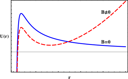
Figure 3: The potential $U(r)$ as a function of a distance from the Coulomb center at zero and nonzero magnetic field, near the $K_{-}$ point for $E=-\Delta$ and $j=-1/2$.

Unfortunately, Eq.(45) belongs to the class of equations with two regular and one irregular singular (at $r=\infty$) points, and cannot be solved in terms of known special functions. In the regime $Z\alpha\to 0$, we can find it using perturbation theory. For $Z\alpha=0$, the corresponding solutions are the well known Landau states degenerate in the total angular momentum $j$. The Coulomb potential of impurity removes degeneracy in $j$ and the eigenenergies split into series of sublevels resulting in an $j$ dependent energy $E_{nj}$. The energy downshift is largest for $E_{0j}$ and diminishes with increasing $-j$. For the $n=0$ level with $E_{0j}^{(0)}=E_{0}^{(0)}=\Delta$ the normalized wave function has the form (at the $K_{-}$ point)

$$\Psi_{M}(r,\phi)=\frac{(-1)^{M}}{l_{B}\sqrt{2\pi M!}}e^{-r^{2}/4l_{B}^{2}}\left(\begin{array}[]{c}0\\ \left(\frac{r^{2}}{2l_{B}^{2}}\right)^{M/2}e^{-iM\phi}\end{array}\right),$$ (49)

where $M=-(j+1/2)=0,\,1,\,2,...$ is the orbital quantum number. Energy corrections $\varepsilon_{M}$ of perturbed states of the Landau level $E_{0}^{(0)}=\Delta$ are found from the secular equation

$$|\varepsilon-V_{M_{1}M_{2}}|=0,$$ (50)

where $V_{M_{1}M_{2}}$ is a matrix element of the potential on states (49). Since $V_{M_{1}M_{2}}$ is a diagonal matrix, we easily obtain

$$\varepsilon_{M}=V_{MM}=-\frac{Ze^{2}}{M!2^{M}\kappa l_{B}}\int\limits_{0}^{\infty}\frac{d\rho\,\rho^{2M+1}\,e^{-\rho^{2}/2}}{\sqrt{\rho^{2}+\rho_{0}^{2}}}=-\frac{Ze^{2}}{2^{M+1}\kappa l_{B}}\rho_{0}^{2M+1}\Psi\left(1+M,3/2+M;\rho_{0}^{2}/2\right)\,,$$ (51)

where $\Psi(a,c;z)$ is the confluent hypergeometric function, $\rho_{0}=r_{0}/l_{B}$. For small $Z\alpha\ll 1$ we can use the unregularized Coulomb potential, then setting $\rho_{0}=0$ in Eq.(51) we get

$$\varepsilon_{M}=-\frac{Ze^{2}\Gamma(M+\frac{1}{2})}{\kappa l_{B}\sqrt{2}\Gamma(M+1)}.$$ (52)

Thus at large $M$ the energy levels accumulate near the value $E=\Delta$,

$$E_{0M}=E^{(0)}_{0}+\varepsilon_{M}\simeq\Delta-\frac{Ze^{2}}{\kappa l_{B}\sqrt{2M}}.$$ (53)

The largest correction by modulus $\varepsilon_{0}=-Z\alpha\hbar v_{\rm F}\sqrt{\pi}/l_{B}\sqrt{2}$ is for the state with $M=0$. Naturally, in the lowest order of perturbation theory, the energy linearly decreases with the increase of the impurity charge. The numerical solution of Eq. (45) shows that this behavior changes when the charge exceeds a certain critical value and after that the level repulsion occurs (see Fig. 4).

For finite $\Delta$ one can define the critical charge by the condition $E=E_{0}^{(0)}+\varepsilon_{0}=-\Delta$ when the lowest energy empty level descending from the upper continuum crosses the energy level of a filled state. In the regime of small coupling, $Z\alpha\ll 1$ and $\Delta l_{B}\ll 1$, this gives

$$Z_{c}\alpha=\frac{2\sqrt{2}\Delta l_{B}}{\sqrt{\pi}\hbar v_{\rm F}}\,.$$ (54)

Clearly, this critical charge tends to zero as $\Delta\to 0$, while the state with $M=0$ of the zero Landau level moves below zero energy for any small impurity charge (its energy is $\varepsilon_{0}=-Z\alpha\hbar v_{\rm F}\sqrt{\pi}/l_{B}\sqrt{2}$). The states connected with the zero Landau level play an important role in the many-body problem, e.g., in the formation of the excitonic condensate and gap generation for quasiparticles Gorbar2002 ; Semenoff1999 due to the magnetic catalysis. In the case of a charged impurity in a magnetic field, the negative energy states are filled and it is physically more sensible to connect the critical charge with the anticrossing of Landau levels in the negative energy region (see the discussion below).

Although, in view of the magnetic catalysis Gusynin1994 , a nonzero gap is always generated in graphene in a perpendicular magnetic field Khveshchenko2001 ; Gorbar2002 ; Gorbar2003 ; Khveshchenko2004 , this gap is rather small for realistic magnetic fields. Therefore, it makes sense to neglect it and see how levels with the same $j$ evolve. Let us solve Eqs. (43) numerically by using the shooting method. In order to utilize this method, one should determine the appropriate asymptote of the solution at $r\to 0$ for $|V(r)|\approx|V(0)|=\frac{Ze^{2}}{\kappa r_{0}}\gg|E|$. At the $K_{+}$ point it is convenient to introduce the orbital quantum number $m=j-1/2=-M-1$. Then, for $m\geq 0$ ($j\geq 1/2$) the upper component of (7) dominates and the leading behavior is $a(r)\sim r^{m+1}$, for $m<0$ ($j<1/2$) the lower component dominates with $b(r)\sim r^{-m}$ (see Ref. [Sobol2016, ]).

The numerical integration of Eq. (43) proceeds as follows. We take a “shot” from $r=0$ at a fixed value of energy solving the differential equations with the correct initial conditions and check the behavior of the wave functions at $r\to\infty$. The latter may tend to $+\infty$ for some values of energy or to $-\infty$ for other values. A physical solution is the solution for which the exponentially growing behavior of the absolute value is absent. We find the corresponding value of the energy of this solution by using the method of bisections. In all numerical calculations, we use $r_{0}=0.05l_{B}$.

The magnetic field modifies the energy spectrum of electrons in the Coulomb field of the charged impurity making all continuum states discrete and provides an effective scale given by the magnetic length. On the other hand, the charged impurity removes the orbital degeneracy of Landau levels transforming the latter into bandlike structures. Figure 4 (left panel) shows the colormap of the LDOS at the impurity position as a function of coupling $\zeta$ and dimensionless energy ${El_{B}}/{\hbar v_{\rm F}}$ in the magnetic field $B=10$ T. Red lines correspond to Landau levels split into sublevels with different orbital numbers. At the beginning, the curves decrease linearly in accordance with Eq. (52). As the charge of impurity increases, the curves, which correspond to the $n=0,\,1$ Landau levels come close to lower curves, which form a “quasicontinuum”. In the absence of magnetic field, with further increase of the charge of impurity the corresponding bound state would dive into the lower continuum producing a resonance.

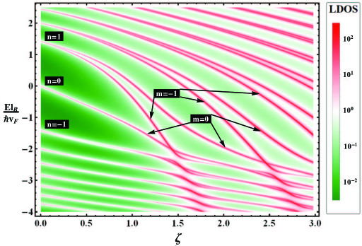
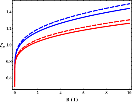
Figure 4: Left panel: The colormap of the LDOS at the impurity position ($r=0$) as a function of coupling $\zeta$ and energy $E$ in the magnetic field $B=10$ T. Black labels indicate the Landau level numbers $n$ and orbital quantum numbers $m$. Right panel: Critical coupling constant as a function of magnetic field for two types of regularized impurity potential: displaced impurity, Eq. (42) – blue lines; cut-off potential (6) – red lines. Solid lines correspond to anticrossing of the $n=0$, $m=0$ and $n=-1$, $m=0$ levels, dashed lines correspond to anticrossing of the $n=1$, $m=-1$ and $n=-1$, $m=-1$ levels. In both panels the regularization parameter is chosen as $r_{0}=0.5$ nm.

According to Fig. 4 (left panel), the situation is qualitatively different in the case of zero gap when a magnetic field is present as the curves with the same orbital number $m$ never cross each other. Instead, typical level repulsions are realized (the well-known avoided crossing theorem Wigner1929 forbids a level crossing for two states with the same symmetry). We clearly see the repulsion between the levels $n=1,\ m=-1$ and $n=-1,\ m=-1$, as well as between the levels $n=0,\ m=0$ and $n=-1,\ m=0$. States with different quantum numbers $m$ simply cross each other without repulsion. The situation is similar to that of a quantum electrodynamical system of finite size Muller1972b ; Greiner1985 . In Fig. 4 (right panel) we plot the dependence of the critical charge on a magnetic field $B$ defined as the anticrossing points of the Landau levels $n=0$ and $n=-1$ with $m=0$, as well as of the levels $n=1$ and $n=-1$ with $m=-1$, in the negative energy region. The corresponding dependence at zero gap $\Delta=0$ can be very accurately fit by the following function:

$$\zeta_{cr}=\frac{1}{2}+\frac{A}{{\rm ln}^{2}(cr_{0}/l_{B})},$$ (55)

where $A$ and $c$ are fitting parameters, which can be determined numerically. For the displacement regularization, these parameters are $A_{1}=15.75$, $c_{1}=0.305$ and, for the cut-off regularization, they are $A_{2}=13.94$, $c_{2}=0.25$. The increasing magnetic field strength causes the anticrossings to appear at higher charge $\zeta$ in accordance with the observation in Ref.Moldovan2017 . The dependence of the critical charge $\zeta_{\rm cr}$ on a magnetic field is similar to its dependence on a gap in the absence of the field (see Eq. (31)).

Figure 5 shows the radial distribution function $W(r)=2\pi r|\Psi_{nm}|^{2}$ for the $m=0$ and $n=0,\,-1,\,-2$ states for the three values of the impurity charge $\zeta=0.7$, $1.3$, and $1.9$. The second value corresponds to the states in the vicinity of the avoided crossing. For a small charge of the impurity (the leftmost panel), the electron density is weakly affected by the impurity and the radial distribution functions of the above mentioned states have one, two, and three maxima, respectively. As the impurity charge increases, all leftmost maxima in $W(r)$ move to the impurity position $r=0$ and attain their maximal values at $\zeta\approx 1.3$ (the middle panel). In addition, a new maximum appears on the blue solid curve (as well as additional maxima on the other two curves), and the radial distribution function of the $n=0$ level begins to look qualitatively like the radial distribution function of the $n=-1$ level with two maxima.

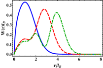
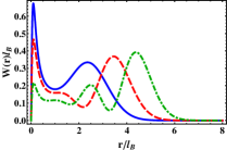
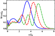
Figure 5: The radial functions of the electron density of the $m=0$ state for the Landau levels $n=0$ (blue solid lines), $n=-1$ (red dashed lines), and $n=-2$ (green dot-dashed lines) and three different values of the impurity charge: $\zeta=0.7$ (left panel), $\zeta=1.3$ (middle panel), $\zeta=1.9$ (right panel).

Further, the middle panel implies that the peak in the radial distribution function of the $n=0$ level near the impurity is redistributed among the $m=0$ states of the $n=-1,-2,...$ Landau levels. Obviously, this is an analog of the phenomenon of the diving into continuum for a supercritical charge in the absence of a magnetic field. In the latter case, the lowest bound state dives into the lower continuum producing a resonance whose wave function can be considered as redistributed over the lower continuum states with energies of the order of the resonance width $\gamma$. All wave functions from this region have an additional sharp peak near the origin. As we see, when magnetic field is present, there is a similar redistribution of the profiles of radial distribution functions near the impurity (note that as the impurity charge increases, the “redistribution” region shifts down to the lower Landau levels). According to the rightmost panel in Fig. 5, the blue curve representing the electron density is now similar to the red dashed curve in the leftmost panel and the red dashed curve is similar to the green dot-dashed curve in the leftmost panel.

So far we did not take into account the screening of a charged impurity due the polarization effects in graphene to which we turn our attention in the next subsection.

III.2 Tuning the screening of charged impurity with chemical potential

Experimentally, as shown in Sec. III.3, the strength of a charged impurity and splitting of Landau sublevels with different orbital momenta in a magnetic field can be very effectively tuned by a gate voltage Luican-Mayer2014 . In this subsection, we theoretically study this phenomenon by taking into account the polarization in a magnetic field which is controlled by the chemical potential due to gate voltage.

It is natural to attribute the variation in the strength of the impurity potential to the screening properties of the 2D electron system. To describe this effect theoretically, we follow Ref. [Sobol2016, ] and use the polarization function calculated in the absence of a charged impurity. Then the corresponding Poisson equation, which defines the screened impurity potential, reads

$$\sqrt{-\Delta_{2D}}V_{tot}(\mathbf{x})=-\frac{2\pi Ze^{2}}{\kappa}\delta^{(2)}(\mathbf{x})-\frac{2\pi e^{2}}{\kappa}\int\!\!d^{2}\mathbf{y}\Pi(\mathbf{x}-\mathbf{y};\mu)V_{tot}(\mathbf{y}),$$ (56)

where $\Pi(\mathbf{x}-\mathbf{y};\mu)$ is the static polarization function calculated by using the wave functions of free electrons in a magnetic field. Notice the presence of the pseudodifferential operator $\sqrt{-\Delta_{2D}}$ in the equation above, which is necessary to correctly describe the Coulomb interaction in a dimensionally reduced electrodynamic system Kovner1990 ; Dorey1992 ; Marino1993 ; Gorbar2001 .

Since Eq.(56) is algebraic in momentum space

$$\left(|\mathbf{q}|+\frac{2\pi e^{2}}{\kappa}\Pi(\mathbf{q};\mu)\right)V_{tot}(\mathbf{q})=-\frac{2\pi Ze^{2}}{\kappa},$$ (57)

we easily find the screened impurity potential in coordinate space

$$V_{tot}(\mathbf{x})=-\frac{Ze^{2}}{\kappa}\int\frac{d^{2}q}{2\pi}\frac{\exp(i\mathbf{q}\mathbf{r})}{|\mathbf{q}|+\frac{2\pi e^{2}}{\kappa}\Pi(\mathbf{q};\mu)}=-\frac{Ze^{2}}{\kappa}\int\limits_{0}^{+\infty}\!\!dq\frac{q\ J_{0}(q|\mathbf{x}|)}{q+\frac{2\pi e^{2}}{\kappa}\Pi(q;\mu)},$$ (58)

where $q=|\mathbf{q}|$. The static polarization function at zero temperature has the form Pyatkovskiy2011 ,

$$\Pi(q;\mu)=\frac{N_{f}}{4\pi l_{B}^{2}}\left\{\sum\limits_{n=0}^{n_{c}}\sum\limits_{\lambda=\pm}Q^{\lambda\lambda}_{nn}\left(\frac{q^{2}l^{2}_{B}}{2}\right)\delta_{\Gamma}(\mu-\lambda M_{n})-\underset{\lambda n\neq\lambda^{\prime}n^{\prime}}{\sum\limits_{n,n^{\prime}=0}^{n_{c}}\sum\limits_{\lambda,\lambda^{\prime}=\pm}}Q^{\lambda\lambda^{\prime}}_{nn^{\prime}}\left(\frac{q^{2}l^{2}_{B}}{2}\right)\frac{\theta_{\Gamma}(\mu-\lambda M_{n})-\theta_{\Gamma}(\mu-\lambda^{\prime}M_{n^{\prime}})}{\lambda M_{n}-\lambda^{\prime}M_{n^{\prime}}}\right\},$$ (59)

where $M_{n}=\frac{\hbar v_{\rm F}}{l_{B}}\sqrt{2n}$ are the Landau level energies, and we introduced the ultraviolet cutoff $n_{c}$ because of the divergence of the sum over the Landau levels. Since the bandwidth is finite in graphene, $n_{c}$ is estimated as $n_{c}=10^{4}/B[T]$ Roldan2009 ; Roldan2010 . As in experiment Luican-Mayer2014 , we consider the system of two superposed graphene layers twisted away from Bernal stacking by a large angle. This does not affect the spectrum of single-layer graphene but results in an additional twofold layer degeneracy: the factor $N_{f}=2_{s}2_{l}=4$ takes into account spin degeneracy and the presence of the second graphene layer. In experiment, this setup makes possible to diminish the random potential fluctuations due to substrate imperfections. The smeared delta function $\delta_{\Gamma}(x)=\frac{\Gamma}{\pi}\frac{1}{x^{2}+\Gamma^{2}}$ and the step function $\theta_{\Gamma}(x)=\frac{1}{2}+\frac{1}{\pi}\arctan\left(\frac{x}{\Gamma}\right)$ account for the finite width of Landau levels, and the functions $Q^{\lambda\lambda^{\prime}}_{nn^{\prime}}(y)$ are defined as

$$Q^{\lambda\lambda^{\prime}}_{nn^{\prime}}(y)=e^{-y}y^{|n-n^{\prime}|}\left(\sqrt{\frac{(1+\lambda\lambda^{\prime}\delta_{0,n_{>}})n_{<}!}{n_{>}!}}L^{|n-n^{\prime}|}_{n_{<}}(y)+\lambda\lambda^{\prime}(1-\delta_{0,n_{<}})\sqrt{\frac{(n_{<}-1)!}{(n_{>}-1)!}}L^{|n-n^{\prime}|}_{n_{<}-1}(y)\right)^{2},$$ (60)

where $n_{<}=\min(n,n^{\prime})$, $n_{>}=\max(n,n^{\prime})$ and $L_{n}^{m}(y)$ are the generalized Laguerre polynomials. The first term in Eq. (59) describes the contribution from the intralevel transitions while the second term represents the contribution from the interlevel transitions. For a small width of Landau levels the first term looks like a sequence of delta functions and contributes only when the chemical potential lies inside Landau levels. At small wave vectors ($q\ll l_{B}^{-1}$) the polarization function (59) behaves as Pyatkovskiy2011

$$\Pi(q;\mu)\simeq\frac{\kappa}{2\pi e^{2}}(q_{\text{TF}}+dq^{2}),$$ (61)

where

$$q_{\text{TF}}=\frac{e^{2}N_{f}}{\kappa l^{2}}\sum_{n=0}^{n_{c}}\sum_{\lambda=\pm}(2-\delta_{0n})\delta_{\Gamma}(\mu-\lambda M_{n})$$ (62)

is the Thomas-Fermi wave vector which determines the strength of the long-wavelength screening, and parameter $d$ is given by

$$d=-\frac{e^{2}N_{f}}{2\kappa}\sum_{n=0}^{n_{c}}\sum_{\lambda=\pm}(4n+\delta_{0n})\delta_{\Gamma}(\mu-\lambda M_{n})-\frac{e^{2}N_{f}l}{2\sqrt{2}\kappa\hbar v_{\rm F}}\sum_{n=0}^{n_{c}-1}\sum_{\lambda,\lambda^{\prime}=\pm}\frac{\theta_{\Gamma}(\mu-\lambda M_{n+1})-\theta_{\Gamma}(\mu-\lambda^{\prime}M_{n})}{(\lambda\sqrt{n+1}-\lambda^{\prime}\sqrt{n})^{3}}.$$ (63)

In fact, the static polarization function $\Pi(0,\mu)$ is proportional to the density of states which at finite scattering rate has the form of a series of broaden Landau levels Pyatkovskiy2011 . Figure 6 illustrates the dependence of the static polarization function (59) and its two leading long-wavelength terms (62) and (63) on the chemical potential. We plot for comparison the unscreened potential and the screened potential (58) of the impurity in Fig. 7. Let us consider the case where the chemical potential is situated between Landau levels. Then the Thomas-Fermi wave vector (62) is close to zero [Figs. 6(a) and 6(b)] and the Coulomb potential of the impurity is weakly screened, although even in this case graphene contributes to the total dielectric function at large and intermediate momenta, which effectively diminishes the charge of the impurity and the screened potential. Indeed, while the screened potential tends to its bare value at $r\to\infty$, it is weakened for small and intermediate distances (see the red dashed line in Fig. 7). On the other hand, when the chemical potential lies inside any given Landau level, the screening is much more effective due to large $q_{\text{TF}}$ (see the green dash-dotted line in Fig. 7) providing an excellent means of controlling the effective charge of impurity by the gate voltage which is directly related to the chemical potential $\mu$. Moreover, the coefficient $d$ in Eq. (63) in this case is negative [see Fig. 6(c)] which means that $\Pi(q;\mu)$ has a nonmonotonic momentum dependence with a peak at $q=0$. This behavior of the polarization function leads to the oscillations of the screened potential (green dash-dotted line in Fig. 7) with the sign change (i.e., the overscreening of the Coulomb potential) at intermediate distances of the order of several magnetic lengths.

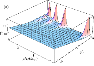
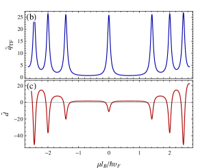
Figure 6: The dimensionless polarization function $\tilde{\Pi}=(4\pi\hbar v_{\rm F}l_{B}/N_{f})\Pi(q;\mu)$ as a function of the chemical potential and the wave vector (left panel) and the two coefficients $\tilde{q}_{\rm TF}=(2\kappa\hbar v_{\rm F}l_{B}/e^{2}N_{f})q_{\rm TF}$ and $\tilde{d}=(2\kappa\hbar v_{\rm F}/e^{2}N_{f}l_{B})d$ of its expansion (61) at small wave vectors (right panel).

Figure 7: The unscreened regularized Coulomb potential (blue solid line) and the screened potential of the impurity as a function of $r/l_{B}$ in the cases where the chemical potential is situated between Landau levels (red dashed line) and lies inside the zeroth Landau level (green dash-dotted line).

In Ref. [Sobol2016, ] the backreaction of the charged impurity on the polarization properties was also taken into account. Although the qualitative picture of screening is the same, it was shown that due to the downshift of the energy levels, the polarization function no longer remains symmetric with respect to the exchange $\mu\leftrightarrow-\mu$. These features of a charged impurity in graphene in the magnetic field are clearly observed in the recent experiments Luican-Mayer2014 ; Mao2016 .

It should be noted that the approximation of noninteracting electrons may become invalid when the chemical potential lies inside the Landau level. Indeed the electron-electron interactions could lead in sufficiently clean graphene specimen to such interesting phenomena as the fractional quantum Hall effect. Then, the chemical potential cannot be tuned continuously and instead jumps from one plateau to another. Although our analysis becomes inapplicable in the fractional quantum Hall regime, the experimental results in Luican-Mayer2014 show that the conclusion about the maximal screening remains unchanged.

III.3 Screening charged impurities and lifting the orbital degeneracy in graphene by populating Landau levels

Charged impurities in undoped gapless graphene produce a spatially localized signature in the density of states (DOS) which is readily observed with scanning tunneling microscope and spectroscopy (STM+STS)Mizes1989 . This effect is especially important in the presence of a magnetic field when the quantization of the 2D electronic spectrum into highly degenerate Landau levels (LL) gives rise to the quantum Hall effect. In this regime charged impurities are expected to lift the orbital degeneracy causing each LL in their immediate vicinity to split into discrete sublevels Gamayun2011 ; Zhang2012 .

By making use of high quality gated graphene devices in a magnetic field, it was shown in Ref.Luican-Mayer2014 that the strength of a charge impurity, as measured by its effect on the electron spectrum, can be effectively controlled by tuning the LL occupation with a back gate voltage. The LL spectra were obtained by measuring the bias voltage dependence of the differential tunneling conductance, $dI/dV$, which is proportional to the DOS, $D(E,\mathbf{r})$, at the tip position $\mathbf{r}$. Here $V=(E-E_{F})/e$ is the bias voltage and $E$ is the energy measured relative to the Fermi level, $E_{F}$. For almost empty LLs, the impurity is screened and essentially invisible whereas at full LL occupancy screening is very weak and the potential due to the impurity attains maximum strength. The underlying discrete quantum-mechanical spectrum arising from lifting the orbital degeneracy was experimentally resolved in the unscreened regime.

To explore the influence of the impurity on the LLs the spatial evolution of spectra along a trajectory traversing it for a series of gate voltages was studied. For certain gate voltages the spectra become significantly distorted close to the impurity, with the $n=0$ level (and to a lesser extent higher order levels) shifting downwards toward negative energies. The downshift indicates an attractive potential produced by a positively charged impurity. Its strength, as measured by the distortion of the $n=0$ LL, reveals a surprisingly strong dependence on LL filling. In the range of gate voltages $-15V<V_{g}<9V$ corresponding to filling the $n=0$ LL the distortion grows monotonically with filling. At small filling the distortion is almost absent indicating that the impurity is effectively screened attaining its maximum value close to full occupancy. At full occupancy the $n=0$ level shifts by as much as $\approx 0.1eV$ indicating that the effect would survive at room temperature. The spectral distortion is only present in the immediate vicinity of the impurity. Farther away no distortion is observed for all studied carrier densities.

The variation of the impurity strength with filling is related to the screening properties of the electron system. They were studied theoretically in Sec. III.2. For a positively (negatively) charged impurity and almost empty (full) LLs, unoccupied states necessary for virtual electron transitions are readily available in the vicinity of the impurity, resulting in substantial screening. By contrast for almost filled (empty) LLs, unoccupied states are scarce, which renders local screening inefficient.

The downshift is the largest for the $n=0$ and $j=-1/2$ state and diminishes with increasing $|j|$ and/or $n$. The local tunneling DOS was calculated in Ref.Luican-Mayer2014 assuming a finite linewidth $\Gamma$

$$D(E,\mathbf{r})=4\sum_{nj}\delta_{\Gamma}(E-E_{nj})\psi^{\dagger}_{nj}(\mathbf{r})\psi_{nj}(\mathbf{r}),$$ (64)

where $\delta_{\Gamma}(E-E_{nj})=\Gamma/[\pi((E-E_{nj})^{2}+\Gamma^{2})]$ represents a broadened LL. The peak intensity is determined by the probability density $\psi^{\dagger}_{nj}(\mathbf{r})\psi_{nj}(\mathbf{r})$ and is position dependent. If $\Gamma<\Delta{E_{nj}}$ ($\Delta E_{nj}$ defines spacing between adjacent levels), the discreteness of the spectrum is resolved, but for $\Gamma\geq\Delta{E_{nj}}$ the peaks of adjacent states overlap and merge into a continuous band.

Thus, even if the spectrum is discrete, but the resolution insufficient or if impurities are too close to each other, the measured $D(E,\mathbf{r})$ will still display “bent” LLs, whose energies seemingly adjust to the local potential. In particular, upon approaching the impurity the $n=0$ LL splits into well resolved discrete peaks connected with specific orbital states. As it could be seen from the experimental plots in Ref. [Luican-Mayer2014, ], the states $\psi_{0j}(\mathbf{r})$ with $j=-1/2,\,-3/2,\,-5/2$ are well resolved close to the impurity but higher order states are less affected and their contributions to $D(E,\mathbf{r})$ merge into a continuous line. Similarly, the discreteness of the spectrum is not resolved for $n\neq 0$ LLs that is consistent with the weaker impurity effect at larger distances. For partial filling ($V_{g}=-5\,{\rm V},0\,{\rm V}$) as screening becomes more efficient and orbital splitting is no longer observed, the unresolved sublevels merge into continuous lines of “bent” Landau levels. The ability to tune the strength of the impurity in-situ demonstrated in Ref.Luican-Mayer2014 opens the door to exploring Coulomb criticality and to investigate a hitherto inaccessible regime of criticality in the presence of a magnetic field Gamayun2011 ; Zhang2012 .

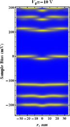
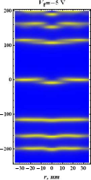
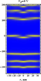
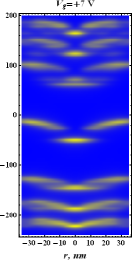
Figure 8: The local density of states calculated numerically in Ref. [Sobol2016, ] is plotted at four values of gate voltage along the line cuts across the impurity.

The tuning of the effective charge due to the polarization effects was studied theoretically by the three of us in Ref. [Sobol2016, ]. Numerically integrating the Dirac equation and determining the energies of several first Landau levels in the screened impurity potential (58), the local density of states along the line cuts across the impurity was determined and is plotted in Fig. 8. The corresponding LDOS is in good agreement with the experimental results of Ref. [Luican-Mayer2014, ] (see Fig.3 therein).

IV Two-electron bound states near a Coulomb impurity

In the weak interaction regime $\alpha\lesssim 0.4$, it was found in Ref. DeMartino2017 that a pair of repulsively interacting Dirac fermions in graphene in the attractive potential of a Coulomb impurity with charge $Ze$ forms a two-body bound state localized near the impurity. It could be observed by means of STM experiments similar to those previously reporting supercritical behavior in graphene Wang2012 ; Luican-Mayer2014 ; Wang2013 and trapped electron states in electrostatically defined graphene dots Lee2016 ; Gutierrez2016 .

The negatively charged two-electron hydrogen ion $H^{-}$ represents a classic problem of nonrelativistic quantum mechanics Chandrasekhar1944 ; Bethe1957 ; Hill1977 ; Bransden1983 ; Andersen2004 ; Hogaasen2010 . As it was shown in Ref. Hill1977 , there exists a single bound state in three spatial dimensions. Chandrasekhar proposed to construct a trial wave function for the ground state of $H^{-}$ as follows Chandrasekhar1944 :

$$\Psi({\bf r}_{1},{\bf r}_{2})=e^{-ar_{1}-br_{2}}-\epsilon e^{-br_{1}-ar_{2}},$$ (65)

where $r_{l}=|{\bf r}_{l}|$, $l=1,2$ denote the distance of the corresponding electron to the nucleus, $a$ and $b$ are the variational parameters, and $\epsilon=\mp 1$ corresponds to a spin singlet/triplet state, respectively. The variational calculation shows that the minimal energy for a two-body bound state is obtained for $a\neq b$ in the spin singlet configuration ($\epsilon=-1$).

The nonrelativistic 2D counterpart of the above system, which is the $D^{-}$ problem, describes a donor impurity ion with two electrons in a 2D semiconductor quantum well Phelps1983 ; Pang1990 ; Larsen1992a ; Larsen1992b ; Sandler1992 ; Ivanov2002 . The effects of quantum confinement on two-body bound-state energies have been studied experimentally in Ref. Huant1990 . In the absence of a magnetic field, there exists only a single bound state in the spin singlet sector. The $D^{-}$ problem is also similar to the negatively charged exciton ($X^{-}$) problem, which was experimentally studied in quantum wells Shields1995 .

The corresponding 2D relativistic problem could be realized in gapped graphene monolayers (or topological insulator surfaces) with a Coulomb impurity. However, it was found long ago that the relativistic $H^{-}$ problem is subtle because the single-particle Dirac Hamiltonian is unbounded from below Brown1951 ; Kolakowska1996 ; Nakatsuji2005 . In order to set a physically and mathematically well-posed problem, it is necessary to project the interaction Hamiltonian onto the states with positive energy. It can be devised for interacting Dirac fermions in graphene if (i) a single-particle gap exists ($\Delta>0$), and (ii) electron-electron interactions are weak, see Refs. Sucher1980 ; Sucher1984 ; Haeusler2009 ; Egger2010 .

We follow the derivation in Ref. [DeMartino2017, ] and consider the interacting two-particle problem for a gapped graphene monolayer in the presence of a charged impurity. The corresponding Dirac-Coulomb Hamiltonian at a given valley reads

$$H=\sum_{l=1,2}H(l)+V_{\rm 2b}.$$ (66)

Here $H(l)$ is the single-particle Dirac Hamiltonian (1) for particle $l=1,2$ with the single-particle potential of charge $Z$ impurity at the origin

$$V=-\frac{Ze^{2}}{\kappa r}=-\frac{Z\alpha_{g}\hbar v_{\rm F}}{\kappa r}$$ (67)

and $V_{\rm 2b}$ is the standard two-body Coulomb interaction which equals

$$V_{\rm 2b}=\frac{e^{2}}{\kappa|\mathbf{r}_{1}-\mathbf{r}_{2}|}.$$ (68)

However, as was mentioned above, the bound state problem is not well posed for the Dirac-Coulomb Hamiltonian of two particles (66) because the spectrum of the single-particle Dirac Hamiltonian is unbounded from below. A similar problem occurs in the study of relativistic effects in the helium atom as was found long ago by Brown and Ravenhall Brown1951 . According to Sucher Sucher1980 ; Sucher1984 , the Hamiltonian $H$ in Eq. (66) has to be replaced by the projected Hamiltonian Haeusler2009 ; Egger2010

$$H_{+}=H(1)+H(2)+\Lambda_{+}V_{\rm 2b}\Lambda_{+},$$ (69)

with the projection operator $\Lambda_{+}=\Lambda_{+}(1)\Lambda_{+}(2)$. Since $\mathcal{E}(l)=[H^{2}(l)]^{1/2}$ is positive definite, the single-particle operator $\Lambda_{+}(l)=\left[\mathcal{E}(l)+H(l)\right]/2\mathcal{E}(l)$, obviously, projects onto the positive energy states. As shown in Refs. Sucher1980 ; Sucher1984 ; Haeusler2009 ; Egger2010 , the projected Hamiltonian $H_{+}$ takes into account the most important effects of the electron-electron interaction. Further, due to the presence of a band gap, the replacement $H\to H_{+}$ is reliable for the ground state of the system in the limit of weak Coulomb repulsion. Moreover, the projection guarantees that the Hamiltonian $H_{+}$ can possess the genuine two-particle bound states.

Taking the two-particle wave function in a factorized form $\Phi_{\rm tot}=\Phi|\chi\rangle$, where $|\chi\rangle$ is the normalized spin part (singlet or triplet), its spatial part equals DeMartino2017

$$\Phi({\bf r}_{1},{\bf r}_{2})=\Psi_{I}({\bf r}_{1})\Psi_{O}({\bf r}_{2})-\epsilon\Psi_{O}({\bf r}_{1})\Psi_{I}({\bf r}_{2}),$$ (70)

where $\epsilon=\mp 1$ for the spin singlet/triplet sector and $\Psi_{I}$ and $\Psi_{O}$ are the normalized ground-state eigenspinors of the 2D relativistic hydrogen problem with charges $Z$ replaced by variational parameters $Z_{I}$ and $Z_{O}$. These eigenspinors are given by

$$\Psi_{\lambda}({\bf r})=\frac{p_{\lambda}}{\sqrt{\pi\Gamma(1+\gamma_{\lambda})}}\left(2p_{\lambda}r\right)^{(\gamma_{\lambda}-1)/2}e^{-p_{\lambda}r}\left(\begin{array}[]{l}\sqrt{1+\gamma_{\lambda}}\\ ie^{i\phi}\sqrt{1-\gamma_{\lambda}}\end{array}\right).$$ (71)

Here $\lambda=I,O$ and

$$\gamma_{\lambda}=\sqrt{1-4Z^{2}_{\lambda}\alpha^{2}},\qquad p_{\lambda}=2\Delta Z_{\lambda}\alpha/(\hbar v_{\rm F}).$$ (72)

For the energy functional

$$E_{\epsilon}(Z_{I},Z_{O})=\frac{\langle\Phi_{\rm tot}|H_{+}|\Phi_{\rm tot}\rangle}{\langle\Phi_{\rm tot}|\Phi_{\rm tot}\rangle}=\frac{\langle\Phi|H_{+}|\Phi\rangle}{\langle\Phi|\Phi\rangle},$$ (73)

calculating the matrix elements explicitly, we obtain the following energy functional (for details see Ref.DeMartino2017 ):

$$E_{\epsilon}(Z_{I},Z_{O})=\sum_{\lambda}\left(\Delta\gamma_{\lambda}+\frac{(Z_{\lambda}-Z)({\cal V}_{\lambda}-\epsilon S{\cal U})}{1-\epsilon S^{2}}\right)+\frac{{\cal V}^{\rm dir}_{\rm 2b}-\epsilon{\cal V}^{\rm exc}_{\rm 2b}}{1-\epsilon S^{2}},$$ (74)

where the overlap integral equals

$$S=\frac{\sqrt{(1+\gamma_{I})(1+\gamma_{O})}+\sqrt{(1-\gamma_{I})(1-\gamma_{O})}}{2}\frac{\Gamma(1+(\gamma_{I}+\gamma_{O})/2)}{\sqrt{\Gamma(1+\gamma_{I})\Gamma(1+\gamma_{O})}}\frac{(2p_{I})^{(1+\gamma_{I})/2}(2p_{O})^{(1+\gamma_{O})/2}}{(p_{I}+p_{O})^{1+(\gamma_{I}+\gamma_{O})/2}},$$ (75)

one-particle matrix elements are

$${\cal V}_{\lambda} = \langle\Psi_{\lambda}|(\alpha/r_{1})|\Psi_{\lambda}\rangle=2\alpha\frac{p_{\lambda}}{\gamma_{\lambda}},$$ (76)

$${\cal U} = \langle\Psi_{I}|(\alpha/r_{1})|\Psi_{O}\rangle=2\alpha\frac{p_{I}+p_{O}}{\gamma_{I}+\gamma_{O}}S,$$ (77)

and two-particle matrix elements

$${\cal V}_{\rm 2b}^{\rm dir} = \int d{\bf r}_{1}d{\bf r}_{2}\,\left|\Psi_{I}({\bf r}_{1})\right|^{2}\frac{\alpha}{r_{12}}\left|\Psi_{O}({\bf r}_{2})\right|^{2},$$ (78)

$${\cal V}^{\rm exc}_{\rm 2b} = \int d{\bf r}_{1}d{\bf r}_{2}\left[\Psi^{\dagger}_{I}({\bf r}_{1})\Psi_{O}({\bf r}_{1})\right]\frac{\alpha}{r_{12}}\left[\Psi^{\dagger}_{O}({\bf r}_{2})\Psi_{I}({\bf r}_{2})\right]$$ (79)

could be represented in terms of elliptic functions (see Ref. [DeMartino2017, ]).

It should be noted that the energy functional (74) includes the matrix elements of the full interaction operator rather than those of the projected operator, $\Lambda_{+}(\alpha/r_{12})\Lambda_{+}$, which are more difficult to obtain and would require a detailed numerical analysis. Both matrix elements coincide if the trial wave function has vanishing projection onto the negative energy eigenfunctions of $H_{\rm D}$. In fact, in Ref. [DeMartino2017, ], it was verified that for $\alpha\lesssim 0.4$ the cumulative weight of negative energy states in the trial wave function is very small ($\lesssim 1\%$). Indeed, negative energy states will only be important if typical interaction matrix elements can overcome the band gap $2\Delta$. For small $\alpha$, one therefore expects at most small quantitative corrections in the bound-state energy due to this approximation.

The energy functional (74) possesses the following features. First of all, it is symmetric under an exchange of its arguments. Second, for the spin-singlet case ($\epsilon=-1$), this energy is bounded from below for $Z\alpha<1/2$. Third, for small $\alpha$, $E_{\epsilon}(Z_{I},Z_{O})$ reduces to the corresponding nonrelativistic energy functional for the $D^{-}$ problem in 2D semiconductors Sandler1992 . However, in contrast to the nonrelativistic case, $E_{\epsilon}(Z_{I},Z_{O})$ is not homogeneous in $\alpha$, and hence the bound-state energy explicitly depends on $\alpha$. As in the nonrelativistic case, this energy minimum is realized for unequal values of $Z_{I}$ and $Z_{O}$.

It was shown in Ref. DeMartino2017 that the energy functional for the singlet state with $Z=1$ has a minimum located below the threshold, i.e., the binding energy is positive. In addition, there exists a two-body bound state. The situation is different in the spin triplet sector, where the variational approach predicts that the energy functional has a minimum whose energy is above the threshold and, thus, does not describe a bound state. For $Z=1$, the minimum is at $Z_{O}<1$ and $Z_{I}>1$ (or vice versa, due to the symmetry of $E_{\epsilon}$). Physically, one quasiparticle partially screens the impurity charge seen by the other quasiparticle.

Also in Ref. [DeMartino2017, ] the authors calculated the probability density and the pair distribution function for the bound state, focusing on the two-body spin singlet state. They suggest that the bound state can be accessed experimentally, e.g., by means of STM techniques.

V Two-center problem

Although, naively, the supercritical instability should be easily realized for charged impurities with $Z>1$, its experimental observation remained elusive due to the difficulty of producing highly charged impurities. However, one can reach the supercritical regime by collecting a large enough number of charged impurities in a certain region. As we saw in Sec. II.3, this approach was successfully realized by creating artificial nuclei (clusters of charged calcium dimers) on graphene Wang2013 using the tip of a scanning tunneling microscope. It is ironic that in spite of much larger value of coupling constant in graphene than in QED the first observation of the supercritical instability in graphene still required the creation of supercritical potentials from subcritical charges like in the case of heavy nuclei collisions in QED discussed in the Introduction. What crucially differs the graphene experiments Wang2013 from those in QED is that the supercritical electric fields created by placing together ionized Ca impurities are static unlike the fields created in heavy nuclei collisions in QED. This makes possible to observe and analyse reliably the supercritical regime.

The Hamiltonian of the two-center problem is the same as Hamiltonian (1) with the potential

$$V(\mathbf{r})=-\frac{e^{2}}{\kappa}\left(\frac{Z_{1}}{r_{1}}+\frac{Z_{2}}{r_{2}}\right),$$ (80)

where $r_{1,2}=|\mathbf{r}\pm\mathbf{R}/2|$ are the distances from electron to impurities with charges $Z_{1,2}$. Since the experiments in Ref. [Wang2013, ] were performed for impurities of the same type, we will study in what follows the symmetric problem, i.e., $Z_{1}=Z_{2}=Z$. The alignment of the charges with respect to the origin $r=0$ is arbitrary due to translational and rotational invariance of the free gapped Dirac Hamiltonian (1), and we choose them located at $(\mp R/2,0)$ with $R$ being a distance between two charges.

The main difficulty in solving the Dirac equation with two Coulomb centers in QED is that variables in this problem are not separable in any known orthogonal coordinate system Marinov1975 . Unfortunately, this is true also for the Dirac equation for two Coulomb centers in the $(2+1)$-dimensional problem in graphene. Therefore, we apply the approximate methods such as the linear combination of atomic orbitals (LCAO) technique and variational method.

V.1 LCAO approach for symmetric two-center problem

The LCAO method is well known and widely used in molecular physics Cohen-Tannoudji . Wave functions in this method are chosen as linear combinations of basis functions, where the latter are usually the electron functions centered on the corresponding atoms of the molecule. By minimizing the total energy of the system, the coefficients of the linear combinations are then determined. The LCAO approach for the symmetric two-center Dirac problem in 2D was applied in Ref.Klopfer2014 (see also Ref.Klopfer_thesis ), where only the lowest single-impurity bound state near each center is retained. This approximation is expected to yield accurate ground-state energies for large $R$ Matveev2000 ; Bondarchuk2007 , where the molecular ground state is well approximated in terms of atomic orbitals. In addition, as we show below, the exact result for $R\to 0$ is also captured by the LCAO solution.

For a single impurity of charge $Z$, the lowest bound state has the energy $\gamma\Delta$ with $\gamma=\sqrt{1-4Z^{2}\alpha^{2}}$. In the absence of short-distance regularization, the supercritical threshold is reached at $Z_{c}\alpha=1/2$ Gamayun2009 , therefore, $Z<Z_{c}$ is assumed henceforth. The corresponding normalized spinor, which is an eigenstate of the total angular momentum operator $J_{z}=-i\hbar\partial_{\phi}+\hbar\frac{\sigma_{z}}{2}$ with eigenvalue $1/2$, has the same form as (71) and reads

$$\Psi_{0}(r,\phi)=\frac{2Z\alpha}{\sqrt{\pi\Gamma(1+\gamma)}R_{\Delta}}\left(\frac{4Z\alpha r}{R_{\Delta}}\right)^{(\gamma-1)/2}e^{-2Z\alpha r/R_{\Delta}}\left(\begin{array}[]{c}\sqrt{1+\gamma}\\ ie^{i\phi}\sqrt{1-\gamma}\end{array}\right),$$ (81)

where $R_{\Delta}=\hbar v_{\rm F}/\Delta$.

It is convenient to rewrite the interaction potential as follows:

$$H=H_{0}-(Z_{\rm eff}+\delta Z)\frac{e^{2}}{\kappa}\left(\frac{1}{r_{1}}+\frac{1}{r_{2}}\right),$$ (82)

where $\delta Z=Z-Z_{\rm eff}$ and the effective charge $Z_{\rm eff}$ is introduced. It is a variational parameter, which could be determined by minimizing the total energy.

Following the standard LCAO approach Cohen-Tannoudji , we seek the electron wave function $|\Phi\rangle$ in terms of atomic orbitals, $|1\rangle$ and $|2\rangle$ centered near the Coulomb impurity at $(\mp R/2,0)$, which depend on $r_{1}$ and $r_{2}$, respectively, i.e., $|\Phi\rangle=v_{1}|1\rangle+v_{2}|2\rangle$. The atomic orbitals are chosen as eigenstates (81) in the field of a single impurity of charge $Z_{\rm eff}$. The Dirac equation is thereby reduced to a linear system of equations for $v_{1}$ and $v_{2}$, and the energy $E=E(Z_{\rm eff})$ follows from the condition

$${\rm det}\left(\begin{array}[]{cc}H_{11}-E&H_{12}-SE\\ H_{21}-SE&H_{22}-E\end{array}\right)=0,$$ (83)

where $H_{ij}=\langle i|H|j\rangle$ and the overlap integral $S=\langle 1|2\rangle=\langle 2|1\rangle$.

Defining the Coulomb integral,

$$C=\langle 1|r_{2}^{-1}|1\rangle=\langle 2|r^{-1}_{1}|2\rangle,$$ (84)

and the resonance integral,

$$A=\langle 1|r^{-1}_{1,2}|2\rangle=\langle 2|r_{1,2}^{-1}|1\rangle,$$ (85)

all matrix elements in Eq. (83) can be written in compact form:

$$H_{11} = H_{22}=\gamma\Delta-4Z_{\rm eff}\delta Z\alpha^{2}\Delta/\gamma-Z\frac{e^{2}}{\kappa}C,$$ (86)

$$H_{12} = H_{21}=\gamma S\Delta-(Z+\delta Z)\frac{e^{2}}{\kappa}A.$$

While $S$, $C$, and $A$ can be directly evaluated Matveev2000 ; Bondarchuk2007 in the 3D Dirac problem, the 2D case is, unfortunately, more involved. In order to compute them, it is useful to employ elliptic coordinates Gradshtein-book

$$\xi=\frac{r_{1}+r_{2}}{R}\in[1,\infty),\quad\eta=\frac{r_{1}-r_{2}}{R}\in[-1,1].$$ (87)

In these coordinates the integrals could be written as follows:

$$S = \frac{u^{\gamma+1}}{\pi\Gamma(1+\gamma)}\int_{1}^{\infty}d\xi\int_{-1}^{1}d\eta\frac{(\xi^{2}-\eta^{2})^{(\gamma-1)/2}e^{-u\xi}}{\sqrt{(\xi^{2}-1)(1-\eta^{2})}}\left[\xi^{2}-1+\gamma(1-\eta^{2})\right],$$ (88)

$$A = \frac{2u^{\gamma+1}}{\pi R\Gamma(1+\gamma)}\int_{1}^{\infty}d\xi\int_{-1}^{1}d\eta\frac{\xi(\xi^{2}-\eta^{2})^{(\gamma-3)/2}e^{-u\xi}}{\sqrt{(\xi^{2}-1)(1-\eta^{2})}}\left[\xi^{2}-1+\gamma(1-\eta^{2})\right],$$ (89)

$$C = \frac{2u^{\gamma+1}}{\pi R\Gamma(1+\gamma)}\int_{1}^{\infty}d\xi\int_{-1}^{1}d\eta\frac{(\xi+\eta)^{\gamma}e^{-u(\xi+\eta)}}{\sqrt{(\xi^{2}-1)(1-\eta^{2})}},$$ (90)

where $u=\frac{2RZ_{\rm eff}\alpha}{R_{\Delta}}$ and $\gamma=\sqrt{1-(2Z_{\rm eff}\alpha)^{2}}$.

Using the above integral representations for $S$, $C$, and $A$ (or the corresponding series from Ref. [Klopfer2014, ]), it is numerically straightforward to obtain an LCAO estimate for the ground-state energy $E(Z_{\rm eff})$ for given $Z_{\rm eff}$. Then the minimal energy is determined, realized for $Z_{\rm eff}=Z^{*}$, where the numerical search is aided by noting that $E(Z)$ depends quadratically on $Z_{\rm eff}-Z^{*}$. Numerical results in Ref. [Klopfer2014, ] show that the LCAO ground-state energy, $E(R)$, matches the expected single-impurity values $\gamma\Delta$ in both limits, namely (i) for $R\to\infty$ with impurity charge $Z$, where we have two decoupled copies of the single-impurity problem, and (ii) for $R\to 0$, where both centers conspire to form a single Coulomb impurity of charge $2Z$. Furthermore, it was shown that the optimal effective charge $Z^{*}$ nicely matches both limits as well.

Choosing larger $Z$ such that $\zeta=Z/Z_{c}=2Z\alpha$ is within the bounds $1/2<\zeta<1$, the supercritical regime can be realized by decreasing $R$ through a transition value, $R=R_{\rm cr}$. At the critical distance, the ground-state energy reaches the Dirac sea, $E(R_{\rm cr})=-\Delta,$ and for $R<R_{\rm cr}$, the two-center system with subcritical individual impurity charge becomes supercritical. The LCAO results in Ref. [Klopfer2014, ] show that, in practice, $Z$ has to be chosen quite close to $Z_{c}=1/(2\alpha)$, since otherwise $R_{\rm cr}$ becomes extremely small. This conclusion seems also in agreement with the reported experimental observations of supercriticality Wang2013 ; Luican-Mayer2014 , where different ions first had to be pushed closely together, thereby forming charged clusters, before supercriticality appears.

V.2 Variational method

Another means to study the supercritical instability of two Coulomb centers in graphene is the variational method which was applied to the corresponding two centers problem in QED in Ref. Marinov1975 . As noted in Ref. [Popov1972b, ], in order to obtain a satisfactory accuracy it is necessary that trial functions correctly reproduce the asymptotics of the exact solution at infinity and near the charged impurities. These asymptotics could be found from the direct analysis of the Dirac equation $\hat{H}\Psi=E\Psi$. For two-component spinor $\Psi(\mathbf{r})=(\phi,\ \chi)^{T}$, expressing $\chi$ in terms of $\phi$ leads to the following second order equation for the $\phi$ component of the Dirac spinor:

$$(\partial^{2}_{x}+\partial^{2}_{y})\phi+\frac{\frac{\partial V}{\partial x}-i\frac{\partial V}{\partial y}}{E-V+\Delta}\left(\frac{\partial\phi}{\partial x}+i\frac{\partial\phi}{\partial y}\right)+\frac{(E-V)^{2}-\Delta^{2}}{(\hbar v_{\rm F})^{2}}\phi=0.$$ (91)

According to Refs. [Zeldovich1972, ; Greiner1985, ], the supercritical instability takes place when the bound state with the lowest energy dives into the lower continuum. This occurs when $E=-\Delta$. For this solution, let us consider the asymptotic at large $r\gg R$, where the potential equals

$$V\left(\mathbf{r}\right)=-\zeta\hbar v_{\rm F}\left(\frac{1}{r}+\frac{R^{2}}{4r^{3}}P_{2}(\cos\varphi)+O\left(\frac{1}{r^{5}}\right)\right),$$ (92)

$\zeta=2Z\alpha$ is a dimensionless charge, and $P_{2}(x)$ is the Legendre polynomial $P_{n}(x)$ with $n=2$. In what follows we consider the case when charges of impurities are subcritical whereas their total charge exceeds a critical one, $1/2<\zeta<1$. The case $\zeta<1/2$ corresponds to the situation when the total charge is less than a critical one and is not relevant for the supercritical regime.

Neglecting the quadrupole and higher order multipole terms in the potential (this corresponds to the monopole approximation) Eq. (91) reduces to the following equation for $\phi(r)$:

$$\phi^{\prime\prime}+\frac{2}{r}\phi^{\prime}+\left(\frac{\zeta^{2}}{r^{2}}-\frac{2m\zeta}{r}\right)\phi=0,$$ (93)

where $m=\Delta/(\hbar v_{\rm F})$. The decreasing at infinity solution is expressed in terms of a Macdonald function,

$$\phi(r)=C_{1}r^{-1/2}K_{i\beta}(\sqrt{8m\zeta r}),\quad\beta=\sqrt{4\zeta^{2}-1}.$$ (94)

Its asymptotic

$$\phi_{\rm asym}(r)=C_{1}r^{-3/4}\exp(-\sqrt{8m\zeta r}),\quad r\to\infty$$ (95)

agrees, of course, with the asymptotical behavior of a solution to the Dirac equation of one center with charge $2Ze$. This shows also that the level which reached the boundary of the lower continuum remains localized.

In order to find the asymptotic of the solution in the vicinity of two Coulomb centers, it is conventional and convenient to use the elliptic coordinate system (87). We note that for charges of impurities such as $Z\alpha<1/2$ ($\zeta<1$) there is no “collapse” in the Coulomb field of one impurity Shytov2007a ; Shytov2007b ; Pereira2007 ; Gamayun2009 ; Khalilov2013 ; Chakraborty2013 ; Chakraborty2013a , therefore, it is not necessary to cut off the potential at small $r$ and the impurities may be considered as point-like. Therefore, for simplicity, in what follows, we will consider the nonregularized Coulomb potential. In elliptic coordinates, it has the form

$$V\left(\mathbf{r}\right)=-\frac{2\zeta\hbar v_{\rm F}\xi}{R(\xi^{2}-\eta^{2})}.$$ (96)

To find the asymptotic of $\phi$ in the vicinity of impurities, i.e., for small $\xi^{2}-\eta^{2}$, we seek $\phi$ in the form $\phi(\xi,\eta)=\phi(\mu)$, where $\mu=\xi^{2}-\eta^{2}=4r_{1}r_{2}/R^{2}$. Near the impurities $r_{1}\rightarrow 0$ or $r_{2}\rightarrow 0$, i.e., $\xi\rightarrow 1$ and $\eta\rightarrow\pm 1$ and, consequently, $\mu\to 0$, we obtain the following equation:

$$\frac{d^{2}\phi}{d\mu^{2}}+\frac{2}{\mu}\frac{d\phi}{d\mu}+\frac{\zeta^{2}}{4\mu^{2}}\phi=0,$$ (97)

whose regular solution at $\mu\to 0$ is

$$\phi_{\rm imp}(\mu)=C_{2}\mu^{-\sigma/2},\quad\sigma=1-\sqrt{1-\zeta^{2}}.$$ (98)

This asymptotic describes the behavior of the wave function at the impurities positions. Since at large distances $r\gg R$ the variable $\mu$ equals $\mu\simeq 4r^{2}/R^{2}$, solution (94) can be rewritten as follows:

$$\phi(\mu)=C_{1}\mu^{-1/4}K_{i\beta}(2\sqrt{m\zeta R}\mu^{1/4}).$$ (99)

Matching solutions (98) and (99) at the point $\mu=1$ we can find an approximate estimate of the critical distance $R_{\rm cr}(\zeta)$ as a function of $\zeta$. We obtain the following transcendental equation:

$$2\sqrt{1-\zeta^{2}}-1=2\sqrt{m\zeta R}\frac{K_{i\beta}^{\prime}(2\sqrt{m\zeta R})}{K_{i\beta}(2\sqrt{m\zeta R})}.$$ (100)

For $mR\ll 1$, i.e., when the distance between the impurities is much less than the Compton wavelength of quasiparticles, Eq. (100) can be simplified using the asymptotic of $K_{i\beta}(z)$ for $z\to 0$. Then we obtain the following analytical solution:

$$mR_{\rm cr}=\frac{1}{\zeta}\exp\left[-\frac{2}{\beta}\left(\cot^{-1}\frac{1-2\sqrt{1-\zeta^{2}}}{\beta}-{\rm arg}\Gamma(1+i\beta)\right)\right],$$ (101)

where $\Gamma(z)$ is the Euler gamma function. It is amazing that Eq. (101) coincides with the corresponding solution found in QED for scalar particles Popov1972 . Eq. (101) for $\sqrt{4\zeta^{2}-1}\ll 1$ can be written in more simple form

$$mR_{\rm cr}=\frac{1}{\zeta}\exp\left(-\frac{2\pi}{\sqrt{4\zeta^{2}-1}}\right).$$ (102)

We find that the deviation of $R_{\rm cr}$ given by Eq. (102) from that determined by Eq. (100) is rather small up to $\zeta=0.8$. A numerical calculation of $R_{\rm cr}$ given by these equations is presented in Fig. 9 in comparison with $R_{\rm cr}$ determined in more refined calculations using a variational method.

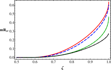
Figure 9: The dependence $mR_{\rm cr}(\zeta)$ given by Eqs. (100) (dash-dotted green line) and (101) (dash-dotted with two dots black line), and calculated by variational method with $N=1$ (blue dashed line) and $N=2$ (red solid line).

Clearly, the approximation we used is rather crude because it matches only the asymptotics and, in particular, it does not take into account at all the nonsphericity of the potential of two impurities described by $P_{2}(\cos\theta)$ and higher harmonics in potential (92).

To set up the variational problem, we note that the differential equation (91) can be obtained as an extremum of the following functional:

$$S[\phi]=\int\left((E-V+\Delta)^{-1}\left|\frac{\partial\phi}{\partial x}+i\frac{\partial\phi}{\partial y}\right|^{2}-\frac{(E-V-\Delta)}{(\hbar v_{\rm F})^{2}}|\phi|^{2}\right)dxdy,$$ (103)

under the condition that the norm $N=\int\Psi^{*}\Psi dxdy$ is conserved (this condition is important for obtaining the correct boundary conditions). Introducing a new field $\psi=W^{-1/2}\phi$, where $W=E-V+\Delta$, the functional $S[\phi]$ can be represented in the form specific for nonrelativistic quantum mechanics

$$S[\psi]=\int\left[|\bm{\nabla}\psi|^{2}+i\left(\frac{\bm{\nabla}V}{2W}\times\bm{\nabla}\psi^{*}\right)\psi-i\psi^{*}\left(\frac{\bm{\nabla}V}{2W}\times\bm{\nabla}\psi\right)+2(U-\epsilon)|\psi|^{2}\right]dxdy,$$ (104)

where $\mathbf{a}\times\mathbf{b}=\epsilon_{ij}a_{i}b_{j}$, $\epsilon=(E^{2}-\Delta^{2})/(2\hbar^{2}v_{\rm F}^{2})$ is the effective energy, and the effective potential $U$ is given by

$$U=\frac{2EV-V^{2}}{2(\hbar v_{\rm F})^{2}}+\frac{\triangle V}{4W}+\frac{3}{8}\frac{(\bm{\nabla}V)^{2}}{W^{2}}.$$ (105)

The second and third terms in functional (104) describe the pseudospin-orbit coupling with the field $\mathbf{F}=-{\bm{\nabla}V}/2W$, they do not contribute for the ground state wave function which is real. Functional (104) is bounded from below, so one is in position to apply to it the variational principle. In what follows we are interested in the case where the bound state with the lowest energy crosses the boundary of the lower continuum, so we put $E=-\Delta$ i.e., $\epsilon=0$. Then $W=-V$ and the functional $S[\psi]$ is simplified.

In QED, the Ritz and Kantorovich methods were employed in order to solve the variational problem and find a critical distance $R_{\rm cr}$ (see a discussion in Sec. III in Ref. [Popov-review2001, ]). In the Ritz method, the sought function $\psi$ is expanded over a fixed set of basis functions $\psi(x,y)=\sum_{n}c_{n}\psi_{n}(x,y)$, where $c_{n}$ are variational constants. In the Kantorovich method, $\psi=\sum_{n}c_{n}(x)\psi_{n}(y)$, where $\psi_{n}(y)$ are fixed functions, while $c_{n}(x)$ are variable functions. Obviously, the variational problem reduces to a system of linear algebraic equations for $c_{n}$ in the Ritz method and to a system of linear ordinary differential equations for $c_{n}(x)$ in the Kantorovich method.

According to Eq. (98), near impurities $\phi$ depends only on $\mu=\xi^{2}-\eta^{2}={4r_{1}r_{2}}/{R^{2}}$. At the large distances, $r\to\infty,$ the variable $\mu\to\infty$ and the asymptotic of $\phi$ is given by Eq. (99). Therefore, both asymptotics of $\psi$ depend only on $\mu$. In order that variational ansatz for $\psi$ give appropriate results, it is essential to take into account correctly the behavior of the exact solution near the Coulomb centers and at infinity. We choose the two variables $\mu,\nu$ so that the function $\psi(x,y)$ has a singularity only in $\mu$. Then using the following ansatz in the Kantorovich method:

$$\psi=\sum\limits_{k=1}^{N}\psi_{k}(\mu)\nu^{k-1},$$ (106)

where $\psi_{k}(\mu)$ are variable functions of $\mu$ and $\nu(\xi,\eta)$ is a fixed function of $\xi$ and $\eta$, we can maximally correctly take into account the behavior of the exact solution near the Coulomb centers. Since a priori we do not know what set of functions $\psi_{n}(x,y)$ is the best in the Ritz method, we use like in the QED studies Marinov1975 the Kantorovich method.

Two choices of function $\nu$ were considered in QED Marinov1975 : i) $\nu=\eta^{2}/(\xi^{2}-\eta^{2})=(r_{1}-r_{2})^{2}/4r_{1}r_{2}$ and ii) $\nu=\eta^{2}=(r_{1}-r_{2})^{2}/R^{2}$. The obtained results were close. Here, we will consider the case (i). Since the charges of impurities are identical, $Z_{1}=Z_{2}=Z$, the wave function of the ground state is symmetric under the inversion $x\rightarrow-x,y\rightarrow-y$, therefore, the change of the variables $x,y$ to $\mu,\nu$ is performed by means of the formulas

$$x=\frac{R}{2}\mu\sqrt{\nu(\nu+1)},\quad y=\frac{R}{2}[(\mu(\nu+1)-1)(1-\mu\nu)]^{1/2}.$$ (107)

Inserting ansatz (106) in Eq. (104) and integrating over $\nu$, we obtain

$$S_{N}(\psi)=4\sum\limits_{k,l=1}^{N}\int\limits_{0}^{\infty}d\mu\left(P_{kl}\psi_{k}^{\prime}{\psi^{*}_{l}}^{\prime}+Q_{kl}\psi_{k}\psi^{*}_{l}+R_{kl}\psi_{k}^{\prime}\psi^{*}_{l}+R_{kl}^{\dagger}{\psi_{k}}{\psi^{*}_{l}}^{\prime}\right),$$ (108)

where $P,Q$, and $R$ are $N\times N$ matrices which depend on $\mu$

$$P_{kl}(\mu)=\int\limits_{0}^{\infty}(\bm{\nabla}\mu)^{2}\nu^{k+l-2}|J|f(\mu,\nu)d\nu,$$ (109)

$$Q_{kl}(\mu)=\int\limits_{0}^{\infty}\Biggl{[}(\bm{\nabla}\nu)^{2}(l-1)(k-1)\nu^{k+l-4}-i(l-k)\left(\!\frac{\bm{\nabla}V}{2V}\times\bm{\nabla}\nu\!\right)\nu^{k+l-3}+2U\nu^{k+l-2}\Biggr{]}|J|f(\mu,\nu)d\nu,$$ (110)

$$R_{kl}(\mu)=\int\limits_{0}^{\infty}\Biggl{[}\bm{\nabla}\mu\bm{\nabla}\nu(l-1)\nu^{k+l-3}+i\left(\!\frac{\bm{\nabla}V}{2V}\times\bm{\nabla}\mu\!\right)\nu^{k+l-2}\Biggr{]}|J|f(\mu,\nu)d\nu.$$ (111)

Here $f(\mu,\nu)=\theta(1-\mu\nu)[\theta(1-\mu)\theta(\mu(\nu+1)-1)+\theta(\mu-1)]$, $|J|=\mu R^{2}/(16\sqrt{\nu(\nu+1)(\mu+\mu\nu-1)(1-\mu\nu)})$ is a Jacobian, $\bm{\nabla}$ is a gradient with respect to Cartesian coordinates, and $U$ is the effective potential. The explicit expressions for $\bm{\nabla}\mu$, $\bm{\nabla}\nu$, and $U$ are given in Appendix A in Ref. [Sobol2013, ].

Minima of functional (108) are given by solutions of the following set of Euler-Lagrange equations:

$$\frac{d}{d\mu}\left(P_{kl}\frac{d\psi_{k}}{d\mu}+R_{kl}^{\dagger}\psi_{k}\right)-Q_{kl}\psi_{k}-R_{kl}\frac{d\psi_{k}}{d\mu}=0.$$ (112)

The boundary conditions for functions $\psi_{k}$ follow from the requirement that the norm of the function $\psi$ be finite. The differential equation (112) and these boundary conditions define our boundary value problem.

In the simplest case $N=1$, we have

$$\frac{d}{d\mu}\left(P\frac{d\psi}{d\mu}\right)-Q\psi=0,$$ (113)

where $P(\mu)=\pi\mu$ and $Q(\mu)$ is expressed through the complete elliptic integrals of the first and second kind:

$$Q(\mu) = -\frac{\pi(\zeta^{2}-1)}{8\mu}\,+\frac{\zeta mR}{2}\left[\theta(1-\mu){\rm K}(\sqrt{\mu})+\frac{\theta(\mu-1)}{\sqrt{\mu}}{\rm K}\left(\!\frac{1}{\sqrt{\mu}}\!\right)\right]+$$ (114)

$$+ \theta(1-\mu)\biggl{[}\frac{3}{8\mu(1+\mu)}{\rm E}(\mu)-\frac{(2\zeta^{2}+1)(1+\mu)}{8\mu}{\rm K}(\mu)\biggr{]}+$$

$$+ \theta(\mu-1)\biggl{[}\frac{3}{8(1+\mu)}{\rm E}\left(\!\frac{1}{\mu}\!\right)-\frac{(\zeta^{2}-1)(1+\mu)+3\mu}{4\mu^{2}}{\rm K}\left(\!\frac{1}{\mu}\!\right)\!\biggr{]}.$$

We seek a wave function of the ground state which could be chosen real. Therefore, the function $R_{11}$, which is completely imaginary, does nor appear in Eq. (113).

The differential equation (113) determines the wave function of the critical bound state that just dives into the lower continuum. Since the wave function of a bound state tends to zero at infinity, this translates in our case to the condition $\psi(\mu)\to 0$ as $\mu\to\infty$. The asymptotic of the wave function near the impurities (where $\mu\to 0$) is given by Eq. (98). This equation completes the set-up of our boundary value problem which allows us to determine the critical distance $R_{\rm cr}$ between the impurities as a function of $\zeta$. Since the function $Q(\mu)$ is given in terms of the complete elliptic integrals of the first and second kind, the differential equation (113) cannot be solved analytically. We solve this equation numerically by using the shooting method and proceed as follows. We fix the wave function and its first derivative at certain small $\mu$ using Eq. (98). Then, we fix $\zeta$ and solve Eq. (113) numerically for different $mR$ [note that since the function $Q(\mu)$ depends only on the product $mR$, parameters $m$ and $R$ cannot be separately varied]. The critical distance $R_{\rm cr}$ (for a given $m$) is then determined as $R$ such that the wave function $\psi(\mu)$ tends to zero at infinity. Repeating this procedure for different $\zeta$, we find how the critical distance between the impurities depends on $\zeta$. The corresponding dependence $mR_{\rm cr}$ on $\zeta$ is plotted in Fig. 9 (blue dashed line).

The accuracy of computation can be improved taking $N>1$ in sum (106). In this case one should solve a set of second-order differential equations. Since the shooting method is not well suited for this purpose, it is better then to follow the corresponding calculations in QED in Ref. [Marinov1975b, ] and reduce the set of Eqs. (112) to a matrix Riccati equation, which can be solved by the Runge-Kutta method. The case $N=2$ was considered in Ref. [Sobol2014UJP, ] and the obtained results are quite close to the case $N=1$ and are shown in Fig. 9 (red solid line).

V.3 Quasistationary states

When the distance between the impurities becomes smaller than the critical one the bound state dives into the lower continuum transforming into a resonance. The energy and width of this quasistationary state could be determined using the Wentzel–Kramers–Brillouin method in the monopole approximation Sobol2013 . For distances $r>R$ (or more exactly $r\gg R$), the potential of the two-center problem is close to a spherically symmetrical one. Therefore, we can consider one charged impurity with the charge $2Ze$ and restrict our consideration only to the region $r\geq\varkappa R$, where $\varkappa\sim 1$ is a dimensionless constant. This is known as the monopole approximation.

For a spherically symmetric potential, the squared Dirac equation could be rewritten in the Schrödinger-like form (33) and the corresponding quasiclassical momentum $k(r,E)$ is given by Eqs. (34)–(36). To find the energy of quasibound states we use the Bohr–Sommerfeld quantization condition

$$\int\limits_{\varkappa R/2}^{r_{-}}k(r,E)dr=\int\limits_{\varkappa R_{\rm cr}/2}^{r_{-}^{0}}k(r,-\Delta)dr=2\pi\hbar n,$$ (115)

where $n=1,2...$ and $r_{-}$ is a boundary of the classically forbidden region determined by the equation $k(r_{\pm},E)=0$ and $r_{-}^{0}=r_{-}(E=-\Delta)$.

For energies close to the boundary of the lower continuum, $E\to-\Delta$, we find

$${E(R,\zeta)}=-{\Delta}\cdot F(\zeta,R),\quad\quad F(\zeta,R)=\left(\frac{R_{\rm cr}}{R}+\frac{1+2j}{4\zeta^{2}}-\frac{\zeta^{2}-j^{2}}{3\zeta^{2}}\right)/\left(1+\frac{1+2j}{4\zeta^{2}}-\frac{\zeta^{2}-j^{2}}{3\zeta^{2}}\right).$$ (116)

The width of quasistationary states apart from a preexponential factor is determined by tunneling through the classically forbidden region. For energies close to the boundary of the lower continuum, this gives the width

$$\Gamma\propto\exp\left[-2\pi\left(\zeta\sqrt{\frac{E^{2}}{E^{2}-\Delta^{2}}}-\sqrt{\zeta^{2}-j^{2}}\right)\right]\simeq\exp\left[-2\pi\left(\tilde{\beta}\sqrt{\frac{R}{R_{\rm cr}-R}}-\sqrt{\zeta^{2}-j^{2}}\right)\right],\tilde{\beta}=\sqrt{\frac{8\zeta^{2}+4j^{2}+6j+3}{24}},$$ (117)

which tends to zero when $E\to-\Delta$ or $R\to R_{\rm cr}$.

VI The dipole problem and migration of the wave function

The electron states for Dirac fermions in the field of two oppositely charged ($\pm Q$, $Q=Ze$) nuclei at distance $R$ ($ZeR$ is the corresponding electric dipole moment) in gapped graphene are described by Hamiltonian (1) with potential

$$V(\mathbf{r})=\frac{Ze^{2}}{\kappa}\left(\frac{1}{\sqrt{(x+R/2)^{2}+y^{2}}}-\frac{1}{\sqrt{(x-R/2)^{2}+y^{2}}}\right),$$ (118)

where $\kappa$ is the dielectric constant.

The corresponding Hamiltonian has an intrinsic particle-hole symmetry $\Omega\hat{H}\Omega^{+}=-\hat{H}$, where the unitary operator $\Omega=\sigma_{x}{\cal R}_{x}$ satisfies $\Omega^{2}=1$ (${\cal R}_{x}$ is the operator of reflection $x\to-x$). It follows then that an eigenstate $\Psi_{E}(x,y)$ with energy $E$ has a partner $\Psi_{-E}(x,y)=\Omega\Psi_{E}(x,y)=\sigma_{x}\Psi_{E}(-x,y)$ with energy $-E$, hence, all solutions of the Dirac equation come in pairs with $\pm E$.

This dipole problem was recently considered in Refs. [DeMartino2014, ; Klopfer2014, ] (the 3D Dirac equation with the electric dipole potential was also studied some time ago in Ref. [Matrasulov1999, ]). It was shown that the point electric dipole potential (this potential is defined as the limit $R\to 0$ of the finite-size electric dipole potential (118) with fixed electric dipole moment) accommodates towers of infinitely many bound states exhibiting a universal Efimov-like scaling hierarchy and at least one infinite tower of bound states exists for an arbitrary dipole strength. Notice that the Schrödinger equation in two dimensions for the electron in the field of an electric dipole also admits a bound state for any dipole strength Connolly2007 unlike the three-dimensional case where a bound state exists only when the dipole moment exceeds a certain critical value (see, e.g., a discussion including a historical one in Ref. [Turner1977, ]). By combining analytical and numerical methods, the authors of Ref. [DeMartino2014, ] found that the bound states do not dive into the lower continuum because the positive and negative energy levels first approach each other and then go away. Actually this behavior is typical for an avoided crossing Wigner1929 , which forbids level crossing for two states with the same quantum numbers. Since the bound states do not dive into the lower continuum, the authors of Ref. [DeMartino2014, ] concluded that supercriticality is unlikely to occur in the electric dipole problem in graphene.

We reconsidered the problem of supercriticality in our paper [Gorbar2015, ] for the case of two oppositely charged impurities situated at finite distance (finite-size electric dipole). By using the LCAO technique and variational Galerkin–Kantorovich method, we showed that for sufficiently large charges of impurities the wave function of the highest energy occupied bound state changes its localization from the negatively charged impurity to the positive one as the distance between the impurities changes (both methods gave similar results). The necessary condition for the instability to occur is the crossing of the electron energy levels in the field of single positively and negatively charged impurities. This migration of the electron wave function of the supercritical electric dipole is a generalization of the familiar phenomenon of the atomic collapse of a single charged impurity with holes emitted to infinity to the case where both electrons and holes are spontaneously created from the vacuum in bound states with two oppositely charged impurities thus partially screening them.

VI.1 Point electric dipole in graphene

Let us start from the case of $1/r^{2}$ point electric dipole potential, which was considered in Ref.DeMartino2014 . Far away from the nuclei, $r\gg R$, Eq. (118) is well approximated by the point-like dipole form

$$V_{d}(r,\theta)=-(\hbar v_{\rm F})^{2}\frac{p\cos\theta}{r^{2}},$$ (119)

where $p=ZRe^{2}/(\kappa\hbar^{2}v_{\rm F}^{2})$ is the quantity proportional to the effective electric dipole moment. The $r\to 0$ singularity requires regularization to avoid the usual fall-to-the-center problem, see below. For nonrelativistic Schrödinger fermions, the dipole captures bound states only above a finite critical dipole moment in three dimensions (3D) Abramov1972 ; Matrasulov1999 ; Camblong2001 ; Connolly2007 ; Schumayer2010 . However, a dipole binds states for arbitrarily small $p$ in the 2D Schrödinger case Connolly2007 .

The corresponding 3D Dirac electric dipole problem has not been discussed in (3+1)-dimensional QED presumably because of the lack of heavy anti-nuclei preventing its experimental realization in atomic physics. However, it could be directly studied using STM spectroscopy in graphene Wang2012 ; Luican-Mayer2014 ; Wang2013 . Bound states inside the gap, $E=\pm(\Delta-\varepsilon_{b})$ with binding energy $\varepsilon_{b}\ll\Delta$, come in ($j,\varkappa$) towers of definite “angular” quantum number, $j=0,1,2,\ldots$, and parity $\varkappa=\pm$ (with $j+\varkappa\geq 0$). The $(j,\varkappa)$ tower is only present if the dipole moment exceeds a critical value, $p>p_{j,\varkappa}$, but then contains infinitely many bound states. Since $p_{0,+}=0$, there is at least one such tower. Bound states in the same tower obey the scaling hierarchy

$$\frac{\varepsilon_{b,{n+1}}}{\varepsilon_{b,{n}}}=e^{-2\pi/s_{j,\varkappa}},\quad n=1,2,\ldots$$ (120)

where for $p$ close to (but above) $p_{j,\varkappa}$,

$$s_{j,\varkappa}(p)\simeq\left\{\begin{array}[]{ll}\sqrt{2}p\Delta,&(j,\varkappa)=(0,+),\\ \beta\sqrt{(p-p_{j,\varkappa})\Delta},&j>0,\end{array}\right.$$ (121)

with $\beta\approx 0.956$. Equation (120) agrees with the universal Efimov law for the binding energies of three identical bosons with short-ranged particle interactions Efimov1970 ; Braaten2006 ; Gogolin2008 . Numerical diagonalization of the Dirac equation in a finite disc geometry indicates that as $p$ increases, the bound states approach $E=0$ without ever reaching it. The absence of zero modes was shown analytically in Ref. DeMartino2014 .

For energies close to the band edge $E=-\Delta+\varepsilon_{b}$ with $|\varepsilon_{b}|\ll\Delta$, where $\varepsilon_{b}>0$ corresponds to bound states inside the gap and for $p\ll R^{2}\Delta/(\hbar v_{\rm F})^{2}$, the upper spinor component stays always “small”, $\phi\simeq\frac{\hbar v_{\rm F}}{2\Delta}e^{-i\theta}\left(i\partial_{r}+\frac{1}{r}\partial_{\theta}\right)\chi$. The equation, which determines the lower spinor component, has the form

$$\left(-\frac{(\hbar v_{\rm F})^{2}}{2\Delta}\nabla^{2}-V+\varepsilon_{b}\right)\chi=0,$$ (122)

with the 2D Laplacian $\nabla^{2}$. We proceed with the potential $V=V_{d}$ in Eq. (119), where Eq. (122) is solved by the ansatz $\chi(r,\theta)=F(r)Y(\theta)$. With separation constant $\gamma$, the angular function satisfies an $\varepsilon_{b}$-independent Mathieu equation,

$$\left(\frac{d^{2}}{d\theta^{2}}+\gamma-2p\Delta\cos\theta\right)Y(\theta)=0,$$ (123)

which admits $2\pi$-periodic solutions only for characteristic values $\gamma=\gamma_{j,\varkappa}(p)$, where $\varkappa=\pm$ is the parity, i.e., $Y_{j,\varkappa}(-\theta)=\varkappa Y_{j,\varkappa}(\theta)$, and due to the anisotropy, $j=0,1,2,\ldots$ differs from conventional angular momentum, with $j+\varkappa\geq 0$. Using standard notation Gradshtein-book ; AbramowitzStegun , the solutions to Eq. (123) are expressed in terms of Mathieu functions ${\rm ce}_{2j}$ and ${\rm se}_{2j}$, with eigenvalues $a_{2j}$ and $b_{2j}$, respectively,

$$Y_{j,+}(\theta) = {\rm ce}_{2j}\left(\frac{\theta}{2},4p\Delta\right),\quad\gamma_{j,+}=\frac{1}{4}a_{2j}(4p\Delta),$$ (124)

$$Y_{j,-}(\theta) = {\rm se}_{2j}\left(\frac{\theta}{2},4p\Delta\right),\quad\gamma_{j,-}=\frac{1}{4}b_{2j}(4p\Delta).$$

The characteristic values are ordered as $\gamma_{0,+}<\gamma_{1,-}<\gamma_{1,+}<\gamma_{2,-}<\ldots$ for given $p$. With $\gamma=\gamma_{j,\varkappa}(p)$, the radial equation reads

$$\left(\frac{d^{2}}{dr^{2}}+\frac{1}{r}\frac{d}{dr}-\frac{\gamma}{r^{2}}-2\frac{\Delta\varepsilon_{b}}{(\hbar v_{\rm F})^{2}}\right)F(r)=0.$$ (125)

To regularize the fall-to-the-center singularity, the Dirichlet condition $F(r_{0})=0$ is imposed at a short-distance scale $r_{0}\approx R$ (on the level of the Dirac equation, this corresponds to vanishing radial current at $r=r_{0}$). It is found that this regularization does not affect universal spectral properties such as the Efimov law (120).

Let us now look for bound states, $\varepsilon_{b}>0$. The solution of Eq. (125) decaying for $r\to\infty$ is the Macdonald function $K_{\sqrt{\gamma}}\left(\sqrt{2\Delta\varepsilon_{b}}\ r/(\hbar v_{\rm F})\right)$ Gradshtein-book , and the condition $F(r_{0})=0$ then yields an energy quantization condition within each ($j,\varkappa$) tower. Thereby the binding energies, $\varepsilon_{b,n,j,\varkappa}=z_{n}^{2}(\hbar v_{\rm F})^{2}/(2\Delta r_{0}^{2})$, are expressed in terms of the positive zeroes, $z_{1}>z_{2}>\ldots>0$, of $K_{\sqrt{\gamma_{j,\varkappa}}}(z)$. Since only $K_{is}(z)$ (with imaginary order) has zeroes Gradshtein-book , bound states require $\gamma_{j,\varkappa}(p)<0$. This condition is satisfied for $p>p_{j,\varkappa}$ with

$$\gamma_{j,\varkappa}\left(p_{j,\varkappa}\right)=0.$$ (126)

The lowest few $p_{j>0,\varkappa}$ resulting from Eq. (126) could be found in Ref. [DeMartino2014, ]. With increasing dipole moment, each time that $p$ hits a critical value $p_{j,\varkappa}$, a new infinite tower of bound states emerges from the continuum. Since $\gamma_{0,+}(p)<0$ for all $p$ AbramowitzStegun , we find $p_{0,+}=0$: at least one tower is always present. Explicit binding energies follow from the small-$z$ expansion of $K_{is}(z)$ Gradshtein-book . With the positive numbers $s_{j,\varkappa}(p)=\sqrt{-\gamma_{j,\varkappa}(p)}$ for $p>p_{j,\varkappa}$, see Eq. (121), we obtain

$$\varepsilon_{b,n,j,\varkappa}=\frac{2\hbar^{2}v_{\rm F}^{2}}{\Delta r_{0}^{2}}e^{\varphi(s_{j,\varkappa})}e^{-2\pi n/s_{j,\varkappa}},$$ (127)

where $\varphi(s)=(2/s)\ {\rm arg}\Gamma(1+is)$. This becomes more and more accurate as $n$ increases. For $n\to\infty$, in view of the particle-hole symmetry, the energies accumulate near both edges, $\varepsilon_{b,n}\to 0$. Importantly, Eq. (127) implies the Efimov scaling law announced in Eq. (120). This relation has its origin in the large-distance behavior of the dipole potential, and is thus expected to be independent of short-distance regularization issues. A similar behavior has been predicted for the quasi-stationary resonances of a supercritical Coulomb impurity in graphene Shytov2007a ; Gamayun2009 , and for 3D Schrödinger fermions Abramov1972 ; Schumayer2010 .

VI.2 Migration of the wave function in the finite dipole potential

In this subsection we consider the case of finite electric dipole with potential (118). Since the variables in Dirac equation with this potential are not separable in any orthogonal coordinate system, we will utilize the LCAO method. It is convenient to work with dimensionless quantities $h=H/\Delta$ and $\epsilon_{\Delta}=E/\Delta$ and use dimensionless coordinates and distances defined in units of $R_{\Delta}=\hbar v_{\rm F}/\Delta$. We use also dimensionless coupling constant $\zeta=Ze^{2}/(\hbar v_{\rm F}\kappa)$.

The LCAO method was used in Sec. V.1 to solve the two Coulomb centers problem in graphene. Here we apply LCAO method to the dipole problem in graphene. As to the atomic orbitals, we take the wave function of the lowest energy bound state in the field of positively charged impurity and the wave function of the highest energy bound state for negatively charged impurity (these wave functions are related to each other by charge conjugation).

We begin our analysis with the Dirac equation for the electron in graphene with one positively charged impurity $h_{p}\Psi_{p}=\epsilon_{\Delta}\Psi_{p}$ with the Hamiltonian

$$h_{p}=-i(\sigma_{x}\partial_{x}+\sigma_{y}\partial_{y})+\sigma_{z}-\frac{\zeta}{\sqrt{r^{2}+r_{0}^{2}}}.$$ (128)

[The Hamiltonian $h_{n}$ for the electron in the field of negatively charged impurity is obtained from the Hamiltonian $h_{p}$ by the change of the sign of the last term in $h_{p}$.]

We determine numerically the energy levels by using the shooting method with regular boundary conditions at $r=0$ for the wave functions and requiring that the wave functions decrease at infinity.

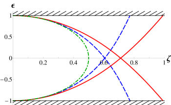
Figure 10: The energy of the electron bound state with $j=1/2$ in the regularized Coulomb potential with $\pm Ze$ charges as a function of $\zeta$ for different values of the regularization parameter: $r_{0}=0.05R_{\Delta}$ (red solid lines), $r_{0}=0.01R_{\Delta}$ (blue dashed lines), $r_{0}=0$ (green dash-dotted lines).

The energy of the lowest (highest) electron bound state with the total angular momentum $j=1/2$ in the regularized Coulomb potential with the charge $+Ze$ ($-Ze$) is plotted in fig.10 for different values of the regularization parameter $r_{0}$ as a function of $\zeta$. The levels which descend from the upper continuum correspond to the positive charge $+Ze$ while those which are pushed from the lower continuum and grow with $\zeta$ correspond to the negative charge $-Ze$. These results are in accordance with calculations in Ref.Gamayun2009 (see fig.4 there) where slightly different regularization for the one Coulomb center potential was used which admitted an analytical solution. They also reproduce qualitatively the behavior seen directly at the tight-binding level on a honeycomb lattice Pereira2008 . For nonregularized Coulomb potential with positive charge the lowest bound-state energy is always positive, it reaches the value $\epsilon=0$ for $\zeta=1/2$ and becomes purely imaginary for $\zeta>1/2$ (the fall-to-center phenomenon Shytov2007a ; Shytov2007b ; Pereira2007 ; Fogler2007 ). For regularized Coulomb potential with charge $+Ze(-Ze)$, the lowest (highest) bound-state energy crosses $\epsilon_{\Delta}=0$ and dives into the lower (upper) continuum at certain value of the charge. For example, for $r_{0}=0.05R_{\Delta}$, this happens for $\zeta\approx 1$.

Since the operator $U_{c}=\sigma_{x}K$ interchanges the $h_{p}$ and $h_{n}$ Hamiltonians, $U_{c}h_{p}U^{+}_{c}=-h_{n}$, the electron levels in the field of negatively charged center described by the Hamiltonian $h_{n}$ are obtained by the reflection $\epsilon_{\Delta}\rightarrow-\epsilon_{\Delta}$ and intersect with the levels of the Hamiltonian $h_{p}$ at $\epsilon_{\Delta}=0$. The corresponding critical value $\zeta_{c}$ when this happens will play a crucial role in the behavior of energy levels in the dipole potential because the behavior of these levels dramatically changes depending on whether $\zeta<\zeta_{c}$ or $\zeta>\zeta_{c}$. For chosen values of the regularization parameter $r_{0}$ in fig.10, the critical coupling $\zeta_{c}=0.6\,(r_{0}=0.01R_{\Delta})$ and $\zeta_{c}=0.7\,(r_{0}=0.05R_{\Delta})$. In general, $\zeta_{c}$ increases with the increase of $r_{0}$ (see Fig. 1 and Eq. (31)).

We are ready now to consider the Dirac equation for quasiparticles in graphene with two oppositely charged impurities. The corresponding Hamiltonian has the form

$$h=-i(\sigma_{x}\partial_{x}+\sigma_{y}\partial_{y})+\sigma_{z}+\frac{\zeta}{\sqrt{r_{n}^{2}+r_{0}^{2}}}-\frac{\zeta}{\sqrt{r_{p}^{2}+r_{0}^{2}}},$$ (129)

where $r_{p,n}=\sqrt{(x\pm R/2)^{2}+y^{2}}$. We seek the wave function as a linear combination (hybridization),

$$|\Psi\rangle=v_{p}|\Psi_{p}\rangle+v_{n}|\Psi_{n}\rangle,$$ (130)

of the wave functions $\Psi_{p}$ and $\Psi_{n}$ which are eigenstates of the Hamiltonians $h_{p}$ and $h_{n}$, respectively, with eigenvalues $\pm\epsilon_{0}$, and $\epsilon_{0}$ is the energy of the lowest-energy electron bound state in the field of one Coulomb center with the charge $+Ze$. Explicitly, the functions $|\Psi_{p}\rangle,|\Psi_{n}\rangle$ with the total angular momentum $j=1/2$ are given in polar coordinates by

$$\Psi_{p}=\left(\begin{array}[]{c}f(r_{p})\\ -ie^{i\theta_{p}}g(r_{p})\end{array}\right),\quad\Psi_{n}=\left(\begin{array}[]{c}e^{-i\theta_{n}}g(r_{n})\\ -if(r_{n})\end{array}\right),$$ (131)

where $\exp[-i\theta_{p,n}]=(x\pm R/2-iy)/r_{p,n}$. The radial functions $f(r)$ and $g(r)$ are computed numerically in the regularized potential of one positively charged impurity.

It is crucial for our analysis below to use the electron wave functions $|\Psi_{p}\rangle,|\Psi_{n}\rangle$ in the field of a single regularized Coulomb center whose energies may cross zero. By making use of the wave function (130), we project the Dirac equation $h|\Psi\rangle=\epsilon_{\Delta}|\Psi\rangle$ on the states $|\Psi_{p}\rangle$ and $|\Psi_{n}\rangle$ and find the following secular equation:

$$\det\left|\begin{array}[]{cc}h_{pp}-\epsilon_{\Delta}&h_{pn}-S\epsilon_{\Delta}\\ h_{np}-S\epsilon_{\Delta}&h_{nn}-\epsilon_{\Delta}\end{array}\right|=0,$$ (132)

where $h_{ij}=\langle i|h|j\rangle$, $\langle i|j\rangle=\delta_{ij}$, $i,j=\Psi_{p},\Psi_{n}$, $S=\langle\Psi_{p}|\Psi_{n}\rangle=\langle\Psi_{n}|\Psi_{p}\rangle$, $\langle\Psi|\Psi\rangle=1$. It is easy to see that the overlap integral

$$S=\int dxdy\left(f(r_{p})g(r_{n})\frac{x-R/2}{r_{p}}+f(r_{n})g(r_{p})\frac{x+R/2}{r_{n}}\right)$$

vanishes after changing $x\to-x$ in the first term of the brackets.

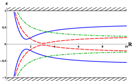
Figure 11: The energy of the bound state levels for $r_{0}=0.05R_{\Delta}$ as a function of distance in the LCAO method: $\zeta=0.65$ (green dash-dotted lines) and $\zeta=0.8$ (red dashed lines), $\zeta=0.9$ (blue solid lines).

In order to calculate the coefficients $h_{ij}$, it is convenient to represent the Hamiltonian in the form $h=h_{p}+{\zeta}/{\sqrt{r_{n}^{2}+r_{0}^{2}}}=h_{n}-{\zeta}/{\sqrt{r_{p}^{2}+r_{0}^{2}}}$. Then we obtain

$$h_{pp}=\epsilon_{0}+\langle\Psi_{p}|\frac{\zeta}{\sqrt{r_{n}^{2}+r_{0}^{2}}}|\Psi_{p}\rangle=\epsilon_{0}+\zeta C=-h_{nn},\quad h_{pn}=-\langle\Psi_{p}|\frac{\zeta}{\sqrt{r_{p}^{2}+r_{0}^{2}}}|\Psi_{n}\rangle=-\zeta A=h_{np}.$$ (133)

We find that the Coulomb integral $C$ equals

$$C=\langle p|\frac{1}{\sqrt{r_{n}^{2}+r_{0}^{2}}}|p\rangle=\int\limits_{0}^{\infty}\frac{4rdr}{\sqrt{(r+R)^{2}+r_{0}^{2}}}{\rm K}\left(\sqrt{\frac{4rR}{(r+R)^{2}+r_{0}^{2}}}\right)\left(f^{2}(r)+g^{2}(r)\right),$$ (134)

where ${\rm K}(k)$ is the complete elliptic integral of the first kind. We note that the Coulomb integral $C$ is positive definite and monotonously decreases with increasing $R$. Further, the resonance integral $A$ equals

$$A=\langle p|\frac{1}{\sqrt{r_{p}^{2}+r_{0}^{2}}}|n\rangle=2\int\limits_{-\infty}^{\infty}dx\int\limits_{0}^{\infty}dy\,f(r_{p})g(r_{n})\frac{x-R/2}{r_{n}}\left(\frac{1}{\sqrt{r_{p}^{2}+r_{0}^{2}}}-\frac{1}{\sqrt{r_{n}^{2}+r_{0}^{2}}}\right).$$ (135)

The Coulomb integral $C$ and resonance integral $A$ can be computed numerically with the functions $f$ and $g$ found for an isolated impurity problem. At small $R\sim 0$ we have that $C=const$ while $A\rightarrow 0$. Asymptotically at large $R$ they behave as $C\simeq 1/R$ and $A\sim\exp(-\sqrt{1-\epsilon_{0}^{2}}R)$.

Finally, we obtain the energy levels

$$\epsilon_{\Delta}=\pm\sqrt{(h_{pp})^{2}+(h_{pn})^{2}}=\pm\sqrt{(\epsilon_{0}+\zeta C)^{2}+\zeta^{2}A^{2}},$$ (136)

which are obviously symmetric with respect to the replacement $\epsilon_{\Delta}\to-\epsilon_{\Delta}$ in accord with the charge conjugation symmetry of the problem under consideration. We note that the energy levels never cross in agreement with the avoided crossing theorem Wigner1929 . Since the Coulomb and resonance integrals, $C$ and $A$, tend to zero as $R\rightarrow\infty$, the energy of the system for large distances between the impurities tends to $\epsilon_{\Delta}\rightarrow\pm|\epsilon_{0}|$ as expected. The coefficients of the wave function of the negative energy level are given by

$$v_{p} = -\frac{h_{pn}}{\sqrt{(h_{np})^{2}+(h_{pp}+\sqrt{(h_{pp})^{2}+(h_{pn})^{2}})^{2}}},$$ (137)

$$v_{n} = \frac{h_{pp}+\sqrt{(h_{pp})^{2}+(h_{pn})^{2}}}{\sqrt{(h_{np})^{2}+(h_{pp}+\sqrt{(h_{pp})^{2}+(h_{pn})^{2}})^{2}}}.$$ (138)

We plot the energy levels of the system for $r_{0}=0.05R_{\Delta}$ in Fig.11 as functions of $R$ for $\zeta=0.65$, $\zeta=0.8$ and $\zeta=0.9$. In the first case, we have $\zeta<\zeta_{c}=0.7$ and the bound state levels monotonously converge to each other as $R$ increases and never cross. For the couplings $\zeta=0.8$ and $\zeta=0.9$ which are larger than $\zeta_{c}=0.7$, their behavior is no longer monotonous. For small $R$, the levels converge like in the previous case. However, after the maximal convergence of the levels they go away with the subsequent increase of $R$. This behavior is typical for the avoided crossing Wigner1929 .

Eq.(136) and the facts that $C$ and $A$ monotonously depend on $R$ and $C\geq 0$ imply that the level repulsion can take place only for $\epsilon_{0}<0$ and the energy levels converge most closely for $\zeta C=|\epsilon_{0}|$ from which we can determine the corresponding distance $R_{m}$. Exactly at this distance $R_{m}$ we have $h_{pp}=h_{nn}=0$ from Eq.(133), hence $v_{p}=v_{n}=1/\sqrt{2}$ and, consequently, the probability to find the electron near the positively and negatively charged impurities is the same. Furthermore, for $\zeta C\approx|\epsilon_{0}|$, the difference of the coefficients $v_{p}$ and $v_{n}$ squared equals

$$v_{n}^{2}-v_{p}^{2}=\frac{2h_{pp}\left(h_{pp}+\sqrt{(h_{pp})^{2}+(h_{pn})^{2}}\right)}{(h_{np})^{2}+(h_{pp}+\sqrt{(h_{pp})^{2}+(h_{pn})^{2}})^{2}}\sim{\rm sign}(h_{pp})={\rm sign}(\epsilon_{0}+\zeta C).$$ (139)

The following qualitative picture appears for $\epsilon_{0}<0$. For small $R$, $h_{pn}=h_{np}\sim 0$, hence $|v_{n}|\gg|v_{p}|$ and, therefore, the electron wave function of the negative energy level in the LCAO method is localized mainly on the negatively charged impurity. Although this result seems to be counter-intuitive, it is quite natural. The point is that the energy spectrum of the system for $R=0$ is composed of the upper and lower continua. Since the chemical potential in neutral graphene is zero, the electron states of the lower continuum are occupied. For small $R$, the positively charged impurity produces electron bound states which descend from the upper continuum. Obviously, there are also charged conjugated states localized near the negatively charged impurity, which rise from the lower continuum as $R$ increases. These states are occupied for sufficiently small $R$. Since $|v_{n}|=|v_{p}|$ at the point of maximal convergence $R=R_{m}$, the probability to find the electron near the negatively and positively charged impurities is then equal. As the distance between impurities $R$ increases further, the difference of the square moduli (139) changes sign because the Coulomb integral $C$ decreases with increasing $R$. This means that the electron wave function changes its localization to the positively charged impurity. This change of the wave function localization (the relocalization or ”migration” effect) is explicitly shown in Fig.12 for $\zeta=0.85$ when $\epsilon_{0}=-0.453<0$. The value of $R_{m}$, in general, depends on $r_{0}$ and on the value of the coupling constant $\zeta$. As the coupling increases, $R_{m}$ decreases. A similar phenomenon of the change of localization of wave function takes place in the fission of quarkonium resonances consisting of the heavy quark and antiquark Greiner1985 .

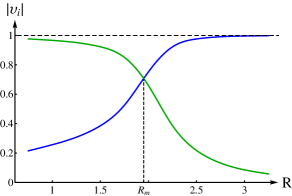
Figure 12: The dependence of coefficients (137)-(138) on the distance $R$ between the impurities for the negative-energy branch of the spectrum for $\zeta=0.85$: $|v_{p}|$ – decreasing line, $|v_{n}|$ – increasing line. The point of the change of localization $R_{m}$ is marked by dashed line.

It is clear that if $\epsilon_{0}>0$, then nothing interesting happens. Indeed, since $h_{pp}>0$ for $\epsilon_{0}>0$, we find that $|v_{n}|>|v_{p}|$ for any distance $R$ between the impurities. Therefore, the wave function is always localized on the negatively charged impurity and, consequently, the wave function of the highest occupied state does not change its localization. Note that the behavior of the energy levels in this case given by green dash-dotted lines in Fig.11 as a function of $R$ is monotonous unlike the case where $\epsilon_{0}$ is negative.

In Ref. Gorbar2015a we considered the numerical Galerkin–Kantorovich variational method and obtained qualitatively similar results.

VII Coulomb center problem in bilayer graphene

The Bernal stacked bilayer graphene forms a very interesting two-dimensional physical system whose electron excitations are described by the Hamiltonian with non-trivial chiral properties McCann2006 ; Novoselov2006 . These chiral fermions do not have analogues in high energy physics because their energy spectrum $E\sim\pm|\mathbf{p}|^{2}$ is parabolic in the two band model, like in non-relativistic systems described by the Schrödinger equation. Still since there are positive and negative energy bands related through the charge conjugation, this suggests that the instability connected with diving of the lowest energy electron bound state into the lower band may take place in gapped bilayer graphene too. In addition, it was shown in Ref. [Shytov-arXiv-2015, ] that the chirality of quasiparticles in gapless bilayer graphene results in cloaked bound states that do not hybridize with the hole continuum.

Actually, there is more to this. The parabolic spectrum in bilayer graphene is more soft than in monolayer graphene. Therefore, the electron-electron interactions are effectively enhanced and may open a gap connected with the condensation of electron-hole pairs in bilayer graphene. This conclusion agrees with the experimental data. While no gap is observed in monolayer graphene at the neutrality point, a small gap 2 meV is realized in bilayer graphene Martin2010 ; Weitz2010 ; Freitag2012 in the absence of external electromagnetic fields. A much larger gap ($\sim 42$ meV) is observed in high-mobility ABC-stacked trilayer graphene Lee2014 where electron excitations have a softer dispersion $E(\mathbf{p})\sim\pm|\mathbf{p}|^{3}$. As we mentioned above, the supercritical instability in the Coulomb center is a precursor of the excitonic instability and gap opening in the electron spectrum of a many-body problem. Reversing this argument and taking into account the fact that bilayer graphene is gapped due to the electron-electron interactions, one may expect that the supercritical instability for the electron in the field of Coulomb center should take place in bilayer graphene.

The following qualitative consideration is important for the analysis of the supercritical instability in bilayer graphene. Since the quasiparticle kinetic energy scales like $1/r^{2}$ with distance from the charged impurity in bilayer graphene and is negligible compared to the Coulomb interaction $1/r$, this suggests the absence of the critical charge for the formation of a bound state in this material. On the other hand, since the kinetic energy at small distances is larger than the Coulomb interaction energy, this implies that the fall-to-center should not take place in bilayer graphene. Therefore, a priori, one may expect that the supercritical instability in bilayer graphene should not be necessarily related to the phenomenon of the fall-to-center. The situation is different in monolayer graphene where both the kinetic energy and Coulomb interaction scale equally with distance. In fact, this equal scaling is the physical reason why the supercritical instability in monolayer graphene is related to the phenomenon of the fall-to-center where the electron wave function shrinks towards the impurity as its charge increases.

Clearly, the above heuristic reasoning is based on the scaling in the effective low-energy theory in bilayer graphene. However, the parabolic spectrum in bilayer graphene McCann2006 is valid only up to momenta $|\mathbf{p}|\approx\gamma_{1}/(2v_{\rm F})$, where $\gamma_{1}=0.39\,\mbox{eV}$ is the interlayer hopping amplitude. For larger momenta, the energy dispersion in linear as in the monolayer graphene. Therefore, it is possible, in principle, that as the charge of impurity increases the wave function of the electron bound state becomes more localized in the vicinity of the impurity such that the parabolic energy spectrum does not apply. If this happens, then the supercritical instability in bilayer graphene would proceed like in monolayer graphene and would be connected with the phenomenon of the fall-to-center. Actually, this scenario was advocated in Ref.[Kolomeisky2016, ], where it was argued by using the semiclassical approach that the supercritical instability is an“ultra-relativistic” effect in gapless bilayer graphene and, therefore, the value of the critical charge is the same as in monolayer graphene.

In order to see whether the supercritical instability is indeed related to the atomic collapse in bilayer graphene, the three of us studied in Ref. [Oriekhov2017, ] the electron bound states in the field of a charged impurity in bilayer graphene by using the two continuum models: the low-energy two-band model as well as the four-band model. The main principal advantage of the four-band model for the study of supercritical instability in bilayer graphene is that it takes into account the evolution of the electron energy dispersion from the low-energy quadratic to high energy linear energy dispersion. Since the trigonal warping is small in bilayer graphene, it could be neglected. On the other hand, the screening effects play a very essential role in view of the finite density of states at zero energy in bilayer graphene and should be taken into account. It will be shown that while the lowest energy bound state in the Coulomb center in gapped bilayer graphene indeed dives into the lower continuum, the wave function of the electron bound state does not shrink toward the impurity as its charge increases. This means that the supercritical instability in bilayer graphene is not related to the phenomenon of the fall-to-center.

VII.1 Two-band model

The two-band Hamiltonian, which describes low-energy electron excitations in gapped bilayer graphene in the field of an impurity with charge $Ze$, reads McCann2006

$$H=\frac{v^{2}_{F}}{\gamma_{1}}\left(\begin{array}[]{cc}0&(p_{-})^{2}\\ (p_{+})^{2}&0\end{array}\right)+\Delta\left(\begin{array}[]{cc}1&0\\ 0&-1\end{array}\right)+V(r),\quad V(r)=-\frac{Ze^{2}}{\kappa\,r},$$ (140)

where $p_{\pm}=p_{x}\pm ip_{y}$ and $\mathbf{p}=-i\hbar\bm{\nabla}$ is the two-dimensional momentum operator, $\gamma_{1}\approx 0.39\leavevmode\nobreak\ \mbox{eV}$ is the strongest interlayer coupling between pairs of orbitals that lie directly below and above each other, and $\kappa$ is the dielectric constant which we choose equal to 4 in our analysis.

The energy spectrum of the free part of Hamiltonian (140) is given by $E({\bf p})=\pm\sqrt{({\bf p}^{2}/2m^{*})^{2}+\Delta^{2}}$, so that we have a gap $2\Delta$ between the lower and upper continua (the valence and conductivity bands), where $m^{*}=\gamma_{1}/2v_{\rm F}^{2}\approx 0.054m_{e}$ is the quasiparticle mass and $m_{e}$ is the mass of the electron. Although the kinetic part of Hamiltonian (140) has the same matrix structure as in monolayer graphene leading to chirality and the particle-hole symmetry characteristic of relativistic systems, the dispersion relation for quasiparticles in bilayer graphene is quadratic like in non-relativistic systems. Thus, the low-energy Hamiltonian (140) non-trivially combines relativistic and non-relativistic properties. Clearly, while a regularized potential is crucially needed for the study of a charge instability in monolayer graphene, it suffices to use the standard potential $\sim 1/r$ for the two-band model of bilayer graphene with the parabolic dispersion of quasiparticles where the kinetic energy dominates over the potential one at small distance.

As we discussed in the Introduction and Sec.II, there is a critical charge of impurity in monolayer graphene above which the atomic collapse occurs. It is interesting what happens in bilayer graphene in view of the quadratic dispersion relation in this material. Although the two-band model is applicable only up to the energies of order $\gamma_{1}/4$ when the next band becomes important, it still makes sense to study how the supercritical Coulomb center instability is realized in the low-energy effective two-band model. We consider this problem in this section and discuss briefly the results obtained in the four-band model in the next subsection.

It is convenient to define the coupling constant as $\xi=\frac{Z\alpha_{g}}{\kappa}\sqrt{\frac{\gamma_{1}}{\Delta}}$ and express distances in terms of a characteristic length $\lambda_{\Delta}={\hbar v_{\rm F}}/{\sqrt{\gamma_{1}\Delta}}$ and wave vectors in its inverse, i.e., $\mathbf{\tilde{k}}=\mathbf{k}\,\lambda_{\Delta}$ (in what follows we will omit tilde over dimensionless momenta). The eigenstates of Hamiltonian (140) for $\Psi^{T}=(\chi,\varphi)$ are determined in momentum space by the following system of equations:

$$\left\{\begin{array}[]{c}{(k_{x}-ik_{y})^{2}\varphi\left(\mathbf{k}\right)}+{(1-\epsilon_{\Delta})\chi\left(\mathbf{k}\right)}+{\int\!\!\frac{d^{2}q}{(2\pi)^{2}}\,{{\chi{\left(\mathbf{q}\right)}}V_{\rm eff}\left(\mathbf{k}-\mathbf{q}\right)}}=0,\\ {(k_{x}+ik_{y})^{2}\chi\left(\mathbf{k}\right)}-{(1+\epsilon_{\Delta})\varphi\left(\mathbf{k}\right)}+{\int\!\!\frac{d^{2}q}{(2\pi)^{2}}\,{{\varphi{\left(\mathbf{q}\right)}}V_{\rm eff}\left(\mathbf{k}-\mathbf{q}\right)}}=0,\end{array}\right.$$ (141)

where $\epsilon_{\Delta}=E/\Delta$ and $V_{\rm eff}$ describes the screened potential of impurity with charge $Ze$. It is defined by an analog of the Poisson equation of the form

$$\sqrt{-\Delta_{2D}}V_{\rm eff}(\mathbf{x})=-2\pi\xi\delta^{(2)}(\mathbf{x})-\frac{4\pi\alpha_{g}}{\kappa}\int\!\!d^{2}\mathbf{y}\,\Pi(\mathbf{x}-\mathbf{y})V_{\rm eff}(\mathbf{y}),$$ (142)

where $\Pi(\mathbf{x})$ is the static polarization function in bilayer graphene. In momentum space, we easily find the following solution to Eq. (142):

$$V_{\rm eff}(q)=-\frac{2\pi\xi}{q+\frac{4\pi\alpha_{g}}{\kappa}\Pi(q)}\equiv-2\pi\xi\left(\frac{1}{q}-\delta V(q)\right),$$ (143)

where

$$\delta V(q)=\frac{4\pi\alpha_{g}}{\kappa}\frac{\Pi(q)}{q\left[q+\frac{4\pi\alpha_{g}}{\kappa}\Pi(q)\right]}$$ (144)

is the correction to the Coulomb interaction due to the screening effects. The one-loop polarization function as an integral over momentum was derived in Ref.[Nandkishore2010, ] and equals

$$\Pi(\mathbf{q})=\sqrt{\frac{\gamma_{1}}{\Delta}}\int\frac{d^{2}k}{(2\pi)^{2}}\frac{2(\epsilon_{-}\epsilon_{+}-1)-(\mathbf{k}-\frac{\mathbf{q}}{2})_{+}^{2}(\mathbf{k}+\frac{\mathbf{q}}{2})_{-}^{2}-(\mathbf{k}+\frac{\mathbf{q}}{2})_{+}^{2}(\mathbf{k}-\frac{\mathbf{q}}{2})_{-}^{2}}{\epsilon_{-}\epsilon_{+}(\epsilon_{-}+\epsilon_{+})},\quad\epsilon_{\pm}=\sqrt{1+\left|\mathbf{k}\pm\frac{\mathbf{q}}{2}\right|^{4}}.$$ (145)

For $q\ll 1$, the polarization function is proportional to $q^{2}$ and tends to zero for $q\to 0$, therefore, $\delta V(q)$ is not singular at $q=0$. For $q\gg 1$, $\Pi(q)=\sqrt{\gamma_{1}/\Delta}\ln 2/\pi$.

In polar coordinates, the angle and the absolute value of momentum variables can be separated. In order to do this, we note that the total $z$ component of the pseudospin-orbital momentum commutes with the Hamiltonian (140)

$$J_{z}=L_{z}+S_{z}=-i\hbar\frac{\partial}{\partial\theta}+\hbar\sigma_{z},\quad\quad[J_{z},\hat{H}]=0.$$ (146)

Thus, we seek the spinor function in the form

$$\Psi=\left(\begin{array}[]{c}\chi(\mathbf{k})\\ \varphi(\mathbf{k})\end{array}\right)=\left(\begin{array}[]{c}a_{j}(k)e^{i(j-1)\theta}\\ b_{j}(k)e^{i(j+1)\theta}\end{array}\right),$$ (147)

where $j$ is the total angular momentum which is integer in bilayer graphene. Substituting the spinor (147) into the system (141) and integrating over angle, we obtain

$$\left\{\begin{array}[]{c}k^{2}b_{j}(k)+a_{j}(k)-{\frac{\xi}{2\pi}}{\int\limits_{0}^{\Lambda}dqq\,a_{j}(q)[K_{j-1}(k,q)-\delta V_{j-1}(k,q)]}=\epsilon a_{j}(k),\\ k^{2}a_{j}(k)-b_{j}(k)-{\frac{\xi}{2\pi}}{\int\limits_{0}^{\Lambda}dqq\,b_{j}(q)[K_{j+1}(k,q)-\delta V_{j+1}(k,q)]}=\epsilon b_{j}(k),\end{array}\right.$$ (148)

where

$$K_{j}(k,q)=\int\limits_{0}^{2\pi}\frac{d\theta\cos(j\theta)}{\sqrt{k^{2}+q^{2}-2kq\cos\theta}}=\frac{2}{\sqrt{kq}}Q_{|j|-1/2}\left(\frac{k^{2}+q^{2}}{2kq}\right),$$ (149)

$$\delta V_{j}(k,q)=\int\limits_{0}^{2\pi}d\theta\,\delta V\left(\sqrt{k^{2}+q^{2}-2kq\cos\theta}\right)\,\cos(j\theta).$$ (150)

Here $Q_{\nu}(z)$ is the Legendre function of the second kind. The kernels $K_{j}(k,q)$ can be expressed in terms of the full elliptic integrals of the first and second kind. Unfortunately, it is not possible to find analytically a solution to the above system of equations. Its numerical solutions will be given in the next subsection. However, in Ref. [Oriekhov2017, ] the variational method was applied in order to have an analytic insight into the problem. It is based on the squared Schrödinger equation in coordinate space. The main result is that the critical charge of impurity $Z_{\rm cr}$ for the unscreened Coulomb potential tends to zero as $\sqrt{\Delta}$ as $\Delta\to 0$, while in the case of the screened interaction potential it tends to a finite value for $\Delta=0$.

VII.2 Numerical results

In order to find a numerical solution to the system of equations (148), we split the momentum interval $(0,\Lambda)$ in $N$ equal intervals and approximate the integrals by the sums of values of integrands at the ends of intervals multiplied by the weight function $w_{i}$ of the Newton-Cotes formula of the fifth order

$${\int\limits_{0}^{\Lambda}dqq[K_{j}(k,q)-\delta V_{j}(k,q)]b_{j}(q)}=\sum_{i=0}^{N}q_{i}w_{i}[K_{j}(k,q_{i})-\delta V_{j}(k,q_{i})]b_{j}(q_{i}).$$ (151)

The kernel $K_{j}(k,q)$ defined in Eq. (149) has a logarithmic singularity at $q=k$. In order to deal with this singularity, we use the following regularization for the first term in the square brackets on the left-hand side of Eq.(151):

$${\int\limits_{0}^{\Lambda}dqqK_{j}(k,q)b_{j}(q)}=\sum_{i=0}^{N}q_{i}w_{i}K_{j}(k,q_{i})[b_{j}(q_{i})-b_{j}(k)]+b_{j}(k){\int\limits_{0}^{\Lambda}dqqK_{j}(k,q)}.$$ (152)

The last integral in Eq.(152) is not singular and could be expressed through the elliptic integrals and generalized hypergeometric functions by using formulas from Sec. 5.11 in Ref.[Gradshtein-book, ]. For $j=0,1,2$, and $3$, the corresponding expressions are listed in Ref. [Oriekhov2017, ].

The quadrature step $h$ corresponds to the inverse of the size of a graphene disc, therefore, the energy spectrum of the system is discrete and the upper and lower continua existing in an infinite system appear now as the sets of closely situated discrete levels with the distance between them proportional to $h$. The energy levels of the corresponding upper and lower quasicontinua drift very slowly as the impurity charge increases. On the other hand, the bound levels inside the band gap shift towards the lower quasicontinuum much faster. Therefore, there exists a critical value of the impurity charge when the lowest energy bound state approaches the highest energy state of the lower quasicontinuum. We define this value as the critical charge. For different values of total angular momentum $j$, we find the different values of the critical charge (see the lower panel in Fig.14). The minimal value of the critical charge is obtained for $j=1$. Therefore, all numerical computations in this section are performed for this value of the total momentum.

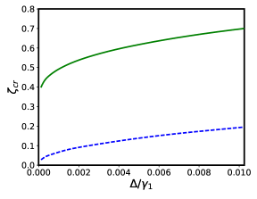
Figure 13: The critical coupling constant as a function of dimensionless gap $\Delta/\gamma_{1}$ with (green solid line) and without (blue dashed line) the screening effects taken into account.

The dependence of the critical coupling constant on gap $\Delta$ is plotted in Fig. 13 in the cases where the screening effects are absent and taken into account. Clearly, the critical charge decreases in both cases as gap decreases. According to our numerical calculations, the critical charge in the absence of the screening effects is very well approximated by the function $\zeta^{fit}_{cr}=1.88\sqrt{\Delta/\gamma_{1}}$. Such a gap dependence excellently agrees with the conclusion obtained from the variational method in Ref. [Oriekhov2017, ]. If the screening effects are taken into account, then the critical coupling constant does not tend to zero as $\Delta\to 0$. The results of the numerical solution to system (148) are quite similar to those obtained in Ref. [Oriekhov2017, ] by using the variational method and can be fit by the function

$$\zeta^{fit}_{cr}=0.36+4.32\sqrt{\Delta/\gamma_{1}}.$$ (153)

In order to quantify the localization properties of the wave function of the electron bound state in the near-critical regime and check the consistency of the use of the two-band model for the study of the supercritical instability in bilayer graphene, we plot for $Z\approx Z_{cr}$ in the right panel of Fig. 14 the square of the wave function in the two-band model in momentum representation $W(k)=2\pi k[a_{j}^{2}(k)+b_{j}^{2}(k)]/N$ multiplied by the weight factor $2\pi k$, where $N$ is the normalization constant $N=\int_{0}^{\Lambda}2\pi k[a_{j}^{2}(k)+b_{j}^{2}(k)]\,dk$. Obviously, if the wave function is localized in momentum space in the region of momenta $k\ll\Lambda$, then the use of the low-energy model for the description of the supercritical phenomena is consistent. According to the right panel in Fig. 14, the maximum of the wave function corresponds to $k\approx 0.075$. This value is 10 times less than the cutoff of the two-band model. This result suggests that the low-energy two-band model consistently describes the supercritical behavior in bilayer graphene.

Although our results show that the analysis of the supercritical instability is consistent in the two-band model, it is still necessary to study the supercritical instability in the four-band model of bilayer graphene. The point is that the quadratic energy dispersion in the two-band model is replaced by the linear energy dispersion as in monolayer graphene for momenta larger than $\gamma_{1}/(4v_{\rm F})$. Therefore, it is possible, in principle, that the supercritical instability will be affected by the electron dynamics at short distances. The four-band model whose energy dispersion smoothly interpolates between the low-energy quadratic and high-energy linear in momentum energy dispersion allows us to investigate whether the conclusions made in the present section survive in the four-band model.

In Ref. [Oriekhov2017, ] we studied the Coulomb center problem in bilayer graphene in the four-band model. The right panel of Fig. 14 compares the localization properties of the wave function of the electron bound state in the two- and four-band models. Clearly, the wave functions are localized in the same domain of momentum space in these models. This proves that the low-energy two-band model gives fairly accurate results for the Coulomb center problem in the case of small gaps.

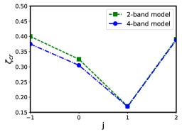
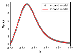
Figure 14: Left panel: The critical coupling constant as a function of total angular momentum $j$ for $\Delta=3$ meV. Right panel: The square of the wave function of the electron bound state for the near-critical charge $\zeta=\frac{Z\alpha_{g}}{\kappa}=0.17$ and the gap $\Delta=3$ meV are plotted for the two-band and four-band models as a function of dimensionless momentum, which is expressed in terms of $1/\lambda_{\gamma_{1}}$.

VIII Summary

In this review, we considered the electron states in the field of charged impurities in single layer graphene as well as bilayer graphene paying the special attention to the phenomenon of supercritical instability and its realization in the presence of several charged impurities and the external magnetic field. Such states are physically relevant for the actively developing area of graphene quantum dots whose shape and boundary conditions at edges strongly affect the confined states Peeters2017 . In addition, the electron states in the field of charged impurities are crucially important for the transport properties of graphene Rossi2011 .

In the supercritical Coulomb center problem, we showed that the “fall-to-center” phenomenon arises if $Z\alpha$ exceeds the critical value $1/2$ leading to the appearance of quasistationary levels with complex energies. The energy of quasistationary states in the case of gapless quasiparticles has a characteristic essential-singularity type dependence on the coupling constant reflecting the scale invariance of the Coulomb potential. It is found that a quasiparticle gap stabilizes the system decreasing the imaginary part $|{\Im m\,}E|$ of quasistationary states.

We reviewed also the experiments in which the supercritical behavior was observed. The STM measurements revealed the formation of resonances around artificial nuclei (clusters of charged calcium dimers) fabricated on gated graphene devices via atomic manipulation techniques. In a magnetic field, the STM and Landau level spectroscopy measurements demonstrate that the strength of the impurity can be tuned by controlling the occupation of Landau-level states with a gate-voltage. At low occupation the impurity is screened becoming essentially invisible. The screening of the potential of the impurity diminishes as states are filled until, for fully occupied Landau levels, the unscreened impurity significantly perturbs the spectrum in its vicinity. In this regime it is possible to observe the Landau-level splitting into discrete states due to lifting the orbital degeneracy.

Further, we studied theoretically the electron states in the field of a charged impurity in graphene in a magnetic field. The charged impurity removes the degeneracy of Landau levels converting them into band like structures. As the charge of impurity grows, the repulsion of sublevels of different Landau levels with the same value of orbital momentum takes place leading to the redistribution of the wave function profiles of these sublevels near the impurity Gamayun2011 ; Moldovan2017 . This qualitatively corresponds to the formation of resonance states in the traditional version of supercritical instability. Taking into account the polarization effects in a magnetic field allowed us to explain the tuning of the effective charge of the impurity by the gate voltage in agreement with the recent experiments.

In addition, the two-particle bound state problem for gapped graphene in the presence of a Coulomb impurity was studied. A variational approach, using the projected Hamiltonian and Chandrasekhar-Dirac spinors as trial wave functions, predicts the existence of at least one bound state. In contrast to the Schrödinger case, the variational energy functional is not a homogeneous function of the coupling constant $\alpha$. As a consequence, the optimal values of the variational parameters depend on $\alpha$ and the optimal binding energy has a more complicated functional dependence on $\alpha$. In particular, the binding energy increases with respect to the nonrelativistic case.

We studied also the supercritical instability in gapped graphene with two charged impurities separated by distance $R$ in the case where the charges of impurities are subcritical, whereas their total charge exceeds a critical one. The critical distance $R_{cr}$ in the system of two charged centers is defined as that at which the electron bound state with the lowest energy reaches the boundary of the lower continuum. Since the variables in the Dirac problem with two Coulomb centers are not separable in any known orthogonal coordinate system, this problem does not admit an analytic solution. Therefore, the critical distance $R_{cr}$ could be calculated only with the help of approximate methods. The LCAO technique and variational Kantorovich method give quite similar results. They show that the critical distance $R_{cr}$ increases as the quasiparticle gap decreases. The transition to the supercritical regime is signaled by the appearance of quasistationary states in the lower continuum.

A new type of supercritical behavior in gapped graphene with two oppositely charged impurities was revealed by studying the two-dimensional Dirac equation for quasiparticles with the Coulomb potential regularized at small distances. By utilizing the technique of linear combination of atomic orbitals and the variational Galerkin-Kantorovich method, it was shown that for supercritical electric dipole the wave function of the electron bound state changes its localization from the negatively charged impurity to the positively charged one as the distance between the impurities changes. Such a migration of the wave function corresponds to the electron and hole spontaneously created from the vacuum in bound states screening the positively and negatively charged impurities of the supercritical electric dipole, respectively. The obtained results were generalized in Ref.Gorbar2015a to a particle-hole asymmetric case, where the charges of impurities differ in signs and absolute values, and it was demonstrated that the necessary energetic condition for the supercriticality of novel type to occur is that the energy levels of single positively and negatively charged impurities traverse together the energy distance separating the upper and lower continua.

Finally, the supercritical instability in gapped bilayer graphene was studied in the low energy two-band as well as four-band continuum models. The different scalings of the kinetic energy of quasiparticles and the Coulomb interaction with respect to the distance to the charged impurity ensure that the wave function of the electron bound state does not shrink toward the impurity as its charge increases. This results in the absence of the fall-to-center phenomenon in bilayer graphene although the supercritical instability is realized. It was found that the screening effects are crucially important in bilayer graphene. If they are neglected, then the critical value for the impurity charge as the lowest energy bound state dives into the lower continuum tends to zero as the gap $\Delta$ vanishes. If the screened Coulomb interaction is considered, then the critical charge tends to a finite value when gap goes to zero.

- (1) L. Landau and E. Lifshitz, Quantum Mechanics. Non-relativistic Theory, Butterworth-Heinemann, Oxford, 2004.
- (2) I. Y. Pomeranchuk and Y. A. Smorodinsky, On energy levels in systems with , J. Phys. USSR 9, 97 (1945).
- (3) Y. B. Zeldovich and V. S. Popov, Electronic structure of superheavy atoms, Sov. Phys. Usp. 14, 673 (1972).
- (4) W. Greiner, B. Müller, and J. Rafelski, Quantum Electrodynamics of Strong Fields. With an Introduction into Modern Relativistic Quantum Mechanics, Texts and Monographs in Physics, Springer-Verlag, Berlin-Heidelberg, 1985.
- (5) S. S. Gershtein and Y. B. Zeldovich, Positron production during the mutual approach of heavy nuclei and the polarization of the vacuum, Sov. Phys. JETP 30, 358 (1970).
- (6) J. Rafelski, L. P. Fulcher, and W. Greiner, Superheavy Elements and an Upper Limit to the Electric Field Strength, Phys. Rev. Lett. 27, 958 (1971).
- (7) B. Müller, H. Peitz, J. Rafelski, and W. Greiner, Solution of the Dirac Equation for Strong External Fields, Phys. Rev. Lett. 28, 1235 (1972).
- (8) L. A. Fal’kovsky, Physical properties of bismuth, Sov. Phys. Usp. 11, 1 (1968).
- (9) V. S. Edel’man, Electrons in bismuth, Adv. Phys. 25, 555 (1976).
- (10) C. Herring, Accidental Degeneracy in the Energy Bands of Crystals, Phys. Rev. 52, 365 (1937).
- (11) N. P. Armitage, E. J. Mele, and A. Vishwanath, Weyl and Dirac Semimetals in Three Dimensional Solids, Rev. Mod. Phys. 90, 015001 (2018).
- (12) A. V. Shytov, M. I. Katsnelson, and L. S. Levitov, Atomic collapse and quasi-Rydberg states in graphene, Phys. Rev. Lett. 99, 246802 (2007).
- (13) A. V. Shytov, M. I. Katsnelson, and L. S. Levitov, Vacuum polarization and screening of supercritical impurities in graphene, Phys. Rev. Lett. 99, 236801 (2007).
- (14) V. M. Pereira, J. Nilsson, and A. H. Castro Neto, Coulomb Impurity Problem in Graphene, Phys. Rev. Lett. 99, 166802 (2007).
- (15) M. M. Fogler, D. S. Novikov, and B. I. Shklovskii, Screening of a hypercritical charge in graphene, Phys. Rev. B 76, 233402 (2007).
- (16) Y. Wang, D. Wong, A. V. Shytov, V. W. Brar, S. Choi, Q. Wu, H.-Z. Tsai, W. Regan, A. Zettl, R. K. Kawakami, S. G. Louie, L. S. Levitov, and M. F. Crommie, Observing atomic collapse resonances in artificial nuclei on graphene, Science 340, 734 (2013).
- (17) A. Feher, I. A. Gospodarev, V. I. Grishaev, K. V. Kravchenko, E. V. Manzhelii, E. S. Syrkin, and S. B. Feodos’ev, Effect of defects on the quasiparticle spectra of graphite and graphene, Low Temp. Phys. 35, 679 (2009) [Fiz. Nizk. Temp. 35, 862 (2009)].
- (18) V. M. Loktev and Y. G. Pogorelov, Impurity and vacancy effects in graphene, Low Temp. Phys. 38, 792 (2012) [Fiz. Nizk. Temp. 38, 993 (2012)].
- (19) Y. V. Skrypnyk and V. M. Loktev, Impurity induced Dirac point smearing in graphene, Low Temp. Phys. 33, 762 (2007) [Fiz. Nizk. Temp. 33, 1002 (2007)].
- (20) B. Dóra, Disorder effect on the density of states in Landau quantized graphene, Low Temp. Phys. 34, 801 (2008) [Fiz. Nizk. Temp. 34, 1020 (2008)].
- (21) O. V. Gamayun, E. V. Gorbar, and V. P. Gusynin, Supercritical Coulomb center and excitonic instability in graphene, Phys. Rev. B 80, 165429 (2009).
- (22) J. Wang, H. A. Fertig, and G. Murthy, Critical behavior in graphene with Coulomb interactions, Phys. Rev. Lett. 104, 186401 (2010).
- (23) J. Sabio, F. Sols, and F. Guinea, Two-body problem in graphene, Phys. Rev. B 81, 45428 (2010).
- (24) D. V. Khveshchenko, Ghost excitonic insulator transition in layered graphite, Phys. Rev. Lett. 87, 246802 (2001).
- (25) E. V. Gorbar, V. P. Gusynin, V. A. Miransky, and I. A. Shovkovy, Magnetic field driven metal-insulator phase transition in planar systems, Phys. Rev. B 66, 045108 (2002).
- (26) E. V. Gorbar, V. P. Gusynin, V. A. Miransky, and I. A. Shovkovy, Fractal structure of the effective action in (quasi)planar models with long-range interactions, Phys. Lett. A 313, 472 (2003).
- (27) D. V. Khveshchenko and H. Leal, Excitonic instability in layered degenerate semimetals, Nucl. Phys. B 687, 323 (2004).
- (28) O. V. Gamayun, E. V. Gorbar, and V. P. Gusynin, Gap generation and semimetal-insulator phase transition in graphene, Phys. Rev. B 81, 75429 (2010).
- (29) J. González, Electron self-energy effects on chiral symmetry breaking in graphene, Phys. Rev. B 85, 85420 (2012).
- (30) J. E. Drut and T. A. Lähde, Is graphene in vacuum an insulator?, Phys. Rev. Lett. 102, 026802 (2009).
- (31) J. E. Drut and T. A. Lähde, Critical exponents of the semimetal-insulator transition in graphene: A Monte Carlo study, Phys. Rev. B 79, 241405 (2009).
- (32) W. Armour, S. Hands, and C. Strouthos, Monte Carlo simulation of the semimetal-insulator phase transition in monolayer graphene, Phys. Rev. B 81, 125105 (2010).
- (33) P. V. Buividovich and M. I. Polikarpov, Monte Carlo study of the electron transport properties of monolayer graphene within the tight-binding model, Phys. Rev. B 86, 245117 (2012).
- (34) P. I. Fomin, V. P. Gusynin, V. A. Miransky, and Y. A. Sitenko, Dynamical symmetry breaking and particle mass generation in gauge field theories, Riv. Nuovo Cimento 6, 1 (1983).
- (35) R. D. Peccei, New phase for an old theory?, Nature 332, 492 (1988).
- (36) A. Luican-Mayer, M. Kharitonov, G. Li, C.-P. Lu, I. Skachko, A.-M. B. Gonçalves, K. Watanabe, T. Taniguchi, and E. Y. Andrei, Screening Charged Impurities and Lifting the Orbital Degeneracy in Graphene by Populating Landau Levels, Phys. Rev. Lett. 112, 036804 (2014).
- (37) J. Mao, Y. Jiang, D. Moldovan, G. Li, K. Watanabe, T. Taniguchi, M. R. Masir, F. M. Peeters, and E. Y. Andrei, Realization of a tunable artificial atom at a supercritically charged vacancy in graphene, Nat Phys 12, 545 (2016).
- (38) G. Giovannetti, P. A. Khomyakov, G. Brocks, P. J. Kelly, and J. van den Brink, Substrate-induced band gap in graphene on hexagonal boron nitride: Ab initio density functional calculations, Phys. Rev. B 76, 073103 (2007).
- (39) Y.-W. Son, M. L. Cohen, and S. G. Louie, Energy gaps in graphene nanoribbons, Phys. Rev. Lett. 97, 216803 (2006).
- (40) D. S. Novikov, Elastic scattering theory and transport in graphene, Phys. Rev. B 76, 245435 (2007).
- (41) V. M. Pereira, V. N. Kotov, and A. H. Castro Neto, Supercritical Coulomb impurities in gapped graphene, Phys. Rev. B 78, 085101 (2008).
- (42) I. S. Terekhov, A. I. Milstein, V. N. Kotov, and O. P. Sushkov, Screening of Coulomb Impurities in Graphene, Phys. Rev. Lett. 100, 076803 (2008).
- (43) A. Shytov, M. Rudner, N. Gu, M. Katsnelson, and L. Levitov, Atomic collapse, Lorentz boosts, Klein scattering, and other quantum-relativistic phenomena in graphene, Solid State Comm. 149, 1087 (2009).
- (44) A. H. Castro Neto, V. N. Kotov, J. Nilsson, V. M. Pereira, N. M. R. Peres, and B. Uchoa, Adatoms in graphene, Solid State Comm. 149, 1094 (2009).
- (45) C. G. Darwin, On some orbits of an electron, Philos. Mag. 25, 201 (1913).
- (46) I. S. Gradshtein and I. M. Ryzhik, Table of Integrals, Series, and Products, Academic, Orlando, FL, 1980.
- (47) V. R. Khalilov and C.-L. Ho, Dirac electron in a Coulomb field in (2+1) dimensions, Mod. Phys. Lett. A 13, 615 (1998).
- (48) P. Fomin, V. Gusynin, and V. Miransky, Vacuum instability of massless electrodynamics and the Gell-Mann-Low eigenvalue condition for the bare coupling constant, Phys. Lett. B 78, 136 (1978).
- (49) V. S. Popov, Position Production in a Coulomb Field with , Sov. Phys. JETP 32, 526 (1971).
- (50) P. Fomin and V. Miransky, On the dynamical vacuum rearrangement and the problem of fermion mass generation, Phys. Lett. B 64, 166 (1976).
- (51) Y. Wang, V. W. Brar, A. V. Shytov, Q. Wu, W. Regan, H.-Z. Tsai, A. Zettl, L. S. Levitov, and M. F. Crommie, Mapping Dirac quasiparticles near a single Coulomb impurity on graphene, Nat. Phys. 8, 653 (2012).
- (52) J. Li, W.-D. Schneider, and R. Berndt, Local density of states from spectroscopic scanning-tunneling-microscope images: Ag(111), Phys. Rev. B 56, 7656 (1997).
- (53) C. Wittneven, R. Dombrowski, M. Morgenstern, and R. Wiesendanger, Scattering States of Ionized Dopants Probed by Low Temperature Scanning Tunneling Spectroscopy, Phys. Rev. Lett. 81, 5616 (1998).
- (54) I. V. Krive and S. A. Naftulin, Dynamical symmetry breaking and phase transitions in a three-dimensional Gross-Neveu model in a strong magnetic field, Phys. Rev. D 46, 2737 (1992).
- (55) K. G. Klimenko, Three-dimensional Gross–Neveu model in an external magnetic field. I, Theor. Math. Phys. 89, 1161 (1991).
- (56) V. P. Gusynin, V. A. Miransky, and I. A. Shovkovy, Catalysis of Dynamical Flavor Symmetry Breaking by a Magnetic Field in 2 + 1 Dimensions, Phys. Rev. Lett. 73, 3499 (1994).
- (57) V. Gusynin, V. Miransky, and I. Shovkovy, Dimensional reduction and catalysis of dynamical symmetry breaking by a magnetic field, Nucl. Phys. B 462, 249 (1996).
- (58) E. V. Gorbar, V. P. Gusynin, V. A. Miransky, and I. A. Shovkovy, Coulomb interaction and magnetic catalysis in the quantum Hall effect in graphene, Phys. Scr. T146, 014018 (2012).
- (59) V. N. Oraevskii, A. I. Rex, and V. B. Semikoz, Spontaneous production of positrons by a Coulomb center in a homogeneous magnetic field, Sov. Phys. JETP 45, 428 (1977).
- (60) P. Schluter, G. Soff, K. H. Wietschorke, and W. Greiner, Bound electrons in critical magnetic fields, J. Phys. B: At. Molec. Phys. 18, 1685 (1985).
- (61) C.-L. Ho and V. R. Khalilov, Planar Dirac electron in Coulomb and magnetic fields, Phys. Rev. A 61, 32104 (2000).
- (62) O. V. Gamayun, E. V. Gorbar, and V. P. Gusynin, Magnetic field driven instability of a charged center in graphene, Phys. Rev. B 83, 235104 (2011).
- (63) T. Maier and H. Siedentop, Stability of impurities with Coulomb potential in graphene with homogeneous magnetic field, J. Math. Phys. 53, 095207 (2012).
- (64) S. C. Kim and S.-R. Eric Yang, Coulomb impurity problem of graphene in magnetic fields, Ann. Phys. 347, 21 (2014).
- (65) D. Moldovan, M. R. Masir, and F. M. Peeters, Magnetic field dependence of the atomic collapse state in graphene, 2D Materials 5, 015017 (2018).
- (66) G. W. Semenoff, I. A. Shovkovy, and L. C. R. Wijewardhana, Universality and the magnetic catalysis of chiral symmetry breaking, Phys. Rev. D 60, 105024 (1999).
- (67) O. O. Sobol, P. K. Pyatkovskiy, E. V. Gorbar, and V. P. Gusynin, Screening of a charged impurity in graphene in a magnetic field, Phys. Rev. B 94, 115409 (2016).
- (68) J. von Neumann and E. P. Wigner, Über das Verhalten von Eigenwerten bei adiabatischen Prozessen. (On the behavior of eigenvalues in the adiabatic processes.), Phys. Z. 30, 467 (1929).
- (69) B. Müller, J. Rafelski, and W. Greiner, Electron shells in over-critical external fields, Z. Phys. 257, 62 (1972).
- (70) A. Kovner and B. Rosenstein, Kosterlitz-Thouless mechanism of two-dimensional superconductivity, Phys. Rev. B 42, 4748 (1990).
- (71) N. Dorey and N. Mavromatos, QED3 and two-dimensional superconductivity without parity violation, Nucl. Phys. B 386, 614 (1992).
- (72) E. C. Marino, Quantum electrodynamics of particles on a plane and the Chern-Simons theory, Nucl. Phys. B 408, 551 (1993).
- (73) E. V. Gorbar, V. P. Gusynin, and V. A. Miransky, Dynamical chiral symmetry breaking on a brane in reduced QED, Phys. Rev. D 64, 105028 (2001).
- (74) P. K. Pyatkovskiy and V. P. Gusynin, Dynamical polarization of graphene in a magnetic field, Phys. Rev. B 83, 075422 (2011).
- (75) R. Roldán, J.-N. Fuchs, and M. O. Goerbig, Collective modes of doped graphene and a standard two-dimensional electron gas in a strong magnetic field: Linear magnetoplasmons versus magnetoexcitons, Phys. Rev. B 80, 085408 (2009).
- (76) R. Roldán, M. O. Goerbig, and J.-N. Fuchs, The magnetic field particle?hole excitation spectrum in doped graphene and in a standard two-dimensional electron gas, Semicond. Sci. Technol. 25, 034005 (2010).
- (77) H. A. Mizes and J. S. Foster, Long-Range Electronic Perturbations Caused by Defects Using Scanning Tunneling Microscopy, Science 244, 559 (1989).
- (78) Y. Zhang, Y. Barlas, and K. Yang, Coulomb impurity under magnetic field in graphene: A semiclassical approach, Phys. Rev. B 85, 165423 (2012).
- (79) A. De Martino and R. Egger, Two-electron bound states near a Coulomb impurity in gapped graphene, Phys. Rev. B 95, 085418 (2017).
- (80) J. Lee, D. Wong, J. Velasco Jr, J. F. Rodriguez-Nieva, S. Kahn, H.-Z. Tsai, T. Taniguchi, K. Watanabe, A. Zettl, F. Wang, L. S. Levitov, and M. F. Crommie, Imaging electrostatically confined Dirac fermions in graphene quantum dots, Nat. Phys. 12, 1032 (2016).
- (81) C. Gutiérrez, L. Brown, C.-J. Kim, J. Park, and A. N. Pasupathy, Klein tunnelling and electron trapping in nanometre-scale graphene quantum dots, Nat. Phys. 12, 1069 (2016).
- (82) S. Chandrasekhar, Some Remarks on the Negative Hydrogen Ion and its Absorption Coefficient, Astrophys. J. 100, 176 (1944).
- (83) H. A. Bethe and E. E. Salpeter, Quantum Mechanics of One- and Two-Electron Atoms, Academic Press, New York, 1957.
- (84) R. N. Hill, Proof that the ion has only one bound state. Details and extension to finite nuclear mass, J. Math. Phys. 18, 2316 (1977).
- (85) B. H. Bransden and C. J. Joachain, Physics of Atoms and Molecules, Longmont Group Limited, Hong Kong, 1983.
- (86) T. Andersen, Atomic negative ions: structure, dynamics and collisions, Phys. Rep. 394, 157 (2004).
- (87) H. Høgaasen, J.-M. Richard, and P. Sorba, Two-electron atoms, ions, and molecules, Am. J. Phys. 78, 86 (2010).
- (88) D. E. Phelps and K. K. Bajaj, Ground-state energy of a ion in two-dimensional semiconductors, Phys. Rev. B 27, 4883 (1983).
- (89) T. Pang and S. G. Louie, Negative-donor centers in semiconductors and quantum wells, Phys. Rev. Lett. 65, 1635 (1990).
- (90) D. M. Larsen and S. Y. McCann, Excited states of the two-dimensional center in magnetic fields, Phys. Rev. B 45, 3485 (1992).
- (91) D. M. Larsen and S. Y. McCann, Variational studies of two- and three-dimensional centers in magnetic fields, Phys. Rev. B 46, 3966 (1992).
- (92) N. P. Sandler and C. R. Proetto, Negative-donor centers in two dimensions, Phys. Rev. B 46, 7707 (1992).
- (93) M. V. Ivanov and P. Schmelcher, Two-dimensional negative donors in magnetic fields, Phys. Rev. B 65, 205313 (2002).
- (94) S. Huant, S. P. Najda, and B. Etienne, Two-dimensional centers, Phys. Rev. Lett. 65, 1486 (1990).
- (95) A. J. Shields, M. Pepper, M. Y. Simmons, and D. A. Ritchie, Spin-triplet negatively charged excitons in GaAs quantum wells, Phys. Rev. B 52, 7841 (1995).
- (96) G. E. Brown and D. G. Ravenhall, On the interaction of two electrons, Proc. Royal Soc. A 208, 552 (1951).
- (97) A. Kolakowska, J. D. Talman, and K. Aashamar, Minimax variational approach to the relativistic two-electron problem, Phys. Rev. A 53, 168 (1996).
- (98) H. Nakatsuji and H. Nakashima, Analytically Solving the Relativistic Dirac-Coulomb Equation for Atoms and Molecules, Phys. Rev. Lett. 95, 050407 (2005).
- (99) J. Sucher, Foundations of the relativistic theory of many-electron atoms, Phys. Rev. A 22, 348 (1980).
- (100) J. Sucher, Foundations of the relativistic theory of many-electron bound states, Int. J. Quantum Chem. 25, 3 (1984).
- (101) W. Häusler and R. Egger, Artificial atoms in interacting graphene quantum dots, Phys. Rev. B 80, 161402 (2009).
- (102) R. Egger, A. De Martino, H. Siedentop, and E. Stockmeyer, Multiparticle equations for interacting Dirac fermions in magnetically confined graphene quantum dots, J. Phys. A: Math. Theor. 43, 215202 (2010).
- (103) M. S. Marinov and V. S. Popov, Critical distance in collision of heavy ions, Sov. Phys. JETP 41, 205 (1975).
- (104) C. Cohen-Tannoudji, B. Diu, and F. Laloe, Quantum Mechanics, volume 2, Hermann, Paris, 1977.
- (105) D. Klöpfer, A. De Martino, D. Matrasulov, and R. Egger, Scattering theory and ground-state energy of Dirac fermions in graphene with two Coulomb impurities, Eur. Phys. J. B 87, 187 (2014).
- (106) D. Klöpfer, Critical Effects and Universality in Graphene Quantum Dots, PhD thesis, Düsseldorf, 2014.
- (107) V. I. Matveev, D. U. Matrasulov, and H. Y. Rakhimov, Two-center problem for the dirac equation, Phys. At. Nucl. 63, 318 (2000).
- (108) V. V. Bondarchuk, I. M. Shvab, D. I. Bondar, and A. V. Katernoga, Simple model of scalar-vector interaction for the relativistic two-center problem, Phys. Rev. A 76, 062507 (2007).
- (109) V. S. Popov, To the problem of the critical charge of nucleus, Sov. J. Nucl. Phys. 14, 257 (1972).
- (110) V. R. Khalilov, Zero-mass fermions in Coulomb and Aharonov-Bohm potentials in 2+1 dimensions, Theor. Math. Phys. 175, 637 (2013).
- (111) B. Chakraborty, K. S. Gupta, and S. Sen, Effect of topological defects and Coulomb charge on the low energy quantum dynamics of gapped graphene, J. Phys. A: Math. Theor. 46, 055303 (2013).
- (112) B. Chakraborty, K. S. Gupta, and S. Sen, Topology, cosmic strings and quantum dynamics – a case study with graphene, J. Phys. Conf. Series 442, 012017 (2013).
- (113) V. S. Popov, Critical charge in the two-center problem, JETP Lett. 16, 251 (1972).
- (114) V. S. Popov, Critical charge in quantum electrodynamics, Phys. At. Nucl. 64, 367 (2001).
- (115) M. S. Marinov, V. S. Popov, and V. S. Stolin, Variational approach to the relativistic two-center problem: Critical internuclear distance, J. Comput. Phys. 19, 241 (1975).
- (116) O. O. Sobol, Variational method for the calculation of critical distance between two Coulomb centers in graphene, Ukr. Jour. Phys. 59, 531 (2014).
- (117) O. O. Sobol, E. V. Gorbar, and V. P. Gusynin, Supercritical instability in graphene with two charged impurities, Phys. Rev. B 88, 205116 (2013).
- (118) A. De Martino, D. Klöpfer, D. Matrasulov, and R. Egger, Electric-dipole-induced universality for Dirac fermions in graphene, Phys. Rev. Lett. 112, 186603 (2014).
- (119) D. U. Matrasulov, V. I. Matveev, and M. M. Musakhanov, Eigenvalue problem for the relativistic electric-dipole system, Phys. Rev. A 60, 4140 (1999).
- (120) K. Connolly and D. J. Griffiths, Critical dipoles in one, two, and three dimensions, Am. J. Phys. 75, 524 (2007).
- (121) J. E. Turner, Minimum dipole moment required to bind an electron — molecular theorists rediscover phenomenon mentioned in Fermi-Teller paper twenty years earlier, Am. J. Phys 45, 758 (1977).
- (122) E. V. Gorbar, V. P. Gusynin, and O. O. Sobol, Supercritical electric dipole and migration of electron wave function in gapped graphene, Europhys. Lett. 111, 37003 (2015).
- (123) D. I. Abramov and I. V. Komarov, Weakly bound states of a charged particle in a finite-dipole field, Theor. Math. Phys. 13, 1090 (1972).
- (124) H. E. Camblong, L. N. Epele, H. Fanchiotti, and C. A. García Canal, Quantum Anomaly in Molecular Physics, Phys. Rev. Lett. 87, 220402 (2001).
- (125) D. Schumayer, B. P. van Zyl, R. K. Bhaduri, and D. A. W. Hutchinson, Geometric scaling in the spectrum of an electron captured by a stationary finite dipole, Europhys. Lett. 89, 13001 (2010).
- (126) V. Efimov, Energy levels arising from resonant two-body forces in a three-body system, Phys. Lett. B 33, 563 (1970).
- (127) E. Braaten and H.-W. Hammer, Universality in few-body systems with large scattering length, Phys. Rep. 428, 259 (2006).
- (128) A. O. Gogolin, C. Mora, and R. Egger, Analytical Solution of the Bosonic Three-Body Problem, Phys. Rev. Lett. 100, 140404 (2008).
- (129) M. Abramowitz and I. A. Stegun, Handbook of Mathematical Functions, Dover, New York, 1964.
- (130) E. V. Gorbar, V. P. Gusynin, and O. O. Sobol, Supercriticality of novel type induced by electric dipole in gapped graphene, Phys. Rev. B 92, 235417 (2015).
- (131) E. McCann and V. I. Fal’ko, Landau-level degeneracy and quantum Hall effect in a graphite bilayer, Phys. Rev. Lett. 96, 086805 (2006).
- (132) K. S. Novoselov, E. McCann, S. V. Morozov, V. I. Fal’ko, M. I. Katsnelson, U. Zeitler, D. Jiang, F. Schedin, and A. K. Geim, Unconventional quantum Hall effect and Berry/’s phase of in bilayer graphene, Nat. Phys. 2, 177 (2006).
- (133) A. V. Shytov, Cloaked resonant states in bilayer graphene, ArXiv [cond-mat.mes-hall] , 1506.02839 (2015).
- (134) J. Martin, B. E. Feldman, R. T. Weitz, M. T. Allen, and A. Yacoby, Local compressibility measurements of correlated states in suspended bilayer graphene, Phys. Rev. Lett. 105, 256806 (2010).
- (135) R. T. Weitz, M. T. Allen, B. E. Feldman, J. Martin, and A. Yacoby, Broken-symmetry states in doubly gated suspended bilayer graphene, Science 330, 812 (2010).
- (136) F. Freitag, J. Trbovic, M. Weiss, and C. Schönenberger, Spontaneously gapped ground state in suspended bilayer graphene, Phys. Rev. Lett. 108, 076602 (2012).
- (137) Y. Lee, D. Tran, K. Myhro, J. Velasco, N. Gillgren, C. N. Lau, Y. Barlas, J. M. Poumirol, D. Smirnov, and F. Guinea, Competition between spontaneous symmetry breaking and single-particle gaps in trilayer graphene, Nature Comm. 5, 5656 (2014).
- (138) E. B. Kolomeisky, J. P. Straley, and D. L. Abrams, Space charge and screening in bilayer graphene, J. Phys.: Cond. Mat. 28, 47LT01 (2016).
- (139) D. O. Oriekhov, O. O. Sobol, E. V. Gorbar, and V. P. Gusynin, Coulomb center instability in bilayer graphene, Phys. Rev. B 96, 165403 (2017).
- (140) R. Nandkishore and L. Levitov, Dynamical screening and excitonic instability in bilayer graphene, Phys. Rev. Lett. 104, 156803 (2010).
- (141) R. Van Pottelberge, M. Zarenia, P. Vasilopoulos, and F. M. Peeters, Graphene quantum dot with a Coulomb impurity: Subcritical and supercritical regime, Phys. Rev. B 95, 245410 (2017).
- (142) S. Das Sarma, S. Adam, E. H. Hwang, and E. Rossi, Electronic transport in two-dimensional graphene, Rev. Mod. Phys. 83, 407 (2011).