RESCEU-8/18

Long-term dynamics of cosmological axion strings

Masahiro Kawasaki,^a,b Toyokazu Sekiguchi,^c Masahide Yamaguchi^d

and Jun’ichi Yokoyama^b,c,e

^a ICRR, University of Tokyo, Kashiwa, 277-8582, Japan
^b Kavli Institute for the Physics and Mathematics of the Universe (Kavli IPMU), WPI, UTIAS, The University of Tokyo, Kashiwa, Chiba 277-8568, Japan
^c Research Center for the Early Universe (RESCEU), Graduate School of Science, The University of Tokyo, Tokyo 113-0033, Japan
^d Department of Physics, Tokyo Institute of Technology, 2-12-1 Ookayama, Meguro-ku, Tokyo 152-8551, Japan
^e Department of Physics, Graduate School of Science, The University of Tokyo, Tokyo 113-0033, Japan

We present results of new field-theoretic simulation of cosmological axion strings, which are eight times longer than previous ones. We have upgraded our simulation of physical strings in Hiramatsu et al. (2011) in terms of the number of grids as well as the suite of analysis methods. These improvements enable us to monitor a variety of quantities characterizing the dynamics of the physical string network for the longest term ever. Our extended simulations have revealed that global strings do not evolve according to the scaling solution but its scaling parameter, or the number of long strings per horizon, increases logarithmically in time. In addition, we have also found that the scaling parameter shows nontrivial dependence on the breaking scale of the Peccei-Quinn symmetry.

1 Introduction

The axion is one of the best motivated particles beyond the Standard Model [1, 2]. Its existence is inevitably derived from the Peccei-Quinn (PQ) mechanism [3], which dynamically solves the strong CP problem in quantum chromodynamics (QCD). Concurrently, it can account for the cold dark matter (CDM) in the observed Universe and offer rich phenomenology in the cosmological context (see e.g. [4, 5] for recent review). There are a few major production mechanisms of the axion CDM in the early Universe, including the misalignment and topological defects. A number of experiments are going on aiming at the detection of the CDM axion [6] (for review we refer to [7, 8, 9, 10]).

Formation of topological defects associated to the broken global PQ U(1) symmetry takes place if the symmetry breaking occurs after the observable Universe exits horizon during inflation. At first, axion strings form following the PQ phase transition. As the cosmological network of the strings evolves, its energy is released in the form of axion radiation. Later on, the QCD phase transition takes place and domain wall (DW) stretches out between the axion strings. If the number of DWs attached to each string is unity, the network of string-DW is unstable, so that it disappears soon after the QCD phase transition leaving additional contribution to the axion CDM [11]. Otherwise, DWs are stable and dominate the Universe, which spoils successful subsequent cosmology (see also [12]).

In this paper, we will focus on the network of axion strings in between the two phase transitions. This subject has already been studied by many different people for decades [13, 14, 15, 16, 17, 18, 19, 20, 21, 22, 23, 24, 25, 26]. However, the current picture of the string dynamics could not be developed straightforwardly. Notably, there had been long-standing controversies concerning, for instance, the number of strings per horizon and energy spectrum of radiated axions [13, 14, 15, 16, 17, 18, 19, 20, 21, 24]. Those controversies were settled principally with the aid of field theoretic simulation of the strings based on the first principles [21, 22, 23, 25, 26, 27, 28]. Nonetheless, as we shall reveal its novel dynamics in this Letter, axion strings seem still concealing its nature from us. We need to pursue better understanding of dynamics of global strings in order for accurate prediction of the axion CDM abundance.

The primary purpose of this paper is to update the result of our previous simulation [27]. In that paper, we performed field theoretic simulation of cosmological axion strings and estimated the relic abundance of axion radiated from the strings. Our simulation is improved mainly in two respects. Exploiting massively parallel computation on computer clusters, the number of grids is increased from $512^{3}$ to $4096^{3}$, which enhances the simulation time by a factor of eight. This allows us to examine long-term behavior of the string network. We also improved our analysis method. In [27], we introduced a novel string identification method and statistical reconstruction of the axion energy spectrum. In the present analysis, we incorporated estimation of velocity of strings and loop identification of strings in the suite of analysis. This allows us to monitor a variety of quantities characterizing the string network and examine its dynamics in detail.

This paper is organized as follows. In the next section, we will first describe the Lagrangian of the PQ scalar we simulate as well as the essence of our numerical simulation and analysis. Then in Section 3 we will present relevant results from our simulation. In particular, we pay particular attention to the long-term behavior of the string network, that is found in simulation of physical strings for the first time. The final section will be devoted to discussion.

2 Setup and analysis methods

2.1 Model

We adopt the following Lagrangian density for the PQ complex scalar $\Phi$ as in [26]:

$$\mathcal{L}=-|\partial_{\mu}\Phi|^{2}-V_{\rm eff}[\Phi;T],$$ (1)

where the effective potential $V_{\rm eff}[\Phi;T]$ is dependent on the temperature $T$:

$$V_{\mathrm{eff}}[\Phi;T]=\lambda(|\Phi|^{2}-v^{2})^{2}+\frac{\lambda}{3}T^{2}|\Phi|^{2},$$ (2)

with $v$ being the vacuum expectation value of $\Phi$ at $T=0$. The QCD axion $\varphi$ is identified as the phase of $\Phi$. At low energy, $\Phi$ can be written as $\Phi=\frac{f_{a}}{\sqrt{2}}e^{i\varphi/f_{a}}$, where $f_{a}=\sqrt{2}v$ is the decay constant of the axion. The mass of PQ field is also temperature dependent and given by $m^{2}(T)=\lambda(\frac{T^{2}}{3}-2v^{2})$. Given the potential, the PQ phase transition occurs at the critical temperature $T_{c}=\sqrt{6}v$. In what follows, quantities measured at $T=T_{c}$ are subscripted with $c$.

We assume a flat Universe with its line element given by

$$ds^{2}=-dt^{2}+a(t)^{2}d\bm{x}^{2}.$$ (3)

We normalize the scale factor at the PQ phase transition (i.e. $a_{c}=1$). We assume the radiation domination and the Hubble expansion rate $H$ is given by

$$H^{2}=\frac{\pi^{2}}{90}g_{*}\frac{T^{4}}{M_{*}^{2}},$$ (4)

where $g_{*}$ and $M_{*}$ are the relativistic degrees of freedom and the reduced Planck mass, respectively. Note that $t\propto a^{2}$ and the conformal time $\tau$ is given by $t/2a$ in the radiation domination. In what follows, we denote a derivative with respect to $t$ and $\tau$ with a dot and a prime (i.e. $\frac{\partial f}{\partial t}=\dot{f}$ and $\frac{\partial f}{\partial\tau}=f^{\prime}$), respectively.

Following [21], we adopt a parameter

$$\zeta=\left(\frac{45\lambda M_{*}^{2}}{2\pi^{2}g_{*}v^{2}}\right)^{1/2}.$$ (5)

Granting that the physical width of the axion string $d$ is given by $d\simeq(\sqrt{\lambda}v)^{-1}$, $\zeta$ parameterizes the ratio of the Hubble scale to the string width at the time of the PQ phase transition. In the following analysis, we fix $g_{*}=1000$ and $\lambda=1$ but vary $v$ among $v/M_{*}=0.005$, $0.002$ and $0.001$, which respectively give $\zeta=9.5$, $23.9$ and $47.8$.

2.2 Simulation

We start the simulation immediately before the PQ phase transition, and initial condition of the real and imaginary parts of the PQ field $\Phi=(\phi_{1}+i\phi_{2})/\sqrt{2}$ is generated assuming Gaussian random field with thermal distribution:

$$\langle\phi_{a}(\bm{x},t)\phi_{b}(\bm{y},t)\rangle = \frac{\delta_{ab}}{a^{3}}\int\frac{d^{3}k}{(2\pi)^{3}}\frac{1}{E_{\bm{k}}}\frac{1}{e^{E_{\bm{k}}/T}-1}e^{-i\bm{k}\cdot(\bm{x}-\bm{y})},$$ (6)

$$\langle\dot{\phi}_{a}(\bm{x},t)\dot{\phi}_{b}(\bm{y},t)\rangle = \frac{\delta_{ab}}{a^{3}}\int\frac{d^{3}k}{(2\pi)^{3}}\frac{E_{\bm{k}}}{e^{E_{\bm{k}}/T}-1}e^{-i\bm{k}\cdot(\bm{x}-\bm{y})},$$ (7)

$$\langle\phi_{a}(\bm{x},t)\dot{\phi}_{b}(\bm{y},t)\rangle = 0,$$ (8)

where $a,b=1,2$ and $E_{\bm{k}}=\sqrt{\frac{k^{2}}{a^{2}}+m^{2}}$.

We integrate the classical equation of motion of $\Phi$ using the leapfrog method. For detailed description of how the equation is discretized on the lattice, we refer readers to the appendices of [26]. The number of grids is $N_{g}=4096^{3}$, which is 512 times as large as in the previous simulations [27]. In order to suppress boundary effects, the size of the comoving simulation box $L$ is set to twice as large as the horizon scale at the final time (i.e. $L=\frac{2}{a_{f}H_{f}}$), where the subscript $f$ indicates the final time. The final time $t_{f}$ is determined by $t_{f}/d\simeq N_{g}^{1/3}/4\simeq 10^{3}$ so that the lattice spacing does not exceed the string width at $t_{f}$.

2.3 Analysis

We perform a suite of analysis in order to extract a variety of dynamical quantities associated to the string network. One of the essential techniques in the analysis is identification of axion strings from the discretized data of the PQ field on grids. We adopt the same string identification method as in [27], which tells us not only the existence of a string inside a given cell, but also its location in the cell if it does exist.

Furthermore, this time we introduce a novel method to identify string loops from the string points obtained from the string identification method. This is realized by grouping those string points by the Friends-of-Friends algorithm. We found that setting the physical linking length to $(d^{2}t)^{1/3}$ works in practice. Once a distinct loop is identified, we can compute its circumference length. By accumulating them we estimate the string parameter $\xi$, which is defined by

$$\rho_{\rm string}=\frac{\xi\mu}{t^{2}},$$ (9)

where $\mu$ is the tension of the axion string. The physical meaning of $\xi$ is the average number of strings per horizon volume.

We also implant an estimation method of string speed following [26]. On a point in the vicinity of a string, the string velocity can be estimated by

$$\bm{v}=\frac{(\nabla\Phi\times\nabla\Phi^{*})\times(\Phi^{\prime}\nabla\Phi^{*}-\Phi^{\prime*}\nabla\Phi)}{(\nabla\Phi\times\nabla\Phi^{*})^{2}}.$$ (10)

This is not exactly the same estimation method as in [26], but coincides when $\Phi$ vanishes on the point where we are trying to estimate the string velocity. Sometimes we found the magnitude of $\bm{v}$ exceeds unity. This failure of estimation is caused where a string has large curvature and/or strings are colliding. However, the fraction of the failure is at worst five percent and does not significantly bias the estimate of the rms of $\bm{v}$ that will be presented in the next section.

On the other hand, the energy spectrum of the axion radiation is computed according to the pseudo-power spectrum estimator [27]. The method consists mainly of two processes. First, we configure a window function which masks cells in proximity to string cores and compute the energy spectrum of axion convolved with the window function. Then we reconstruct the energy spectrum statistically by deconvolving the mode-mixing caused by the window function. This procedure can remove the contamination from the string cores, which dominates over the contribution genuinely from the axion radiation at high wave numbers.

More detailed description of our simulation and analysis will be presented in a separate paper [34].

3 Results

Figure 1 shows the time-evolution of the string parameter $\xi$ with $v/M_{*}=0.005$ (red open square), 0.002 (green open circle), and 0.001 (blue open circle). For reference, simulation result with the same setup as in our previous study [27] is also shown (red filled square), whose dynamic range is only as large as $t_{f}/d\simeq 40$. As can be read from the figure, $\xi$ grows in time and the time scale of the growth can be asymptotically characterized in $\ln(t/d)$. Although the magnitude of $\xi$ does not agree among $v/M_{*}=0.005$, $0.002$ and $0.001$, the asymptotic logarithmic growth is common. Such logarithmic growth has not been reported in the previous studies of physical strings including ours [27] due to the limitation of the dynamic range. Those simulations with such small dynamic range could trace the evolution only up to $t/d\lesssim\mathcal{O}(10)$ where such long-term dynamics has been buried in statistical uncertainties. The larger number of grids in our simulation, which enables longer duration of simulation, is essential in finding this novel property.

On the other hand, $\xi$ shown in Figure 1 incorporates both infinite strings and loops. Thus, one may wonder the logarithmic growth occurs only among loops or infinite strings. To answer this question, in Figure 2 we plot the string parameter only contributed from loops with length less than $t$ (left) and $\pi t$ (right). From the figure, one can see that the contribution of the loops in the total length is around 10 percent. Thus, the dominant contribution in $\xi$ comes from the infinite strings. In addition, the figure shows that the string parameter of loops does not apparently grow in time. Therefore, we conclude that the logarithmic growth seen in Figure 1 originates from the infinite strings.

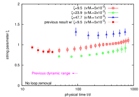
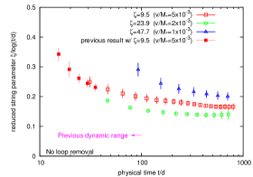
Figure 1: Evolution of string parameter $\xi$ (left) and $\xi/\log(t/d)$ (right). Shown are the cases with three different $v/M_{*}=0.005$ (red open square), $v/M_{*}=0.003$ (green open circle), and $v/M_{*}=0.001$ (blue open circle). For reference, we plotted the result of simulation corresponding to our previous study [27] (red filled square). Error bar shows the standard deviation among realizations. Magenta arrow shows the dynamic range that should have been available in the previous simulation [27].

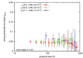
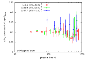
Figure 2: Evolution of string parameter contributed only from the loops with physical circumference length less than $t$ (left) and $\pi t$ (right). Color and symbol are the same as in Figure 1.

Velocity of strings also exhibits some degree of discrepancy from the previous studies. The root mean square of string velocity $\sqrt{\langle\bm{v}^{2}\rangle}$ is plotted in Figure 3. We found $0.6\lesssim\sqrt{\langle\bm{v}^{2}\rangle}\lesssim 0.7$ around the initial stage, which is consistent with [26]. However, as time advances, it decreases gradually and reads around 0.5 at the later time of the simulation. This is substantially smaller compared to the velocity estimated from simulation of local-string based on the Nambu-Goto action [29, 30] but consistent with field-theoretic simulation of local strings [31]. At this moment, we are unable to tell if the velocity has settled down already within the simulation time or continues to decrease subsequently.

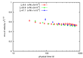
Figure 3: Evolution of the rms of velocity. Color and symbol are the same as in Figure 1.

In Figure 4 we plot the evolution of the differential energy spectrum of the axion radiation, $\frac{d(a^{4}\rho_{\rm rad})}{d\ln k}$, for $v/M_{*}=0.005$. This demonstrates two aspects of the axion radiation from the axion strings. One is that energy spectrum has a peak at low momenta and decays quickly towards higher ones. The other is that the spectral peaks moves towards lower momenta as time advances.

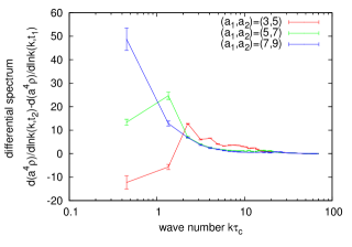
Figure 4: Differential spectrum between two scale factors ($a_{1}$, $a_{2}$) for the case of $v/M_{*}=0.005$.

To quantify the evolution of the spectral peaks, let us define

$$\epsilon(t)=\frac{t}{2\pi a\overline{k^{-1}}(t)},$$ (11)

where $\overline{k^{-1}}$ is the mean inverse momentum of radiated axion at $t$ defined as

$$\overline{k^{-1}}\equiv\frac{\frac{d}{dt}\int dkk^{-1}P_{\rm rad}(k,t)}{\frac{d}{dt}\int dkP_{\rm rad}(k,t)}$$ (12)

with $a^{-4}\int dkP_{\rm rad}$ being the energy density of the axion radiation. Roughly speaking, $\epsilon$ represents the mean wave number of radiated axion in units of the Hubble expansion rate.

Figure 5 shows the evolution of $\epsilon$. We confirm $\epsilon$ lies between two and four, which is largely consistent with [21, 27]. This supports the claim that radiated axions have typical momenta comparable to the Hubble expansion rate [13, 14, 16, 19, 20]. Due to the limitation of the number of bins, which is taken to 75 in our analysis, we cannot resolve the spectral peaks any longer when the mean wave number becomes comparable to the bin size. This is why we can trace $\epsilon$ only up to $t/d\sim 100$.

On the other hand, the wavelength of radiated axions are expected to be related to the correlation length of the strings, which is proportional to $1/\sqrt{\xi}$. This implies $\epsilon$ should be proportional to $\sqrt{\xi}$. Nonetheless, at this moment we cannot confirm such evolution of $\epsilon$ due to the lack of late-time measurements of $\epsilon$.

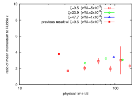
Figure 5: Evolution of the mean momentum of radiated axions in units of the Hubble expansion rate (see Eq. (11)). Color and symbol are the same as in Figure 1.

4 Discussion

Among the results we presented in the previous section, the growth of string parameter would have the most profound significance. While field theoretic simulation of physical strings cannot trace $t/d\gtrsim\mathcal{(}N_{g}^{1/3})$, $\log(t/d)$ can be as large as $70$ at the time of the QCD phase transition given $10^{9}\,{\rm GeV}\lesssim v\lesssim 10^{11}$ GeV, where the lower and upper bounds come from astrophysical consideration and cosmological axion abundance, respectively [32, 33, 10]. This means even the merely logarithmic growth can enhance $\xi$ by a factor of seven or larger .

The number of axions radiated from strings is proportional to the number of axion strings and inversely proportional to the typical momentum of radiated axions. The former is proportional to $\xi$. On the other hand, the latter is expected to be proportional to $\sqrt{\xi}$, though we couldn’t confirm this in our present simulation. Assuming that the axion momentum grows in proportion to $\sqrt{\xi}$, we expect the axion abundance is proportional $\sqrt{\xi}$. Our results indicates the abundance of axion can be enhanced by a factor of two or three. This should give a large impact not only on the constraints on the decay constant $f_{a}$ from overabundance of the axion CDM but also detection experiments, which target the mass of axion or $f_{a}\propto v$ with which the axion accounts for the observed CDM density.

Logarithmic growth in the string parameter is reported in [35, 36, 37]. However, the relation between our observation and theirs is not at all clear. This is because there is a crucial difference between the two simulations. Our strings are physical (i.e. constant string width), while the strings in [35, 36, 37] are so-called fat strings (i.e. string width growing in time). As discussed in [17], the radiation backreaction, which should be crucial in the dynamics of global strings [13, 38], is suppressed by the logarithm of $t/d$ (see also [30]). Since $d$ increases in fat strings, the extent of suppression of the radiation backreaction may deviate from that in physical strings. Therefore, results of fat strings cannot be easily identified with physical ones.

What is more puzzling is the nontrivial dependence of $\xi$ on the PQ breaking scale $v$. As seen in Figure 1, we found the magnitude of $\xi$ depends on $v$. Although previously reported values of $\xi$ have also been varying among literature [21, 30, 26, 27], the discrepancy has not been paid much attention due to statistical errors. Thanks to larger box size available at given $t$, the discrepancy in $\xi$ is manifested in our analysis with enough significance.

Such dependence apparently conflicts with the prediction of one-scale model [39, 40, 41]. Moreover, the dependence of $\xi$ on $v$ is not monotonic. As can be seen from Figure 1, the magnitude of $\xi$ fluctuates as $v/M_{*}$ is decreased from $0.005$ to $0.001$. This may indicate existence of competing effects, which explicitly depend on the PQ breaking scale.

At the moment, the physical origin of the logarithmic growth of the string parameter $\xi$ and its dependence on $v$ is still cloaked. As noted above, the efficiency of the energy loss of strings through radiation is suppressed by $\log(t/d)$. We speculate this can at least partially account for the logarithmic growth of $\xi$. Nonetheless, more rigorous investigation is required before we conclude this is the dominant cause. In view of the impact, scrutiny of the origin cannot be stressed too much. We pursue more detailed analysis with extensive parameter range and physical interpretation in the future publication [34].

We have also computed the spectrum of the axion radiated from the axion strings. The result is largely in agreement with the previous studies [21, 27]. We have confirmed the spectral peak stays around a few time larger than the Hubble expansion rate.

Note added: After we have finished writing the substantial part of the present manuscript we became aware of a paper by Gorghetto, Hardy, and Villadoro, who performed very similar numerical analysis [42].

References

- [1] S. Weinberg, Phys. Rev. Lett. 40, 223 (1978).
- [2] F. Wilczek, Phys. Rev. Lett. 40, 279 (1978).
- [3] R. D. Peccei and H. R. Quinn, Phys. Rev. Lett. 38, 1440 (1977).
- [4] M. Kawasaki and K. Nakayama, Ann. Rev. Nucl. Part. Sci. 63, 69 (2013) doi:10.1146/annurev-nucl-102212-170536 [arXiv:1301.1123 [hep-ph]].
- [5] D. J. E. Marsh, Phys. Rept. 643, 1 (2016) doi:10.1016/j.physrep.2016.06.005 [arXiv:1510.07633 [astro-ph.CO]].
- [6] P. Sikivie, Phys. Rev. Lett. 51, 1415 (1983) Erratum: [Phys. Rev. Lett. 52, 695 (1984)]. doi:10.1103/PhysRevLett.51.1415, 10.1103/PhysRevLett.52.695.2
- [7] R. Battesti et al., Lect. Notes Phys. 741, 199 (2008) doi:10.1007/978-3-540-73518-2_10 [arXiv:0705.0615 [hep-ex]].
- [8] P. W. Graham, I. G. Irastorza, S. K. Lamoreaux, A. Lindner and K. A. van Bibber, Ann. Rev. Nucl. Part. Sci. 65, 485 (2015) doi:10.1146/annurev-nucl-102014-022120 [arXiv:1602.00039 [hep-ex]].
- [9] I. G. Irastorza and J. Redondo, arXiv:1801.08127 [hep-ph].
- [10] A. Ringwald, L. Rosenberg, G. Rybka, “Axions and Other Similar Particles”, in The Review of Particle Physics (2018) M. Tanabashi et al. (Particle Data Group), Phys. Rev. D 98, 030001 (2018).
- [11] M. Kawasaki, K. Saikawa and T. Sekiguchi, Phys. Rev. D 91, no. 6, 065014 (2015) doi:10.1103/PhysRevD.91.065014 [arXiv:1412.0789 [hep-ph]].
- [12] T. Hiramatsu, M. Kawasaki, K. Saikawa and T. Sekiguchi, JCAP 1301, 001 (2013) doi:10.1088/1475-7516/2013/01/001 [arXiv:1207.3166 [hep-ph]].
- [13] R. L. Davis, Phys. Rev. D 32, 3172 (1985). doi:10.1103/PhysRevD.32.3172
- [14] R. L. Davis, Phys. Lett. B 180, 225 (1986). doi:10.1016/0370-2693(86)90300-X
- [15] D. Harari and P. Sikivie, Phys. Lett. B 195, 361 (1987). doi:10.1016/0370-2693(87)90032-3
- [16] R. L. Davis and E. P. S. Shellard, Nucl. Phys. B 324, 167 (1989). doi:10.1016/0550-3213(89)90187-9
- [17] A. Dabholkar and J. M. Quashnock, Nucl. Phys. B 333, 815 (1990). doi:10.1016/0550-3213(90)90140-9
- [18] C. Hagmann and P. Sikivie, Nucl. Phys. B 363, 247 (1991). doi:10.1016/0550-3213(91)90243-Q
- [19] R. A. Battye and E. P. S. Shellard, Nucl. Phys. B 423, 260 (1994) doi:10.1016/0550-3213(94)90573-8 [astro-ph/9311017].
- [20] R. A. Battye and E. P. S. Shellard, Phys. Rev. Lett. 73, 2954 (1994) Erratum: [Phys. Rev. Lett. 76, 2203 (1996)] doi:10.1103/PhysRevLett.73.2954, 10.1103/PhysRevLett.76.2203 [astro-ph/9403018].
- [21] M. Yamaguchi, M. Kawasaki and J. Yokoyama, Phys. Rev. Lett. 82, 4578 (1999) doi:10.1103/PhysRevLett.82.4578 [hep-ph/9811311].
- [22] M. Yamaguchi, Phys. Rev. D 60, 103511 (1999) doi:10.1103/PhysRevD.60.103511 [hep-ph/9907506].
- [23] M. Yamaguchi, J. Yokoyama and M. Kawasaki, Phys. Rev. D 61, 061301 (2000) doi:10.1103/PhysRevD.61.061301 [hep-ph/9910352].
- [24] C. Hagmann, S. Chang and P. Sikivie, Phys. Rev. D 63, 125018 (2001) doi:10.1103/PhysRevD.63.125018 [hep-ph/0012361].
- [25] M. Yamaguchi and J. Yokoyama, Phys. Rev. D 66, 121303 (2002) doi:10.1103/PhysRevD.66.121303 [hep-ph/0205308].
- [26] M. Yamaguchi and J. Yokoyama, Phys. Rev. D 67, 103514 (2003) doi:10.1103/PhysRevD.67.103514 [hep-ph/0210343].
- [27] T. Hiramatsu, M. Kawasaki, T. Sekiguchi, M. Yamaguchi and J. Yokoyama, Phys. Rev. D 83, 123531 (2011) doi:10.1103/PhysRevD.83.123531 [arXiv:1012.5502 [hep-ph]].
- [28] T. Hiramatsu, M. Kawasaki, K. Saikawa and T. Sekiguchi, Phys. Rev. D 85, 105020 (2012) Erratum: [Phys. Rev. D 86, 089902 (2012)] doi:10.1103/PhysRevD.86.089902, 10.1103/PhysRevD.85.105020 [arXiv:1202.5851 [hep-ph]].
- [29] D. P. Bennett and F. R. Bouchet, Phys. Rev. D 41, 2408 (1990). doi:10.1103/PhysRevD.41.2408
- [30] J. N. Moore, E. P. S. Shellard and C. J. A. P. Martins, Phys. Rev. D 65, 023503 (2002) doi:10.1103/PhysRevD.65.023503 [hep-ph/0107171].
- [31] M. Hindmarsh, S. Stuckey and N. Bevis, Phys. Rev. D 79 (2009) 123504 doi:10.1103/PhysRevD.79.123504 [arXiv:0812.1929 [hep-th]].
- [32] M. S. Turner, Phys. Rept. 197, 67 (1990).
- [33] G. G. Raffelt, Phys. Rept. 198, 1 (1990).
- [34] M. Kawasaki, T. Sekiguchi, M. Yamaguchi and J. Yokoyama, in prep.
- [35] L. Fleury and G. D. Moore, JCAP 1601, 004 (2016) doi:10.1088/1475-7516/2016/01/004 [arXiv:1509.00026 [hep-ph]].
- [36] V. B. Klaer and G. D. Moore, JCAP 1710, 043 (2017) doi:10.1088/1475-7516/2017/10/043 [arXiv:1707.05566 [hep-ph]].
- [37] V. B. .Klaer and G. D. .Moore, JCAP 1711, no. 11, 049 (2017) doi:10.1088/1475-7516/2017/11/049 [arXiv:1708.07521 [hep-ph]].
- [38] A. Vilenkin and E. P. S. Shellard, “Cosmic Strings and Other Topological Defects,” (Cambridge University Press, Cambridge, U.K., 1994).
- [39] T. W. B. Kibble, Nucl. Phys. B 252, 227 (1985) Erratum: [Nucl. Phys. B 261, 750 (1985)]. doi:10.1016/0550-3213(85)90439-0, 10.1016/0550-3213(85)90596-6
- [40] D. P. Bennett, Phys. Rev. D 33, 872 (1986) Erratum: [Phys. Rev. D 34, 3932 (1986)]. doi:10.1103/PhysRevD.34.3932.2, 10.1103/PhysRevD.33.872
- [41] C. J. A. P. Martins and E. P. S. Shellard, Phys. Rev. D 65, 043514 (2002) doi:10.1103/PhysRevD.65.043514 [hep-ph/0003298].
- [42] M. Gorghetto, E. Hardy and G. Villadoro, arXiv:1806.04677 [hep-ph].