Phase estimation for an SU(1,1) interferometer in the presence of phase diffusion and photon losses

Abstract

We theoretically study the quantum Fisher information (QFI) of the SU(1,1) interferometer with phase shifts in two arms taking account of realistic noise effects. A generalized phase transform including the phase diffusion effect is presented by the purification process. Based on this transform, the analytical QFI and the bound to the quantum precision are derived when considering the effects of phase diffusion and photon losses simultaneously. To beat the standard quantum limit with the reduced precision of phase estimation due to noisy, the upper bounds of decoherence coefficients as a function of total mean photon number are given.

I Introduction

The estimation of the optical phase has been proposed and demonstrated using different quantum strategies and interferometric setups Helstrom67 ; Holevo82 ; Caves81 ; Braunstein94 ; Braunstein96 ; Lee02 ; Giovannetti06 ; Zwierz10 ; Giovannetti04 ; Giovannetti11 ; Toth ; Degen . In particular, interferometers can provide the most precise measurements, for example, the gravitational waves can be observed by the advanced Laser Interferometer Gravitational-Wave Observatory (LIGO) Abbott . The Mach-Zehnder interferometer (MZI) and its variants have been used as a generic model to realize precise measurement of phase. In 1986, an SU(1,1) interferometer was introduced by Yurke et al. Yurke86 , where two nonlinear beam splitters (NBSs) take the place of two linear beam splitters (BSs) in the traditional MZI. It is called the SU(1,1) interferometer because it is described by the SU(1,1) group, as opposed to the SU(2) one for BSs. The phase sensitivity of an SU(1,1) interferometer scales as $1/n$ instead of $1/\sqrt{n}$, where $n$ is the average number of photons inside the interferometer. This enhanced sensitivity has attracted the attention of many researchers to study this interferometer, which have been constructed with several platforms, such as light Plick ; Jing11 ; Hudelist ; Du18 , atoms Gross ; Peise ; Gabbrielli ; Linnemann16 , nonlinear crystals Lemieux16 ; Manceau17 , and matter-light hybrid ChenPRL15 ; Yama ; Haine ; Szigeti ; Haine16 ; Yuan16 ; Barzanjeh . Recently, a simplified variation of the SU(1,1) interferometer-truncated SU(1,1) interferometer has been presented, which can achieve the same phase sensitivity Anderson1 ; Anderson2 ; Gupta .

For an SU(1,1) interferometer, several measurement methods, such as intensity detection Ou ; Marino , homodyne detection Ou ; Li14 and parity detection Li16 , have been studied to analyze phase estimation. Every measurement method has its own superiority and these several detection methods were compared Li16 ; Li18 . In general, it is difficult to optimize over the detection methods to obtain the optimal estimation protocols. Fortunately, the quantum Fisher information (QFI) is the intrinsic information in the quantum state and is not related to the actual measurement procedure Braunstein94 ; Braunstein96 . It characterizes the maximum amount of information that can be extracted from quantum experiments about an unknown parameter using the best (and ideal) measurement device. It establishes the best precision that can be attained with a given quantum probe. We have investigated the QFIs of the SU(1,1) interferometer with several different input states for lossless case Li16 ; Gong17c .

Because there are inevitable interactions with the surrounding environment, in the presence of environment noise, the QFI and the corresponding measurement precision will be reduced, which have been studied by many researchers Dem09 ; Dem12 ; Escher12 ; Berry13 ; Chaves ; Dur ; Kessler ; Brivio ; Alipour ; Escher11 ; Genoni11 ; Genoni12 ; Sparaciari ; Feng . For interferometers, there are three typical decoherence processes that should be taken into account: (1) photon losses, which may happen at any stage of the phase process and is modeled by the fictitious BS introduced in the interferometer arms. The effect of photon losses on the interferometry has been studied Dem09 ; Dem12 ; Escher11 , where this decoherence process can be described by a set of Kraus operators. (2) phase diffusion, which represents the effect of fluctuation of the estimated phase delay. Recently, Escher et al. Escher12 presented a variational approach to show an analytical bound based on purification techniques, which has an explicit dependence on the mathematical description of the noise. In some physical processes, such as path length fluctuations of a stabilized interferometer, thermal fluctuations of an optical fibre, phase and phase diffusion may vary in time Trapani . The weak measurements and joint estimation were used to deal the phase and phase diffusion simultaneously for quantum metrology Vidrighin ; Altorio . Recently, using this variational approach, Zwierz and Wiseman extended the phase diffusion noise from linear to nonlinear and gave the precision bound for a second-order phase-diffusion noise Zwierz14 . (3) detection losses Ou ; Sparaciari . The influence of the detection loss on the phase sensitivity is less than the photon loss inside the interferometer. As for SU(1,1) interferometers, the influence of detection loss can be suppressed by using unbalanced gains in the two nonlinear processes Manceau17 ; Giese .

In addition to the detection losses, the photon losses and phase diffusion need to be investigated. Although, the photon losses effect on phase estimation in an SU(1,1) interferometer have been studied Ou ; Marino ; Gong17 . However, a more accurate and efficient scheme is required to estimate the phase shift considering the effects of phase diffusion and photon losses simultaneously. In this paper, we derive the QFI of the SU(1,1) interferometer in the presence of phase diffusion and photon losses simultaneously based on the generalized phase transform. Then the phase estimation precision as a function of the decoherence coefficients is discussed and the upper bound of decoherence coefficients to beat the standard quantum limit is given.

Our article is organized as follows. In Sec. II, we briefly describe the generalized decoherence model. In Sec. III, the form of generalized phase transform is given based on the purification process, based on which the Kraus operators including the photon losses and phase diffusion coefficients are derived. In Sec. IV, the QFI of the SU(1,1) interferometer in the presence of losses and phase diffusion simultaneously is obtained and discussed. Finally, we conclude with a summary of our results.

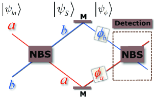
Figure 1: Schematic diagram of an SU(1,1) interferometer. $|\psi_{in}\rangle$, $|\psi_{S}\rangle$ and $|\psi_{\phi}\rangle$ are the different states of the evolution process without decoherence. $\phi_{a}$ and $\phi_{b}$ are the phase shifts arms $a$ and $b$, respectively.

II Decoherence model of SU(1,1) interferometers

Decoherence is a consequence of the uncontrolled interactions of a quantum system with the environment. Effects of decoherence inside an interferometer should be taken into account. Recently, Escher et al. Escher11 developed a general formalism in the presence of losses. Here, we extend this model to derive the QFI in the presence of losses and phase diffusion simultaneously.

Given an initial pure state $\hat{\rho}_{0S}=|\psi_{S}\rangle\langle\psi_{S}|$ of a system $S$, in the presence of losses and phase diffusion the evolution of system is non-unitary. However, in a bigger space the final enlarged state is given by

$$\hat{\rho}_{S,E,E^{\prime}}=\hat{U}_{S,E,E^{\prime}}(\eta,\beta,\phi)\hat{\rho}_{0S}\otimes\hat{\rho}_{0E}\otimes\hat{\rho}_{0E^{\prime}}\hat{U}_{S,E,E^{\prime}}^{{\dagger}},$$ (1)

where $\hat{U}_{S,E,E^{\prime}}(\eta,\beta,\phi)$ is the corresponding unitary operator of the enlarged state ($S+E+E^{\prime}$). $\hat{\rho}_{0E}=|0_{E}\rangle\langle 0_{E}|$, $|0_{E}\rangle$ is the initial state of the phase diffusion model, and $\beta$ is the phase diffusion coefficient ($\beta=0$, corresponding to no diffusion; $\beta=\infty$, corresponding to maximum diffusion). $\hat{\rho}_{0E^{\prime}}=|0_{E^{\prime}}\rangle\langle 0_{E^{\prime}}|$, $|0_{E^{\prime}}\rangle$ is the initial state of the photon loss environment. $\eta$ quantifies the photon losses (from $\eta=1$, lossless case, to $\eta=0$, complete absorption).

When the environment $E^{\prime}$ is not monitored, one may take the partial trace with respect to $E^{\prime}$,

$$\hat{\rho}_{S,E} =\mathrm{Tr}_{E^{\prime}}\{\hat{U}_{S,E,E^{\prime}}(\eta,\beta,\phi)[\hat{\rho}_{0S}\otimes\hat{\rho}_{0E}\otimes\hat{\rho}_{0E^{\prime}}]\hat{U}_{S,E,E^{\prime}}^{{\dagger}}\}$$

$$=\sum_{l}\langle l_{E^{\prime}}|\hat{U}_{S,E,E^{\prime}}(\eta,\beta,\phi)[\hat{\rho}_{0S}\hat{\rho}_{0E}\hat{\rho}_{0E^{\prime}}]\hat{U}_{S,E,E^{\prime}}^{{\dagger}}|l_{E^{\prime}}\rangle$$

$$=\sum_{l}\hat{\Pi}_{l}(\eta,\beta,\phi)\hat{\rho}_{0S}\hat{\rho}_{0E}\hat{\Pi}_{l}^{{\dagger}}(\eta,\beta,\phi),$$ (2)

where $|l_{E^{\prime}}\rangle$ are the orthogonal states of the environment $E^{\prime}$, and $\hat{\Pi}_{l}(\eta,\beta,\phi)=\langle l_{E^{\prime}}|\hat{U}_{S,E,E^{\prime}}(\eta,\beta,\phi)|0_{E^{\prime}}\rangle$ are Kraus operators which not only describe the photon losses process, but also include the phase evolution. Without considering photon losses and only considering the phase diffusion, based on the purified process the enlarged system-environment ($S+E$) state is written as

$$\left|\Phi_{S,E}(\phi)\right\rangle=\tilde{U}(\phi,\beta)\left|\psi_{S}\right\rangle\left|0_{E}\right\rangle,$$ (3)

where $\tilde{U}(\phi,\beta)$ is the generalized phase transformation including the phase diffusion coefficient $\beta$ compared to the phase transform $\hat{U}(\phi)$ of the ideal interferometer. Usually, $\hat{\Pi}_{l}(\eta,\phi,\beta)$ may be written as $\hat{\Lambda}_{l}(\eta)\tilde{U}(\phi,\beta)$ or $\tilde{U}(\phi,\beta)\hat{\Lambda}_{l}(\eta)$ where $\hat{\Lambda}_{l}(\eta)$ are Kraus operators without considering the phase shift. In realistic systems the photon losses are distributed throughout the arms of interferometer, not an event concentrated either before or after the phase $\tilde{U}(\phi,\beta)$ is displaced. Then $\hat{\Lambda}_{l}(\eta)\tilde{U}(\phi,\beta)$ or $\tilde{U}(\phi,\beta)\hat{\Lambda}_{l}(\eta)$ are just a matter of convenience. An optimized Kraus operator $\hat{\Pi}_{l}(\eta,\beta,\phi)$ can be obtained by making the QFI is minimal, which will be given in the next section.

For the enlarged system-environment ($S+E+E^{\prime}$) state $|\Psi_{SEE^{\prime}}\rangle=\hat{U}_{SEE^{\prime}}(\eta,\beta,\phi)|\psi_{S}\rangle|0_{E^{\prime}}\rangle|0_{E}\rangle$, the QFI $\mathcal{C}_{Q}$ is given by PezzBook

$$\mathcal{C}_{Q} =4\langle\Delta\hat{H}_{S,E,E^{\prime}}^{2}\rangle=4[\langle 0_{E^{\prime}}|\langle 0_{E}|\langle\psi_{S}|\hat{H}_{S,E,E^{\prime}}^{2}|\psi_{S}\rangle|0_{E}\rangle|0_{E^{\prime}}\rangle$$

$$-\langle 0_{E^{\prime}}|\langle 0_{E}|\langle\psi_{S}|\hat{H}_{S,E,E^{\prime}}|\psi_{S}\rangle|0_{E}\rangle|0_{E^{\prime}}\rangle^{2}],$$ (4)

where $\hat{H}_{S,E,E^{\prime}}=i(d\hat{U}_{S,E,E^{\prime}}^{{\dagger}}(\eta,\beta,\phi)/d\phi)\hat{U}_{S,E,E^{\prime}}(\eta,\beta,\phi)$. The expression $\langle\Delta\hat{H}_{S,E,E^{\prime}}^{2}\rangle$ may be rewritten as

$$\langle\Delta\hat{H}_{S,E,E^{\prime}}^{2}\rangle =\left(\frac{d\langle\Psi_{SEE^{\prime}}|}{dx}\right)\left(\frac{d|\Psi_{SEE^{\prime}}\rangle}{dx}\right)$$

$$-\left|\left(\frac{d\langle\Psi_{SEE^{\prime}}|}{dx}\right)|\Psi_{SEE^{\prime}}\rangle\right|^{2}.$$ (5)

Therefore, in terms of the initial state of the system $|\psi_{S}\rangle$, the initial state of the phase diffusion model $|0_{E}\rangle$, and the Kraus operators $\hat{\Pi}_{l}(\eta,\beta,\phi)$, the enlarged state can be written as $|\Psi_{SEE^{\prime}}\rangle=\sum_{l}\hat{\Pi}_{l}(\eta,\beta,\phi)|\psi\rangle_{S}\left|0_{E}\right\rangle|l_{E^{\prime}}\rangle$, then the value of $\mathcal{C}_{Q}$ is given by Escher11

$$\mathcal{C}_{Q} =4\langle\Delta\hat{H}_{S,E,E^{\prime}}^{2}\rangle=4[\langle 0_{E}|\langle\psi_{S}|\hat{H}_{1}|\psi_{S}\rangle|0_{E}\rangle$$

$$-\left|\langle 0_{E}|\langle\psi_{S}|\hat{H}_{2}|\psi_{S}\rangle|0_{E}\rangle\right|^{2}],$$ (6)

where

$$\hat{H}_{1} =\sum_{l}\frac{d\hat{\Pi}_{l}^{{\dagger}}(\eta,\beta,\phi)}{d\phi}\frac{d\hat{\Pi}_{l}(\eta,\beta,\phi)}{d\phi},\text{\ }$$

$$\hat{H}_{2} =i\sum_{l}\frac{d\hat{\Pi}_{l}^{{\dagger}}(\eta,\beta,\phi)}{d\phi}\hat{\Pi}_{l}(\eta,\beta,\phi).$$ (7)

Because the additional freedom supplied by the environment ($E+E^{\prime}$) should increase the QFI. Therefore, the QFI $\mathcal{F}_{Q}$ only describing the system should be smaller or equal to the $\mathcal{C}_{Q}$ obtained on the system plus environment ($E+E^{\prime}$). It is possible to determine the value of QFI $\mathcal{F}_{Q}[\hat{\rho}_{S}]$ by two steps minimizing the upper bound $\mathcal{C}_{Q}[\hat{\rho}_{S,E,E^{\prime}}]$. One is by optimizing over all possible measurements $\hat{\Pi}_{l}$, the other is by the minimum all possible purifications $\left|\Phi_{S,E}(\phi)\right\rangle$. The relation between $\mathcal{F}_{Q}[\hat{\rho}_{S}]$ and $\mathcal{C}_{Q}[\hat{\rho}_{S,E,E^{\prime}}]$ is written as

$$\mathcal{F}_{Q}=\underset{\{\hat{\Pi}_{l}(\eta,\beta,\phi),\text{ }\left|\Phi_{S,E}(\phi)\right\rangle\}}{\min}\mathcal{C}_{Q}\left[\hat{\rho}_{0S}\hat{\rho}_{0E},\hat{\Pi}_{l}(\eta,\beta,\phi)\right].$$ (8)

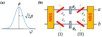
Figure 2: Lossy interferometer model. (a) The phase diffusion corresponds to the application of a random, Gaussian-distributed phase shift $\varphi$ with variance $2\beta^{2}$ and the mean equal to the estimated parameter $\phi$. (b) The losses in the interferometer are modeled by adding fictitious beam splitters (I) before and (II) after the phase shifts $\phi_{1}$ and $\phi_{2}$. $\hat{v}_{a}$ and $\hat{v}_{b}$ represent the vacuum.

Next, we will describe the unitary phase transform $U(\phi)$, the generalized phase transform $\tilde{U}(\phi,\beta)$, and the optimized Kraus operators $\hat{\Pi}_{l}(\eta,\beta,\phi)$ including phase diffusion coefficients and photon loss coefficients.

II.1 Phase transformation $\hat{U}(\phi)$

An SU(1,1) interferometer is shown in Fig. 1, and the annihilation operators of the two modes $a$, $b$ are denoted as $\hat{a}$, $\hat{b}$, respectively. After the first NBS, the two beams sustain phase shifts, i.e., mode $a$ undergoes a phase shift of $\phi_{a}$ and mode $b$ undergoes a phase shift of $\phi_{b}$. In an ideal interferometer, the transformation of the incoming state vector $\left|\psi_{S}\right\rangle$ in the Schrödinger picture is given as following

$$|\psi_{\phi}\rangle=\hat{U}(\phi)\left|\psi_{S}\right\rangle,$$ (9)

and

$$\hat{U}(\phi) =\exp\left(i\phi_{a}\hat{n}_{a}\right)\exp(i\phi_{b}\hat{n}_{b})$$

$$=\exp(i\phi\hat{K}_{z})\exp[i(\phi_{a}-\phi_{b})\hat{J}_{z}-i\phi/2],$$ (10)

where $\phi=\phi_{a}+\phi_{b}$, $\hat{K}_{z}=(\hat{n}_{a}+\hat{n}_{b}+1)/2$, $\hat{J}_{z}=(\hat{n}_{a}-\hat{n}_{b})/2$, $\hat{n}_{a}=\hat{a}^{\dagger}\hat{a}$, and $\hat{n}_{b}=\hat{b}^{\dagger}\hat{b}$. The operator $e^{i(\phi_{a}-\phi_{b})\hat{J}_{z}}$ gives rise to phase factors which do not contribute to the expectation values of number operators.

II.2 Generalized phase transformation $\tilde{U}(\phi,\beta)$

In an SU(1,1) interferometer, it is vital to take into account the unavoidable influence of noise on the ultimate precision limits. The collective dephasing or the phase noise represents the effect of fluctuation of the estimated phase shift $\phi$, which is also termed as phase diffusion. Now, we derive the generalized $\tilde{U}(\phi,\beta)$ including the phase diffusion.

In the Markovian limit, the phase diffusion environment is static, and the diffusion coefficient is a time-independent variance. When the noisy environments cannot be described in terms of a Markovian master equation, the time-dependent variance and the dynamical properties of the environment should be considered Trapani . The phase diffusion of state can be modeled by the effects of the radiation pressure on the interferometer mirror, where the light is being reflected from a mirror which position fluctuations are randomly changing the effective optical length Escher11 . Assuming the measuring time is much less than the vibration period of the mirror, the evolution between the light field and the mirror is taken as

$$\exp[i(\sqrt{2}\beta)\hat{n}(\hat{b}_{E}+\hat{b}_{E}^{{\dagger}})]=\exp[i2\beta\hat{n}\hat{x}_{E}],$$ (11)

where $\hat{n}$ is the number operator of light field, $\hat{x}_{E}$ ($=(\hat{b}_{E}+\hat{b}_{E}^{{\dagger}})/\sqrt{2}$) and $\hat{b}_{E}$ are the position and annihilate operators of mirror. Assuming the mirrors as the environments in the ground state of a quantum oscillator $\left|0_{E_{a}}\right\rangle$ and $\left|0_{E_{b}}\right\rangle$ before interaction with the light beam, the final state of the combined system ($S+E$) of the probe and the mirror is given by

$$\left|\Phi_{S,E}(\phi)\right\rangle =\hat{U}_{S,E}(\phi,\beta_{a},\beta_{b})|\psi_{S}\rangle|0_{E}\rangle=e^{i\phi_{a}\hat{n}_{a}}e^{i\phi_{b}\hat{n}_{b}}$$

$$\times e^{i(2\beta_{a})\hat{n}_{a}\hat{x}_{E_{a}}}e^{i(2\beta_{b})\hat{n}_{b}\hat{x}_{E_{b}}}\left|\psi_{S}\right\rangle\left|0_{E_{a}}\right\rangle\left|0_{E_{b}}\right\rangle$$

$$=e^{i\phi(\hat{K}_{z}-\frac{1}{2})}e^{i(\phi_{a}-\phi_{b})\hat{J}_{z}}e^{i(2\beta_{a})\hat{n}_{a}\hat{x}_{E_{a}}}$$

$$\times e^{i(2\beta_{b})\hat{n}_{b}\hat{x}_{E_{b}}}\left|\psi_{S}\right\rangle\left|0_{E_{a}}\right\rangle\left|0_{E_{b}}\right\rangle,$$ (12)

where $\hat{U}_{S,E}(\phi,\beta_{a},\beta_{b})$ is the corresponding unitary operator acting on the enlarged state. $\beta_{a}$ and $\beta_{b}$ are diffusion coefficients in arms $a$ and $b$, respectively. This particular purification also leads to a trivial noiseless upper bound on the QFI as in Ref Escher12 . However, the purified unitary evolution is integrally written as

$$|\Psi_{S,E}\rangle=\hat{u}_{E}(x)|\Phi_{S,E}\rangle=\hat{u}_{E}(x)\hat{U}_{S,E}(x)\left|\psi_{S}\right\rangle\left|0_{E_{a}}\right\rangle\left|0_{E_{b}}\right\rangle,$$ (13)

where $\hat{u}_{E}$ is a unitary operator acting only on the $E$. To the same evolution of system $S$, many evolution of systems of $S+E$ lead to possibly different values of the QFI. Therefore, a stronger upper bound can be obtained by minimizing $\mathcal{C}_{Q}[|\Psi_{S,E}\rangle]$ over all purifications of the system $S$. Inserting the evolution operator $\hat{u}_{E}(x)\hat{U}_{S,E}(x)$ into Eq. (4) without considering the enviroment $E^{\prime}$, we obtain $\hat{H}_{S,E}$ and the corresponding QFI $\mathcal{C}_{Q}=4\langle\Delta\hat{H}_{S,E}^{2}\rangle$. As $\langle\Delta\hat{H}_{S,E}^{2}\rangle$ only depends on $\hat{u}_{E}(x)$ through $\hat{h}_{E}(x)$, which is defined as $\hat{h}_{E}(x)=i(d\hat{u}_{E}^{{\dagger}}/dx)\hat{u}_{E}$ Escher12 .

Next, we follow the method of Escher et al. Escher12 to derive an optimal $\hat{h}_{E}^{(\mathrm{opt})}$, from which we can obtain a tighter upper bound to the QFI of the system $S$, and then the corresponding generalized phase transform $\tilde{U}(\phi,\beta)$. The optimal Hermitian operator $\hat{h}_{E}^{(\mathrm{opt})}$ is given by

$$\frac{1}{2}\left(\hat{h}_{E}^{(\mathrm{opt})}\hat{\rho}_{E}+\hat{\rho}_{E}\hat{h}_{E}^{(\mathrm{opt})}\right)=\mathrm{Tr}_{S}\{D\left[\hat{\rho}_{S,E}\right]\},$$ (14)

where $\hat{\rho}_{E}=\mathrm{Tr}_{S}[\left|\Phi_{S,E}\right\rangle\left\langle\Phi_{S,E}\right|]=\mathrm{Tr}_{S}[\hat{\rho}_{S,E}]$ is the reduced density matrix in the $E$ space, and $D\left[\hat{\rho}_{S,E}\right]$ is defined as

$$D\left[\hat{\rho}_{S,E}\right]\equiv\frac{i}{2}\left[\frac{d\left|\Phi_{S,E}\right\rangle}{dx}\left\langle\Phi_{S,E}\right|-\left|\Phi_{S,E}\right\rangle\frac{d\left\langle\Phi_{S,E}\right|}{dx}\right].$$ (15)

From Eq. (12), the reduced density matrix of the mirror associated with the purification $\left|\Phi_{S,E}(\phi)\right\rangle$ is

$$\hat{\rho}_{E} =\sum_{n_{a}}\sum_{n_{b}}\left|\rho_{n_{a}n_{b}}\right|^{2}\left|i\sqrt{2}\beta_{a}n_{a}\right\rangle_{E_{a}}\left\langle i\sqrt{2}\beta_{a}n_{a}\right|$$

$$\times\left|i\sqrt{2}\beta_{b}n_{b}\right\rangle_{E_{b}}\left\langle i\sqrt{2}\beta_{b}n_{b}\right|,$$ (16)

and

$$\mathrm{Tr}_{S}\{D\left[\hat{\rho}_{S,E}\right]\} =-\frac{1}{2}\sum_{n_{a}}\sum_{n_{b}}[(\frac{-i\hat{b}_{E_{a}}}{2\sqrt{2}\beta_{a}}+\frac{-i\hat{b}_{E_{b}}}{2\sqrt{2}\beta_{b}})\hat{\rho}_{E}$$

$$+\hat{\rho}_{E}(\frac{i\hat{b}_{E_{a}}^{{\dagger}}}{2\sqrt{2}\beta_{a}}+\frac{i\hat{b}_{E_{b}}^{{\dagger}}}{2\sqrt{2}\beta_{b}})],$$ (17)

where $\hat{b}_{E_{i}}=(\hat{x}_{E_{i}}+i\hat{p}_{E_{i}})/\sqrt{2}$ with $\hat{p}_{E_{i}}$ being the dimensionless momentum operator of mirror ($i=a,b$). Therefore, the Eq. (14) can be rewritten as

$$\frac{1}{2}\left(\hat{h}_{E}^{(\mathrm{opt})}\hat{\rho}_{E}+\hat{\rho}_{E}\hat{h}_{E}^{(\mathrm{opt})}\right)=-\frac{1}{2}\sum_{n_{a}}\sum_{n_{b}}[(\frac{\hat{p}_{E_{a}}}{4\beta_{a}}+\frac{\hat{p}_{E_{b}}}{4\beta_{b}})\hat{\rho}_{E}$$

$$+\hat{\rho}_{E}(\frac{\hat{p}_{E_{a}}}{4\beta_{a}}+\frac{\hat{p}_{E_{b}}}{4\beta_{b}})-i(\frac{\hat{x}_{E_{a}}}{4\beta_{a}}+\frac{\hat{x}_{E_{b}}}{4\beta_{b}})\hat{\rho}_{E}$$

$$+i\hat{\rho}_{E}(\frac{\hat{x}_{E_{a}}}{4\beta_{a}}+\frac{\hat{x}_{E_{b}}}{4\beta_{b}})].$$ (18)

To get a tighter upper bound to the QFI of the system $S$, according to the Eq. (18) we can guess $\hat{h}_{E}^{(\mathrm{opt})}=\lambda(\hat{p}_{E_{a}}/4\beta_{a}+\hat{p}_{E_{b}}/4\beta_{b})$, and we can also obtain the optimal $\hat{u}_{E}(x)=\exp[i\phi\lambda(\hat{p}_{E_{a}}/4\beta_{a}+\hat{p}_{E_{b}}/4\beta_{b})]$ with $\lambda$ being a variational parameter Escher11 . The new purification process produces the following enlarged system-environment ($S+E$) state:

$$\left|\Phi_{S,E}(\phi)\right\rangle=\tilde{U}(\phi,\beta_{a},\beta_{b})\left|\psi_{S}\right\rangle\left|0_{E_{a}}\right\rangle\left|0_{E_{b}}\right\rangle,$$ (19)

where the generalized phase transform $\tilde{U}(\phi,\beta_{a},\beta_{b})$ is given by

$$\tilde{U}(\phi,\beta_{a},\beta_{b}) =e^{i\phi[\lambda(\hat{p}_{E_{a}}/4\beta_{a}+\hat{p}_{E_{b}}/4\beta_{b})+\hat{K}_{z}-\frac{1}{2}]}e^{i(\phi_{a}-\phi_{b})\hat{J}_{z}}$$

$$\times e^{i(2\beta_{a})\hat{n}_{a}\hat{x}_{E_{a}}}e^{i(2\beta_{b})\hat{n}_{b}\hat{x}_{E_{b}}}.$$ (20)

II.3 Kraus operators with noisy

Here, we derive the Kraus operators $\hat{\Pi}_{l}(\eta,\beta,\phi)$ including phase diffusion coefficients and photon loss coefficients based on the generalized phase transform $\tilde{U}(\phi,\beta_{a},\beta_{b})$.

As shown in Fig. 2(b), beam splitters are used as a model for the photon-loss mechanism Dem09 . After the photon passing through the virtual beam splitter, the evolution of the state can be described by a Kraus operator $\hat{\Lambda}_{l_{a}l_{b}}(\eta_{a},\eta_{b})=\sqrt{\frac{(1-\eta_{a})^{l_{a}}(1-\eta_{b})^{l_{b}}}{l_{a}!l_{b}!}}\eta_{a}^{\hat{n}_{a}/2}\eta_{b}^{\hat{n}_{b}/2}\hat{a}^{l_{a}}\hat{b}^{l_{b}}$, where $\eta_{i}$ quantifies the photon losses of arm $i$ ($\eta_{i}=1$, lossless case, $\eta_{i}=0$, complete absorption, $i=a,b$). Corresponding to the photon losses before or after the phase shifts, the Kraus operators including the generalized phase factor $\tilde{U}(\phi,\beta_{a},\beta_{b})$ are written as

$$\hat{\Pi}_{l_{a}l_{b}}(\eta_{a},\eta_{b},\beta_{a},\beta_{b},\phi) =\sqrt{\frac{(1-\eta_{a})^{l_{a}}(1-\eta_{b})^{l_{b}}}{l_{a}!l_{b}!}}$$

$$\times\tilde{U}(\phi,\beta_{a},\beta_{b})\eta_{a}^{\frac{\hat{n}_{a}}{2}}\eta_{b}^{\frac{\hat{n}_{b}}{2}}\hat{a}^{l_{a}}\hat{b}^{l_{b}},$$ (21)

or

$$\hat{\Pi}_{l_{a}l_{b}}(\eta_{a},\eta_{b},\beta_{a},\beta_{b},\phi) =\sqrt{\frac{(1-\eta_{a})^{l_{a}}(1-\eta_{b})^{l_{b}}}{l_{a}!l_{b}!}}$$

$$\times\eta_{a}^{\frac{\hat{n}_{a}}{2}}\eta_{b}^{\frac{\hat{n}_{b}}{2}}\hat{a}^{l_{a}}\hat{b}^{l_{b}}\tilde{U}(\phi,\beta_{a},\beta_{b}).$$ (22)

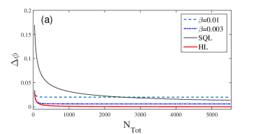
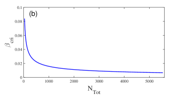
Figure 3: (a) The phase sensitivity $\Delta\phi$ versus $N_{\mathrm{Tot}}$ with $\beta=0.01$ (dashed line) and $\beta=0.003$ (dotted-dashed line), $g=2$. (b) The critical $\beta_{\mathrm{cri}}$ as a function of the total mean photon number inside the interferometer $N_{\mathrm{Tot}}$ where $g=2$, and $\beta_{a}$=$\beta_{b}$. Given a $N_{\mathrm{Tot}}$, the phase sensitivity $\Delta\phi$ beat the SQL when $\beta<\beta_{\mathrm{cri}}$.

By introducing two parameters $\gamma_{a}$ and $\gamma_{b}$, we define a family of Kraus operators, which can be used to minimize the value of $\mathcal{C}_{Q}$. Then a possible set of Kraus operators describing the phase diffusion and photon losses is given by

$$\hat{\Pi}_{l_{a}l_{b}}(\eta_{a},\eta_{b},\beta_{a},\beta_{b},\phi)=\sqrt{\frac{(1-\eta_{a})^{l_{a}}(1-\eta_{b})^{l_{b}}}{l_{a}!l_{b}!}}$$

$$\times e^{i(\phi_{1}-\phi_{2})(\hat{J}_{z}-\frac{\gamma_{a}l_{a}}{2}+\frac{\gamma_{b}l_{b}}{2})}$$

$$\times e^{i\phi[(\frac{\hat{n}_{a}-\gamma_{a}l_{a}}{2}+\lambda\frac{\hat{p}_{E_{a}}}{4\beta a})+(\frac{\hat{n}_{b}-\gamma_{b}l_{b}}{2}+\lambda\frac{\hat{p}_{E_{b}}}{4\beta_{b}})]}$$

$$\times e^{i[(\beta_{a}\hat{x}_{E_{a}}-\beta_{b}\hat{x}_{E_{b}})(\hat{n}_{a}-\gamma_{a}l_{a}-\hat{n}_{b}+\gamma_{b}l_{b})]}$$

$$\times e^{i[(\beta_{a}\hat{x}_{E_{a}}+\beta_{b}\hat{x}_{E_{b}})(\hat{n}_{a}-\gamma_{a}l_{a}+\hat{n}_{b}-\gamma_{b}l_{b})]}\eta_{a}^{\frac{\hat{n}_{a}}{2}}\eta_{b}^{\frac{\hat{n}_{b}}{2}}\hat{a}^{l_{a}}\hat{b}^{l_{b}},$$ (23)

where $\gamma_{i}$ describes the photon loss before ($\gamma_{i}=0$) and after ($\gamma_{i}=-1$) the phase shifts of arm $i$ ($i=a,b$).

III QFI of SU(1,1) interferometers

In this section, we use the above Kraus operators to obtain the QFI in the presence of photon losses and phase diffusion simultaneously.

Without decoherence, the definition of QFI for pure states is simplified to PezzBook

$$\mathcal{F}_{Q}=4(\left\langle\psi_{\phi}^{\prime}\right|\psi_{\phi}^{\prime}\rangle-\left|\left\langle\psi_{\phi}^{\prime}\right|\psi_{\phi}\rangle\right|^{2}),\text{ }\left|\psi_{\phi}^{\prime}\right\rangle=\frac{d\left|\psi_{\phi}\right\rangle}{d\phi}.$$ (24)

The QFI of an SU(1,1) interferometer can be worked out $\mathcal{F}_{Q}=4\langle\Delta^{2}\hat{K}_{z}\rangle$, where $\langle\Delta^{2}\hat{K}_{z}\rangle=\left\langle\psi_{S}\right|\hat{K}_{z}^{2}|\psi_{S}\rangle-\left|\left\langle\psi_{S}\right|\hat{K}_{z}|\psi_{S}\rangle\right|^{2}$. Further simplification, the QFI $\mathcal{F}_{Q}$ can be written as Gong17

$$\mathcal{F}_{Q}=\left\langle\Delta^{2}\hat{n}_{a}\right\rangle+\left\langle\Delta^{2}\hat{n}_{b}\right\rangle+2Cov[\hat{n}_{a},\hat{n}_{b}],$$ (25)

where $\left\langle\Delta^{2}\hat{n}_{i}\right\rangle=\langle\hat{n}_{i}^{2}\rangle-\langle\hat{n}_{i}\rangle^{2}$ $(i=a,b)$, and $Cov[\hat{n}_{a},\hat{n}_{b}]=\langle\hat{n}_{a}\hat{n}_{b}\rangle-\langle\hat{n}_{a}\rangle\langle\hat{n}_{b}\rangle$. $\langle\cdot\rangle$ and $\langle\Delta^{2}\cdot\rangle$ are the respective average and the variance calculated in the state $\left|\psi_{S}\right\rangle$.

In the presence of photon losses and phase diffusion simultaneously, the QFI can be obtained from the extend method of Eq. (6). With Eq. (23), the Hermitian operators $\hat{H}_{1,2}$ become

$$\hat{H}_{1} =\sum_{l_{a}=0}^{n_{a}}\sum_{l_{b}=0}^{n_{b}}\frac{d\hat{\Pi}_{l_{a}l_{b}}^{\dagger}}{d\phi}\frac{d\hat{\Pi}_{l_{a}l_{b}}}{d\phi}=\frac{1}{4}[(1+\lambda)$$

$$\times(\hat{n}_{a}+\hat{n}_{b}-\gamma_{a}^{\prime}\hat{S}_{a}-\gamma_{b}^{\prime}\hat{S}_{b})+2\lambda(\frac{\hat{p}_{E_{a}}}{4\beta_{a}}+\frac{\hat{p}_{E_{b}}}{4\beta_{b}})]^{2}$$

$$+\frac{1}{4}(1+\lambda)^{2}[\eta_{a}(\gamma_{a}^{\prime})^{2}\hat{S}_{a}+\eta_{b}(\gamma_{b}^{\prime})^{2}\hat{S}_{b}],$$ (26)

and

$$\hat{H}_{2} =i\sum_{l_{a}=0}^{n_{a}}\sum_{l_{b}=0}^{n_{b}}\frac{d\hat{\Pi}_{l_{a}l_{b}}^{\dagger}}{d\phi}\hat{\Pi}_{l_{a}l_{b}}=-\frac{1}{2}[(1+\lambda)$$

$$\times(\hat{n}_{a}+\hat{n}_{b}-\gamma_{a}^{\prime}\hat{S}_{a}-\gamma_{b}^{\prime}\hat{S}_{b})]-\lambda(\frac{\hat{p}_{E_{a}}}{4\beta_{a}}+\frac{\hat{p}_{E_{b}}}{4\beta_{b}}),$$ (27)

where

$$\text{ }\hat{S}_{j}(\eta_{j})=(1-\eta_{j})\hat{n}_{j},\text{ }(j=a\text{, }b).$$ (28)

Then from Eq. (6), the upper bound $\mathcal{C}_{Q}$ of state ($S+E+E^{\prime}$) can be worked out:

$$\mathcal{C}_{Q} =(1+\lambda)^{2}\{\sum_{i=a,b}[(1-\gamma_{i}^{\prime}(1-\eta_{i}))^{2}\left\langle\Delta^{2}\hat{n}_{i}\right\rangle+\eta_{i}(\gamma_{i}^{\prime})^{2}$$

$$\times (1-\eta_{i})\left\langle\hat{n}_{i}\right\rangle]+2[1-\gamma_{a}^{\prime}(1-\eta_{a})][1-\gamma_{b}^{\prime}(1-\eta_{b})]$$

$$\times Cov[\hat{n}_{a},\hat{n}_{b}]\}+\frac{\lambda^{2}}{8\beta_{a}^{2}}+\frac{\lambda^{2}}{8\beta_{b}^{2}},$$ (29)

where $\gamma_{i}^{\prime}=1+\gamma_{i}$ ($i=a,b$), $\langle\cdot\rangle$ and $\langle\Delta^{2}\cdot\rangle$ are the respective average and the variance calculated in the state $\left|\psi_{S}\right\rangle\left|0_{E_{a}}\right\rangle\left|0_{E_{b}}\right\rangle$. We minimize the above $\mathcal{C}_{Q}$ by the parameters $\gamma_{j}^{\prime}$ $(j=a$, $b)$ and $\lambda$. The minimum of $\mathcal{C}_{Q}$ is reached for

$$\gamma_{opt,i}^{\prime} =\frac{\left\langle\Delta^{2}\hat{n}_{i}\right\rangle^{\prime}+B_{j}Cov[\hat{n}_{a},\hat{n}_{b}]/(A_{j}+B_{j})}{(1-\eta_{i})\left\langle\Delta^{2}\hat{n}_{i}\right\rangle^{\prime}+\eta_{i}\left\langle\hat{n}_{i}\right\rangle}\text{ }(i,j=a,b\text{ }$$

$$\text{and }i \neq j),$$ (30)

$$\lambda_{opt} =-\frac{8\widetilde{\mathcal{C}}_{Q}\beta_{a}^{2}\beta_{b}^{2}}{8\widetilde{\mathcal{C}}_{Q}\beta_{a}^{2}\beta_{b}^{2}+\beta_{a}^{2}+\beta_{b}^{2}},$$ (31)

where

$$\widetilde{\mathcal{C}}_{Q}=\sum_{\begin{subarray}{c}i,j=a,b\\ i\neq j\end{subarray}}\left[T_{ij}^{2}\left\langle\Delta^{2}\hat{n}_{i}\right\rangle+K_{ij}^{2}\left\langle\hat{n}_{i}\right\rangle\right]+2T_{ab}^{2}T_{ba}^{2}Cov[\hat{n}_{a},\hat{n}_{b}],$$

$$\left\langle\Delta^{2}\hat{n}_{i}\right\rangle^{\prime} =\left\langle\Delta^{2}\hat{n}_{i}\right\rangle-\frac{B_{j}}{A_{j}+B_{j}}\frac{Cov^{2}[\hat{n}_{a},\hat{n}_{b}]}{\left\langle\Delta^{2}\hat{n}_{j}\right\rangle},\text{ }(i,j=a,b\text{ }$$

$$\text{and }i \neq j),$$

$$T_{ij} =\frac{A_{i}-\frac{A_{j}B_{i}}{A_{j}+B_{j}}\times\frac{\left\langle\Delta n_{j}\right\rangle}{\left\langle\Delta n_{i}\right\rangle}J}{A_{i}+B_{i}(1-\frac{B_{j}}{A_{j}+B_{j}}J^{2})},$$

$$K_{ij} =\frac{\sqrt{B_{i}}(1+\frac{A_{j}}{A_{j}+B_{j}}\times\frac{\left\langle\Delta n_{j}\right\rangle}{\left\langle\Delta n_{i}\right\rangle}J-\frac{B_{j}J^{2}}{A_{j}+B_{j}})}{A_{i}+B_{i}(1-\frac{B_{j}}{A_{j}+B_{j}}J^{2})},$$

$$J =\frac{Cov[\hat{n}_{a},\hat{n}_{b}]}{\left\langle\Delta\hat{n}_{a}\right\rangle\left\langle\Delta\hat{n}_{b}\right\rangle},\text{ }A_{i}=\frac{\left\langle n_{i}\right\rangle}{\left\langle\Delta^{2}n_{i}\right\rangle},\text{ }B_{i}=\frac{1-\eta_{i}}{\eta_{i}},\text{\ }$$

$$(i =a,b).$$ (32)

where $\widetilde{\mathcal{C}}_{Q}$ is the OFI of the state ($S+E^{\prime}$).

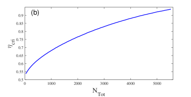
Figure 4: (a) Phase sensitivity $\Delta\phi$ versus photon losses in both arms $\eta_{a}$ and $\eta_{b}$, where $g=2$, $r=1$, $\left|\alpha\right|^{2}={e^{2r}}/{4}$. (b) The critical $\eta_{\mathrm{cri}}$ as a function of the total mean photon number inside the interferometer $N_{\mathrm{Tot}}$ where $g=2$, and $\eta_{a}$=$\eta_{b}$. Given a $N_{\mathrm{Tot}}$, the phase sensitivity $\Delta\phi$ beat the SQL when $\eta>\eta_{\mathrm{cri}}$.

Figure 5: Phase sensitivity $\Delta\phi$ versus photon losses $\eta$ and phase diffusion $\beta$ in both arms, where $g=2$, $r=1$, $\left|\alpha\right|^{2}={e^{2r}}/{4}$. SQL and HL denote the standard quantum limit and Heisenberg limit, respectively.

Substituting those optimal results $\gamma_{opt,i}^{\prime}$ and $\lambda_{opt}$ into $\mathcal{C}_{Q}$, the minimal $\mathcal{C}_{Q}$ is given by

$$\mathcal{C}_{\phi}=\frac{\widetilde{\mathcal{C}}_{Q}(\beta_{a}^{2}+\beta_{b}^{2})}{8\widetilde{\mathcal{C}}_{Q}\beta_{a}^{2}\beta_{b}^{2}+\beta_{a}^{2}+\beta_{b}^{2}},$$ (33)

and the corresponding phase sensitivity is

$$\Delta\phi\geq\sqrt{\frac{1}{\widetilde{\mathcal{C}}_{Q}}+\frac{8\beta_{a}^{2}\beta_{b}^{2}}{\beta_{a}^{2}+\beta_{b}^{2}}}.$$ (34)

The phase sensitivity shows the decoherence effect on the phase estimation, which is dependent on the photon loss coefficients $\eta_{i}$, and the phase diffusion noise coefficients $\beta_{i}$ ($i=a,b$). When the phase diffusion noise coefficients $\beta_{a}=\beta_{b}=0$, the above Eq. (34) can reduce to the result of only photon loss exists Gong17

$$\Delta\phi\geq\sqrt{1/\widetilde{\mathcal{C}}_{Q}}.$$ (35)

On the other hand, when the photon loss coefficients $\eta_{a}=\eta_{b}=0$, the result reduces to

$$\Delta\phi\geq\sqrt{1/\mathcal{F}_{Q}+8\beta_{a}^{2}\beta_{b}^{2}/(\beta_{a}^{2}+\beta_{b}^{2})}.$$ (36)

It also coincides with bound obtained in Ref. Escher12 when $\beta_{a}=\beta_{b}=\beta$. If $\eta_{i}=0$ and $\beta_{i}=0$ ($i=a,b$), we can recover the result of lossless case $\Delta\phi\geq\sqrt{1/\mathcal{F}_{Q}}$.

Considering a coherent light ($\alpha=\left|\alpha\right|e^{i\theta_{\alpha}}$) combined with a single-mode squeezed vacuum light ($|0,\varsigma\rangle$ with $\varsigma=r\exp(i\theta_{\varsigma})$ is the squeezing parameter) input, and $g$ describing the strength in NBS process, we analyze the phase sensitivity numerically. Only considering the effect of phase diffusion, the phase sensitivity as a function of mean total photon number $N_{\mathrm{Tot}}$ with different phase diffusion coefficients is shown in Fig. 3(a), where the SQL and HL denote the standard quantum limit and Heisenberg limit, respectively. The optimal sensitivity of phase estimation could still beat the SQL when $\beta<\beta_{\mathrm{cri}}$ with the subscript “cri” stands for critical value. The critical $\beta_{\mathrm{cri}}$ is dependent on the total mean photon number, and the $\beta_{\mathrm{cri}}$ versus the $N_{\mathrm{Tot}}$ is shown in Fig. 3(b). Only considering the effect of photon losses, the phase sensitivity as a function of photon losses in both arms $\eta_{a}$ and $\eta_{b}$ is shown in Fig. 4(a), and the $\eta_{\mathrm{cri}}$ versus the $N_{\mathrm{Tot}}$ in Fig. 4(b). The SU(1,1) interferometer can tolerate $10\%$ the photon loss when $N_{\mathrm{Tot}}<4500$. The phase sensitivity as a function of photon losses $\eta$ ($\eta_{a}=\eta_{b}=\eta)$ and phase diffusion $\beta$ ($\beta_{a}=\beta_{b}=\beta$) in both arms is shown in Fig. 5. It is demonstrated that the phase precision estimation is more tolerant with loss of light field compared with phase diffusion.

IV Conclusions

In conclusion we have studied the effects of decoherence on the phase sensitivity in an SU(1,1) interferometer. Based on the generalized phase transform including phase diffusion coefficients, we derived the phase sensitivity of an SU(1,1) interferometer in the presence of phase diffusion and photon losses simultaneously. The loss of light field and phase diffusion degraded the measure precision, and we have given the critical values where the phase sensitivity below the SNL in the presence of phase diffusion or photon losses.

V Acknowledgements

This work is supported by the National Key Research Program of China under Grant No. 2016YFA0302001 and NSFC Grants No. 11474095, No. 91536114, No. 11574086, No. 11654005, and Natural Science Foundation of Shanghai No. 17ZR1442800, and the Shanghai Rising-Star Program 16QA1401600.

References

- (1) C. W. Helstrom, Quantum Detection and Estimation Theory (Academic, New York, 1976).
- (2) A. S. Holevo, Probabilistic and Statistical Aspects of Quantum Theory (North-Holland, Amsterdam, 1982).
- (3) C. M. Caves, Quantum-mechanical noise in an interferometer, Phys. Rev. D 23, 1693(1981)
- (4) S. L. Braunstein and C. M. Caves, Statistical distance and the geometry of quantum states, Phys. Rev. Lett. 72, 3439 (1994).
- (5) S. L. Braunstein, C. M. Caves, and G. J. Milburn, Generalized uncertainty relations: Theory, examples, and Lorentz invariance, Ann. Phys. 247, 135 (1996).
- (6) H. Lee, P. Kok, and J. P. Dowling, A quantum Rosetta stone for interferometry, J. Mod. Opt. 49, 2325 (2002).
- (7) V. Giovannetti, S. Lloyd, and L. Maccone, Quantum Metrology, Phys. Rev. Lett. 96, 010401 (2006).
- (8) M. Zwierz, C. A. Pérez-Delgado, and P. Kok, General Optimality of the Heisenberg Limit for Quantum Metrology, Phys. Rev. Lett. 105, 180402 (2010).
- (9) V. Giovannetti, S. Lloyd, and L. Maccone, Quantum-Enhanced Measurements: Beating the Standard Quantum Limit, Science 306, 1330 (2004).
- (10) V. Giovannetti, S. Lloyd, and L. Maccone, Advances in quantum metrology, Nat. photon. 5, 222 (2011).
- (11) G. Tóth and I. Apellaniz, Quantum metrology from a quantum information science perspective, J. Phys. A 47, 424006 (2014).
- (12) C. L. Degen, F. Reinhard, and P. Cappellaro, Quantum sensing, Rev. Mod. Phys. 89, 035002 (2017).
- (13) B. P. Abbott et al. (LIGO Scientific Collaboration and Virgo Collaboration), Observation of Gravitational Waves from a Binary Black Hole Merger, Phys. Rev. Lett. 116, 061102 (2016).
- (14) B. Yurke, S. L. McCall, and J. R. Klauder, SU(2) and SU(1,1) interferometers, Phys. Rev. A 33, 4033 (1986).
- (15) W. N. Plick, J. P. Dowling, and G. S. Agarwal, Coherent-light-boosted, sub-shot noise, quantum interferometry, New J. Phys. 12, 083014 (2010).
- (16) J. Jing, C. Liu, Z. Zhou, Z. Y. Ou, and W. Zhang, Realization of a nonlinear interferometer with parametric amplifiers, Appl. Phys. Lett. 99, 011110 (2011).
- (17) F. Hudelist, J. Kong, C. Liu, J. Jing, Z. Y. Ou, and W. Zhang, Quantum metrology with parametric amplifier-based photon correlation interferometers, Nat. Commun. 5, 3049 (2014).
- (18) W. Du, J. Jia, J. F. Chen, Z. Y. Ou, and W. Zhang, Absolute sensitivity of phase measurement in an SU(1,1) type interferometer, Opt. Lett. 43, 1051 (2018).
- (19) C. Gross, T. Zibold, E. Nicklas, J. Estève, and M. K. Oberthaler, Nonlinear atom interferometer surpasses classical precision limit, Nature (London) 464, 1165 (2010).
- (20) J. Peise, B. Lücke, L. Pezzè, F. Deuretzbacher, W. Ertmer, J. Arlt, A. Smerzi, L. Santos, and C. Klempt, Interaction-free measurements by quantum Zeno stabilization of ultracold atoms, Nat. Commun. 6, 6811 (2015).
- (21) M. Gabbrielli, L. Pezzè, and A. Smerzi, Spin-Mixing Interferometry with Bose-Einstein Condensates, Phys. Rev. Lett. 115, 163002 (2015).
- (22) D. Linnemann, H. Strobel, W. Muessel, J. Schulz, R. J. Lewis-Swan, K. V. Kheruntsyan, and M. K. Oberthaler, Quantum-Enhanced Sensing Based on Time Reversal of Nonlinear Dynamics, Phys. Rev. Lett. 117, 013001 (2016).
- (23) S. Lemieux, M. Manceau, P. R. Sharapova, O. V. Tikhonova, R. W. Boyd, G. Leuchs, and M. V. Chekhova, Engineering the Frequency Spectrum of Bright Squeezed Vacuum via Group Velocity Dispersion in an SU(1,1) Interferometer, Phys. Rev. Lett. 117, 183601 (2016).
- (24) M. Manceau, G. Leuchs, F. Khalili, and M. Chekhova, Detection Loss Tolerant Supersensitive Phase Measurement with an SU(1,1) Interferometer, Phys. Rev. Lett. 119, 223604 (2017).
- (25) B. Chen, C. Qiu, S. Chen, J. Guo, L. Q. Chen, Z. Y. Ou, and W. Zhang, Atom-Light Hybrid Interferometer, Phys. Rev. Lett. 115, 043602 (2015).
- (26) J. Jacobson, G. Björk, and Y. Yamamoto, Quantum limit for the atom-light interferometer, Appl. Phys. B 60, 187-191 (1995).
- (27) S. A. Haine, Quantum Metrology in Open Systems: Dissipative Cramer-Rao Bound, Phys. Rev. Lett. 112, 120405 (2014).
- (28) S. S. Szigeti, B. Tonekaboni, W. Y. S. Lau, S. N. Hood, and S. A. Haine, Squeezed-light-enhanced atom interferometry below the standard quantum limit, Phys. Rev. A 90, 063630 (2014).
- (29) S. A. Haine and W. Y. S. Lau, Generation of atom-light entanglement in an optical cavity for quantum enhanced atom interferometry, Phys. Rev. A 93, 023607 (2016).
- (30) Z.-D. Chen, C.-H. Yuan, H.-M. Ma, D. Li, L. Q. Chen, Z. Y. Ou, and W. Zhang, Effects of losses in the atom-light hybrid SU(1,1) interferometer, Opt. Express 24, 17766 (2016).
- (31) Sh. Barzanjeh, D. P. DiVincenzo, and B. M. Terhal, Dispersive qubit measurement by interferometry with parametric amplifiers, Phys. Rev. B 90, 134515 (2014).
- (32) B. E. Anderson, P. Gupta, B. L. Schmittberger, T. Horrom, C. Hermann-Avigliano, K. M. Jones, and P. D. Lett, Phase sensing beyond the standard quantum limit with a variation on the SU(1,1) interferometer, Optica 4, 752 (2017).
- (33) B. E. Anderson, B. L. Schmittberger, P. Gupta, K. M. Jones, and P. D. Lett Optimal phase measurements with bright- and vacuum-seeded SU(1,1) interferometers, Phys. Rev. A 95, 063843 (2017)
- (34) P. Gupta, B. L. Schmittberger, B. E. Anderson, K. M. Jones, and P. D. Lett, Optimized phase sensing in a truncated SU(1,1) interferometer, Opt. Express 26, 000391 (2017).
- (35) Z. Y. Ou, Enhancement of the phase-measurement sensitivity beyond the standard quantum limit by a nonlinear interferometer, Phys. Rev. A 85, 023815 (2012).
- (36) A. M. Marino, N. V. Corzo Trejo, and P. D. Lett, Effect of losses on the performance of an SU(1,1) interferometer, Phys. Rev. A 86, 023844 (2012).
- (37) D. Li, C.-H. Yuan, Z. Y. Ou, and W. Zhang, The phase sensitivity of an SU (1, 1) interferometer with coherent and squeezed-vacuum light, New J. Phys. 16, 073020 (2014).
- (38) D. Li, B. T. Gard, Y. Gao, C.-H. Yuan, W. Zhang, H. Lee, and J. P. Dowling, Phase sensitivity at the Heisenberg limit in an SU(1,1) interferometer via parity detection, Phys. Rev. A 94, 063840 (2016).
- (39) D. Li, C.-H. Yuan, Y. Yao, W. Jiang, M. Li, and W. Zhang, Effects of loss on the phase sensitivity with parity detection in an SU(1,1) interferometer, J. Opt. Soc. Am. B 35, 1080 (2018).
- (40) Q.-K. Gong, D. Li, C.-H. Yuan, Z. Y. Ou, W. Zhang, Phase estimation of phase shifts in two arms for an SU(1,1) interferometer with coherent and squeezedvacuum states, Chin. Phys. B 26, 094205 (2017).
- (41) R. Demkowicz-Dobrzanski, U. Dorner, B. J. Smith, J. S. Lundeen, W. Wasilewski, K. Banaszek, and I. A. Walmsley, Quantum phase estimation with lossy interferometers, Phys. Rev. A 80, 013825 (2009).
- (42) R. Demkowicz-Dobrzanski, J. Kolodynski, and M. Guta, The elusive Heisenberg limit in quantum-enhanced metrology, Nat. Commun. 3, 1063 (2012).
- (43) D. W. Berry, Michael J. W. Hall, and H. M. Wiseman, Stochastic Heisenberg Limit: Optimal Estimation of a Fluctuating Phase, Phys. Rev. Lett. 111, 113601 (2013).
- (44) R. Chaves, J. B. Brask, M. Markiewicz, J. Kołodynski, and A. Acin, Noisy Metrology beyond the Standard Quantum Limit, Phys. Rev. Lett. 111, 120401 (2013).
- (45) W. Dur, M. Skotiniotis, F. Frowis, and B. Kraus, Improved Quantum Metrology Using Quantum Error Correction, Phys. Rev. Lett. 112, 080801 (2014).
- (46) E. M. Kessler, I. Lovchinsky, A. O. Sushkov, and M. D. Lukin, Quantum Error Correction for Metrology, Phys. Rev. Lett. 112, 150802 (2014).
- (47) S. Alipour, M. Mehboudi, and A. T. Rezakhani, Quantum Metrology in Open Systems: Dissipative Cramer-Rao Bound, Phys. Rev. Lett. 112, 120405 (2014).
- (48) D. Brivio, S. Cialdi, S. Vezzoli, B. T. Gebrehiwot, M. G. Genoni, S. Olivares, and M. G. A. Paris, Experimental estimation of one-parameter qubit gates in the presence of phase diffusion, Phys. Rev. A 81, 012305(2010).
- (49) M. G. Genoni, S. Olivares, and M. G. A. Paris, Opical Phase Estimation in the Presence of Phase Diffusion, Phys. Rev. Lett. 106, 153603 (2011).
- (50) M. G. Genoni, S. Olivares, D. Brivio, S. Cialdi, D. Cipriani, A. Santamato, S. Vezzoli, and M. G. A. Paris, Opical interferometry in the presence of large phase diffusin, Phys. Rev. A 85, 043817 (2012).
- (51) B. M. Escher, R. L. de Matos Filho, L. Davidovich, General framework for estimating the ultimate precision limit in noisy quantum-enhanced metrology, Nature Phys. 7, 406 (2011).
- (52) B. M. Escher, L. Davidovich, N. Zagury, and R. L. de Matos Filho, Quantum Metrological limits via a variational approach, Phys. Rev. Lett. 109, 190404 (2012).
- (53) X. M. Feng, G. R. Jin, and W. Yang, Quantum interferometry with binary-outcome measurements in the presence of phase diffusion, Phys. Rev. A 90, 013807(2014).
- (54) C. Sparaciari, S. Olivares and M. G. A. Paris, Gaussian-state interferometry with passive and active elements, Phys. Rev. A 93 023810 (2016).
- (55) J. Trapani, B. Teklu, S. Olivares, and M. G. A. Paris, Quantum phase communication channels in the presence of static and dynamical phase diffusion, Phys. Rev. A 92, 012317 (2015).
- (56) M. D. Vidrighin, G. Donati, M. G. Genoni, X.-M. Jin, W. St. Kolthammer, M. S. Kim, A. Datta, M. Barbieri, and I. A. Walmsley, Joint estimation of phase and phase diffusion for quantum metrology, Nat. Commun. 5, 3532 (2014).
- (57) M. Altorio, M. G. Genoni, M. D. Vidrighin, F. Somma, and M. Barbieri, Weak measurements and the joint estimation of phase and phase diffusion, Phys. Rev. A 92, 032114 (2015).
- (58) M. Zwierz and H. Wiseman, Precision bounds for noisy nonlinear quantum metrology, Phys. Rev. A 89, 022107 (2014).
- (59) E. Giese, S. Lemieux, M. Manceau, R. Fickler, and R.W. Boyd, Phase sensitivity of gain-unbalanced nonlinear interferometers, Phys. Rev. A 96, 053863 (2017).
- (60) Q.-K. Gong, X.-L. Hu, D. Li, C.-H. Yuan, Z. Y. Ou, and W. Zhang, Intramode correlations enhanced phase sensitivities in an SU(1,1) interferometer, Physical Review A 96, 033809 (2017).
- (61) L. Pezzè and A. Smerzi, Quantum theory of phase estimation, in Atom Interferometry, edited by G. M. Tino and M. A. Kasevich, Proceedings of the International School of Physics “Enrico Fermi”, Varenna, Course 188 (IOS Press, Amsterdam, 2014), pp. 691–741.