Scattering of co-current surface waves on an analogue black hole

Abstract

We report on what is to our knowledge the first scattering experiment of surface waves on an accelerating transcritical flow, which in the Analogue Gravity context is described by an effective spacetime with a black-hole horizon. This spacetime has been probed by an incident co-current wave, which partially scatters into an outgoing counter-current wave on each side of the horizon. The measured scattering amplitudes are compatible with the predictions of the hydrodynamical theory, where the kinematical description in terms of the effective metric is exact.

Recent years have witnessed an explosion of interest in Analogue Gravity Barceló et al. (2011); Barceló (2019). This newly emergent field builds on Unruh’s insight of 1981 Unruh (1981) that, using the mathematical equivalence between wave propagation in curved spacetimes on the one hand and in condensed matter systems on the other, one can realize an analogue black hole in the laboratory and test Hawking’s prediction that black holes emit radiation Hawking (1974, 1975). In this context, an analogue black hole is engendered by an accelerating flow which becomes supersonic. The point where the flow crosses the speed of sound is the (acoustic) horizon for sound waves, in analogy with the (event) horizon for light at a gravitational black hole. Because wave propagation close to the horizon is equivalent in the two cases, the Hawking effect, which is derived from purely kinematical considerations, should be present also in the analogue system. This prediction has been the main driving force behind the Analogue Gravity program since its inception, with experimental studies in a wide range of physical systems, such as nonlinear optics Philbin et al. (2008); Belgiorno et al. (2010); Ciret et al. (2016); Drori et al. (2019), exciton-polaritons Nguyen et al. (2015) and Bose-Einstein condensates Steinhauer (2014, 2016); de Nova et al. (2019).

Surface waves on fluids provide another example of an analogue system Schützhold and Unruh (2002); Rousseaux (2013). Consider a rectangular flume oriented along the $x$-direction, containing a water flow which is independent of the transverse coordinate $y$. In the shallow-water limit $kh\ll 1$ ( $k$ being the wave vector and $h$ the depth), the free-surface deformation $\delta h$ behaves like the canonical momentum of a minimally coupled massless scalar field propagating in the $(2+1)$-dimensional spacetime metric

$$\mathrm{d}s^{2}=c^{2}\left[c^{2}\,\mathrm{d}t^{2}-\left(\mathrm{d}x-v\,\mathrm{d}t\right)^{2}-\mathrm{d}y^{2}\right]\,.$$ (1)

The metric (5) describes a “spacetime fluid” flowing in the $x$-direction with velocity $v(x)$ and variable “speed of light” $c(x)$. The $x$-oriented null geodesics of the metric (5) are simply described by ${\rm d}x/{\rm d}t=v\pm c$. For waves, this equation gives the motion of characteristics, and is equivalent to the following (linear) dispersion relation whenever $v$ and $c$ are constant:

$$\Omega=\omega-vk=\pm ck\,,$$ (2)

where $\Omega$ is the “co-moving” frequency measured in the rest frame of the fluid, while $\omega$ is the Doppler-shifted frequency measured in the lab frame. We assume the flow is from left to right, i.e. $v>0$, so that the plus and minus signs in Eq. (6) respectively define waves engaged in co- and counter-current propagation. In particular, the total velocity of counter-current waves is $v-c$, which can take either sign. A transcritical flow has $v-c=0$ somewhere. This point is the (analogue) horizon, marking the boundary between subcritical ($v-c<0$) and supercritical ($v-c>0$) regions. Accelerating flows which pass from subcritical to supercritical have specifically an analogue black-hole horizon, with counter-current waves outgoing on either side.

Matters are complicated by the prefactor of $c^{2}$ in Eq. (5), which can be thought of as a conformal factor relating the effective metric to the simpler one in square brackets. In an appropriate coordinate system, this term generates an effective potential Anderson et al. (2013, 2014) which scatters co- into counter-current waves and vice versa. The two outgoing counter-current waves can thus be excited by a co-current wave sent in by a wave maker.

There have been a number of recent experiments aimed at realizing and probing analogue spacetimes of the form (5) seen by surface waves Rousseaux et al. (2008, 2010); Weinfurtner et al. (2011); Euvé et al. (2015, 2016); Torres et al. (2017); Euvé and Rousseaux (2017). However, these have tended to remain far from the ideal case originally envisaged by Unruh. Most importantly, in none of these experiments was a transcritical flow achieved, so that the corresponding analogue spacetimes did not contain horizons . In such cases, the nontrivial scattering processes analogous to those involved in the Hawking effect can exist only thanks to the presence of short-wave dispersion, which requires the singling out of a preferred frame and thus breaks the analogue of Lorentz invariance. The relevant scattering amplitudes cannot be derived from the spacetime description; in particular, those pertaining to the analogue of the Hawking process do not generally follow the Planck law so central to Hawking’s thermal prediction Michel and Parentani (2014); Robertson et al. (2016). Furthermore, all experiments in 1D settings have focused on decelerating flows, which in the transcritical case would yield analogue white-hole horizons. These are convenient for scattering experiments as they convert incident hydrodynamical (long-wavelength) waves, which are easy to excite, into outgoing dispersive (short-wavelength) waves, which are easy to measure. However, this means that the kinematics of the outgoing modes are not describable using the effective metric formalism alone. Things are further complicated by the ubiquity of undulations (i.e., zero-frequency solutions with finite wave vector) on the downstream sides of decelerating flows Coutant and Parentani (2014); Michel et al. (2018).

I Experimental setup

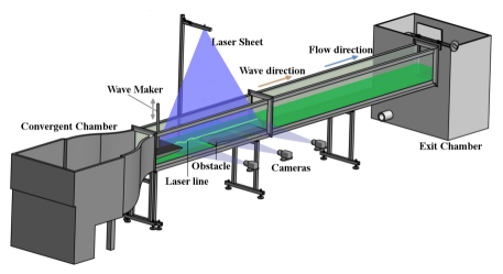
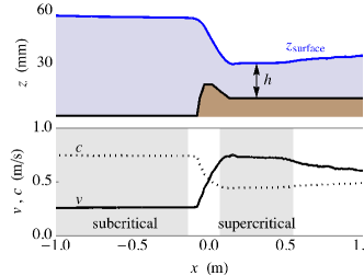
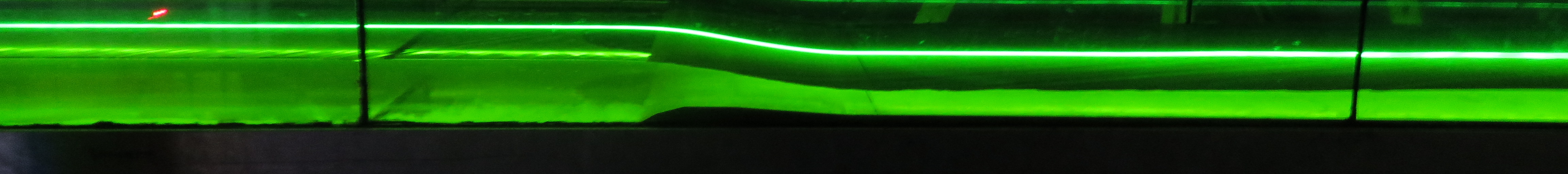
Figure 1: Experimental setup. On the left is an illustration of the flume, showing the flow direction and the position of the wave maker. On the right are shown: upper) the obstacle on the bottom of the flume and the stationary profile of the surface, found by averaging $z_{\rm surface}(t,x)$ over time; lower) the corresponding profiles of $v$ and $c$ (according to Eqs. (3)), with the near-homogeneous regions (where the plane wave decomposition is performed) shaded. The bottom panel shows a photo of the flume, where one sees clearly the variation of the water depth and the laser illuminating the midline. The distance between the black vertical bars is $1\,\mathrm{m}$.

We have realized, at Institut Pprime of the University of Poitiers, a transcritical flow in a flume analogous to a black-hole spacetime, and performed a scattering experiment on this flow that can be described in terms of the effective metric. The experimental setup and the stationary flow profile are illustrated in Figure 1. A flume of length $7\,{\rm m}$ and width $39\,{\rm cm}$ is used, and on the bottom of the flume is placed a dedicated obstacle with $x$-dependent height, designed in accordance with well-known principles of hydraulics (set out pedagogically by Walker in Walker (1981)). The current is maintained by a PCM Moineau pump. The convergent chamber, containing a honeycomb structure, removes practically all boundary-layer effects and macro-vortices, producing a flow velocity profile that (in the upstream region) is approximately constant in both the vertical and tranverse directions. At a given flow rate, which is measured by a Promag 55S flow meter to within an error of $0.5\%$, the stationary flow that results has a particular mean depth profile $h(x)$. The presence of surface waves causes the instantaneous depth to vary in time around this mean.

Measurements were made of the instantaneous vertical position $z_{\rm surface}(t,x)$ of the water surface along the midline of the flume. A laser sheet, produced by a laser diode (at wavelength $473\,\mathrm{nm}$ and power $100\,\mathrm{mW}$) and a Powell lens, was shone through the water, to which had been added fluorescein dye Weinfurtner et al. (2011); Euvé et al. (2016). At a suitable concentration ($\sim 20\,{\rm g}/{\rm m}^{3}$), the dye absorbs the blue laser light and emits green light near the surface (up to a depth of $\sim 5\,\mathrm{mm}$). The laser line produced (see Fig. 1) was recorded by three cameras at regular intervals of $\Delta t\sim 0.1\,{\rm s}$, for a total duration of $800\,{\rm s}$. A subpixel detection algorithm yielded the surface height at each time at a series of positions separated by the constant spacing $\Delta x=3.4\,{\rm mm}$. From this was subtracted the known height profile of the obstacle in order to get the instantaneous water depth $h(t,x)$. The mean depth $h(x)$ is then found by averaging over time. Assuming the fluid to be irrotational and the surface quasi-flat (i.e. $\left|\partial_{x}z_{\rm surface}\right|\ll 1$), the flow velocity and wave speed are related to the mean depth by

$$v(x)=\frac{q}{h(x)}\,,\qquad c(x)=\sqrt{gh(x)}\,,$$ (3)

where $q$ is the (constant) flow rate per unit width (measured at $147.4\pm 0.7\,{\rm cm}^{2}/{\rm s}$) and $g=9.8\,\mathrm{m/s^{2}}$ is the acceleration due to gravity. As seen in the lower right panel of Fig. 1, the realized flow passes from subcritical to supercritical, thus engendering an analogue black-hole horizon at the point where $v=c$.

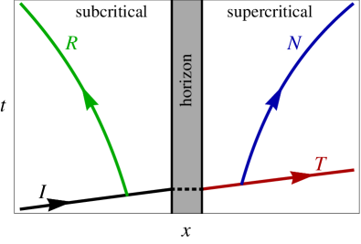
Figure 2: Space-time diagram of the scattering process, showing the wave characteristics involved in the scattering of an incident co-current wave (I, black) into a transmitted co-current wave (T, red), a reflected counter-current wave (R, green) and a transmitted counter-current wave (N, blue). The flow is from left to right, passing from subcritical to supercritical.

Surface waves were stimulated by a plunging-type wave maker placed upstream from the obstacle. We performed a series of experimental runs for a range of frequencies at three different wave maker amplitudes: $A_{\rm wm}=0.25\,{\rm mm}$, for which $f\in\left[0.55\,,\,1.2\right]\,{\rm Hz}$; $A_{\rm wm}=0.5\,{\rm mm}$, for which $f\in\left[0.2\,,\,1.0\right]\,{\rm Hz}$; and $A_{\rm wm}=1.0\,{\rm mm}$, for which $f\in\left[0.2\,,\,0.5\right]\,{\rm Hz}$. The elongated shape of the wave maker allows the displacement of a large volume of fluid, producing long waves of small amplitude which have a negligible effect on the mean flow (we estimate the relative change in the Froude number $v/c$ due to the passage of the wave to be at most $2\%$). The co-current waves thus excited were incident on the horizon; this is analogous to sending matter in towards a black hole from far away. The scattering process is illustrated in Figure 2. Much of the wave was simply transmitted (with amplitude $T$), while scattering at the effective potential also produced a reflected wave (with amplitude $R$) and a counter-current wave in the supercritical region (with amplitude $N$).

II Main results

Focusing on the near-homogeneous regions (shaded gray in the lower right panel of Fig. 1), we assumed that the waveform in each is a sum of two plane waves, and were thus able to extract best-fit values for the amplitudes and wave vectors – see the Supplemental Material (SM) SM for details. The subcritical region staying relatively flat over a considerable distance, we could take a longer near-homogeneous region there, and we thus expect greater accuracy of the results pertaining to this side.

Dispersion relation. In Figure 3 are shown the best-fit values of the wave vectors in each of the near-homogeneous regions. Immediately, we see that (with the exception of three outliers on the bottom right of the lower panel) each region shows two branches of the dispersion relation with clear signs of the derivative ${\rm d}f/{\rm d}k$ (where $f=\omega/2\pi$), this being the sign of the group velocity of the corresponding wave. We thus conclude that we have one ingoing and one outgoing wave on the subcritical side, while on the supercritical side we instead have two outgoing waves. This is indicative of the presence of an analogue black-hole horizon: it shows that $v-c$ changes sign when moving from one near-homogeneous region to the other.

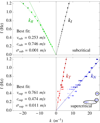
Figure 3: Measured wave vectors. The various colors correspond to the modes of Fig. 2, while the three different shadings of data points correspond to different wave maker amplitudes: $A_{\rm wm}=0.25\,{\rm mm}$ (dark), $0.5\,{\rm mm}$ (medium) and $1\,{\rm mm}$ (light). Circled points are outliers. The solid curves show theoretical dispersion relations fitted to the linear behavior of Eq. (6) for $kh\ll 1$. The fitted values of $v$ and $c$ in each region, as well as their error $\sigma$, are indicated. The dotted line in the upper panel shows the full theoretical dispersion relation (see footnote 2) with $h_{\rm sub}$ given by $c_{\rm sub}$ via Eqs. (3).

Also shown are fits to the theoretical dispersion relations. As already mentioned, these take the linear form of Eq. (6) in the shallow-water regime $kh\ll 1$, so we may use the lower range of $k$ to find the best-fit values of $v$ and $c$ in each region. These are given explicitly in Fig. 3; $v$ is about $3\%$ smaller than predicted by Eqs. (3) (see the discussion below concerning the flow rate $q$), while $c$ agrees with the prediction to within $0.1\%$.. Moreover, since we expect the flow to be uniform in the subcritical region, we may use the best-fit values of $v$ and $c$ to find the corresponding values of $q$ and $h$ through Eqs. (3). Not only is the extracted water depth there, $h_{\rm sub}=56.7\pm 0.1\,{\rm mm}$, consistent with the profile of Fig. 1, but it also agrees with the observed deviations from the linear dispersion relation . The fitted value of the flow rate is $q_{\rm fit}=143.6\pm 0.3\,{\rm cm}^{2}/{\rm s}$, which differs quite significantly from the measured value of $147.4\pm 0.7\,{\rm cm}^{2}/{\rm s}$. This is most likely due to the non-uniformity of the flow speed in the vertical direction. Indeed, numerical simulations indicate that $v$ tends to decrease slightly near the surface, which would explain why $q_{\rm fit}$ is smaller than the measured value (see SM SM ).

On the supercritical side, the extracted wave vectors are considerably less accurate, having larger error bars and appearing to oscillate around the expected linear curves. While this is partly due to the reduction of the window size with respect to that in the subcritical region, it should be noted that there is a considerable degree of noise in the supercritical region. Even so, only four data points (which have been circled in Fig. 3) are clear outliers. $v$ and $c$ are found to be about $5$ and $7\%$ larger, respectively, than those predicted by Eqs. (3). This discrepancy is likely due to the non-uniformity of the flow after passing over the obstacle, and is reminiscent of a similar observation made in the downstream region in Ref. Euvé et al. (2015).

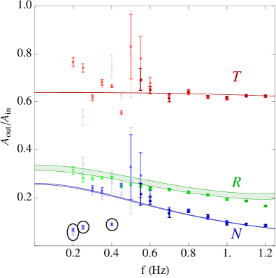
Figure 4: Measured scattering amplitudes. The colors and shadings correspond to the same outgoing branches and wave maker amplitudes as in Fig. 3. The colored lines are theoretical predictions, and have finite widths corresponding to the uncertainty in $h_{\rm sub}$. The amplitudes of the outliers circled in Fig. 3 are also circled here.

Scattering coefficients. In Figure 4 are shown the three outgoing wave amplitudes in units of the incident wave amplitude. Also shown are predictions extracted from the wave equation associated with the metric (5) . As expected, the most accurate of the scattering amplitudes (in terms of the smallness of the error bars) is $R$, this having been extracted purely from the subcritical region. The amplitudes relating to the supercritical region are less accurately determined, with much larger error bars than $R$. This is due both to the smaller available window size where the flow is approximately homogeneous, and also to the presence of a significant amount of noise, which seems to be related to the occurrence of side wakes (see SM SM ). However, the extracted scattering amplitudes still compare favorably with the hydrodynamical theory.

In summary, we have extracted the dispersion relations and scattering amplitudes pertaining to the interaction of an incident co-current surface wave with an analogue black hole. The dispersion relations show a total of three outgoing modes, implying the presence of an analogue horizon. Except for the high-frequency sector of the $R$-branch, the modes relevant to the scattering process are in the non-dispersive regime where the effective metric description is valid, and the measured scattering amplitudes are compatible with its predictions.

Following in the spirit of Weinfurtner et al. (2011); Euvé et al. (2016), a future goal of this type of (classical) analogue model is the observation of (the stimulated version of) the Hawking process, whereby the squared norm of the relevant scattering coefficient takes the form of a thermal spectrum. The absence of transcriticality in previous experiments prevents the direct verification of the Hawking-Unruh thermal prediction, which can only be applied when a horizon is present. Our setup makes this possible in two ways. Firstly, one could consider a stationary background like that used in this paper. This can only be achieved by exploiting dispersion and sending in a short-wavelength mode , but these are difficult to excite in practice. The second possibility is to consider a time-dependent background in which an initially subcritical flow develops a supercritical region. In this context one can study, in particular, the scattering of initial long-wavelength countercurrent modes into final long-wavelength countercurrent modes (i.e., those labeled as $R$ and $N$ in the present work), thus avoiding the need to send in a dispersive wave. This case is reminiscent of that originally studied by Hawking Hawking (1974, 1975), of a star collapsing to form a black hole.

Acknowledgments

We would like to thank Romain Bellanger, Laurent Dupuis and Jean-Marc Mougenot for their help concerning the experimental aspects of this work. We also thank Roberto Balbinot, Ulf Leonhardt, and particularly Florent Michel, Renaud Parentani and Thomas Philbin for their careful reading of and constructive comments on a previous version of the manuscript. This work was supported by the French National Research Agency through Grant No. ANR-15-CE30-0017-04 associated with the project HARALAB, by the University of Poitiers (ACI UP on Wave-Current Interactions 2013–2014), by the Interdisciplinary Mission of CNRS which funded the linear motor of the wave maker in 2013, and by the University of Tours in a joint grant with the University of Poitiers (ARC Poitiers-Tours 2014–2015). It benefited from the support of the project OFHYS of the CNRS 80 Pprime initiative in 2019. It was partially supported by the Spanish Mineco grants FIS2014-57387-C3-1-P and FIS2017-84440-C2-1-P, the Generalitat Valenciana project SEJI/2017/042 and the Severo Ochoa Excellence Center Project SEV-2014-0398.

Appendix A Supplemental material

A.1 Theoretical background

In this section we provide more theoretical details on the effective metric description of the scattering of surface waves, with particular emphasis on the scattering process examined in the main paper (referred to here as the Letter).

A.1.1 Wave equation

In the shallow-water limit $h/\lambda\ll 1$ (where $h$ is the water depth and $\lambda$ the wavelength), and assuming $\left|\partial_{x}z_{\rm surface}\right|\ll 1$ everywhere (where $z_{\rm surface}=h_{\rm obs}+h$ is the vertical position of the free surface, $h_{\rm obs}$ being the height of the obstacle), longitudinal surface waves on an inviscid, irrotational, two-dimensional flow obey the following wave equation Schützhold and Unruh (2002); Unruh (2013); Coutant and Parentani (2014):

$$\left[\left(\partial_{t}+\partial_{x}v\right)\left(\partial_{t}+v\partial_{x}\right)-\partial_{x}c^{2}\partial_{x}\right]\phi=0\,.$$ (4)

The scalar field $\phi$ is a perturbation of the velocity potential, i.e., $\Phi=\Phi_{0}+\phi$ where $\vec{v}=-\nabla\Phi$. The free-surface deformation is given by $\delta h=-\frac{1}{g}\left(\partial_{t}+v\partial_{x}\right)\phi$ (where $g=9.8\,{\rm m}/{\rm s}^{2}$ is the acceleration due to gravity). The position-dependent parameters $v$ and $c$ are determined by the background flow; specifically, $v$ is the longitudinal component of the local flow velocity and $c$ is the local speed of surface waves with respect to the fluid. Equation (4) is precisely the Klein-Gordon wave equation in curved spacetime, $\Box\phi=0$ (see Barceló et al. (2011) for details), for the longitudinal modes of a massless scalar field propagating in the $(2+1)$-dimensional spacetime metric 

$$\mathrm{d}s^{2}=c^{2}\left[c^{2}\,\mathrm{d}t^{2}-\left(\mathrm{d}x-v\,\mathrm{d}t\right)^{2}-\mathrm{d}y^{2}\right]\,,$$ (5)

already given in Eq. (1) of the Letter. As mentioned there, the characteristics of wave equation (4) are precisely the $x$-directed null geodesics of the metric (5), and are simply described by ${\rm d}x/{\rm d}t=v\pm c$, which in the wave picture is equivalent to the dispersion relation

$$\Omega=\omega-vk=\pm ck$$ (6)

whenever $v$ and $c$ are constant. While $\omega$ is just the Doppler shifted frequency due to the motion of the fluid, stationarity in the frame of the flume ensures that $\omega$ (rather than $\Omega$) is conserved by any linear scattering process. Assuming for definiteness that $v>0$, dispersion relation (6) defines co-current and counter-current waves (respectively, those taking the $+$ and $-$ sign on the right-hand side of Eq. (6)), and a horizon where $v-c=0$ splits the counter-current waves into two distinct branches localized on either side of the horizon.

A.1.2 Conservation laws

The conserved energy associated with Eq. (4) is (up to an overall prefactor)

$$E=\int\mathrm{d}x\left\{\left|\partial_{t}\phi\right|^{2}+\left(c^{2}-v^{2}\right)\left|\partial_{x}\phi\right|^{2}\right\}\,.$$ (7)

From this expression, it is readily apparent that wherever the flow becomes supercritical, it is possible for the integrand (i.e., the energy density) to be negative. Treating $v$ and $c$ as constant and directly substituting $\phi=A\,{\rm exp}\left(ikx-i\omega t\right)$, with $\omega$ and $k$ satisfying dispersion relation (6), we find that the energy density of such a plane wave is (proportional to) $\omega\Omega\left|A\right|^{2}$. The signs of $\omega$ and $\Omega$ are opposite whenever the flow is strong enough to reverse the total velocity of the wave, which is precisely the case for counter-current waves in the supercritical region. These waves thus have negative energy with respect to the stationary background: their presence reduces the total energy of the system. Crucially, they share their lab frequency $\omega$ with several waves of positive energy, yielding the possibility of anomalous scattering involving both positive- and negative-energy waves.

At fixed $\omega$, the wave form is stationary and infinitely extended, and the most useful conservation law is that for the energy flux, defined as the energy density times the group velocity $v_{g}={\rm d}\omega/{\rm d}k=v\pm c$, where the $+$ ($-$) corresponds to co- (counter-) current waves. It is straightforward to show that, for a plane wave, the energy flux is proportional to $\pm\omega^{2}c\left|A\right|^{2}$; therefore, co- (counter-) current waves always contribute positively (negatively) to the total energy flux. The total energy flux must be constant in $x$; for, if it were not, the energy density would be changing somewhere, contradicting the stationarity of the wave form. It is thus appropriate to consider normalized plane waves $\phi^{(N)}$ of fixed energy flux, so that a general plane wave $\phi$, and the corresponding free-surface deformation $\delta h=-\frac{1}{g}\left(\partial_{t}+v\partial_{x}\right)\phi$, can be written as

$$\phi = \mathcal{A}\,\phi^{(N)} = \frac{\mathcal{A}}{\sqrt{\omega}}\,\frac{{\rm exp}\left(ikx-i\omega t\right)}{\sqrt{\omega\,c}}\,,$$

$$\delta h = \mathcal{A}\,\delta h^{(N)} = \frac{\mathcal{A}}{\sqrt{\omega}}\,i\frac{\Omega}{g}\,\frac{{\rm exp}\left(ikx-i\omega t\right)}{\sqrt{\omega\,c}}\,.$$ (8)

The contribution of this wave to the total energy flux is proportional to $\pm\left|\mathcal{A}\right|^{2}$.

Equations (8) generalize readily to dispersive models Corley and Jacobson (1996); Macher and Parentani (2009):

$$\phi = \mathcal{A}\,\phi^{(N)} = \frac{\mathcal{A}}{\sqrt{\omega}}\,\frac{{\rm exp}\left(ikx-i\omega t\right)}{\sqrt{\left|\Omega\,v_{g}\right|}}\,,$$

$$\delta h = \mathcal{A}\,\delta h^{(N)} = \frac{\mathcal{A}}{\sqrt{\omega}}\,i\frac{\Omega}{g}\,\frac{{\rm exp}\left(ikx-i\omega t\right)}{\sqrt{\left|\Omega\,v_{g}\right|}}\,,$$ (9)

where $v_{g}={\rm d}\omega/{\rm d}k$ is the group velocity. In the non-dispersive limit, these reduce to Eqs. (8). Most important for our purposes is the factor of $\sqrt{\left|\Omega/v_{g}\right|}$ multiplying the plane waves of $\delta h$, since at fixed $\omega$ this is the part of the normalizing prefactor which varies from one mode to another.

A.1.3 Scattering of co-current waves

As mentioned in the Letter, the simple kinematical description given above is complicated by the prefactor $c^{2}$ in Eq. (5). In the present context, the significance of this term stems from the fact that it is the transverse component of the metric, i.e., the coefficient of ${\rm d}y^{2}$ in Eq. (5). Although we are interested in waves which do not depend on $y$, local inhomogeneities in this term can scatter co- into counter-current waves and vice versa, thus playing the role of an effective potential .

Our experiment aims to probe the structure of the spacetime induced by a transcritical flow through the scattering of incident co-current waves by the effective potential. The scattering process is illustrated in the space-time diagram shown in Figure 2 of the Letter . A co-current wave is incident from the subcritical side; this is analogous to sending matter in towards a black hole from far away. Since the effective potential vanishes at the horizon, the entire process can be decomposed into two time-ordered scattering events, each localized to one side of the horizon. First, the incident wave partially scatters at the effective potential outside the black hole, producing a (positive-energy) counter-current wave that propagates back towards the subcritical region. This process is described by a reflection coefficient $\mathcal{R}$. The unreflected part of the incident wave then crosses the horizon, and is partially scattered by the effective potential inside the black hole. This time, a counter-current wave of negative energy is produced, and propagates in the same direction as the transmitted wave, i.e. falling further into the supercritical region. Relating the outcome of this process to the incident wave requires two scattering coefficients, $\mathcal{N}$ and $\mathcal{T}$. Imposing equality of the total energy flux on either side of the horizon, we find $1-\left|\mathcal{R}\right|^{2}=\left|\mathcal{T}\right|^{2}-\left|\mathcal{N}\right|^{2}$, or equivalently,

$$\left|\mathcal{T}\right|^{2}+\left|\mathcal{R}\right|^{2}-\left|\mathcal{N}\right|^{2}=1\,.$$ (10)

This is the unitarity relation, an algebraic constraint on the scattering coefficients which encodes total energy conservation. The fact that one of the scattering coefficients counts negatively towards this relation indicates that anomalous scattering is taking place.

A.1.4 Calculation of scattering coefficients for a given flow profile

In the non-dispersive model described by wave equation (4), the normalized scattering amplitudes can be calculated directly by re-expressing (4) in terms of WKB-like solutions (in the spirit of Baird (1970); Massar and Parentani (1998)). Let us define

$$W_{\omega}^{U}(x)=\frac{\mathrm{exp}\left(i\omega\,U(x)\right)}{\omega\,\sqrt{c(x)}}\,,\qquad W_{\omega}^{V}(x)=\frac{\mathrm{exp}\left(i\omega\,V(x)\right)}{\omega\,\sqrt{c(x)}}\,,$$ (11)

where

$$U(x)=\int^{x}\frac{dx^{\prime}}{v(x^{\prime})-c(x^{\prime})}\,,\qquad V(x)=\int^{x}\frac{dx^{\prime}}{v(x^{\prime})+c(x^{\prime})}\,.$$ (12)

In homogeneous regions $W_{\omega}^{U}$ and $W_{\omega}^{V}$ describe the counter- and co-current waves, respectively. Moreover, the factors of $\left(\omega\sqrt{c(x)}\right)^{-1}$ ensure that their energy flux is constant (cf. Eqs. (8)), so they are physically allowable solutions as far as energy conservation is concerned. However, they are not exact solutions of Eq. (4), because we have not yet accounted for the mixing of the the two modes by inhomogeneities in $c$. To include this mixing, we introduce $x$-dependent amplitudes $\mathcal{A}_{\omega}^{U}$ and $\mathcal{A}_{\omega}^{V}$ such that

$$\phi_{\omega}(x) = \mathcal{A}_{\omega}^{U}(x)\,W_{\omega}^{U}(x)+\mathcal{A}_{\omega}^{V}(x)\,W_{\omega}^{V}(x)\,,$$ (13a)

$$\partial_{x}\phi_{\omega}(x) = i\omega\,U^{\prime}(x)\,\mathcal{A}_{\omega}^{U}(x)\,W_{\omega}^{U}(x)$$ (13b)

$$\qquad\quad+i\omega\,V^{\prime}(x)\,\mathcal{A}_{\omega}^{V}(x)\,W_{\omega}^{V}(x)\,.$$

Equation (4) can now be re-expressed as a pair of coupled first-order differential equations for the amplitudes:

$$\partial_{x}\left[\begin{array}[]{c}\mathcal{A}_{\omega}^{U}\\ \mathcal{A}_{\omega}^{V}\end{array}\right]=\frac{1}{2}\,\frac{\partial_{x}c}{c}\,\left[\begin{array}[]{cc}0&e^{-i\omega(U(x)-V(x))}\\ e^{i\omega(U(x)-V(x))}&0\end{array}\right]\left[\begin{array}[]{c}\mathcal{A}_{\omega}^{U}\\ \mathcal{A}_{\omega}^{V}\end{array}\right]\,.$$ (14)

It is straightforward to show that Eq. (14) implies

$$\partial_{x}\left[\left|\mathcal{A}_{\omega}^{V}\right|^{2}-\left|\mathcal{A}_{\omega}^{U}\right|^{2}\right]=0\,,$$ (15)

which, given that $W_{\omega}^{U}$ and $W_{\omega}^{V}$ are already normalized, is exactly the expression for conservation of energy flux. The waveform corresponding to the scattering of incident co-current waves is found by setting $\mathcal{A}_{\omega}^{U}=0$ arbitrarily close to the horizon, i.e., by imposing the non-existence of waves emanating from the horizon. We then integrate Eq. (14) out into the asymptotic regions – this is done separately on the subcritical and supercritical sides of the flow, since $W_{\omega}^{U}$ must be separately defined on each side of the horizon – and the appropriate normalization is achieved by setting the amplitude of the incident wave to $1$. The amplitudes $\mathcal{A}_{\omega}^{V}$ and $\mathcal{A}_{\omega}^{U}$ in the homogeneous regions are then identified with $\mathcal{T}$, $\mathcal{R}$ and $\mathcal{N}$, satisfying Eq. (10).

As already stated, the free surface deformation $\delta h$ is related to $\phi$ via $\delta h=-\frac{1}{g}\left(\partial_{t}+v\partial_{x}\right)\phi$. So, if $\phi$ is given by Eq. (13a), $\delta h$ is given by

$$\delta h_{\omega}(x) = \frac{i\omega}{g}\left[\frac{c(x)}{c(x)-v(x)}\,\mathcal{A}_{\omega}^{U}(x)\,W_{\omega}^{U}(x)\right.$$ (16)

$$\qquad\left.+\frac{c(x)}{c(x)+v(x)}\,\mathcal{A}_{\omega}^{V}(x)\,W_{\omega}^{V}(x)\right]$$

$$= \frac{i}{g}\left[\frac{\sqrt{c(x)}}{c(x)-v(x)}\,\mathcal{A}_{\omega}^{U}(x)\,e^{i\omega\,U(x)}\right.$$

$$\qquad\left.+\frac{\sqrt{c(x)}}{c(x)+v(x)}\,\mathcal{A}_{\omega}^{V}(x)\,e^{i\omega\,V(x)}\right]\,.$$

This expression yields the necessary conversion factors between the normalized amplitudes and the “bare” amplitudes extracted directly from the data. Using a cursive style for the normalized amplitudes (as in Eq. (10)) and a non-cursive style for the “bare” amplitudes (as in the Letter), we have

$$R = \frac{c_{\rm sub}+v_{\rm sub}}{c_{\rm sub}-v_{\rm sub}}\,\mathcal{R}\,,$$

$$T = \sqrt{\frac{c_{\rm sup}}{c_{\rm sub}}}\,\frac{c_{\rm sub}+v_{\rm sub}}{c_{\rm sup}+v_{\rm sup}}\,\mathcal{T}\,,$$

$$N = -\sqrt{\frac{c_{\rm sup}}{c_{\rm sub}}}\,\frac{c_{\rm sub}+v_{\rm sub}}{v_{\rm sup}-c_{\rm sup}}\,\mathcal{N}\,.$$ (17)

On the other hand, generalizing to the dispersive case using Eqs. (9), these become

$$R = \sqrt{\left|\frac{\Omega_{R}}{\Omega_{\rm in}}\right|\left|\frac{v_{g,{\rm in}}}{v_{g,R}}\right|}\,\mathcal{R}\,,$$

$$T = \sqrt{\left|\frac{\Omega_{T}}{\Omega_{\rm in}}\right|\left|\frac{v_{g,{\rm in}}}{v_{g,T}}\right|}\,\mathcal{T}\,,$$

$$N = -\sqrt{\left|\frac{\Omega_{N}}{\Omega_{\rm in}}\right|\left|\frac{v_{g,{\rm in}}}{v_{g,N}}\right|}\,\mathcal{N}\,.$$ (18)

The expressions in Eqs. (17) are simply the restrictions of Eqs. (18) to the non-dispersive case.

It is interesting and useful to note that, in the limit $\omega\to 0$ (where the dispersive and non-dispersive normalizations agree), the normalized amplitude $\mathcal{R}$ and the ratio of normalized amplitudes $\mathcal{N}/\mathcal{T}$ are simply related to the limiting values of $c$ within their respective regions (calculated using methods developed in Anderson et al. (2015)):

$$\left|\mathcal{R}\right|^{2}\to\left(\frac{c_{\rm sub}-c_{\rm hor}}{c_{\rm sub}+c_{\rm hor}}\right)^{2}\,,\qquad\left|\frac{\mathcal{N}}{\mathcal{T}}\right|^{2}\to\left(\frac{c_{\rm sup}-c_{\rm hor}}{c_{\rm sup}+c_{\rm hor}}\right)^{2}\,,$$ (19)

where $c_{\rm sub}$ and $c_{\rm sup}$ are the values of $c$ in the sub- and supercritical regions, respectively, and $c_{\rm hor}$ is its value at the horizon. Notice that Eqs. (19) are in accordance with the fact that no mode mixing occurs if $c$ is constant.

A.2 Data analysis

In this section, we provide a detailed account of the data analysis used to extract the results presented in the Letter. This includes technical information and further results complementary to those already presented.

A.2.1 Background flow

An original two-dimensional free-surface flow code was developed in order to simulate numerically the transcritical flow studied experimentally in the Letter. A projection method is applied to the incompressible variable density Navier-Stokes equations to decouple velocity and pressure unknowns. Away from the interfaces (water-air and obstacle-water), partial differential operators (divergence, gradient, Laplacian operator) and nonlinear terms are discretized on a fixed Cartesian grid using standard second-order finite difference approximations. Several techniques are used to account for the presence of the two interfaces while avoiding the generation of conformal meshes. An Immersed Boundary Method Bouchon et al. (2012) enforces the no-slip boundary condition on the rigid obstacle and the free surface evolution is tackled with the Level-Set technique Osher and Sethian (1988).

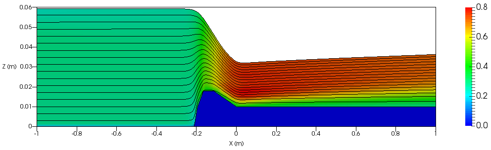
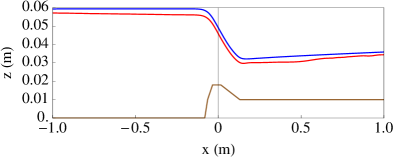
Figure 5: Numerical results pertaining to the stationary background flow, which is assumed homogeneous in the transverse direction. In the upper panel is shown the magnitude of the flow velocity on a color scale (in units of ${\rm m}/{\rm s}$), with its direction lying along the streamlines shown in black. In the lower panel are shown the numerically calculated free surface (blue) and that found experimentally after averaging $\delta h(x,t)$ in time (red). The apparent discrepancy averages at $2.60\,{\rm mm}$, which is close to the pixel size used in the simulation ($\Delta z=2.75\,{\rm mm}$).

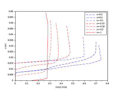
Figure 6: The longitudinal component of the flow velocity as a function of the vertical coordinate $z$, at a series of fixed longitudinal coordinates $x$.

In Figures 5 and 6 are shown the results of the numerical calculation for the flow across the obstacle, and with a total flow rate close to that used in the experiment. This assumes that the system is homogeneous in the transverse direction, so that the flow velocity has no dependence on or component along $y$; boundary effects due to the walls of the channel are thus neglected. In Fig. 5, the upper panel shows the magnitude of the flow on a color scale (its direction being indicated by the streamlines in black), while the lower panel shows the numerically derived water depth (in blue) on the same graph as the experimental time-averaged water depth (in red). There is a small apparent discrepancy with a spatial average of $2.60\,{\rm mm}$, which is close to the pixel size used in the simulation ($\Delta z=2.75\,{\rm mm}$). Even so, the qualitative similarity between the two can be appreciated. Figure 6 explicitly plots the longitudinal component of the flow velocity as a function of depth at several values of the longitudinal coordinate $x$.

We see that the numerically calculated flow is very close to laminar in the upstream region, before the flow crosses the obstacle. The standard expressions $v=q/h$ and $c=\sqrt{gh}$ (Eqs. (3) of the Letter) are thus expected to work very well there. Moreover, we can expect to be sensitive to small deviations from the idealized theoretical model. We have already seen that the dispersive corrections to the wave vectors of the reflected waves are visible at high frequencies (see Fig. 3 of the Letter). We have also noted in the Letter a discrepancy between the measured value of the flow rate $q$, and the fitted value of $q$ assuming the validity of $v=q/h$ in the subcritical region. The solid curve in Fig. 6 indicates that, while $v$ is essentially constant over most of the depth, there is a slight decrease as the free surface is approached. Since it is the surface value of $v$ that enters the effective metric for surface waves, this behavior near the surface should engender a small decrease in $q_{\rm fit}$ with respect to the measured $q$. Indeed, in the Letter we find that $q_{\rm fit}$ is smaller than $q$ by about $3\%$. We thus believe that the decrease of $v(z)$ near the surface is responsible for the discrepancy between $q$ and $q_{\rm fit}$.

The numerical results also indicate that we should expect somewhat larger discrepancies from the standard predictions for $v$ and $c$ once we enter the supercritical (downstream) region, for there the variation of the flow velocity with depth is more significant. This is again what is observed: the extracted value of $v$ is considerably larger than $q/h$, which is consistent with the appearance of a significant boundary layer at the bottom of the flow where $v$ is smaller than it is near the surface.

It is important to emphasize the two-dimensional nature of the numerical calculations used to produce Fig. 5. That is, the flow velocity is assumed to be completely independent of the transverse direction. This means that any boundary effects due to the walls of the flume have not been taken into account. One such effect, visible to the naked eye, is shown in the photo of Fig. 7: a quasi-stationary wake pattern emanating from the walls of the flume in the supercritical region. By “quasi-stationary” we mean that it is not strictly time-dependent, with positions of the crests and troughs showing a considerable amount of jitter that is noticeable by eye and which will contribute to the free-surface fluctuations $\delta h(t,x)$. This is likely the source of the increased noise level in the supercritical region.

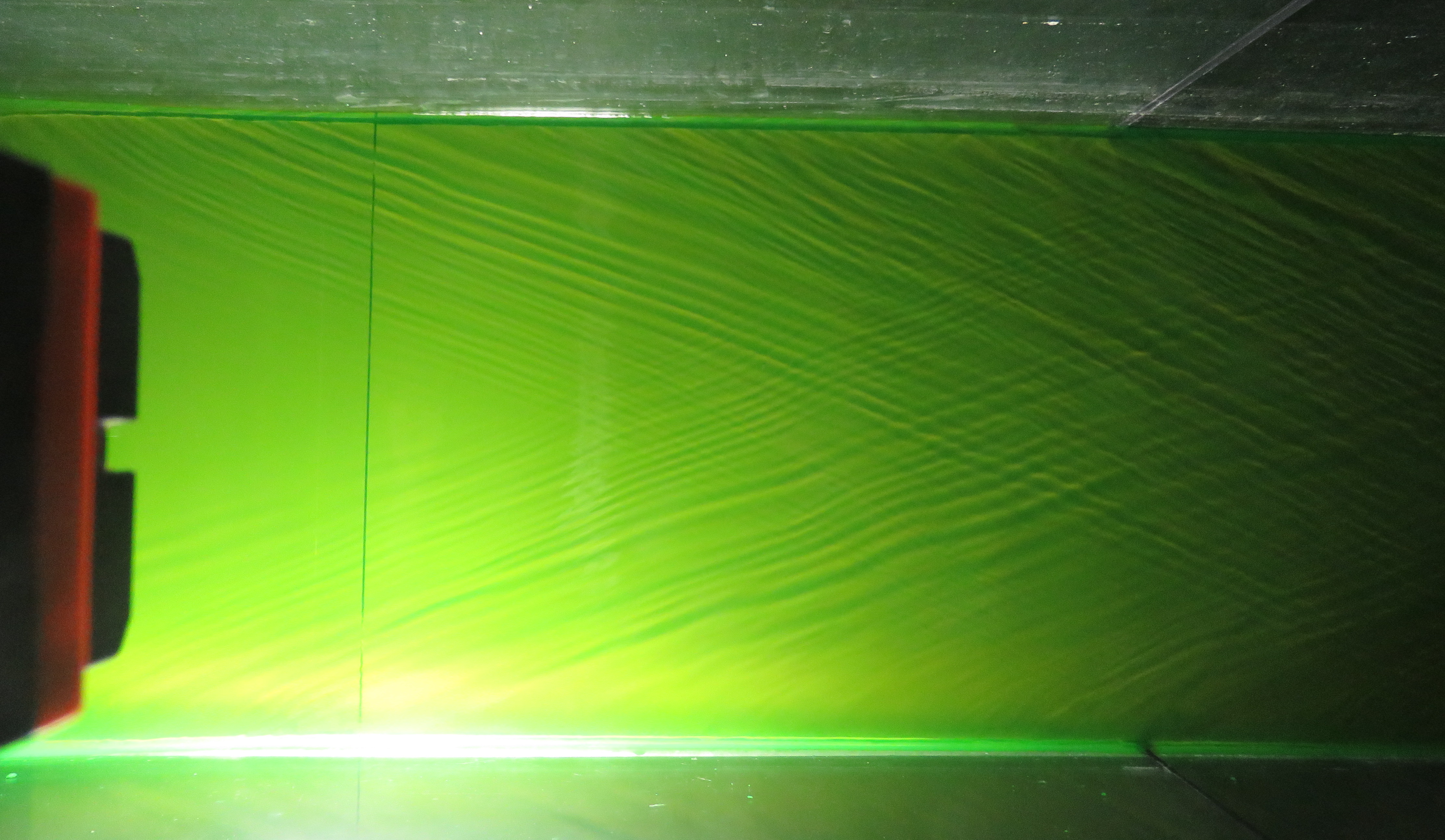
Figure 7: Aerial view of the water surface in the supercritical region. The side wakes – emanations from the walls of the channel – are clearly visible.

A.2.2 Extracting wave vectors and amplitudes from the experimental data

Measurements are made of the free-surface deformation, $\delta h(t,x)$. We suppose that in each run this can be written as

$$\!\!\!\!\!\!\!\!\delta h(t,x) = {\rm Re}\left\{\delta h_{\omega}(x)\,e^{-i\omega t}\right\}+{\rm noise}$$ (20)

$$= \frac{1}{2}\,\delta h_{\omega}(x)\,e^{-i\omega t}+\frac{1}{2}\,\delta h^{\star}_{\omega}(x)\,e^{i\omega t}+{\rm noise}\,,$$

where $\omega$ is the frequency of stimulation by the wave maker. $\delta h_{\omega}(x)$ can thus be extracted by taking the Fourier component at frequency $\omega$:

$$\delta h_{\omega}(x)\approx\frac{2}{N}\sum_{j=1}^{N}e^{i\omega t_{j}}\delta h\left(t_{j}\,,\,x\right)\,.$$ (21)

Here, the $t_{j}$ are the discrete times at which the data has been recorded. The total number of such times is $N_{t}=8192$, for a total duration of $800\,{\rm s}$. Examples of the extracted waveform, at two different frequencies, are shown in Fig. 8.

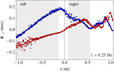
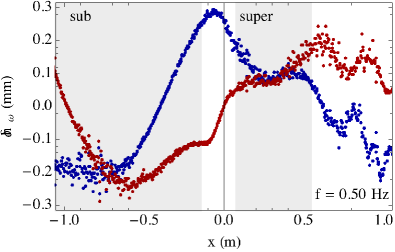
Figure 8: Extracted waveform $\delta h_{\omega}(x)$, found by Fourier transforming the data in time at the stimulation frequency of the wave maker. The chosen runs are at frequencies $0.25\,{\rm Hz}$ (upper panel) and $0.5\,{\rm Hz}$ (lower panel), with a wave maker amplitude $A_{\rm wm}=0.5\,{\rm mm}$. Blue and red data points correspond to the real and imaginary parts, respectively, of $\delta h_{\omega}(x)$. The sub- and supercritical regions, where fitting to a sum of two plane waves is performed, are shaded.

With the complex waveform $\delta h_{\omega}(x)$ having been extracted, we focus our attention on the near-homogeneous regions on either side of the horizon. There, the dispersion relation $\omega(k)$ is essentially independent of position and there should be almost no scattering between the various waves. Therefore, the complex waveform should be expressible as a sum of plane waves:

$$\delta h_{\omega,{\rm hom}}(x)=A_{1}\,e^{ik_{1}x}+A_{2}\,e^{ik_{2}x}\,.$$ (22)

Since we wish to fit the wave vectors as well as the amplitudes, the fit is performed using the Mathematica function “NonlinearModelFit”, which also provides estimates for the errors in the fitting parameters. The procedure used both for the fitting and the error estimation can be illustrated as in Fig. 9. We consider a section of the $\left(k_{1},\,k_{2}\right)$-plane, and for each point on this plane we may perform a linear fit of the amplitudes $A_{1}$ and $A_{2}$ at the given values of $k_{1}$ and $k_{2}$. This fit is precisely defined via the minimization of $\chi^{2}$ (the sum of the squared residuals):

$$\chi^{2}=\sum_{j=1}^{N_{x}}\frac{\left|\delta h_{\omega}\left(x_{j}\right)-\delta h_{\omega,{\rm hom}}\left(x_{j}\right)\right|^{2}}{\sigma^{2}}\,,$$ (23)

where we have assumed that the error $\sigma$ is independent of position. For each $\left(k_{1},\,k_{2}\right)$, minimizing $\chi^{2}$ returns the best fit values of $A_{1}$ and $A_{2}$. The error $\sigma$ is estimated by assuming the reduced $\chi^{2}$, i.e., $\chi^{2}$ per degree of freedom (here $\chi^{2}/\left(2N_{x}-6\right)$, an extra factor of $2$ appearing since the function is complex-valued), is equal to $1$ at the minimum. Shown in Fig. 9 are contour plots of the reduced $\chi^{2}$, and we clearly see a well-defined local minimum at some point $\left(k_{1},\,k_{2}\right)$. The errors on $k_{1}$ and $k_{2}$ are estimated by considering the contour where the reduced $\chi^{2}$ is equal to $2$ (shown in thick black in Fig. 9). As for any normal probability distribution, it is estimated that the actual $\left(k_{1},\,k_{2}\right)$ lies in the region bounded by this contour with a probability of about $68\%$, and the errors on $k_{1}$ and $k_{2}$ are just the projected widths of this region on the $k_{1}$- and $k_{2}$-axes.

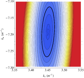
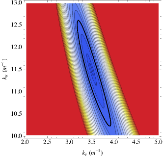
Figure 9: Reduced $\chi^{2}$ in the 2D wave vector plane, shown on a color scale. The values are shown for the run with $A_{\rm wm}=0.25\,{\rm mm}$ and $f=0.55\,{\rm Hz}$, in the subcritical region (left panel) and in the supercritical region (right panel). For each wave vector pair, $\left(k_{v},\,k_{u}\right)$, a linear fit of the wave amplitudes is performed and the reduced $\chi^{2}$ is extracted. The point where this reaches a minimum value (defined to be $1$) represents the best fit, while the locus where it increases to $2$ (indicated by the thick black contour) defines the standard error. The projections of this region onto each of the axes give the standard errors in $k_{v}$ and $k_{u}$ shown in Fig. 3 of the Letter.

Note that the errors on $k_{1}$ and $k_{2}$ defined by this ellipse will feed into the errors associated with the amplitudes; for, while the errors on the amplitudes for each fixed point $\left(k_{1},\,k_{2}\right)$ are defined by the standard linear fitting procedure and may not be especially large, the corresponding best fit values of the amplitudes may vary quite a lot over the length of the ellipse in the $\left(k_{1},\,k_{2}\right)$-plane. This variation must then be included in the error on the amplitudes, and may turn out to be the dominant contribution. This appears to be what happens when the errors on $T$ and $N$ become large around $f=0.5\,{\rm Hz}$ in Fig. 4 of the Letter: the region of the $\left(k_{1},\,k_{2}\right)$-plane where the wave vectors are likely to lie turns out to be rather long (see the right panel of Fig. 9), and the variation of $T$ and $N$ along it is rather large.

It is also to be noted that some trial and error is required when performing a nonlinear fit of the type described here, with the wave vectors being included as fitting parameters. This is because (unlike in a linear fit) a local minimum of $\chi^{2}$ is not uniquely defined, and is therefore not guaranteed to be a global minimum. We therefore look in the vicinity of the expected value of $\left(k_{v},\,k_{u}\right)$, and the minimum closest to it selected. That said, when working in the supercritical region, there are a few cases where a larger-than-expected value of $k_{u}$ appears to be unavoidable; these are the outliers circled in Fig. 3 of the Letter.

A.2.3 Comparing theoretical and measured scattering amplitudes

In Fig. 4 of the Letter, we have shown the “bare” (unnormalized) scattering amplitudes, extracted directly from the data since they are simply ratios of the measured outgoing wave amplitudes to that of the incident wave. In that case, the theoretical predictions yielded by Eq. (14) are converted into “bare” amplitudes using Eqs. (18); the conversion factors, which take dispersive corrections into account, are evaluated for the values of $v$ and $c$ extracted in Fig. 3 of the Letter. Here instead, we adopt the inverse approach (see Fig. 10): the normalized amplitudes directly calculated using Eq. (14) are shown, and the “bare” amplitudes extracted from the data are converted into normalized amplitudes according to the inverse forms of Eqs. (18). The conversion factors are once again dispersive and evaluated for the extracted $v$ and $c$, but for comparison we also show (with fainter data points) the results we would obtain using the non-dispersive conversion formulae of Eqs. (17). For clarity, the three scattering amplitudes are shown on separate panels, with the colors of the data points indicating the corresponding amplitude of the wave maker oscillations: $A_{\rm wm}=0.25\,{\rm mm}$ (blue), $0.5\,{\rm mm}$ (red) and $1\,{\rm mm}$ (green). In theory these should satisfy the unitarity relation (10), but since $\left|\mathcal{R}\right|^{2}$ and $\left|\mathcal{N}\right|^{2}$ are a lot smaller than $\left|\mathcal{T}\right|^{2}$, the sum on the left-hand side of (10) is indistinguishable from $\left|\mathcal{T}\right|^{2}$; we are thus unable to demonstrate that $\left|\mathcal{R}\right|^{2}$ and $\left|\mathcal{N}\right|^{2}$ contribute to the unitarity relation in the expected way.

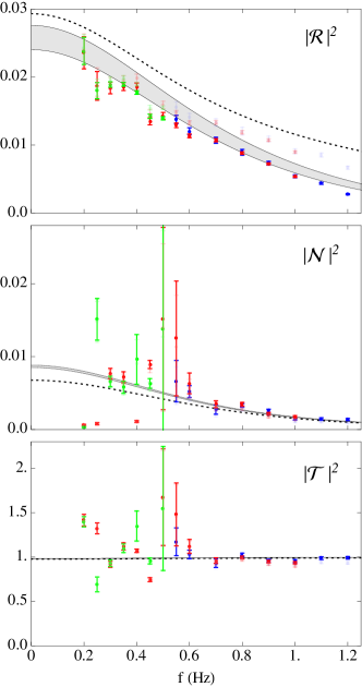
Figure 10: Normalized scattering amplitudes. The differently colored data points correspond to the different amplitudes of the wave maker: $A_{\rm wm}=0.25\,{\rm mm}$ (blue), $0.5\,{\rm mm}$ (red) and $1\,{\rm mm}$ (green). Normal shading of data points indicates the use of dispersive normalization factors, while light shading is for the results obtained when normalizing according to the non-dispersive theory. The dotted curves give the predictions of the hydrodynamical theory when using the standard expressions for $v$ and $c$ (Eqs. (3) of the Letter), while the gray shaded regions correspond to the predictions of the refined model using Eqs. (24).

For each scattering amplitude, two theoretical predictions are shown which differ in their description of the background. The dotted curves in Fig. 10 show the predictions when using the standard expressions for $v(x)$ and $c(x)$ given by Eqs. (3) of the Letter. Although these are not far from the observed values, there is a particularly noticeable discrepancy in the $\left|\mathcal{R}\right|^{2}$ coefficient. To try and improve the comparison between theory and experiment, we also consider the following expressions Coutant and Parentani (2014) :

$$\frac{1}{2}v^{2}(x)+gz_{\rm surface}(x) = \frac{1}{2}v_{\rm as}^{2}+gh_{\rm as}\,,$$

$$c^{2}(x) = gh_{\rm as}\frac{v_{\rm as}}{v(x)}\,.$$ (24)

The corresponding $v(x)$ and $c(x)$ are shown in Fig. 11, along with the standard profiles of Eqs. (3) of the Letter and the extracted values of $v$ and $c$ in the near-homogeneous regions. The asymptotic values $h_{\rm as}$ and $v_{\rm as}$ entering Eqs. (24) are taken to be those extracted in the subsonic region: $h_{\rm sub}=56.7\pm 0.1\,{\rm mm}$ and $v_{\rm sub}=25.3\pm 0.1\,{\rm cm}/{\rm s}$, with the errors on $h_{\rm sub}$ and $v_{\rm sub}$ allowing us to define a prediction “band” rather than a single well-defined curve. Interestingly, the profile of $v(x)$ given by Eqs. (24) is (unlike that of Eqs. (3) of the Letter) wholly consistent with the value of $v_{\rm sup}$ extracted in the supersonic region. By contrast, the profile of $c(x)$ is slightly further from the extracted value of $c_{\rm sup}$ than that given by Eqs. (3) of the Letter. It should be noted that $v(x)$ and $c(x)$ of Eqs. (24) are more sensitive to small changes of $z_{\rm surface}(x)$ in the subsonic region, and show a bit more variation there than Eqs. (3) of the Letter (a noticeable slope can be seen in Fig. 11). Therefore, when using Eq. (14) to produce theoretical scattering amplitudes, we stop the integration just outside the inhomogeneity engendered by the obstacle (specifically at $x=\pm 0.2\,{\rm m}$) .

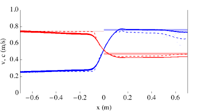
Figure 11: Profiles of $v$ (blue) and $c$ (red), according to Eqs. (3) of the Letter (dashed) and to Eqs. (24) of this Supplemental Material (solid). The shaded regions indicate the values of $v$ and $c$ extracted in the near-homogeneous regions (see Fig. 3 of the Letter).

Returning to Fig. 10, it is clear that the combination of using dispersive normalization factors to convert the “bare” amplitudes to normalized ones, and the use of Eqs. (24) for $v(x)$ and $c(x)$ rather than Eqs. (3) of the Letter, yields the most favorable comparison between theory and experiment. The respective differences are most noticeable in $\left|\mathcal{R}\right|^{2}$, which shows the greatest sensitivity both to dispersive normalization factors (as might have been expected) and to the precise forms of $v(x)$ and $c(x)$. The other amplitudes also show some improvement: $\left|\mathcal{N}\right|^{2}$ is rather insensitive to dispersion but at low frequencies is more compatible with the refined versions of $v(x)$ and $c(x)$, while $\left|\mathcal{T}\right|^{2}$ is rather insensitive to changes of the background but shows some improvement at high frequencies when dispersion is included in the normalization factors. Note that dispersion plays a minimal role here, entering only in the normalization factors but being absent from the predictions of the normalized scattering amplitudes. It thus seems to play little role in the scattering, at least until we reach the highest frequencies probed and we start to see the measured $\left|\mathcal{R}\right|^{2}$ falling further away from the theoretical prediction.

A.2.4 Background noise and harmonics

The fitting performed in deriving the results above assumes that the only element of $\delta h(t,x)$ is the linear perturbation oscillating at the stimulated frequency $\omega$, i.e. that $\delta h(t,x)=\mathrm{Re}\left\{\delta h_{\omega}(x)e^{-i\omega t}\right\}$. In fact, there are other contributions, and it is useful to be aware of them and their relative importance compared with the main signal.

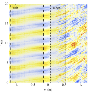
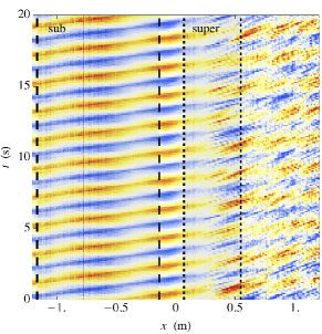
Figure 12: Space-time diagrams showing $\delta h(x,t)$ for two different experimental runs, with the wave maker frequency equal to $0.25\,{\rm Hz}$ (left panel) and $0.5\,{\rm Hz}$ (right panel), and the wave maker amplitude fixed at $0.5\,{\rm mm}$. $\delta h$ is plotted on a color scale as indicated by the color bar on the right (the values are in $\mathrm{mm}$). The black vertical lines correspond to the limits of the near-homogeneous regions on the subcritical (dashed) and supercritical (dotted) sides, as also illustrated in Fig. 1 of the Letter and in Fig. 8 of this Supplementary Material. On the subcritical side, the data is clean and regular, and in the right plot we can see variations of the amplitude of the oscillations due to interference between the incident and reflected waves. On the supercritical side, however, the data clearly becomes much noisier, and this growth appears to occur precisely in the near-homogeneous region delineated by the dotted vertical lines.

In Figure 12 are shown space-time diagrams plotting $\delta h(t,x)$, for frequencies $f=0.25\,{\rm Hz}$ (left panel) and $f=0.5\,{\rm Hz}$ (right panel) and a wave maker amplitude of $0.5\,{\rm mm}$. The sub- and supercritical near-homogeneous regions are delineated by the dashed and dotted vertical lines, respectively. Of particular notice is the noisy character of the data in the supercritical region, with this noise appearing to begin precisely in the near-homogeneous region where the fitting is performed. The data in the subcritical region is, by contrast, very clean and regular.

To investigate this further, in Figure 13 we show the squared magnitude of the time Fourier transforms of $\delta h(t,x)$, for several fixed values of $x$. To this end, the data is first divided into blocks of duration $100\,{\rm s}$ each, with the mean of $h(x)$ being calculated and subtracted in each block separately, and the squared magnitudes of the Fourier transforms are finally averaged over all eight blocks. The chosen values of $x$ are taken to be the edges of the windows defining the near-homogeneous regions. There is some background noise of roughly constant magnitude over all frequencies, and which has roughly the same value in both the subcritical region and the upstream edge of the supercritical region. However, by the time we reach the downstream edge of the supercritical region, this background noise has increased by between 1 and 2 orders of magnitude. This seems to be consistent with the higher degree of noise seen in the supercritical region in Fig. 12, and which emerges from within the near-homogeneous part of the supercritical region.

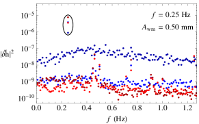
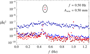
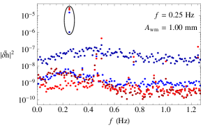
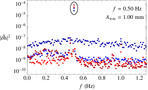
Figure 13: Time-Fourier transform of the free surface deformations at several fixed positions. The different positions are indicated by the variously colored dots: light and dark red are, respectively, the upstream and downstream edges of the subcritical region (delineated by the dashed vertical lines in Fig. 12); while light and dark blue are, respectively, the upstream and downstream edges of the supercritical region (delineated by the dotted vertical lines in Fig. 12). The left and right columns correspond to two different frequencies of the wave maker, while the upper and lower rows have two different amplitudes of the wave maker oscillations. In each plot the main signal, whose frequency is equal to that of the wave maker, is highlighted by a black oval, and we note that its strength is always greater than the background noise by at least an order of magnitude. Notably, while the other points have a comparable level of background noise, the downstream edge of the supercritical region shows noise which is about an order of magnitude greater. This illustrates the growth in the noise level over the supercritical region already noted in Fig. 12, and which may be due to the growth of side wakes (see Fig. 7 below). We also note that the pump frequency at $\sim 0.45\,\mathrm{Hz}$ can be seen in the background noise, except at the most downstream position where it has been obscured by the increased noise level.

We also note the occurrence of a signal at a well-defined frequency $\omega\approx 2.9\,{\rm Hz}$ (or $f\approx 0.45\,{\rm Hz}$), which occurs at all positions except the downstream edge of the supercritical region, where it is drowned out by the increased background noise. This frequency occurs for all stimulated frequencies and wave maker amplitudes, and we believe it to be characteristic of the vibrations of the water pump which maintains the background flow; indeed, this frequency shifts when the flow rate is changed, as would be expected if it were due to the water pump. Interestingly, the measured values of $\left|R\right|^{2}$ and $\left|N\right|^{2}$ show signs of resonant behavior near $f=0.45\,{\rm Hz}$, and this could be because the stimulated wave comes into resonance with the pump frequency, which could quite drastically alter the scattering process in the vicinity of that frequency.

Finally, we note that harmonics are visible in Fig. 13, but these are quite clearly smaller than the main signal by several orders of magnitude. We conclude that the signal is essentially linear in nature, and we can neglect the harmonics in predicting and explaining the observations.

References

- Barceló et al. (2011) Carlos Barceló, Stefano Liberati, and Matt Visser, “Analogue gravity,” Living Rev. Relativ. 14, 3 (2011).
- Barceló (2019) Carlos Barceló, “Analogue black-hole horizons,” Nat. Phys. 15, 210 (2019).
- Unruh (1981) William G. Unruh, “Experimental black-hole evaporation?” Phys. Rev. Lett. 46, 1351 (1981).
- Hawking (1974) Stephen W. Hawking, “Black hole explosions?” Nature 248, 30 (1974).
- Hawking (1975) Stephen W. Hawking, “Particle creation by black holes,” Comm. Math. Phys. 43, 199 (1975).
- Philbin et al. (2008) Thomas G. Philbin, Chris Kuklewicz, Scott Robertson, Stephen Hill, Friedrich König, and Ulf Leonhardt, “Fiber-optical analog of the event horizon,” Science 319, 1367 (2008).
- Belgiorno et al. (2010) Francesco Belgiorno, Sergio L. Cacciatori, Matteo Clerici, Vittorio Gorini, Giovanni Ortenzi, Luca Rizzi, Eleonora Rubino, Vera G. Sala, and Daniele Faccio, “Hawking radiation from ultrashort laser pulse filaments,” Phys. Rev. Lett. 105, 203901 (2010).
- Ciret et al. (2016) Charles Ciret, François Leo, Bart Kuyken, Gunther Roelkens, and Simon-Pierre Gorza, “Observation of an optical event horizon in a silicon-on-insulator photonic wire waveguide,” Opt. Express 24, 114 (2016).
- Drori et al. (2019) Jonathan Drori, Yuval Rosenberg, David Bermudez, Yaron Silberberg, and Ulf Leonhardt, “Observation of stimulated Hawking radiation in an optical analogue,” Phys. Rev. Lett. 122, 010404 (2019).
- Nguyen et al. (2015) Hai Son Nguyen, Dario Gerace, Iacopo Carusotto, Daniele Sanvitto, Elisabeth Galopin, Aristide Lemaître, Isabelle Sagnes, Jacqueline Bloch, and Alberto Amo, “Acoustic black hole in a stationary hydrodynamic flow of microcavity polaritons,” Phys. Rev. Lett. 114, 036402 (2015).
- Steinhauer (2014) Jeff Steinhauer, “Observation of self-amplifying Hawking radiation in an analogue black-hole laser,” Nature Physics 10, 864 (2014).
- Steinhauer (2016) Jeff Steinhauer, “Observation of quantum Hawking radiation and its entanglement in an analogue black hole,” Nature Physics 12, 959 (2016).
- de Nova et al. (2019) Juan Ramón Muñoz de Nova, Katrine Golubkov, Victor I. Kolobov, and Jeff Steinhauer, “Observation of thermal Hawking radiation and its temperature in an analogue black hole,” Nature 569, 688 (2019).
- Schützhold and Unruh (2002) Ralf Schützhold and William G. Unruh, “Gravity wave analogues of black holes,” Phys. Rev. D 66, 044019 (2002).
- Rousseaux (2013) Germain Rousseaux, “The basics of water waves theory for analogue gravity,” in Analogue Gravity Phenomenology: Analogue Spacetimes and Horizons, from Theory to Experiment, edited by Daniele Faccio, Francesco Belgiorno, Sergio Cacciatori, Vittorio Gorini, Stefano Liberati, and Ugo Moschella (Springer International Publishing, Cham, 2013) pp. 81–107.
- Anderson et al. (2013) Paul R. Anderson, Roberto Balbinot, Alessandro Fabbri, and Renaud Parentani, “Hawking radiation correlations in Bose-Einstein condensates using quantum field theory in curved space,” Phys. Rev. D 87, 124018 (2013).
- Anderson et al. (2014) Paul R. Anderson, Roberto Balbinot, Alessandro Fabbri, and Renaud Parentani, “Gray-body factor and infrared divergences in 1D BEC acoustic black holes,” Phys. Rev. D 90, 104044 (2014).
- Rousseaux et al. (2008) Germain Rousseaux, Christian Mathis, Philippe Maïssa, Thomas G. Philbin, and Ulf Leonhardt, “Observation of negative-frequency waves in a water tank: a classical analogue to the Hawking effect?” New J. Phys. 10, 053015 (2008).
- Rousseaux et al. (2010) Germain Rousseaux, Philippe Maïssa, Christian Mathis, Pierre Coullet, Thomas G. Philbin, and Ulf Leonhardt, “Horizon effects with surface waves on moving water,” New J. Phys. 12, 095018 (2010).
- Weinfurtner et al. (2011) Silke Weinfurtner, Edmund W. Tedford, Matthew C. J. Penrice, William G. Unruh, and Gregory A. Lawrence, “Measurement of stimulated Hawking emission in an analogue system,” Phys. Rev. Lett. 106, 021302 (2011).
- Euvé et al. (2015) Léo-Paul Euvé, Florent Michel, Renaud Parentani, and Germain Rousseaux, “Wave blocking and partial transmission in subcritical flows over an obstacle,” Phys. Rev. D 91, 024020 (2015).
- Euvé et al. (2016) Léo-Paul Euvé, Florent Michel, Renaud Parentani, Thomas G. Philbin, and Germain Rousseaux, “Observation of noise correlated by the Hawking effect in a water tank,” Phys. Rev. Lett. 117, 121301 (2016).
- Torres et al. (2017) Theo Torres, Sam Patrick, Antonin Coutant, Mauricio Richartz, Edmund W. Tedford, and Silke Weinfurtner, “Rotational superradiant scattering in a vortex flow,” Nature Physics 13, 833 (2017).
- Euvé and Rousseaux (2017) Léo-Paul Euvé and Germain Rousseaux, “Classical analogue of an interstellar travel through a hydrodynamic wormhole,” Phys. Rev. D 96, 064042 (2017).
- Michel and Parentani (2014) Florent Michel and Renaud Parentani, “Probing the thermal character of analogue Hawking radiation for shallow water waves?” Phys. Rev. D 90, 044033 (2014).
- Robertson et al. (2016) Scott Robertson, Florent Michel, and Renaud Parentani, “Scattering of gravity waves in subcritical flows over an obstacle,” Phys. Rev. D 93, 124060 (2016).
- Coutant and Parentani (2014) Antonin Coutant and Renaud Parentani, “Undulations from amplified low frequency surface waves,” Physics of Fluids 26, 044106 (2014).
- Michel et al. (2018) Florent Michel, Renaud Parentani, and Scott Robertson, “Gravity waves on modulated flows downstream from an obstacle: The transcritical case,” Phys. Rev. D 97, 065018 (2018).
- Walker (1981) Jearl Walker, “The charm of hydraulic jumps, starting with those observed in the kitchen sink,” Scientific American 244, 176 (1981).
- (30) See the Supplemental Material in the appendix for a deeper theoretical treatment of the scattering process and further details on the data analysis, which includes Refs. [33-41].
- Lamb (1945) Horace Lamb, Hydrodynamics, Dover Books on Physics (Dover Publications, New York, 1945).
- Robertson and Rousseaux (2018) Scott Robertson and Germain Rousseaux, “Viscous dissipation of surface waves and its relevance to analogue gravity experiments,” arXiv:1706.05255 [physics.flu-dyn] (2018).
- Unruh (2013) William G. Unruh, “Irrotational, two-dimensional surface waves in fluids,” in Analogue Gravity Phenomenology: Analogue Spacetimes and Horizons, from Theory to Experiment, edited by Daniele Faccio, Francesco Belgiorno, Sergio Cacciatori, Vittorio Gorini, Stefano Liberati, and Ugo Moschella (Springer International Publishing, Cham, 2013) pp. 63–80.
- Corley and Jacobson (1996) Steven Corley and Ted Jacobson, “Hawking spectrum and high frequency dispersion,” Phys. Rev. D 54, 1568 (1996).
- Macher and Parentani (2009) Jean Macher and Renaud Parentani, “Black/white hole radiation from dispersive theories,” Phys. Rev. D 79, 124008 (2009).
- DeWitt (1975) Bryce S. DeWitt, “Quantum field theory in curved spacetime,” Phys. Rep. 19, 295 (1975).
- Baird (1970) L. C. Baird, “New integral formulation of the Schrödinger equation,” J. Math. Phys. 11, 2235 (1970).
- Massar and Parentani (1998) Serge Massar and Renaud Parentani, “Particle creation and non-adiabatic transitions in quantum cosmology,” Nucl. Phys. B 513, 375 (1998).
- Anderson et al. (2015) Paul R. Anderson, Alessandro Fabbri, and Roberto Balbinot, “Low frequency gray-body factors and infrared divergences: Rigorous results,” Phys. Rev. D 91, 064061 (2015).
- Bouchon et al. (2012) François Bouchon, Thierry Dubois, and Nicolas James, “A second-order cut-cell method for the numerical simulation of 2D flows past obstacles,” Computers & Fluids 65, 80 (2012).
- Osher and Sethian (1988) Stanley Osher and James A. Sethian, “Fronts propagating with curvature-dependent speed: Algorithms based on Hamilton-Jacobi formulations,” J. Comput. Phys. 79, 12 (1988).