Nearly Zero-Shot Learning for Semantic Decoding in Spoken Dialogue Systems

Abstract

This paper presents two ways of dealing with scarce data in semantic decoding using N-Best speech recognition hypotheses. First, we learn features by using a deep learning architecture in which the weights for the unknown and known categories are jointly optimised. Second, an unsupervised method is used for further tuning the weights. Sharing weights injects prior knowledge to unknown categories. The unsupervised tuning (i.e. the risk minimisation) improves the F-Measure when recognising nearly zero-shot data on the DSTC3 corpus. This unsupervised method can be applied subject to two assumptions: the rank of the class marginal is assumed to be known and the class-conditional scores of the classifier are assumed to follow a Gaussian distribution.

1 Introduction

The semantic decoder in a dialogue system is the component in charge of processing the automatic speech recognition (ASR) output and predicting the semantic representation. In slot-filling dialogue systems, the semantic representation consists of a dialogue act and a set of slot-value pairs. For instance, the semantic representation of the utterance ”uhm I am looking for a restaurant in the north of town” will have the semantics: inform(type=restaurant,area=north), where inform is the dialogue act, type and area are slots and restaurant and north are their respective values. Making the semantic decoder robust to rare slots is a crucial step towards open-domain language understanding.

In this paper, we deal with rarely seen slots by following two steps. (i) We optimise jointly in a deep neural network the weights that feed multiple binary Softmax units. (ii) We further tune the weights learned in the previous step by minimising the theoretical risk of the binary classifiers as proposed in Balasubramanian et al. (2011). In order to apply the second step, we rely on two assumptions: the rank of the class marginal is assumed to be known and the class-conditional linear scores are assumed to follow a Gaussian distribution. In  Balasubramanian et al. (2011), this approach has been proven to converge towards the true optimal classifier risk. We conducted experiments on the dialogue corpus released for the third dialogue state tracking challenge, namely DSTC3 Henderson et al. (2014) and we show positive results for detecting rare slots as well as zero-shot slot-value pairs.

2 Related Work

Previous work on domain adaptation improved discriminative models by using priors and feature augmentation Daumé III (2009). The former uses the weights of the classifier in the known domain as a prior for the unknown domain. The latter extends the feature space with general features that might be common to both domains.

Recently, feature-based adaptation has been refined with unsupervised auto-encoders that learn features that can generalise between domains Glorot et al. (2011); Zhou et al. (2016). These models have proven to be successful for sentiment analysis but not for more complex semantic representations. A popular way to support semantic generalisation is to use high dimensional word vectors trained on a very large amount of data Mikolov et al. (2013); Pennington et al. (2014) or even cross-lingual data Mrksic et al. (2017).

Previous approaches for recognising scarce slots in spoken language understanding relied on the semantic web Tur et al. (2012), linguistic resources Gardent and Rojas Barahona (2013), open domain knowledge bases (e.g., NELL, freebase.com) Pappu and Rudnicky (2013), user feedback Ferreira et al. (2015) or generation of synthetic data by simulating ASR errors Zhu et al. (2014).

Unlike most of the state-of-the-art models Liu and Lane (2016); Mesnil et al. (2013), in this work semantic decoding is not treated as a sequence model because of the lack word-aligned semantic annotations. In this paper, we inject priors as proposed in Daumé III (2009). Moreover, our work differs from his because the priors are given by the weights trained through a joint optimisation of several binary Softmax units within a deep architecture exploiting word vectors. In this way, the rare slots exploit the embedded information learned about the known slots. Furthermore, we propose an unsupervised method for further tuning the weights by minimising the theoretical risk.

3 Deep Learning Semantic Decoder

The Deep Learning semantic decoder is similar to the one proposed in Rojas Barahona et al. (2016). It has been split into two steps: (i) detecting the slots and (ii) predicting the values per slots. The deep architecture depicted in Figure 1 is used in both steps. It combines sentence and context representations, applying a non linear function to their weighted sum (Eq.1), to generate the final hidden unit that feeds various binary Softmax outputs (Eq.2).

$$\mathbf{h}=tanh(\mathbf{W_{conv}}\cdot\mathbf{sent}+\mathbf{W_{LSTM}}\cdot\mathbf{ctxt})$$ (1)

$$P(Y=k|\mathbf{h},\mathbf{W})=\frac{e^{(\mathbf{W}_{k}\mathbf{h})}}{\sum_{k\prime}e^{(\mathbf{W}_{k\prime}\mathbf{h})}}$$ (2)

where $k\in\{0,1\}$ is the index of the output neuron representing one class.

The sentence representation ($\mathbf{sent}$) is obtained through a convolutional neural network (CNN) that processes the 10 best ASR hypotheses. The context representation ($\mathbf{ctxt}$) is a long short-term memory (LSTM) that has been trained with the previous system dialogue acts. In the first step, there are as many Softmax units as slots (Figure 1). In the second step, a distinct model is trained for each slot and there are as many distinct Softmax units as possible values per slot (i.e. as define by an ontology ). For instance, the model that predicts food, will have $86$ Softmax units. One that predicts the presence or absence of ”Italian” food, another unit that predicts ”Chinese” food and so on.

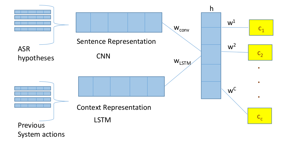
Figure 1: Combination of sentence and context representations for the joint optimisation. In the first step, the binary classifiers $c_{i}$ are predicting the presence or absence of slots. In the second step, they are predicting the presence or absence of the values for a given slot.

All the weights in the neural network are optimised jointly. The benefits of joint inference have been published in the past for different NLP tasks Singh et al. (2013); Liu and Lane (2016). The main advantage of joint-inference is that parameters are shared between predictors, thus weights can be adjusted based on their mutual influence. For instance, the most frequent slots might influence infrequent slots.

4 Risk Minimisation (RM)

We use the unsupervised approach proposed in Balasubramanian et al. (2011) for risk minimisation (RM). We assume a binary classifier that associates a score $f_{\mathbf{W}_{0}}(\mathbf{h})$ to the first class 0 for the hidden unit $\mathbf{h}=(h_{1},\cdots,h_{n})$ of dimension $n$:

$$f_{W_{0}}(\mathbf{h})=\sum_{i}^{n}w_{i}h_{i}$$

where the parameter $w_{i}\in{\rm I\!R}$ represents the weight of the feature indexed by $i$ for class 0.

The objective of training is to minimize the classifier risk:

$$R(\mathbf{W})=E_{p(\mathbf{h},Y)}[\mathcal{L}(Y,f_{\mathbf{W}}(\mathbf{h}))]$$ (3)

where $Y$ is the true label and $\mathcal{L}(Y,f_{\mathbf{W}}(\mathbf{h}))$ is the loss function. The risk is derived as follows:

$$R(\mathbf{W})=\sum_{y\in\{0,1\}}P(y)\int_{-\infty}^{+\infty}P(f_{\mathbf{W}}(\mathbf{h})=\alpha|y)\mathcal{L}(y,\alpha)d\alpha$$ (4)

We use the following hinge loss:

$$\mathcal{L}(y,\alpha)=\left(1+\alpha_{1-y}-\alpha_{y}\right)_{+}$$ (5)

where $(z)_{+}=\max(0,z)$, and $\alpha_{y}=f_{\mathbf{W}_{y}}(\mathbf{h})$ is the linear score for the correct class $y$. Similarly, $\alpha_{1-y}=f_{\mathbf{W}_{1-y}}(\mathbf{h})$ is the linear score for the wrong class.

Given $y$ and $\alpha$, the loss value in the integral (Equation 4) can be computed easily. Two terms remain: $P(y)$ and $P(f_{\mathbf{W}}(\mathbf{h})=\alpha|y)$. The former is the class marginal and is assumed to be known. The latter is the class-conditional distribution of the linear scores, which is assumed to be normally distributed. This implies that $P(f_{\mathbf{W}}(\mathbf{h}))$ is distributed as a mixture of two Gaussians (GMM):

$$P(f_{\mathbf{W}}(\mathbf{h}))=\sum_{y\in\{0,1\}}P(y)\mathcal{N}(f_{\mathbf{W}}(\mathbf{h});\mu_{y},\sigma_{y})$$

where $\mathcal{N}(z;\mu,\sigma)$ is the normal probability density function. The parameters $(\mu_{0},\sigma_{0},\mu_{1},\sigma_{1})$ can be estimated from an unlabeled corpus $\mathcal{U}$ using a standard Expectation-Maximization (EM) algorithm for GMM training. Once these parameters are known, it is possible to compute the integral in Eq. 4 and thus an estimate $\hat{R}(\mathbf{W})$ of the risk without relying on any labeled corpus. In  Balasubramanian et al. (2011), it has been proven that: (i) the Gaussian parameters estimated with EM converge towards their true values, (ii) $\hat{R}(\mathbf{W})$ converges towards the true risk $R(\mathbf{W})$ and (iii) the estimated optimum converges towards the true optimal parameters, when the size of the unlabeled corpus increases infinitely. This is still true even when the class priors $P(y)$ are unknown.

The unsupervised algorithm is as follows:

Unsupervised tuning for the binary classifier $c$, where $c=1,...,C$

1:input: $\mathbf{h}$ the top hidden layer and the weights $\mathbf{W}^{c}$, as trained by the deep learning decoder (Section 3).

2:output: The tuned weights $\hat{\mathbf{W}}^{c}$

3:repeat

4:     for every index $i$ in $\mathbf{h}$ do ,

5:         Change the weights $\mathbf{W}^{c}_{i}=\mathbf{W}^{c}_{i}+\delta$,

6:         Estimate the Gaussian parameters using EM

7:         Compute the risk (Eq. 4) on the unlabeled corpus $\mathcal{U}$ (i.e. the evaluation set).

8:         Compute the gradient using finite differences

9:         Update the weights accordingly $\hat{\mathbf{W}}^{c}_{i}=\mathbf{W}^{c}_{i}$

10:     end for

11:until convergence

5 Experiments

The supervised and unsupervised models are evaluated on DSTC3 Henderson et al. (2014) using the macro F-Measure. We compare then three distinct models, (i) independent neural models for every binary classifier; (ii) neural models optimised jointly and (iii) further tuning of the weights through RM.

Dataset

As displayed in Table 1 in DSTC3 new slots were introduced relative to DSTC2. The training set contains only a few examples of these slots while the test set contains a large number of them. Interestingly, frequent values per slots in the trainset such as area=north, are absolutely absent in the testset. In DSTC3 the dialogues are related to restaurants, pubs and coffee shops. The new slots are: childrenallowed, hastv, hasinternet and near. Known slots, such as food, can have zero-shot values as shown in Table 2. The corpus contains $3246$ dialogues, $25610$ turns in the trainset and $2264$ dialogues, $18715$ turns in the testset.

Hyperparameters and Training

The neural models were implemented in Theano Bastien et al. (2012). We used filter windows of 3, 4, and 5 with 100 feature maps each for the CNN. A dropout rate of $0.5$ and a batch size of 50 was employed. Training is done through stochastic gradient descent over shuffled mini-batches with the Adadelta update rule. GloVE word vectors were used Pennington et al. (2014) to intialise the models with a dimension $n=100$. For the context representation, we use a window of the 4 previous system acts. The risk minimisation gradient descent runs during 2000 iterations for each binary classifier and the class priors $P(y)$ were set to $0.01$ and $0.99\%$ for the positive and negative classes respectively.

Slot	$\#$Train	$\#$Test
hastv	1	239
childrenallowed	2	119
near	3	74
hasinternet	4	215
area	3149	5384
food	5744	7809

Table 1: Frequency of slots in DSTC3.

Slot	Value	$\#$Train	$\#$Test
near	trinity college	0	5
food	american	0	90
food	chinese takeaway	0	87
area	romsey	0	127
area	girton	0	118

Table 2: Some zero-shot values per slots in DSTC3.

The Gaussianity Assumption

As explained in Section 4, the risk minimisation tuning assumes the class-conditional linear scores are distributed normally. We verified this assumption empirically on our unlabeled corpus $\mathcal{U}$ (i.e. DSTC3 testset) and we found that for the slots: childrenallowed, hastv and hasinternet this assumption holds. However, the distribution for near has a negative skew. When verifying the values per slot, this assumption does not hold for area. Therefore, we can not guarantee this method will work correctly for area values on this evaluation set.

Deep Learning Independent Models
Slot	F-Measure
childrenallowed	$49.84$%
hastv	$49.68$%
hasinternet	$49.72$%
near	$49.90$%
Deep Learning Joint Optimisation
childrenallowed	$58.76$%
hastv	$59.16$%
hasinternet	$58.77$%
near	$56.65$%
Risk Minimisation Tuning
childrenallowed	$\mathbf{61.64}$%
hastv	$\mathbf{61.35}$%
hasinternet	$\mathbf{60.87}$%
near	$\mathbf{58.60}$%

Table 3: Results for learning rare slots on DSTC3 evaluation set.

Deep Learning Independent Models
Slot	Value	F-Measure
near	trinity college	$49.99$%
food	american	$49.88$%
	chinese take away	$49.88$%
area	romsey	$49.83$%
	girton	$49.84$%
Deep Learning Joint Optimisation
near	trinity college	$61.25$%
food	american	$59.93$%
	chinese take away	$61.02$%
area	romsey	$\mathbf{51.30}$%
	girton	$\mathbf{55.19}$%
Risk Minimisation Tuning
near	trinity college	$\mathbf{62.08}$%
food	american	$\mathbf{62.52}$%
	chinese take away	$\mathbf{63.79}$%
area	romsey	$48.76$%
	girton	$51.45$%

Table 4: Results for learning zero shot slot-value pairs on DSTC3 evaluation set.

6 Results

Tables 3 and 4 display the performance of the models that predict slots and values respectively. The low F-Measure in the independent models shown their inability to predict positive examples. The models improve significantly the precision and F-Measure after the joint-optimisation. Applying RM tuning results in the best F-Measure for all the rare slots (Table 3) and for the values of the slots food and near (Table 4). For area, the joint optimisation improves the F-Measure but the improvement is lower than for other slots. The performance is being affected by its low cardinality (i.e. $20$), the high variability of new places and the fact that frequent values such as north and east, are completely absent in the test set. As suspected, the RM tuning degraded the precision and F-Measure because the Gaussianity assumption does not hold for area. However, RM will work well in larger evaluation sets because the Gaussian assumption will hold when the unlabeled corpus tends to infinite (please refer to  Balasubramanian et al. (2011) for the theoretical proofs).

7 Conclusion

We presented here two novel methods for zero-shot learning in a deep semantic decoder. First, features and weights were learned through a joint optimisation within a deep learning architecture. Second, the weights were further tuned through risk minimisation. We have shown that the joint optimisation significantly improves the neural models for nearly zero-shot slots. We have also shown that under the Gaussianity assumption, the RM tuning is a promising method for further tuning the weights of zero-shot data in an unsupervised way.

References

- Balasubramanian et al. (2011) Krishnakumar Balasubramanian, Pinar Donmez, and Guy Lebanon. 2011. Unsupervised supervised learning II: Margin-based classification without labels. Journal of Machine Learning Research 12:3119–3145.
- Bastien et al. (2012) Frédéric Bastien, Pascal Lamblin, Razvan Pascanu, James Bergstra, Ian Goodfellow, Arnaud Bergeron, Nicolas Bouchard, and Yoshua Bengio. 2012. Theano: new features and speed improvements. nips workshop on deep learning and unsupervised feature learning .
- Daumé III (2009) Hal Daumé III. 2009. Frustratingly easy domain adaptation. arXiv preprint arXiv:0907.1815 .
- Ferreira et al. (2015) Emmanuel Ferreira, Bassam Jabaian, and Fabrice Lefevre. 2015. Online adaptative zero-shot learning spoken language understanding using word-embedding. In Acoustics, Speech and Signal Processing (ICASSP), 2015 IEEE International Conference on. IEEE, pages 5321–5325.
- Gardent and Rojas Barahona (2013) Claire Gardent and Lina Maria Rojas Barahona. 2013. Using Paraphrases and Lexical Semantics to Improve the Accuracy and the Robustness of Supervised Models in Situated Dialogue Systems. In Conference on Empirical Methods in Natural Language Processing. SIGDAT, the Association for Computational Linguistics special interest group on linguistic data and corpus-based approaches to NLP, Seattle, United States, pages 808–813. https://hal.inria.fr/hal-00905405.
- Glorot et al. (2011) Xavier Glorot, Antoine Bordes, and Yoshua Bengio. 2011. Domain adaptation for large-scale sentiment classification: A deep learning approach. In Proceedings of the 28th international conference on machine learning (ICML-11). pages 513–520.
- Henderson et al. (2014) Matthew Henderson, Blaise Thomson, and Jason Williams. 2014. The third dialog state tracking challenge. In Proceedings IEEE Spoken Language Technology Workshop (SLT). IEEE â Institute of Electrical and Electronics Engineers.
- Liu and Lane (2016) Bing Liu and Ian Lane. 2016. Joint online spoken language understanding and language modeling with recurrent neural networks. arXiv preprint arXiv:1609.01462 .
- Mesnil et al. (2013) Grégoire Mesnil, Xiaodong He, Li Deng, and Yoshua Bengio. 2013. Investigation of recurrent-neural-network architectures and learning methods for spoken language understanding. In Interspeech. pages 3771–3775.
- Mikolov et al. (2013) Tomas Mikolov, Kai Chen, Greg Corrado, and Jeffrey Dean. 2013. Efficient estimation of word representations in vector space. arXiv preprint arXiv:1301.3781 .
- Mrksic et al. (2017) Nikola Mrksic, Ivan Vulic, Diarmuid Ó Séaghdha, Ira Leviant, Roi Reichart, Milica Gasic, Anna Korhonen, and Steve J. Young. 2017. Semantic specialization of distributional word vector spaces using monolingual and cross-lingual constraints. Transactions of the Association for Computational Linguistics 5:309–324. https://www.transacl.org/ojs/index.php/tacl/article/view/1171.
- Pappu and Rudnicky (2013) Aasish Pappu and Alexander I Rudnicky. 2013. Predicting tasks in goal-oriented spoken dialog systems using semantic knowledge bases. In SIGDIAL Conference. pages 242–250.
- Pennington et al. (2014) Jeffrey Pennington, Richard Socher, and Christopher D. Manning. 2014. Glove: Global vectors for word representation. In Empirical Methods in Natural Language Processing (EMNLP). pages 1532–1543. http://www.aclweb.org/anthology/D14-1162.
- Rojas Barahona et al. (2016) Lina M. Rojas Barahona, Milica Gasic, Nikola Mrkšić, Pei-Hao Su, Stefan Ultes, Tsung-Hsien Wen, and Steve Young. 2016. Exploiting sentence and context representations in deep neural models for spoken language understanding. In Proceedings of COLING 2016, the 26th International Conference on Computational Linguistics: Technical Papers. The COLING 2016 Organizing Committee, Osaka, Japan, pages 258–267. http://aclweb.org/anthology/C16-1025.
- Rojas Barahona and Cerisara (2015) Lina Maria Rojas Barahona and Christophe Cerisara. 2015. Weakly supervised discriminative training of linear models for Natural Language Processing. In 3rd International Conference on Statistical Language and Speech Processing (SLSP). Budapest, Hungary. https://hal.archives-ouvertes.fr/hal-01184849.
- Singh et al. (2013) Sameer Singh, Sebastian Riedel, Brian Martin, Jiaping Zheng, and Andrew McCallum. 2013. Joint inference of entities, relations, and coreference. In Proceedings of the 2013 Workshop on Automated Knowledge Base Construction. ACM, New York, NY, USA, AKBC ’13, pages 1–6. https://doi.org/10.1145/2509558.2509559.
- Tur et al. (2012) Gokhan Tur, Minwoo Jeong, Ye-Yi Wang, Dilek Hakkani-Tür, and Larry Heck. 2012. Exploiting the semantic web for unsupervised natural language semantic parsing .
- Zhou et al. (2016) Guangyou Zhou, Zhiwen Xie, Jimmy Xiangji Huang, and Tingting He. 2016. Bi-transferring deep neural networks for domain adaptation. In ACL (1).
- Zhu et al. (2014) Su Zhu, Lu Chen, Kai Sun, Da Zheng, and Kai Yu. 2014. Semantic parser enhancement for dialogue domain extension with little data. In Spoken Language Technology Workshop (SLT), 2014 IEEE. IEEE, pages 336–341.