Stabilization with a Specified External Gain for Linear MIMO Systems and Its Applications to Control of Networked Systems

Abstract

This paper studies a stabilization problem for linear MIMO systems subject to external perturbation that further requires the closed-loop system render a specified gain from the external perturbation to the output. The problem arises from control of networked systems, in particular, robust output synchronization of heterogeneous linear MIMO multi-agent systems via output feedback/communication. We propose a new approach that converts a class of MIMO systems into a normal form via repeated singular value decomposition and prove that a stabilization controller with a specified external gain can be explicitly constructed for the normal form. Two scenarios with static state feedback and dynamic output feedback are investigated. By integrating the reference model and internal model techniques, the robust output synchronization problem for MIMO multi-agent systems is converted into a stabilization problem with a specified external gain and solved by the developed approach.

, , ,

1 Introduction

Stabilization for linear MIMO systems is a well developed and widely used technique in modern control theory. The main focus of this paper is study a stabilization problem for linear MIMO systems subject to external perturbation that further requires the closed-loop system render a specified gain from the external perturbation to the output. The tool to characterize the gain from the external perturbation to the output is the so-called input-to-output stability (IOS) gain with the external perturbation regarded as an input to the closed-loop system [1, 2].

It is known that when a linear system is stabilizable, a feedback controller that renders the asymptotic stability for the system free of external perturbation also makes the closed-loop system IOS when external perturbation is taken into consideration. The IOS gain is determined by the closed-loop system structure. However, it remains a challenging task when an input-to-output stabilization further requires an arbitrarily specified external gain. That requires an input-to-output stabilization controller to further achieve an arbitrarily specified external gain. Such a stabilization is interesting by itself when one is interested in managing the external influence to system output through the stabilization controller design. Also, the problem is well motivated from studying networked systems.

A relevant research topic in the literature is $H_{\infty}$ and $H_{2}$ (sub)optimal control. For example, Sontag discussed the close relation between input-to-state/output formulation and $H_{\infty}$ and $H_{2}$ (sub)optimal control in [3]. It is known that the solution of $H_{\infty}$ and $H_{2}$ control relies on the solution of Riccati equations for a linear system [4] and Hamilton-Jacobi-Isaacs partial differential equations for nonlinear systems [5, 6, 7, 8]. What differs from input-to-output stabilization here is that the $H_{\infty}$ or $H_{2}$ gain through admissible state feedback and output feedback control is greater or equal than a minimum which depends on the system structure and the solutions to Riccati equations. In other words, the impact of a perturbation in terms of $H_{\infty}$ or $H_{2}$ gain can be optimized/minimized by feedback control, but not made arbitrarily small. However, the problem studied in this paper requires an arbitrarily specified external gain through feedback controller design.

One sufficient condition for the solvability of $H_{\infty}$ or $H_{2}$ control is that the linear system is stabilizable and detectable and the solutions to the corresponding Riccati equations exist. The conditions needed for the stronger requirement on arbitrarily specified external gain are studied in paper. In particular, with some additional conditions, linear MIMO systems can be transformed to a so-called normal form for which the problem can be solved. It is noted that the same problem has been solved for nonlinear minimum-phase systems in the previous paper [9] using the backstepping technique and the improved small gain theorem. But the systems in [9] are SISO and in the so-called lower triangular form. Therefore, the result cannot be applied in the present MIMO and non-lower-triangular systems.

An important motivation or application of the proposed technique of stabilization with a specified external gain is the robust output synchronization problem for heterogeneous multi-agent systems through output feedback and output communication. Heterogeneity among agents is commonly encountered in real-world applications such as vehicle platoons in [10] and power systems in [11] where the dynamics of subsystems are not uniform. Synchronization of multi-agent systems aims to achieve the agreement on agents’ outputs via local communication among agents despite the heterogeneity. For homogeneous multi-agent systems, the synchronization pattern is naturally embedded in the homogeneous part of agents’ dynamics, but it is not explicit for heterogeneous systems. In [12], a necessary condition for synchronization of heterogeneous multi-agent systems called internal model principle has been given as that there must exist a homogeneous kernel for each agent that embraces the synchronization pattern. The homogeneous kernel is either embedded in the original dynamics or explicitly constructed through the controller design according to the task.

More specifically, as exposed in many works, e.g., [12, 13, 14, 15, 16], the synchronization controller of heterogeneous multi-agent systems can be explicitly constructed in a two-step manner. The first step is the consensus of reference models that are constructed to be homogeneous for each agent and embed the homogeneous kernel. The second step is the regulation of each individual agent’s output to the output of its own reference model. In particular, when agent dynamics contain no uncertainties, the regulation can be achieved by the feedforward compensation control. This method was utilized for the synchronization of linear systems in [12] and nonlinear systems in [17]. However, the exact feedforward compensation becomes impossible if agent dynamics have uncertainties (see detailed discussion in [15]). In this case, researchers appeal to robust output regulation theory to handle uncertainties. It relies on a class of dynamic observers called internal model (in the context of robust output regulation theory) whose dynamics do not depend on the uncertainties but asymptotically generate the steady-state solution for states and/or control input. With the internal model, the regulation problem can be converted into a stabilization problem for which a feedback controller can be designed. This method has been used for the robust output synchronization for linear systems in [18] and nonlinear systems in [14, 16].

More specifically, synchronization controllers can be classified to rely on the state or output communication. For state communication, each agent is allowed to transmit its internal states to its neighbors, while for output communication, it becomes slightly more restrictive and only the output information is allowed to transmit. The freedom to choose what internal information to transmit over the network makes synchronization on state communication less complicated than that on output communication. Consequently, the aforementioned two actions, namely consensus for reference models and regulation of each agent to its reference, can be completely separated for state communication, which simplifies the controller design procedure [ChenXi2016]. For the output communication case, the work in [16] shows that these two actions are mutually perturbed by each other (hence further called perturbed consensus and perturbed regulation). In particular, the consensus action is perturbed by the regulation error and the regulation action is disturbed by the disagreement in consensus. The output synchronization framework via output communication developed in [16] suggests that synchronization is achieved if both perturbed consensus and perturbed regulation are solved as well as a small gain condition is satisfied.

The robust output synchronization of heterogeneous linear MIMO multi-agent systems via output communication is yet to be investigated and is the focus of the second part of this paper. In particular, we need to propose a modified internal model and show that the robust output synchronization problem of MIMO multi-agent systems can also be converted into perturbed consensus and perturbed regulation problems. Moreover, the perturbed regulation problem corresponds to the stabilization problem which can be solved using techniques developed in the first part of the paper

The rest of this paper is structured as follows. In Section 2, we will first introduce the problem of stabilization with a specified external gain and its motivation. The main results on stabilization with a specified external gain are given in Section 3. In particular, we propose a state feedback controller for the MIMO systems in the normal form as well as a dynamic output feedback controller for systems of a special structure. In Section 4, we formulate the robust output synchronization problem for linear heterogeneous MIMO multi-agent systems and introduce the framework that converts the problem into a standard perturbed consensus problem and a perturbed regulation problem. Moreover, with the aid of modified internal model design, we show that the perturbed regulation problem is equivalent to the stabilization problem with a specified gain as studied in Section 2. The numerical simulation is conducted in Section 5 and the paper is concluded in Section 6.

2 Problem Formulation and Motivation

We consider a class of linear MIMO control systems typically represented by the following equations

$$\dot{x} = Ax+Bu+R\zeta$$

$$y = Cx,$$ (1)

where $x\in\mathbb{R}^{n}$ is the state, $u\in\mathbb{R}^{m}$ the input, $y\in\mathbb{R}^{p}$ the output, and $\zeta\in\mathbb{R}^{\ell}$ external perturbation. The matrices $A\in\mathbb{R}^{n\times n}$, $B\in\mathbb{R}^{n\times m}$, $R\in\mathbb{R}^{n\times\ell}$ and $C\in\mathbb{R}^{p\times n}$ have compatible dimensions. The external perturbation $\zeta$ may represent external signals or influence of other subsystem to the system (1) in an interconnected setting.

A general linear controller takes a static form

$$u=Kx$$ (2)

or a dynamic form

$$u = K\chi$$

$$\dot{\chi} = A\chi+L(y-C\chi)+Bu+R\zeta$$ (3)

that induces a closed-loop system

$$\dot{x}_{c} = A_{c}x_{c}+R_{c}\zeta$$

$$y = C_{c}x_{c}$$ (4)

for $x_{c}=x$ or $x_{c}=\mbox{col}(x,\chi)$, respectively.

Without the external perturbation $\zeta$, the stabilization controller design for a linear system is well known in the literature. Moreover, for any stabilization controller that ensures a Hurwitz $A_{c}$, the basic property of a linear system implies that the closed-loop system (4) is automatically bounded input bounded output (BIBO) or input-to-output stable (IOS), with $\zeta$ as the input and $y$ the output. Also, the gain from $\zeta$ to $y$ can be explicitly computed. However, it remains a difficult task to design a stabilization controller such that the closed-loop system (4) has an arbitrarily specified gain from $\zeta$ to $y$.

More specifically, we will use a quadratic function to characterize the relationship between the input and output for the linear closed-loop system (4).

Definition 2.1.

The linear MIMO system (4) with a Hurwitz matrix $A_{c}$ is said to admit a quadratic IOS-Lyapunov function $V(x_{c})=x_{c}^{\mbox{\tiny{T}}}Px_{c}$ with $P=P^{\mbox{\tiny{T}}}>0$ if there exist positive constants $\alpha$ and $\beta$ such that

$$\dot{V}(x)\leq-\alpha\|y\|^{2}+\beta\|\zeta\|^{2}.$$ (5)

In particular, $\beta/\alpha$ is called an IOS gain.  

Remark 2.1.

The gain between $\zeta$ to $y$ is called an IOS gain because the external perturbation $\zeta$ is regarded as an input to the closed-loop system (4). To avoid any confusion between $\zeta$ and the actual input $u$ for the open-loop system (1), we call the gain an external gain throughout the paper.  

With the aforementioned setting, the main objective of this paper is rigorously formulated in the following problem.

The problem of stabilization with a specified external gain $\gamma$ ($\gamma$-stabilization) for the system (1) aims, for an arbitrarily specified $\gamma>0$, to find a controller (2) or (3) such that the system (4) has a Hurwitz matrix $A_{c}$ and an external gain $\gamma$.

The $\gamma$-stabilization problem has an independent interest when one is interested in managing the influence of an external signal to system output through the stabilization controller design. Also, the problem is well motivated from studying networked systems. One simple motivating example is given below. A complete application of $\gamma$-stabilization can be found in Section 4 in effectively solving the robust output synchronization problem for heterogeneous MIMO multi-agent systems.

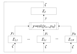
Figure 1: Interconnection of a network of MIMO control systems $\Sigma_{1,i}$, $i=1,\cdots,N$ and an MIMO system $\Sigma_{2}$.

Example 2.1.

Consider the interconnection of two subsystems illustrated in Fig. 1. The first subsystem $\Sigma_{1}=(\Sigma_{1,i},\cdots,\Sigma_{1,N})$ is a network of $N$ linear MIMO control systems described by (1), that is,

$$\Sigma_{1,i}:\begin{array}[]{c}\dot{x}_{i}=A_{i}x_{i}+B_{i}u_{i}+R_{i}\zeta,\\ y_{i}=C_{i}x_{i},\end{array},\;i=1,\cdots,N$$ (6)

where $x_{i}\in\mathbb{R}^{n_{i}}$, $u_{i}\in\mathbb{R}^{m_{i}}$ and $y_{i}\in\mathbb{R}^{p_{i}}$ are the state, input and output, respectively and $y=\mbox{col}(y_{1},\cdots,y_{N})$ is the composite output of $\Sigma_{1}$. The second subsystem $\Sigma_{2}$ is given by

$$\Sigma_{2}:\begin{array}[]{c}\dot{\tau}=A_{\tau}\tau+R_{\tau}y,\\ \zeta=C_{\tau}\tau,\end{array}$$ (7)

where $\tau\in\mathbb{R}^{n_{\tau}}$ is the state and $\zeta\in\mathbb{R}^{\ell}$ the output. The subsystems $\Sigma_{1}$ and $\Sigma_{2}$ are coupled through their respective outputs $\zeta$ and $y$. Suppose $\Sigma_{2}$ admits a quadratic IOS-Lyapunov function and an external gain $\gamma_{\zeta}$. Then, the $\gamma$-stabilization for each $\Sigma_{1,i}$ with the external gain $\gamma<1/(N\gamma_{\zeta})$ guarantees stability of the overall system by using Proposition 2.1 stated below.

For $N=1$, it is a typical interconnection of two subsystems studied in many references such as [19, 20]. The present scenario with $N>1$ derives from the robust output synchronization studied in, e.g., [16]. The two interconnected subsystems $\Sigma_{1}$ and $\Sigma_{2}$ correspond to the dynamics for perturbed consensus and perturbed regulation problems to be elaborated in Section 4.  

The following proposition shows how $\gamma$-stabilization for each $\Sigma_{1,i}$ guarantees the stability of the overall system in Example 2.1.

Proposition 2.1.

For the control system composed of (6) and (7), if $\Sigma_{2}$ admits a quadratic IOS-Lyapunov function and an external gain $\gamma_{\zeta}$ and the $\gamma$-stabilization problem for each $\Sigma_{1,i}$ with the external gain $\gamma<1/(N\gamma_{\zeta})$ is solved by a linear controller. Then, the overall closed-loop linear system is stable.  

Proof: Let the quadratic IOS-Lyapunov function for $\Sigma_{2}$ be $V_{\tau}(\tau)$ that satisfies

$$\dot{V}_{\tau}(\tau)\leq-\alpha_{\zeta}\|\zeta\|^{2}+\beta_{\zeta}\|y\|^{2}$$ (8)

for some $\alpha_{\zeta},\beta_{\zeta}>0$ satisfying $\gamma_{\zeta}=\beta_{\zeta}/\alpha_{\zeta}$. Let the state of the system composed of $\Sigma_{1,i}$ and its $\gamma$-stabilization controller be $x_{c,i}$. Then, solvability of the $\gamma$-stabilization problem for $\Sigma_{1,i}$ means the existence of a quadratic IOS-Lyapunov function $V_{i}(x_{c,i})$ that satisfies

$$\dot{V}_{i}(x_{c,i})\leq-\alpha_{i}\|y_{i}\|^{2}+\beta_{i}\|\zeta\|^{2},\;i=1,\cdots,N$$ (9)

for some $\alpha_{i},\beta_{i}>0$ satisfying $\gamma=\beta_{i}/\alpha_{i}$.

Let $x_{c}=\mbox{col}(x_{c,1},\cdots,x_{c,N})$ and

$$V(\tau,x_{c})={V}_{\tau}(\tau)/\beta_{\zeta}+\epsilon\sum_{i=1}^{N}V_{i}(x_{c,i})/\alpha_{i},\;\epsilon>0$$

whose derivative along the trajectory of the overall closed-loop system is

$$\dot{V}(\tau,x_{c})\leq-\alpha_{\zeta}/\beta_{\zeta}\|\zeta\|^{2}+\|y\|^{2}-\epsilon\sum_{i=1}^{N}\|y_{i}\|^{2}+\epsilon\sum_{i=1}^{N}\beta_{i}/\alpha_{i}\|\zeta\|^{2}$$

$$\leq-1/\gamma_{\zeta}\|\zeta\|^{2}+\|y\|^{2}-\epsilon\|y\|^{2}+\epsilon N\gamma\|\zeta\|^{2}$$

$$\leq-(1/\gamma_{\zeta}-\epsilon N\gamma)\|\zeta\|^{2}-(\epsilon-1)\|y\|^{2}.$$

As $\gamma<1/(N\gamma_{\zeta})$, we can pick

$$\frac{1}{N\gamma\gamma_{\zeta}}>\epsilon>1,$$

that is,

$$1/\gamma_{\zeta}-\epsilon N\gamma>0,\;\epsilon-1>0.$$

Applying Lasalle-Yoshizawa Theorem ([21]) leads to the state of the closed-loop has the following asymptotical property

$$\lim_{t\rightarrow\infty}\zeta(t)=0,\;\lim_{t\rightarrow\infty}y(t)=0,$$ (10)

which further implies

$$\lim_{t\rightarrow\infty}\tau(t)=0,\;\lim_{t\rightarrow\infty}x_{c}(t)=0.$$ (11)

The proof is thus completed.  

3 Main Results: $\gamma$-Stabilization

The first main result is to explicitly find a state feedback controller (2) to solve the $\gamma$-stabilization problem for the system (1). For this purpose, we introduce a state transformation based on the singular value decomposition of the input matrix that puts the system into a class of normal form.

3.1 A Normal Form

Let us recursively define a sequence of matrix pairs $(\Phi_{j},\Gamma_{j})$, $j=0,1,\cdots$ in the following algorithm. In the algorithm, denote the rank of $\Gamma_{j}$ by $r_{j}$, i.e., $\mbox{rank}(\Gamma_{j})=r_{j}.$ For convenience of notation, let $r_{-1}=m$.

• Let $j=0$ and set the initial values

  $$\Phi_{0}=A,\;\Gamma_{0}=B.$$

• If $\Gamma_{j}$ has a full row rank or $\Gamma_{j}=0$, exit.

• One has

  $$\Phi_{j}\in\mathbb{R}^{(n-\Sigma_{k=0}^{j-1}r_{k})\times(n-\Sigma_{k=0}^{j-1}r_{k})},\;\Gamma_{j}\in\mathbb{R}^{(n-\Sigma_{k=0}^{j-1}r_{k})\times r_{j-1}}$$

  and the singular value decomposition (SVD) of $\Gamma_{j}$ is

  $$\Gamma_{j}=U_{j+1}\left[\begin{array}[]{cc}\Sigma_{j}&0\\ 0&0\end{array}\right]H_{j+1}^{\mbox{\tiny{T}}},$$ (12)

  where $\Sigma_{j}\in\mathbb{R}^{r_{j}\times r_{j}}$ is a diagonal matrix bearing all non-zero singular values on the diagonal entries and $U_{j+1}\in\mathbb{R}^{(n-\Sigma_{k=0}^{j-1}r_{k})\times(n-\Sigma_{k=0}^{j-1}r_{k})}$ and $H_{j+1}\in\mathbb{R}^{r_{j-1}\times r_{j-1}}$ are unitary matrices.

  Since $\Gamma_{j}$ does not have a full row rank and $\Gamma_{j}\neq 0$ (otherwise exit at step (ii)), one has $n-\Sigma_{k=0}^{j-1}r_{k}>r_{j}>0$ and hence the following decomposition

  $$U_{j+1}=\left[\begin{array}[]{cc}\tilde{U}_{j+1}&\bar{U}_{j+1}\end{array}\right],\;\tilde{U}_{j+1}\in\mathbb{R}^{(n-\Sigma_{k=0}^{j-1}r_{k})\times r_{j}},\;\bar{U}_{j+1}\in\mathbb{R}^{(n-\Sigma_{k=0}^{j-1}r_{k})\times(n-\Sigma_{k=0}^{j}r_{k})}.$$

  Calculate

  $$\Phi_{j+1}=\bar{U}_{j+1}^{\mbox{\tiny{T}}}\Phi_{j}\bar{U}_{j+1}\in\mathbb{R}^{(n-\Sigma_{k=0}^{j}r_{k})\times(n-\Sigma_{k=0}^{j}r_{k})}$$

  $$\Gamma_{j+1}=\bar{U}_{j+1}^{\mbox{\tiny{T}}}\Phi_{j}\tilde{U}_{j+1}\in\mathbb{R}^{(n-\Sigma_{k=0}^{j}r_{k})\times r_{j}}.$$ (14)

• Let $j=j+1$ and go to step (ii).

Then, the next lemma shows a useful result from the above algorithm under a controllability assumption. The proof is given in the Appendix.

Assumption 3.1.

The pair of matrices $(A,B)$ is controllable.  

Lemma 3.1.

Consider the linear system (1) satisfying Assumption 3.1. Then, there exists a finite number $l$ such that $\Gamma_{l}$ defined in the algorithm has a full row rank. Moreover, the pair $(\Phi_{j},\Gamma_{j})$ is controllable for $0\leq j\leq l$.  

Throughout the paper, we call $l$ in Lemma 3.1 the number of SVD steps. With the finite number $l$, we define the orthogonal matrix

$$T=\left[\begin{array}[]{c}T_{1}\\ T_{2}\\ \vdots\\ T_{l}\\ T_{l+1}\end{array}\right]:=\left[\begin{array}[]{c}\bar{U}_{l}^{\mbox{\tiny{T}}}\cdots\bar{U}_{1}^{\mbox{\tiny{T}}}\\ \tilde{U}_{l}^{\mbox{\tiny{T}}}\bar{U}_{l-1}^{\mbox{\tiny{T}}}\cdots\bar{U}_{1}^{\mbox{\tiny{T}}}\\ \vdots\\ \tilde{U}_{2}^{\mbox{\tiny{T}}}\bar{U}_{1}^{\mbox{\tiny{T}}}\\ \tilde{U}_{1}^{\mbox{\tiny{T}}}\end{array}\right]\in\mathbb{R}^{n\times n},\;\begin{array}[]{c}T_{1}\in\mathbb{R}^{(n-\Sigma_{k=0}^{l-1}r_{k})\times n}\\ T_{2}\in\mathbb{R}^{r_{l-1}\times n}\\ \vdots\\ T_{l}\in\mathbb{R}^{r_{1}\times n}\\ T_{l+1}\in\mathbb{R}^{r_{o}\times n}\end{array}.$$ (15)

where $T\in\mathbb{R}^{n\times n}$. Accordingly, we introduce the coordinate transformation

$$\xi:=\left[\begin{array}[]{ccc}\xi_{1}^{\mbox{\tiny{T}}}&\cdots&\xi_{l+1}^{\mbox{\tiny{T}}}\end{array}\right]^{\mbox{\tiny{T}}}=Tx$$ (16)

with the dimension of $\xi_{j}$ compatible with $T_{j}$.

We need one more assumption to obtain the input-to-output stabilization normal form for the system (1).

Assumption 3.2.

The matrices $(A,B,C)$ satisfy $CA^{j-1}B=0$ for $j=1,\cdots,l$.  

Lemma 3.2.

Consider linear MIMO system (1) under Assumptions 3.1 and 3.2. Then, $CT_{j}^{\mbox{\tiny{T}}}=0$ for $j=2,\cdots,l+1$ and hence

$$y=Cx=C_{\xi}\xi_{1}.$$ (17)

for $C_{\xi}=CT_{1}^{\mbox{\tiny{T}}}$.  

Proof: The proof is given in Appendix.  

Now, we can define the following matrices recursively,

$$A_{1}=\Phi_{l},\;B_{1}=\Gamma_{l},\;R_{1}=T_{1}R,$$

and, for $j=2,\cdots,l+1$,

$$\begin{split}A_{j}&=\tilde{U}_{l+2-j}^{\mbox{\tiny{T}}}\Phi_{l+1-j}\tilde{U}_{l+2-j}\\ B_{j}&=\left[\begin{array}[]{cc}\Sigma_{l+1-j}&0\end{array}\right]H_{l+2-j}^{\mbox{\tiny{T}}}\\ R_{j}&=T_{j}R.\end{split}$$

Also, define

$$D_{j,k}=T_{j}AT_{k}^{\mbox{\tiny{T}}},\;k=1,\cdots,j-1,\;j=1,\cdots,l+1.$$

Then, the system (1) with the state transformation (16) under Assumptions 3.1 and 3.2 can be converted to the following form, with $u=\xi_{l+2}$,

$$\dot{\xi}_{j} = A_{j}\xi_{j}+B_{j}\xi_{j+1}+\Sigma_{k=1}^{j-1}D_{j,k}\xi_{k}+R_{j}\zeta,\;j=1,\cdots,l+1$$

$$y = C_{\xi}\xi_{1}.$$ (18)

Remark 3.1.

From the above development, Lemma 3.1 shows that $B_{1}$ is of full row rank. Since $\Sigma_{0},\cdots,\Sigma_{l-1}$ and $H_{1},\cdots,H_{l}$ are nonsingular, $B_{2},\cdots,B_{l+1}$ are of full row rank. In this sense, the system (18) has a block lower-triangular normal form. It is easy to see that the solution to the $\gamma$-stabilization problem for the system (18) implies that of (1).  

3.2 State Feedback Control

In this subsection, we will show how a static state controller can be designed for the $\gamma$-stabilization problem of the system (18) and hence (1).

Theorem 3.1.

(State Feedback) Consider the linear MIMO system (1) under Assumptions 3.1 and 3.2. Then, there exists a matrix $K$ such that the controller

$$u=Kx$$ (19)

solves the $\gamma$-stabilization problem of (1).  

Proof: For the normal form transformation given in the previous subsection, it suffices to solve the $\gamma$-stabilization problem of the system (18). For this purpose, we introduce a recursive state transformation to (18) as follows,

$$\bar{\xi}_{1} = \xi_{1}$$

$$\bar{\xi}_{j} = \xi_{j}-K_{j-1}\Xi_{j-1},\;j=2,\cdots,l+2,$$ (20)

with $\Xi_{j-1}=\mbox{col}(\bar{\xi}_{1},\cdots,\bar{\xi}_{j-1})$.

With the matrices $K_{1},\cdots,K_{l+1}$ properly selected, the system (18) with $\bar{\xi}_{l+2}=0$ can be put in the form

$$\dot{\bar{\xi}}_{j} = -\kappa_{j}\bar{\xi}_{j}+B_{j}\bar{\xi}_{j+1}+\bar{R}_{j}\zeta,\;j=1,\cdots,l$$

$$\dot{\bar{\xi}}_{l+1} = -\kappa_{l+1}\bar{\xi}_{l+1}+\bar{R}_{l+1}\zeta,$$

$$y = C_{\xi}\bar{\xi}_{1}$$

for some $\bar{R}_{j}$’s. It is easy to see that, by properly selecting $\kappa_{i}$’s, there exists a quadratic Laypunov function $V(\Xi_{l+1})$ such that

$$\dot{V}(\Xi_{l+1})\leq-\alpha\|y\|^{2}+\beta\|\zeta\|^{2}-\bar{\alpha}^{\prime}\|\Xi_{l+1}\|^{2}$$

$$\leq-\alpha\|y\|^{2}+\beta\|\zeta\|^{2}-\bar{\alpha}\|x\|^{2}$$

$$\leq-\alpha\|y\|^{2}+\beta\|\zeta\|^{2}$$ (21)

for some $\bar{\alpha},\bar{\alpha}^{\prime}>0$ and $\beta/\alpha=\gamma$. Therefore, the $\gamma$-stabilization problem is solved by the controller

$$u=\xi_{l+2}=K_{l+1}\Xi_{l+1}=Kx$$

for some matrix $K$ depending on $K_{1},\cdots,K_{l+1}$.

To explicitly calculate the matrices $K_{1},\cdots,K_{l+1}$, we only consider the case with $l=1$. The calculation can be extended for the general case with $l>1$ using the backstepping technique. Specifically, for $l=1$, let

$$K_{1} = -B_{1}^{+}(A_{1}+\kappa_{1}I)$$

$$K_{2} = -B_{2}^{+}\left[\begin{array}[]{cc}A_{2}K_{1}+D_{2,1}+\kappa_{1}K_{1}&A_{2}-K_{1}B_{1}+\kappa_{2}I\end{array}\right].$$ (23)

As a result, the system (18) with $\bar{\xi}_{3}=0$ becomes

$$\dot{\bar{\xi}}_{1} = -\kappa_{1}\bar{\xi}_{1}+B_{1}\bar{\xi}_{2}+\bar{R}_{1}\zeta,$$

$$\dot{\bar{\xi}}_{2} = -\kappa_{2}\bar{\xi}_{2}+\bar{R}_{2}\zeta,$$

$$y = C_{\xi}\bar{\xi}_{1},$$

for $\bar{R}_{1}=R_{1}$ and $\bar{R}_{2}=R_{2}-K_{1}R_{1}$. We choose $\kappa_{2}>\|B_{1}\|^{2}+\|\bar{R}_{2}\|^{2}$ and $\kappa_{1}>\frac{1}{4}+\|\bar{R}_{1}\|^{2}+\frac{\|C_{\xi}\|}{2\gamma}$. Let $V(\Xi_{2})=1/2(\bar{\xi}_{1}^{\mbox{\tiny{T}}}\bar{\xi}_{1}+\bar{\xi}_{2}^{\mbox{\tiny{T}}}\bar{\xi}_{2})$ be the quadratic IOS-Lyapunov function. Using the fact

$$\|\bar{\xi}_{1}\|\geq\|C_{\xi}\bar{\xi}_{1}\|/\|C_{\xi}\|=\|y\|/\|C_{\xi}\|,$$

a simple calculation shows

$$\dot{V}(\Xi_{2}) = -\kappa_{1}\|\bar{\xi}_{1}\|^{2}-\kappa_{2}\|\bar{\xi}_{2}\|^{2}+\bar{\xi}_{1}^{\mbox{\tiny{T}}}(B_{1}\bar{\xi}_{2}+\bar{R}_{1}\zeta)+\bar{\xi}_{2}^{\mbox{\tiny{T}}}\bar{R}_{2}\zeta$$

$$\leq -\frac{1}{2\gamma}\|y\|^{2}+\frac{1}{2}\|\zeta\|^{2}-\bar{\alpha}\|\Xi_{2}\|^{2}$$

for some $\bar{\alpha}>0$. Thus, the $\gamma$-stabilization problem is solved.  

3.3 Extension to a Class of Output Feedback Control Systems

In this subsection, we will extend the method in the previous subsection to construct the output feedback controller to solve the $\gamma$-stabilization problem for a particular linear MIMO system described as follows

$$\left[\begin{array}[]{c}\dot{x}\\ \dot{z}\end{array}\right] = \underbrace{\left[\begin{array}[]{cc}A&BQ\\ 0&M+NQ\end{array}\right]}_{\bar{A}}\left[\begin{array}[]{c}x\\ z\end{array}\right]+\underbrace{\left[\begin{array}[]{c}B\\ N\end{array}\right]}_{\bar{B}}u+\underbrace{\left[\begin{array}[]{c}R\\ NB^{+}R\end{array}\right]}_{\bar{R}}\zeta$$ (34)

$$y = \underbrace{\left[\begin{array}[]{cc}C&0\end{array}\right]}_{\bar{C}}\left[\begin{array}[]{c}x\\ z\end{array}\right],$$ (38)

where $z\in\mathbb{R}^{n_{z}}$ and $\mbox{col}(x,z)$ are the augmented state. The matrix $B$ has a full column rank with $B^{+}$ being the pseudo-inverse of $B$, i.e., $B^{+}B=I$. This specific linear MIMO system structure arises from the robust output synchronization problem to be studied in Section 4. The problem is studied under the following additional assumption.

Assumption 3.3.

The pair of matrices $(A,C)$ is detectable.  

Theorem 3.2.

(Dynamic Output Feedback) Consider the linear MIMO system (38) under Assumptions 3.1, 3.2 and 3.3. Assume $M$ is Hurwitz and $(M,N)$ is controllable. Let the $\gamma$-stabilization of the system (1) of the same $(A,B,C,R)$ be solved by a state feedback controller $Kx$. Then, the $\gamma$-stabilization of the system (38) is solved by the following output feedback controller

$$u = \bar{K}\chi$$

$$\dot{\chi} = \bar{A}\chi+L(y-\bar{C}\chi)+\bar{B}u+\bar{R}\zeta$$ (39)

where $\bar{K}=\left[\begin{array}[]{cc}K&-Q\end{array}\right]$ and $L$ is selected such that $\bar{A}-L\bar{C}$ is Hurwitz.  

Proof: Since $(A,C)$ is detectable and $(M,N)$ is controllable, one has that $(\bar{A},\bar{C})$ is also detectable (see Theorem 6.23 in [22]). The state transformation $\phi=z-NB^{+}x$ and $\bar{\chi}=\chi-\mbox{col}(x,z)$ lead to

$$\dot{x} = Ax+Bu+\left[\begin{array}[]{cc}BK&-BQ\end{array}\right]\bar{\chi}+R\zeta$$

$$\dot{\phi} = M\phi+(MNB^{+}-NB^{+}A)x$$

$$\dot{\bar{\chi}} = (\bar{A}-L\bar{C})\bar{\chi}$$

$$y = Cx.$$

For the $x$-dynamics, we can regard $\bar{\chi}$ and $\zeta$ as the external perturbation. Since the state feedback controller $Kx$ solves the $\gamma$-stabilization problem of the linear MIMO system described by matrices $(A,B,C,R)$, according to the proof of Theorem 3.1 (see (21)), there exists a quadratic IOS-Lyapunov function $V_{x}(x)$, whose derivative satisfies

$$\dot{V}_{x}(x)\leq-\alpha\|y\|^{2}+\beta_{1}\|\zeta\|^{2}+\beta_{2}\|\bar{\chi}\|^{2}-\bar{\alpha}\|x\|^{2}.$$ (41)

for some $\bar{\alpha},\beta_{2}>0$ and $\beta_{1}/\alpha=\gamma$.

Since $M$ and $\bar{A}-L\bar{C}$ are Hurwitz, there exists positive definite matrices $P_{\phi}$ and $P_{\chi}$ such that $P_{\phi}M+M^{\mbox{\tiny{T}}}P_{\phi}=-I$ and $P_{\chi}(\bar{A}-L\bar{C})+(\bar{A}-L\bar{C})^{\mbox{\tiny{T}}}P_{\chi}=-I$. Let $V_{\phi}(\phi)=\phi^{\mbox{\tiny{T}}}P_{\phi}\phi$ and $V_{\chi}(\bar{\chi})=\bar{\chi}^{\mbox{\tiny{T}}}P_{\chi}\bar{\chi}$. Then, the derivative of $V_{\phi}(\phi)$ along the $\phi$-dynamics is

$$\dot{V}_{\phi}(\phi)\leq-\frac{1}{2}\|\phi\|^{2}+\beta_{\phi}\|x\|^{2}$$

for some $\beta_{\phi}>0$. The derivative of $V_{\bar{\chi}}(\chi)$ along the $\bar{\chi}$-dynamics is $\dot{V}_{\chi}(\bar{\chi})=-\|\bar{\chi}\|^{2}$. Let $V(x,\phi,\bar{\chi})=V_{x}(x)+\alpha_{1}V_{\phi}(\phi)+\alpha_{2}V_{\chi}(\bar{\chi})$ where $0<\alpha_{1}<\bar{\alpha}/\beta_{\phi}$ and $\alpha_{2}>\beta_{2}$. Then,

$$\dot{V}\leq-\alpha\|y\|^{2}+\beta_{1}\|\zeta\|^{2}-(\bar{\alpha}-\alpha_{1}\beta_{\phi})\|x\|^{2}-\frac{\alpha_{1}}{2}\|\phi\|^{2}-(\alpha_{2}-\beta_{2})\|\bar{\chi}\|^{2}$$

$$\leq-\alpha\|y\|^{2}+\beta_{1}\|\zeta\|^{2}.$$

Thus, the $\gamma$-stabilization of the system (38) is solved with $\beta_{1}/\alpha=\gamma$.  

4 Robust Output Synchronization of MASs

In this section, we will apply the controller design method developed in Section 3 to solve the robust output synchronization problem for a class of linear MIMO uncertain heterogeneous MASs whose dynamics are described by

$$\dot{x}_{i} = A_{i}(w_{i})x_{i}+B_{i}(w_{i})u_{i},$$

$$y_{i} = C_{i}(w_{i})x_{i},\;i=1,\cdots,N$$ (42)

where $x_{i}\in\mathbb{R}^{n_{i}}$, $u_{i}\in\mathbb{R}^{m_{i}}$, $y_{i}\in\mathbb{R}^{p}$ are state, input and output of agent $i$, respectively and $w_{i}\in\mathbb{R}^{\ell_{i}}$ an uncertain parameter vector. Without loss of generality, we assume $w_{i}=0$ as the nominal value of $w_{i}$ and $B_{i}$ has a full column rank. The output synchronization problem is to find a distributed control strategy $u_{i}$ for each agent (42) such that outputs of all agents synchronize to an agreed trajectory, regardless of the uncertainties $w_{i}$.

The group of MAS (42) is said to achieve robust output synchronization if there exist neighborhoods $\mathbb{W}_{i}$ of $w_{i}=0$, $i=1,\cdots,N$, on which the output trajectories of all agents satisfy

$$\lim_{t\rightarrow\infty}(y_{i}(t)-y_{j}(t))=0,\;\forall i,j=1,\cdots,N.$$

The synchronization pattern for the output trajectories, denoted by $y_{o}(t)$, is typically governed by the dynamics

$$\dot{v}_{o} =A_{o}v_{o}$$

$$y_{o} =C_{o}v_{o}$$ (43)

where $v_{o}\in\mathbb{R}^{l}$, $y_{o}\in\mathbb{R}^{p}$, and $(A_{o},C_{o})$ are two prescribed matrices. The autonomous system (43) represents a general class of patterns including constant and/or harmonic series up to a certain order. The definition of output synchronization, as introduced in, e.g., [16], is revisited as follows.

In this paper, we assume that each agent $i$ can only receive relative outputs from its neighbors with the specified weights, denoted by

$$\varsigma_{i}=\sum_{j\in\mathcal{N}_{i}}a_{ij}(y_{j}-y_{i}),$$ (44)

where $a_{ij}$ is the weight on the information transmitted between agent $i$ and $j$ and $\mathcal{N}_{i}$ is the set of neighboring agents from which agent $i$ can receive the relative output $y_{j}-y_{i}$. We consider a directed graph $\mathcal{G}=(\mathcal{V},\mathcal{E},\mathcal{A})$ to represent the communication topology where the set of nodes $\mathcal{V}=\{1,\cdots,N\}$ denotes agents and the set of edges $\mathcal{E}\subseteq\mathcal{V}\times\mathcal{V}$ represents the information flow. The weighted adjacency matrix of a graph $\mathcal{G}$ is $\mathcal{A}=[a_{ij}]$ with $a_{ii}=0$ and $a_{ij}\geq 0$, more specifically, $a_{ij}>0$ for $(i,j)\in\mathcal{E}$ and $a_{ij}=0$ for $(i,j)\notin\mathcal{E}$. Denote $\mathcal{L}=[l_{ij}]$ as the Laplacian of the graph, where $l_{ii}=\sum_{j=1}^{N}a_{ij}$ and $l_{ij}=-a_{ij}$. Throughout the section, the graph is assumed to have a spanning tree, that is, there exists a node to which all other nodes can be linked via a directed path.

For each agent $i$, a distributed controller that uses the relative output network communication $\varsigma_{i}$ and the output $y_{i}$ is designed such that the group of closed-loop agents achieves the robust output synchronization. Denote $A_{i}=A_{i}(0)$ $B_{i}=B_{i}(0)$ and $C_{i}=C_{i}(0)$ when no confusion is caused. Some assumptions are needed for the problem.

Assumption 4.1.

The pair $(A_{o},C_{o})$ is detectable.  

Assumption 4.2.

For $i=1,\cdots,N$, the pair $(A_{i},B_{i})$ is controllable, the pair $(A_{i},C_{i})$ is detectable, and $C_{i}A_{i}^{j-1}B_{i}=0$ for $j=1,\cdots,l_{i}$ where $l_{i}$ is the number of SVD steps of $(A_{i},B_{i})$.  

Assumption 4.3.

For any $w_{i}\in\mathbb{W}_{i}$,

$$\mbox{rank}\left[\begin{array}[]{cc}A_{i}(w_{i})-\lambda I&B_{i}(w_{i})\\ C_{i}(w_{i})&0\end{array}\right]=n_{i}+m_{i},\;\forall\lambda\in\sigma(A_{o}),$$

where $\sigma(A_{o})$ denotes the spectrum of $A_{o}$.  

Remark 4.1.

Assumption 4.1 is common for output synchronization of linear homogeneous multi-agent systems (see [18, 23]). As shown in [16], it ensures that perturbed consensus of the reference models can be achieved. Assumption 4.2 follows the assumptions in the previous section as $\gamma$-stabilization will be shown as a required step in the present output synchronization problem. By Theorem 1.9 in [22], Assumption 4.3 is required such that there exists a unique solution pair $(X_{i}(w_{i}),U_{i}(w_{i}))$ for the following regulator equations, for all $w_{i}\in\mathbb{W}_{i}$,

$$X_{i}(w_{i})A_{o} =A_{i}(w_{i})X_{i}(w_{i})+B_{i}(w_{i})U_{i}(w_{i})$$

$$C_{o} =C_{i}(w_{i})X_{i}(w_{i}).$$ (46)

The pair $(X_{i}(w_{i}),U_{i}(w_{i}))$ can be used to define the steady-state state and input to (42) as the the output synchronization is achieved in the pattern (43).  

As introduced in [16], the robust output synchronization problem of uncertain multi-agent systems can be solved in a framework by addressing two coupled problems, namely perturbed consensus and perturbed regulations problems. The perturbed consensus problem is standard and it has been solved by introducing the homogeneous reference model for each agent as follows

$$\dot{v}_{i} =A_{o}v_{i}+B_{o}C_{\zeta}\zeta_{i},$$

$$\dot{\zeta}_{i} =A_{\zeta}\zeta_{i}+B_{\zeta}\varsigma_{i},$$

$$\hat{y}_{i} =C_{o}v_{i},\;i=1,\cdots,N$$ (47)

Define $e_{i}=y_{i}-\hat{y}_{i}$ for $i=1,\cdots,N$ as the local regulation error. Let $e=\mbox{col}(e_{1},\cdots,e_{N})$ and $\zeta=\mbox{col}(\zeta_{1},\cdots,\zeta_{N})$. The reference model (48) can be rewritten as

$$\dot{v}_{i} =A_{o}v_{i}+B_{o}C_{\zeta}\zeta_{i},$$

$$\dot{\zeta}_{i} =A_{\zeta}\zeta_{i}+B_{\zeta}C_{o}\sum_{j\in\mathcal{N}_{i}}a_{ij}(v_{j}-v_{i})+B_{\zeta}\sum_{j\in\mathcal{N}_{i}}a_{ij}(e_{j}-e_{i}),\;i=1,\cdots,N$$ (48)

It was shown that the consensus of reference models is perturbed by the regulation error $e$. By properly selecting matrices $B_{o}$, $A_{\zeta}$, $B_{\zeta}$ and $C_{\zeta}$, in particular, with a Hurwitz $A_{\zeta}$, such that consensus of (48) with $e=0$ is achieved. Let $\varpi$ be the full state that represents disagreements among reference models. In particular, there exists a quadratic IOS-Lyapunov function $V_{\varpi}(\varpi)$ such that

$$\dot{V}_{\varpi}(\varpi)\leq-\alpha_{\varpi}\|\varpi\|^{2}+\beta_{\varpi}\|e\|^{2}$$

for some positive constant $\alpha_{\varpi}$ and $\beta_{\varpi}$. As $v_{j}-v_{i}$ be a part of $\varpi$ and $A_{\zeta}$ is Hurwitz, there exists a quadratic IOS-Lyapunov function $V_{\tau}(\tau)$ with $\tau=\mbox{col}(\varpi,\zeta)$ such that

$$\dot{V}_{\tau}(\tau)\leq-\alpha_{\zeta}\|\zeta\|^{2}+\beta_{\zeta}\|e\|^{2}$$ (49)

for some positive constant $\alpha_{\zeta}$ and $\beta_{\zeta}$. Denote $\gamma_{\zeta}=\beta_{\zeta}/\alpha_{\zeta}$.

The next so-called perturbed regulation problem aims to design $u_{i}$ such that $\lim_{t\rightarrow\infty}e_{i}(t)=0$ for the MIMO agent dynamics repeated as follows

$$\dot{x}_{i} =A_{i}(w_{i})x_{i}+B_{i}(w_{i})u_{i}$$

$$e_{i} =C_{i}(w_{i})x_{i}-C_{o}v_{i},\;i=1,\cdots N.$$ (50)

Note that $v_{i}$ is governed by the first equation of (48), i.e.,

$$\dot{v}_{i}=A_{o}v_{i}+B_{o}C_{\zeta}\zeta_{i},\;i=1,\cdots N$$ (51)

that is regarded as an exosystem with perturbation $\zeta_{i}$.

In what follows, we will convert the perturbed regulation problems into a $\gamma$-stabilization problem by exploiting the robust output regulation theory [22, 21]. Let

$$p(\lambda)=\lambda^{s}+\alpha_{1}\lambda^{(s-1)}+\cdots+\alpha_{(s-1)}\lambda+\alpha_{s}$$

be the minimal polynomial of $A_{o},$ and

$$\bar{A}_{o}=\left[\begin{array}[]{cccc}0&1&\cdots&0\\ 0&0&\cdots&0\\ \vdots&\vdots&\vdots&\vdots\\ 0&0&\cdots&1\\ -\alpha_{s}&-\alpha_{(s-1)}&\cdots&-\alpha_{1}\end{array}\right],\;\bar{C}_{o}^{\mbox{\tiny{T}}}=\left[\begin{array}[]{c}1\\ 0\\ \vdots\\ 0\\ 0\end{array}\right].$$

Let $\Upsilon_{i}(w_{i})=\mbox{col}(\Omega_{1}(w_{i}),\cdots,\Omega_{m_{i}}(w_{i}))$ where $\Omega_{j}(w_{i})=\mbox{col}(U_{i,j}(w_{i}),U_{i,j}(w_{i})A_{o},\cdots,U_{i,j}(w_{i})A_{o}^{s-1})$ and $U_{i,j}(w_{i})$ is the $j$th row of $U_{i}(w_{i})$. It can be verified that

$$\Upsilon_{i}(w_{i})A_{o}=\Phi_{i}\Upsilon_{i}(w),\;U_{i}(w_{i})=\Psi_{i}\Upsilon_{i}(w)$$

for $\Phi_{i}=I_{m_{i}}\otimes\bar{A}_{o}$, $\Psi_{i}=I_{m_{i}}\otimes\bar{C}_{o}$. Denote $\theta_{i}(v_{i},w_{i})=T_{i}\Upsilon_{i}(w_{i})v_{i}$ for any nonsingular matrix $T_{i}$ to be specified later. Then, along the trajectory of (51),

$$\dot{\theta}_{i}(v_{i},w_{i}) =T_{i}\Phi_{i}T_{i}^{-1}\theta_{i}(v_{i},w_{i})+T_{i}\Upsilon_{i}(w_{i})B_{o}C_{\zeta}\zeta_{i}$$

$$U_{i}(w_{i})v_{i} =\Psi_{i}T_{i}^{-1}\theta_{i}(v_{i},w_{i}).$$ (52)

The dynamics (52) can be called a steady-state generator for the steady-state input $U_{i}(w_{i})v_{i}$. Based on this steady-state generator, we modify the classic internal model in [21, 22] as follows

$$\dot{\eta}_{i}=M_{i}\eta_{i}+N_{i}u_{i}+T_{i}\Upsilon_{i}B_{o}C_{\zeta}\zeta_{i}-N_{i}B_{i}^{+}X_{i}B_{o}C_{\zeta}\zeta_{i}$$ (53)

where $\Upsilon_{i}=\Upsilon_{i}(0)$, $X_{i}=X_{i}(0)$ and $B_{i}^{+}$ is the pseudo-inverse of $B_{i}$. The matrices $M_{i}$ and $N_{i}$ are selected such that $M_{i}$ is Hurwitz, $(M_{i},N_{i})$ is controllable, and the spectrum of $M_{i}$ and $\Phi_{i}$ are disjoint. The matrix $T_{i}$ in (52) is the unique solution to the Sylvester equation

$$T_{i}\Phi_{i}-M_{i}T_{i}=N_{i}\Psi_{i}.$$ (54)

We then attach the internal model (53) to the system (50) and perform the following coordinate and input transformation

$$\bar{x}_{i} =x_{i}-X_{i}(w_{i})v_{i}$$

$$\bar{\eta}_{i} =\eta_{i}-\theta_{i}(v_{i},w_{i})$$

$$\bar{u}_{i} =u_{i}-\Psi_{i}T_{i}^{-1}\eta_{i}.$$ (55)

As a result, the system (50) can be put in the following form

$$\dot{\bar{x}}_{i} = A_{i}(w_{i})x_{i}+B_{i}(w_{i})u_{i}-X_{i}(w_{i})A_{i}(w_{i})v_{i}-X_{i}(w_{i})B_{o}C_{\zeta}\zeta_{i}$$

$$= A_{i}(w_{i})\bar{x}_{i}+B_{i}(w_{i})\bar{u}_{i}+B_{i}(w_{i})\Psi_{i}T_{i}^{-1}\bar{\eta}_{i}+B_{i}(w_{i})\Psi_{i}$$

$$\times T_{i}^{-1}\theta(v_{1},w_{i})-B_{i}(w_{i})U_{i}(w_{i})v_{i}-X_{i}(w_{i})B_{o}C_{\zeta}\zeta_{i}$$

$$= A_{i}(w_{i})\bar{x}_{i}+B_{i}(w_{i})\bar{u}_{i}+B_{i}(w_{i})\Psi_{i}T_{i}^{-1}\bar{\eta}_{i}-X_{i}(w_{i})B_{o}C_{\zeta}\zeta_{i}$$

$$e_{i} = C_{i}(w_{i})x_{i}-C_{o}v_{i}=C_{i}(w_{i})\bar{x}_{i}+C_{i}(w_{i})X_{i}(w_{i})v_{i}-C_{o}v_{i}$$

$$= C_{i}(w_{i})\bar{x}_{i}$$

by using (46) and (52) in the calculation. Also, the internal model dynamics (53) becomes

$$\dot{\bar{\eta}}_{i} = M_{i}\eta_{i}+N_{i}u_{i}-T_{i}\Phi_{i}T_{i}^{-1}\theta_{i}(v_{o},w_{i})+T_{i}(\Upsilon_{i}-\Upsilon_{i}(w_{i}))B_{o}C_{\zeta}\zeta_{i}-N_{i}B_{i}^{+}X_{i}B_{o}C_{\zeta}\zeta_{i}$$

$$= (M_{i}+N_{i}\Psi_{i}T_{i}^{-1})\bar{\eta}_{i}+N_{i}\bar{u}_{i}+T_{i}(\Upsilon_{i}-\Upsilon_{i}(w_{i}))B_{o}C_{\zeta}\zeta_{i}-N_{i}B_{i}^{+}X_{i}B_{o}C_{\zeta}\zeta_{i}.$$

Let $\mathcal{X}_{i}:=\mbox{col}(\bar{x}_{i},\bar{\eta}_{i})$. In other words, the system composed of (50) and (53) can be put into a more compact form

$$\dot{\mathcal{X}}_{i} =\bar{A}_{i}\mathcal{X}_{i}+\bar{B}_{i}\bar{u}_{i}+\bar{R}_{i}\zeta_{i}+\Delta_{i}(w_{i})\mbox{col}(\mathcal{X}_{i},\bar{u}_{i},\zeta_{i})$$

$$e_{i} =\bar{C}_{i}\mathcal{X}_{i}+\bar{\Delta}_{i}(w_{i})\mathcal{X}_{i}$$ (56)

where

$$\bar{A}_{i}=\left[\begin{array}[]{cc}A_{i}&B_{i}\Psi_{i}T_{i}^{-1}\\ 0&M_{i}+N_{i}\Psi_{i}T_{i}^{-1}\end{array}\right],\;\bar{B}_{i}=\left[\begin{array}[]{c}B_{i}\\ N_{i}\end{array}\right],$$

$$\bar{R}_{i}=\left[\begin{array}[]{c}-X_{i}(w_{i})B_{o}C_{\zeta}\\ -N_{i}B_{i}^{+}X_{i}B_{o}C_{\zeta}\end{array}\right],\;\bar{C}_{i}=\left[\begin{array}[]{cc}C_{i}&0\end{array}\right],$$

and

$$\Delta_{i}(w_{i})=$$

$$\left[\begin{array}[]{cccc}A_{i}(w_{i})-A_{i}(0)&(B_{i}(w_{i})-B_{i}(0))\Psi_{i}T_{i}^{-1}\Psi_{i}T_{i}^{-1}&B_{i}(w_{i})-B_{i}(0)&-(X_{i}(w_{i})-X_{i}(0))B_{o}C_{\zeta}\\ 0&0&0&T_{i}(\Upsilon_{i}(0)-\Upsilon_{i}(w_{i}))B_{o}C_{\zeta}\end{array}\right]$$

$$\bar{\Delta}_{i}(w_{i})=\left[\begin{array}[]{cc}C_{i}(w_{i})-C_{i}(0)&0\end{array}\right].$$

Obviously, one has ${\Delta}_{i}(0)=0$ and $\bar{\Delta}_{i}(0)=0$.

It is noted that the system (56) with ${\Delta}_{i}(w_{i})=0$ and $\bar{\Delta}_{i}(w_{i})=0$ takes the form (38). As $\Delta_{i}(w_{i})$ and $\bar{\Delta}_{i}(w_{i})$ continuously depend on $w_{i}$, we have the following result by directly applying Theorem 3.2.

Lemma 4.1.

Consider the linear MIMO system (56) under Assumption 4.2. Assume $M_{i}$ is Hurwitz and $(M_{i},N_{i})$ is controllable. There exist neighborhoods $\mathbb{W}_{i}$ of $w_{i}=0$ such that, for all $w_{i}\in\mathbb{W}_{i}$, the $\gamma$-stabilization of the system (56) is solved by an output feedback controller of the form

$$\bar{u}_{i} = \left[\begin{array}[]{cc}K_{i}&-\Psi T_{i}^{-1}\end{array}\right]\chi_{i}$$ (60)

$$\dot{\chi}_{i} = \bar{A}_{i}\chi_{i}+L_{i}(e_{i}-\bar{C}_{i}\chi_{i})+\bar{B}_{i}\bar{u}_{i}+\bar{R}_{i}\zeta_{i}.$$ (61)

 

From the above development, the solution to the robust output synchronization problem is summarized as follows.

Theorem 4.1.

Consider agent (42) under Assumptions 4.1, 4.2, and 4.3. There exist neighbourhoods $\mathbb{W}_{i}$ of $w_{i}=0$, $i=1,\cdots,N$, on which the robust output synchronisation problem is solved by a distributed controller of the form

$$u_{i} = \left[\begin{array}[]{cc}K_{i}&-\Psi T_{i}^{-1}\end{array}\right]\chi_{i}+\Psi_{i}T_{i}^{-1}\eta_{i}$$ (63)

$$\dot{\chi}_{i} = \bar{A}_{i}\chi_{i}+L_{i}(y_{i}-C_{o}v_{i}-\bar{C}_{i}\chi_{i})+\bar{B}_{i}\left[\begin{array}[]{cc}K_{i}&-\Psi T_{i}^{-1}\end{array}\right]\chi_{i}+\bar{R}_{i}\zeta_{i}$$ (65)

$$\dot{v}_{i} = A_{o}v_{i}+B_{o}C_{\zeta}\zeta_{i},$$

$$\dot{\zeta}_{i} = A_{\zeta}\zeta_{i}+B_{\zeta}\sum_{j\in\mathcal{N}_{i}}a_{ij}(y_{j}-y_{i}),$$

$$\dot{\eta}_{i} = M_{i}\eta_{i}+N_{i}u_{i}+T_{i}\Upsilon_{i}B_{o}C_{\zeta}\zeta_{i}-N_{i}B_{i}^{+}X_{i}B_{o}C_{\zeta}\zeta_{i}.$$ (66)

 

Proof: By Lemma 4.1, the $\gamma$-stabilization of the system (56) can be solved by a controller of the form (61) for $\gamma<1/(N\gamma_{\zeta})$ where $\gamma_{\zeta}$ is given in (49). By Proposition 2.1, the closed-loop system composed of the $\tau=\mbox{col}(\varpi,\zeta)$-dynamics and (56) is stable because the $\tau$-dynamics admit a quadratic IOS-Lyapunov function and an external gain $\gamma_{\zeta}$ and the $\gamma$-stabilization problem for (56) with $\gamma<1/(N\gamma_{\zeta})$ is solved by a linear controller. The overall controller consisting of the reference model (47), the internal model (53), and the $\gamma$-stabilization controller (61) becomes (66). The proof is thus completed.  

5 Numerical Simulation

Consider a group of $N=4$ agents with the dynamics described by (42) and the system matrices given as follows

$$A_{i}(w_{i})=\left[\begin{array}[]{cccc}-1+w_{i,1}&1&0&0\\ 0&0&1&1\\ 1&-2+w_{i,2}&-2+w_{i,3}&0\\ 3&0&1&2\end{array}\right],\;B_{i}(w_{i})=\left[\begin{array}[]{cc}0&0\\ 0&1\\ 2+w_{i,4}&0\\ 0&0\end{array}\right],\;C_{i}(w_{i})=\left[\begin{array}[]{cccc}1&0&0&0\\ 0&0&0&1\end{array}\right],$$

All the uncertainties $w_{i,j}$ for $i=1,\cdots,N$ and $j=1,\cdots,4$ vary within $[-1,1]$. The objective is to synchronize all the agents’ outputs $y_{i}$ in a pattern described in (43) with

$$A_{o}=\left[\begin{array}[]{cc}0&0.5\\ -0.5&0\end{array}\right],\;C_{o}=\left[\begin{array}[]{cc}1&0\\ 0&1\end{array}\right].$$

The communication network of multi-agent system is illustrated in Fig. 2 with Laplacian matrix

$$\mathcal{L}=\left[\begin{array}[]{cccc}3&-2&-1&0\\ -1&2&0&-1\\ 0&0&1&-1\\ 0&0&-1&1\end{array}\right].$$

We first design reference model (48) for each agent with

$$B_{o}=\left[\begin{array}[]{c}0\\ 35\end{array}\right],\;A_{\zeta}=\left[\begin{array}[]{cc}-0.03&0.47\\ -0.357&-3.94\end{array}\right]$$

$$B_{\zeta}=0.03\left[\begin{array}[]{cc}1&1\\ 1&1\end{array}\right],\;C_{\zeta}=\left[\begin{array}[]{cc}0.087&0.112\end{array}\right]$$

which is confirmed to be able to achieve perturbed consensus problem with $\gamma_{\zeta}=0.139$.

Then, we can get the solution to the regulator equation (46) with $w_{i}=0$ as follows

$$X_{i}=\left[\begin{array}[]{cccc}1&1&-3.5&0\\ 0&0.5&-2&1\end{array}\right]^{\mbox{\tiny{T}}},\;U_{i}=\left[\begin{array}[]{cc}-2.5&2.375\\ 3.25&1.5\end{array}\right]$$

which can be used to calculate $\Upsilon_{i}$. We can calculate

$$\begin{array}[]{cc}\Phi_{i}=I_{2}\otimes\left[\begin{array}[]{cc}0&1\\ -0.25&0\end{array}\right],&\;\Psi_{i}=I_{2}\otimes\left[\begin{array}[]{cc}1&0\end{array}\right].\end{array}$$

The internal model (53) is designed with

$$\begin{array}[]{cc}M_{i}=I_{2}\otimes\mbox{diag}\{-0.5,-1\},&N_{i}=I_{2}\otimes\left[\begin{array}[]{cc}1&1\end{array}\right]^{\mbox{\tiny{T}}}\end{array}.$$

The solution to the Sylvester equation (54) gives $T_{i}$. According to Lemma 4.1, we design the controller (61) with

$$K_{i}=\left[\begin{array}[]{cccc}112&0&40&787\\ 1188&81&0&137\end{array}\right].$$

and $L_{i}$ such that $\bar{A}_{i}-L_{i}\bar{C}_{i}$ Hurwitz, which can achieve the $\gamma$-stabilization problem for the system (56) with $\gamma<1/(N\gamma_{\zeta})=1.8$.

By Theorem 4.1, the robust output synchronization problem is solved by a distributed controller of the form (66) with all the parameters explicitly calculated above. The performance of output synchronization is illustrated in Fig.3 where all the agent outputs converge to the common sinusoidal waveform whose frequency is $0.5$ rad/s determined by $A_{o}$ and amplitudes and phases by the initial values of the closed-loop MAS.

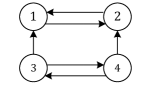
Figure 2: Network Topology of the multi-agent systems.

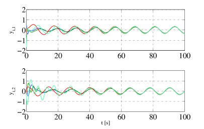
Figure 3: The synchronization of two output components $y_{i,1}$ and $y_{i,2}$

6 Conclusion

In the first part of the paper, we have identified a class of MIMO systems for which the $\gamma$-stabilization problem can be solved. In particular, we have proposed a static state feedback controller for the system in the normal form and a dynamic output feedback controller for a class of systems with a particular structure that arises from the robust output synchronization problem of MASs. In the second part of the paper, we have proposed a modified internal model design such that the robust output synchronization problem can be converted into perturbed consensus and perturbed regulation problems. The latter can be further converted to the $\gamma$-stabilization problem which can be solved by the dynamic output feedback controller developed in the first part. Overall, the robust output synchronization problem is solved by a distributed output feedback/communication controller integrating the techniques of reference model, internal model and $\gamma$-stabilization.

7 Appendix

Proof of Lemma 3.1: First, we note that $(\Phi_{0},\Gamma_{0})$ is controllable and $\Gamma_{0}\neq 0$ ($r_{0}>0$) by Assumption 3.1. We will prove the lemma using mathematical induction. Suppose, for $j\geq 0$, $(\Phi_{k},\Gamma_{k})$ is controllable and $\Gamma_{k}\neq 0$ (i.e., $r_{k}>0$) for $k=0,\cdots,j$. If $\Gamma_{j}$ has a full row rank, the lemma is true. Otherwise, the algorithm gives a valid pair of $(\Phi_{j+1},\Gamma_{j+1})$. Next, we aim to show that $(\Phi_{j+1},\Gamma_{j+1})$ is controllable and $\Gamma_{j+1}\neq 0$ (i.e., $r_{j+1}>0$).

Denote

$$Q(\lambda)=\left[\begin{array}[]{cc}\lambda I-\Phi_{j}&\Gamma_{j}\end{array}\right].$$

By PBH test, the fact that $(\Phi_{j},\Gamma_{j})$ is controllable implies that

$$\mbox{rank}(Q(\lambda))=n-\Sigma_{k=0}^{j-1}r_{k},\;\forall\lambda\in\mathbb{C}.$$

Let

$$\bar{Q}(\lambda)=U_{j+1}^{\mbox{\tiny{T}}}Q(\lambda)\left[\begin{array}[]{cc}U_{j+1}&\\ &H_{j+1}\end{array}\right].$$

One has $\mbox{rank}(\bar{Q}(\lambda))=\mbox{rank}(Q(\lambda))$ as $U_{j+1}$ and $H_{j+1}$ are unitary matrices. Direct calculation shows that

$$\bar{Q}(\lambda)=\left[\begin{array}[]{cccc}\lambda I-\tilde{U}_{j+1}^{\mbox{\tiny{T}}}\Phi_{j}\tilde{U}_{j+1}&-\tilde{U}_{j+1}^{\mbox{\tiny{T}}}\Phi_{j}\bar{U}_{j+1}&\Sigma_{j}&0\\ -\bar{U}_{j+1}^{\mbox{\tiny{T}}}\Phi_{j}\tilde{U}_{j+1}&\lambda I-\bar{U}_{j+1}^{\mbox{\tiny{T}}}\Phi_{j}\bar{U}_{j+1}&0&0\end{array}\right]$$

$$=\left[\begin{array}[]{cccc}\lambda I-\tilde{U}_{j+1}^{\mbox{\tiny{T}}}\Phi_{j}\tilde{U}_{j+1}&-\tilde{U}_{j+1}^{\mbox{\tiny{T}}}\Phi_{j}\bar{U}_{j+1}&\Sigma_{j}&0\\ -\Gamma_{j+1}&\lambda I-\Phi_{j+1}&0&0\end{array}\right].$$

Since $\Sigma_{j}$ has a full rank, i.e., $\mbox{rank}(\Sigma_{j})=r_{j}$, one has

$$\mbox{rank}\left(\left[\begin{array}[]{cc}\lambda I-\Phi_{j+1}&\Gamma_{j+1}\end{array}\right]\right)=\mbox{rank}(\bar{Q}(\lambda))-r_{j}=n-\Sigma_{k=0}^{j}r_{k},\;\forall\lambda\in\mathbb{C}.$$ (71)

Applying PBH test again shows that $(\Phi_{j+1},\Gamma_{j+1})$ is controllable and $\Gamma_{j+1}\neq 0$ (i.e., $r_{j+1}>0$).

From mathematical induction, for all $j\geq 0$, the pair $(\Phi_{j},\Gamma_{j})$ is well defined by the algorithm and controllable, until there is a finite number $l$ such that $\Gamma_{l}$ has a full row rank. Such a finite number $l$ always exists because the square matrix $\Phi_{j}$ of the dimension $n-\Sigma_{k=0}^{j-1}r_{k}$ with $r_{k}>0$ cannot be well defined for an arbitrarily large $j$.  

Proof of Lemma 3.2: Let

$$\bar{C}_{0}=C,\;\bar{C}_{j}=\bar{C}_{j-1}\bar{U}_{j},\;C_{j}=\bar{C}_{j-1}\tilde{U}_{j},\;j=1,\cdots,l.$$

Next, we will use mathematical induction to prove, for $j=1,\cdots,l$,

$${\rm Claim-}j:\;\;\left\{\begin{split}&\bar{C}_{k}\Phi_{k}^{j-1-k}\Gamma_{k}=0,\;k=0,\cdots,j-1\\ &C_{j}=0\end{split}\right..$$ (72)

For $j=1$, one has

$$CB=C\Gamma_{0}=C\tilde{U}_{1}\left[\begin{array}[]{cc}\Sigma_{0}&0\end{array}\right]H_{1}^{\mbox{\tiny{T}}}=0$$

by (12) and Assumption 3.2. Since both $\Sigma_{0}$ and $H_{1}$ are nonsingular, the above equations imply $C_{1}=C\tilde{U}_{1}=0$. Thus, Claim-$1$ is proved.

For $1\leq j\leq l-1$, we assume Claims-($1,\cdots,j$) hold and will prove Claim-$(j+1)$. Claims-($1,\cdots,j$) mean that

$$\left\{\begin{split}&\bar{C}_{k}\Phi_{k}^{s-1-k}\Gamma_{k}=0,\;k=0,\cdots,s-1\\ &C_{s}=0\end{split}\right.,\;\;s=1,\cdots,j.$$

that, with re-organization, implies

$$\left\{\begin{split}&\bar{C}_{k}\Phi_{k}^{s-1}\Gamma_{k}=0,\;s=1,\cdots,j-k\\ &C_{k}=0,\;\end{split}\right.,\;\;1\leq k\leq j.$$ (74)

With (74) in hand, we can prove the following implication

$$\bar{C}_{k-1}\Phi_{k-1}^{j-(k-1)}\Gamma_{k-1}=0\;\Longrightarrow\;\bar{C}_{k}\Phi_{k}^{j-k}\Gamma_{k}=0,\;1\leq k\leq j.$$ (75)

To prove (75), we denote

$$\Delta=\left[\begin{array}[]{c}\begin{array}[]{c}\tilde{U}_{k}^{\mbox{\tiny{T}}}\\ \bar{U}_{k}^{\mbox{\tiny{T}}}\end{array}\end{array}\right]\Phi_{k-1}\left[\begin{array}[]{cc}\tilde{U}_{k}&\bar{U}_{k}\end{array}\right]=\left[\begin{array}[]{cc}*&*\\ \Gamma_{k}&\Phi_{k}\end{array}\right].$$ (76)

Note that

$$\bar{C}_{k-1}\Phi_{k-1}^{j-(k-1)}\Gamma_{k-1} = \bar{C}_{k-1}\left[\begin{array}[]{cc}\tilde{U}_{k}&\bar{U}_{k}\end{array}\right]\Delta^{j-(k-1)}\left[\begin{array}[]{c}\begin{array}[]{c}\tilde{U}_{k}^{\mbox{\tiny{T}}}\\ \bar{U}_{k}^{\mbox{\tiny{T}}}\end{array}\end{array}\right]\left[\begin{array}[]{cc}\tilde{U}_{k}&\bar{U}_{k}\end{array}\right]\left[\begin{array}[]{cc}\Sigma_{k-1}&0\\ 0&0\end{array}\right]H_{k}^{\mbox{\tiny{T}}}$$

$$= \left[\begin{array}[]{cc}0&\bar{C}_{k}\end{array}\right]\Delta^{j-(k-1)}\left[\begin{array}[]{cc}\Sigma_{k-1}&0\\ 0&0\end{array}\right]H_{k}^{\mbox{\tiny{T}}}$$

where $C_{k}=\bar{C}_{k-1}\tilde{U}_{k}=0$ is used. Substituting (76) to the above equation and using the first equation of (74) lead to

$$\bar{C}_{k-1}\Phi_{k-1}^{j-(k-1)}\Gamma_{k-1}=\bar{C}_{k}\Phi_{k}^{j-k}\Gamma_{k}\left[\begin{array}[]{cc}\Sigma_{k-1}&0\end{array}\right]H_{k}^{\mbox{\tiny{T}}}=0.$$

So, one has $\bar{C}_{k}\Phi_{k}^{j-k}\Gamma_{k}=0$ as both $\Sigma_{k-1}$ and $H_{k}$ are nonsingular. The proof of (75) is thus complete.

By recursively using (75), Assumption 3.2, i.e., $CA^{j}B=\bar{C}_{0}\Phi_{0}^{j}\Gamma_{0}=0$ implies $\bar{C}_{1}\Phi_{1}^{j-1}\Gamma_{1}=0$, $\bar{C}_{2}\Phi_{2}^{j-2}\Gamma_{2}=0$, until $\bar{C}_{j}\Phi_{j}^{0}\Gamma_{j}=0$. In summary, $\bar{C}_{k}\Phi_{k}^{j-k}\Gamma_{k}=0,\;k=0,\cdots,j$.

Next, we note from (12) that

$$\bar{C}_{j}\Gamma_{j} = \bar{C}_{j}\left[\begin{array}[]{cc}\tilde{U}_{j+1}&\bar{U}_{j+1}\end{array}\right]\left[\begin{array}[]{cc}\Sigma_{j}&0\\ 0&0\end{array}\right]H_{j+1}^{\mbox{\tiny{T}}}$$

$$= C_{j+1}\left[\begin{array}[]{cc}\Sigma_{j}&0\end{array}\right]H_{j+1}^{\mbox{\tiny{T}}}=0$$

which implies $C_{j+1}=0$ as both $\Sigma_{j}$ and $H_{j+1}$ are nonsingular. From above, we have proved Claim-$(j+1)$.

For $j=2,\cdots,l+1$, one has $CT_{j}^{\mbox{\tiny{T}}}=C_{l-j+2}=0$ by Claim-$(l-j+2)$. Then

$$y=Cx=CT^{\mbox{\tiny{T}}}\zeta=CT_{1}^{\mbox{\tiny{T}}}\zeta_{1}+\sum_{j=2}^{l+1}CT_{j}^{\mbox{\tiny{T}}}\zeta_{j}=CT_{1}^{\mbox{\tiny{T}}}\zeta_{1}.$$

The proof is thus completed.

References

• [1] E.D. Sontag and Y. Wang. On characterizations of the input-to-state stability property. Systems & Control Letters, 24(5):351–359, 1995.
• [2] E.D. Sontag and Y. Wang. Notions of input to output stability. Systems & Control Letters, 38(4):235–248, 1999.
• [3] E.D. Sontag. Input to state stability: Basic concepts and results. In Nonlinear and optimal control theory, pages 163–220. Springer, 2008.
• [4] J.C. Doyle, K. Glover, P.P. Khargonekar, and B.A. Francis. State-space solutions to standard h/sub 2/and h/sub infinity/control problems. IEEE Transactions on Automatic control, 34(8):831–847, 1989.
• [5] A. Isidori and A. Astolfi. Disturbance attenuation and $H_{\infty}$-control via measurement feedback in nonlinear systems. IEEE Transactions on Automatic Control, 37(9):1283–1293, 1992.
• [6] A. Isidori and W. Kang. $H_{\infty}$ control via measurement feedback for general nonlinear systems. IEEE Transactions on Automatic Control, 40(3):466–472, 1995.
• [7] A. Van der Schaft. $L_{2}$-gain analysis of nonlinear systems and nonlinear state-feedback $H_{\infty}$ control. IEEE Transactions on Automatic Control, 37(6):770–784, 1992.
• [8] J. Ball, J. Helton, and W. Walker. $H_{\infty}$ control for nonlinear systems with output feedback. IEEE Transactions on Automatic Control, 38(4):546–559, 1993.
• [9] L. Zhu and Z. Chen. Robust input-to-output stabilization of nonlinear systems with a specified gain. Automatica, 84:199–204, 2017.
• [10] H.G. Tanner and D.K. Christodoulakis. Decentralized cooperative control of heterogeneous vehicle groups. Robotics and Autonomous Systems, 55(11):811 – 823, 2007.
• [11] A.E. Bergen and D.J. Hill. A structure preserving model for power system stability analysis. IEEE Transactions on Power Apparatus and Systems, (1):25–35, 1981.
• [12] P. Wieland, R. Sepulchre, and F. Allgøwer. An internal model principle is necessary and sufficient for linear output synchronization. Automatica, 47(5):1068 – 1074, 2011.
• [13] Y. Su and J. Huang. Cooperative output regulation with application to multi-agent consensus under switching network. IEEE Transactions on Systems, Man, and Cybernetics, Part B (Cybernetics), 42(3):864–875, 2012.
• [14] A. Isidori, L. Marconi, and G. Casadei. Robust output synchronization of a network of heterogeneous nonlinear agents via nonlinear regulation theory. IEEE Transactions on Automatic Control, 59(10):2680–2691, 2014.
• [15] L. Zhu, Z. Chen, and R. Middleton. Robust asymptotic model matching and its application to output synchronization of heterogeneous multi-agent systems. Systems & Control Letters, 94:37 – 45, 2016.
• [16] L. Zhu, Z. Chen, and R. H. Middleton. A general framework for robust output synchronization of heterogeneous nonlinear networked systems. IEEE Transactions on Automatic Control, 61(8):2092–2107, 2016.
• [17] Z. Chen. Pattern synchronization of nonlinear heterogeneous multiagent networks with jointly connected topologies. IEEE Transactions on Control of Network Systems, 1(4):349–359, 2014.
• [18] H. Kim, H. Shim, and J.H. Seo. Output consensus of heterogeneous uncertain linear multi-agent systems. IEEE Transactions on Automatic Control, 56(1):200–206, 2011.
• [19] A. Isidori. Nonlinear control systems. Springer Science & Business Media, 2013.
• [20] H.K. Khalil. Nonlinear systems, III. Prentice Hall, 2002.
• [21] Z. Chen and J. Huang. Stabilization and regulation of nonlinear systems. Springer, 2015.
• [22] Jie Huang. Nonlinear output regulation: theory and applications, volume 8. SIAM, 2004.
• [23] J.H. Seo, h. Shim, and J. Back. Consensus of high-order linear systems using dynamic output feedback compensator: low gain approach. Automatica, 45(11):2659–2664, 2009.