Event-triggered controllers based on the supremum norm of sampling-induced error

Abstract

The paper proposes a novel event-triggered control scheme for nonlinear systems. Specifically, the closed-loop system is associated with a pair of auxiliary input and output. The auxiliary output is defined as the derivative of the continuous-time input function, while the auxiliary input is defined as the input disturbance caused by the sampling or equivalently the integral of the auxiliary output over the sampling period. As a result, it forms a cyclic mapping from the input to the output via the system dynamics and back from the output to the input via the integral. The event-triggered law is constructed to make the mapping contractive such that the stabilization is achieved and an easy-to-check Zeno-free condition is provided. Within this framework, we develop a theorem for the event-triggered control of interconnected nonlinear systems which is employed to solve the event-triggered control for lower-triangular systems with dynamic uncertainties.

, , ,

1 Introduction

The majority of modern control systems reside in microprocessors and need more efficient implementation in order to reduce computation cost, save communication bandwidth and decrease energy consumption. Sampled-data control has been developed to fulfill these tasks where the execution of a digital controller is scheduled among sampling instances periodically or aperiodically. As a type of aperiodic sampling, event-triggered control suggests scheduling based on the state and/or sampling error of the plant and may achieve more efficient sampling pattern than periodic sampling. Event-triggered control has been developed for stabilization and tracking of individual systems, e.g., [30, 24, 29, 23] and cooperative control of networked systems, e.g., [14, 27, 10].

The two-step digital emulation is a common technique for analysis and design of sampled-data control systems especially for nonlinear systems. For periodic sampled-data control, it is an efficient tool to explicitly compute estimates of the maximum allowable sampling period (MASP) that guarantees asymptotic stability of sampled-data systems, e.g., [17, 26]. Emulation is also commonly adopted for the design of event-triggered laws where the continuous-time controller has been first proposed to make sure that the closed-loop system has the input-to-state stability (ISS) property, e.g., [3, 12, 23, 25, 22, 29], with the sampling error as the external input. The ISS condition was exploited in a max-form, e.g. [23] or in an ISS-Lyapunov form, e.g. [3, 22, 25, 29] for the closed-loop system with an emulated controller and the small gain conditions were proposed to ensure the stability of the event-triggered system. In [20], the event-triggered technique in [29] was interpreted as a stabilization problem of interconnected hybrid systems for which each subsystem admits an ISS-Lyapunov function and a hybrid small gain condition was proposed. As an other variant of small gain theorem, the cyclic small gain theorem has been proved effective for event-triggered control of large-scale systems [12, 22, 23]. Despite these progresses, design of event-triggered controllers that exclude Zeno behavior for complex nonlinear systems, such as interconnected systems where only states of some subsystems are available for the feedback, still remains a challenging problem.

The contribution of this paper is three-fold. First, a novel event-triggered control design method is proposed to achieve stabilization of individual and interconnected nonlinear systems. Specifically, the auxiliary output is defined as the derivative of the continuous-time feedback input function, and the auxiliary input is defined as the feedback input error caused by the sampling or equivalently the integral of the auxiliary output over the sampling period. Consequently, a closed-loop mapping is formed from the input to the output via the system dynamics and back from the output to the input via the integral function. The event-triggered law is constructed to make the mapping contractive, which is analogue to a small gain condition. The proposed method guarantees that the sampling interval approaches a constant as the system is stabilized. A similar approach was taken in [18], where the state and actuation sampling errors were utilized to construct the event-triggered law, while only the actuation sampling error is used in this paper. In [13, 2, 1, 26, 7], the periodic and event-triggered sampling relies on the calculation of MASP $T$ and requires the existence of a particular Lyapunov-like function on the hybrid systems.

Second, the event-triggered design method is used for the stabilization of interconnected nonlinear systems where only partial states are available for the feedback. In [22, 23], an auxiliary dynamic system was proposed to estimate the decay rate of immeasurable states as well as measurable states and used as the dynamic threshold for the event-triggered law. The new formulation in this paper allows to take the impact of the dynamic uncertainties explicitly into the event-triggered controller design and the proposed controller is static and are easier to design and implement in practice.

Third, we solve event-triggered control for lower-triangular nonlinear systems of relative degree greater than one using the proposed design method. The dynamic uncertainties are not directly manipulated by the controller and their states are not available for the feedback. The research [22] dealt with a simpler case where the dynamic uncertainties only appear at first relative degree level. In order to handle the higher relative degree, a new recursive recipe (backstepping technique) is designed to construct the event-triggered law.

Notation. Denote $\mathbb{R}^{n}$ the real coordinate space of $n$ dimensions. Denote $\mathbb{N}$ the set of non-negative integers, i.e., $\mathbb{N}=\{0,1,2,\cdots\}$. Denote $\mathbb{N}^{+}$ the set of positive integers and $\mathbb{R}^{+}$ the set of positive real numbers. Let $\|x_{[t_{1},t_{2}]}\|:=\sup_{t\in[t_{1},t_{2}]}\|x(t)\|$ for a given signal $x:\mathbb{R}\to\mathbb{R}^{n},n\in\mathbb{N}^{+}$. The symbol $\mbox{col}(z,x)=[z^{\mbox{\tiny{T}}},x^{\mbox{\tiny{T}}}]^{\mbox{\tiny{T}}}$ denotes the stacked vector by the vectors $z$ and $x$.

2 Main results

2.1 Event-Triggered Control Method

Consider a nonlinear system

$$\dot{x}(t)=f(x(t),u(t)),\;y(t)=h(x(t)),$$ (1)

where $x\in\mathbb{R}^{n}$ is the state, $y\in\mathbb{R}^{q}$ the output and $u\in\mathbb{R}^{m}$ the input. The continuous function $f:\mathbb{R}^{n}\times\mathbb{R}^{m}\to\mathbb{R}^{n}$ satisfies $f(0,0)=0$ such that $x=0$ is the equilibrium point of the system (1) when $u=0$. The function $h$ is continuously differentiable. Suppose stabilization of the equilibrium point can be fulfilled by the continuous-time state feedback controller

$$u(t)=g(y(t)),$$ (2)

with $g$ continuously differentiable where it is a continuous-time state feedback controller if $y(t)=x(t)$ or otherwise a continuous-time output feedback controller. In this paper, we will study the event-triggered version of (2) as follows

$$u(t)=g(y(t_{k})),\;t\in[t_{k},t_{k+1}),\;k\in\mathbb{N}$$ (3)

where $\{t_{k}\}_{k\in\mathbb{N}}$ is a sequence of sampling time instances and triggered by the condition

$$t_{k+1}=\inf_{t>t_{k}}\{\Xi(t_{k},y(t_{k}),y(t))>0\},\;k\in\mathbb{N}$$ (4)

with function $\Xi(t_{k},y(t_{k}),y(t))$ to be designed. The formulated event-triggered control system structure is illustrated in Fig. 1. The objective of event-triggered control is to design the triggering law (4) such that the closed-loop system composed of (1) and (3) achieves

1. Stabilization: the system is globally asymptotically stable at the origin.

2. Zeno-free Behavior: the infinitely fast sampling is avoided, i.e., $\inf_{k\in\mathbb{N}}\{t_{k+1}-t_{k}\}>0$ for any initial conditions.

The closed-loop system composed of (1) and (3) can be written as follows

$$\dot{x}(t)=f(x(t),g(y(t))-r(t)),$$ (5)

with the auxiliary input $r(t)$ and output $\xi(t)$ defined as follows

$$r(t)=\int_{t_{k}}^{t}\xi(s)ds,\;t\in[t_{k},t_{k+1}),\;\xi(t)=\frac{dg(y(t))}{dt}.$$ (6)

Different from most event-triggered control designs, the continuous-time feedback controller $g(y(t))$ in (2) is assumed to ensure that the closed-loop system has the following ISS and IOS conditions. Since $\xi$ relies on the actuation sampling error $r$ by its definition in (6), the IOS property characterizes the upper bound of $\|\xi(t)\|$ as a function of $\|r_{[t_{0},t]}\|$.

Assumption 2.1.

The closed-loop system (5) with $r$ as the piecewise continuous bounded external input and $\xi$ as the output has following input-to-state stability (ISS) and input-to-output stability (IOS) properties

$$\|x(t)\| \leq\max\{\tilde{\beta}(\|x(t_{0})\|,t-t_{0}),\tilde{\gamma}(\|r_{[t_{0},t]}\|)\},$$ (7)

$$\|\xi(t)\| \leq\max\{\beta(\|x(t_{0})\|,t-t_{0}),\gamma(\|r_{[t_{0},t]}\|)\},$$ (8)

for $t>t_{0}$ where $\beta,\tilde{\beta}\in\mathcal{KL}$ and $\gamma,\tilde{\gamma}\in\mathcal{K}_{\infty}$.

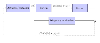
Figure 1: The formulated event-triggered control system structure.

Then, a new event-triggered control scheme is proposed as follows.

Theorem 2.1.

Consider the system (1) with the controller (3). Suppose the closed-loop system satisfies Assumption 2.1 and the gain function $\gamma$ satisfies

$$\lim_{s\rightarrow 0^{+}}\frac{\gamma(s)}{s}<\infty.$$ (9)

Let $\epsilon>1$ and $\bar{\gamma}$ be a $\mathcal{K}_{\infty}$ function satisfying

$$\bar{\gamma}(s)\geq\epsilon\gamma(s),\;\forall s>0\;\mbox{and}\;\lim_{s\rightarrow 0^{+}}\frac{\bar{\gamma}(s)}{s}=C_{s}$$ (10)

for some $C_{s}>0$. The objectives of the event-triggered control are achieved if the event-triggered law (4) is

$$t_{k+1}=\inf_{t>t_{k}}\{(t-t_{k})\bar{\gamma}(\|r_{[t_{k},t]}\|)>\|r_{[t_{k},t]}\|\},\;k\in\mathbb{N}$$ (11)

and Zeno-free behavior is achieved.

Proof: The closed-loop system (5) and (6) can be regarded as the interconnection of the $x$-subsystem and the $r$-subsystem noting that $p=x$ or $p=y$. The proof will be divided into four steps.

(1) Boundedness. We start with proving that $\|\xi(t)\|\leq R,\;\forall t\geq t_{0}$ for any given initial condition $x(t_{0})$ where $R:=\beta(\|x(t_{0})\|,0).$ If this is not true, there exists a finite time $T>0$ such that $\|\xi(T)\|>R$ and $\|\xi(t)\|\leq\bar{R}:=R+\Delta R,\forall t_{0}\leq t\leq T$ for a sufficiently small $\Delta R$. It will lead to the contradiction. Denote $\mathbb{S}_{T}:=\{k|k\in\mathbb{N}\mbox{ and }t_{0}\leq t_{k}\leq T$} the set of sampling steps within $[t_{0},T]$. Due to $C_{s}=\lim_{s\rightarrow 0^{+}}\bar{\gamma}(s)/s$, for a given $\delta$, there exists an $\epsilon$ such that $0<s<\epsilon\implies\left|\bar{\gamma}(s)/s-C_{s}\right|<\delta.$ Since $\xi(t)\leq\bar{R},\forall t\in[t_{0},T]$, one has $\|r_{[t_{k},t]}\|<\epsilon$ for any $t<t_{k}+\epsilon/\bar{R}$ due to the definition of $r(t)$ in (6). As a result, for $t<t_{k}+\epsilon/\bar{R}$, one has

$$\|r_{[t_{k},t]}\|<\epsilon\implies\left|\frac{\bar{\gamma}(\|r_{[t_{k},t]}\|)}{\|r_{[t_{k},t]}\|}-C_{s}\right|<\delta.$$

Consequently, the inequality leads to $\mu\bar{\gamma}(\|r_{[t_{k},t]}\|)<\|r_{[t_{k},t]}\|,\;\forall t<\epsilon/\bar{R}+t_{k}$ where $\mu=1/(C_{s}+\delta)$. Due to the event-triggered law (11), $t_{k+1}-t_{k}\geq\min\{1/(C_{s}+\delta),\epsilon/\bar{R}\}>0$. So, there exist finite sampling steps within the time duration $[t_{0},T]$. Due to $r(t)=\int_{t_{k}}^{t}\xi(s)ds,\;t\in[t_{k},t_{k+1}),$

$$\|r_{[t_{k},t]}\|\leq(t-t_{k})\|\xi_{[t_{k},t]}\|,\;\forall t\in[t_{k},t_{k+1})$$ (12)

Using inequality (12) and (8) leads to

$$\|\xi_{[t_{0},T]}\| \leq\max\{R,\bar{\gamma}(\|r_{[t_{0},t_{1}]}\|),\bar{\gamma}(\|r_{[t_{1},t_{2}]}\|),\cdots,\bar{\gamma}(\|r_{[t_{i},T]}\|)\}$$

$$\leq\max\{R,\frac{1}{t_{1}-t_{0}}\|r_{[t_{0},t_{1}]}\|,\frac{1}{t_{2}-t_{1}}\|r_{[t_{1},t_{2}]}\|,\cdots,$$

$$\quad\frac{1}{T-t_{i}}\|r_{[t_{i},T]}\|\}\leq R$$

which leads to a contradiction against $\xi(T)>R$. So, $\xi(t)$ is bounded, i.e., $\|\xi_{[t_{0},\infty)}\|\leq R$. It follows from (12) and (11) that

$$\bar{\gamma}(\|r_{[t_{k},t]}\|)\leq\|\xi_{[t_{k},t]}\|,\forall t\in[t_{k},t_{k+1}).$$ (13)

Thus, $r(t)$ and hence $x(t)$ are bounded for $t>t_{0}$ due to (7), i.e.,

$$\|x_{[t_{0},\infty)}\| \leq\max\{\tilde{\beta}(\|x(t_{0})\|,0),\tilde{\gamma}(\bar{\gamma}^{-1}(\beta(\|x(t_{0})\|,0)))\}$$

$$\|r_{[t_{0},\infty)}\| \leq\bar{\gamma}^{-1}(\beta(\|x(t_{0})\|,0))$$ (14)

(2) Zeno-free behavior. The avoidance of Zeno behavior follows from the proof of $\inf_{k\in\mathbb{N}}\{t_{k+1}-t_{k}\}>0,\forall k\in\mathbb{S}_{T}$ in the first step. We only need to replace the argument that $\xi(t)\leq R$ is bounded for $t\in[t_{0},T]$ with that $\xi(t)\leq R$ for $t>t_{0}$ and the set $\mathbb{S}_{T}$ with $\mathbb{N}$. And it also shows Zeno-free behavior can be achieved globally.

(3) Stability. The equilibrium point $x=0$ of the closed-loop system is stable, that is, for any $\delta>0$, there exists an $\epsilon$ such that if $\|x(t_{0})\|\leq\epsilon$ implies $\|x_{[t_{0},\infty)}\|\leq\delta$. From (14), it suffices to choose $\epsilon$ such that $\max\{\tilde{\beta}(\epsilon,0),\tilde{\gamma}(\bar{\gamma}^{-1}(\beta(\epsilon,0)))\}\leq\delta$ which is feasible.

(4) Convergence. The final step is to show that the state $x(t)$ approaches zero asymptotically $\lim_{t\rightarrow\infty}x(t)=0.$ Due to (10), one has

$$\inf_{s\in(0,r_{\infty})}\frac{\bar{\gamma}(s)}{s}\geq 1/T_{\max}$$ (15)

for some constant $T_{\max}<\infty$, which implies that $T_{\max}\bar{\gamma}(\|r_{[t_{k},t_{k}+T_{\max}]}\|)\geq\|r_{[t_{k},t+T_{\max}]}\|$ and thus

$$t_{k+1}-t_{k}\leq T_{\max},\;\forall t\in\mathbb{N},$$ (16)

i.e., $T_{\max}$ is the upper bound of the sampling interval. Consider the system behaviors of $\xi$ among interval $[t^{*}/2,t^{*}]$ for any $t^{*}>8T_{\max}$. First, inequality (8) with $t_{0}=t^{*}/4$ implies the signal $\|\xi_{[t^{*}/2,t^{*}]}\|$ satisfies

$$\|\xi_{[t^{*}/2,t^{*}]}\|\leq\max\{\beta(\|x(\frac{t^{*}}{4})\|,\frac{t^{*}}{4}),\gamma(\|r_{[t^{*}/4,t^{*}]}\|)\}.$$ (17)

Note that there exists integers $i,j$ such that $t^{*}/4\in[t_{i},t_{i+1}]$ where $t_{i}\geq t^{*}/8$, and $t^{*}\in[t_{j},t_{j+1}]$. Then, it follows from (17) and (10) that

$$\|\xi_{[t^{*}/2,t^{*}]}\|\leq\max\{\beta(\|x(\frac{t^{*}}{4})\|,\frac{t^{*}}{4}),1/\epsilon\bar{\gamma}(\|r_{[t_{i},t^{*}]}\|)\}$$

$$\leq\max\{\beta(\|x_{\infty}\|,\frac{t^{*}}{4}),1/\epsilon\|\xi_{[t^{*}/8,t^{*}/2]}\|\},$$ (18)

where the second inequality uses (11), the third one uses (12) and the last one uses $\|x_{[t_{0},\infty)}\|\leq x_{\infty}$. Denote $\zeta(t^{*})=\|\xi_{[t^{*}/2,t^{*}]}\|$, (18) can be rewritten as

$$\zeta(t^{*})\leq\max\{\beta(\|x_{\infty}\|,\frac{t^{*}}{4}),\frac{1}{\epsilon}\zeta(\frac{t^{*}}{2}),\frac{1}{\epsilon}\zeta(\frac{t^{*}}{4})\},$$ (19)

for all $t^{*}\geq 8T_{\max}.$ Next, we will show that $\lim_{t^{*}\rightarrow\infty}\zeta(t^{*})=0$. Otherwise, there exists a positive $\delta$ such that, for any $T$, there exists $t^{\ast}>T$ such that $\zeta(t^{*})>\delta$. Pick a positive integer $N$ satisfying

$$\delta\epsilon{}^{N}>R$$ (20)

and a $T$ such that $T/4^{N}>T_{\max},\;\beta(\|x_{\infty}\|,T/4^{N})<\delta.$ So, there exists $t^{*}>T$ such that $\zeta(t^{*})>\delta$. As a result,

$$\zeta(t^{*})>\delta>\beta(\|x_{\infty}\|,\frac{T}{4^{N}})>\beta(\|\Lambda_{\infty}\|,\frac{t^{*}}{4})$$

which together with (19) implies $\zeta(t^{*})\leq 1/\epsilon\zeta(\frac{t^{*}}{a_{1}}),\;\forall t^{*}\geq T$ where $a_{1}=2$ or $a_{1}=4$. By repeating this manipulation $N$ times, one has $\delta<\zeta(t^{*})\leq\left(\frac{1}{\epsilon}\right)^{N}\zeta(\frac{t^{*}}{a_{1}\cdots a_{N}}),\;\forall t^{*}\geq T.$ As a result, (20) further leads to $R<\delta\epsilon{}^{N}\leq\zeta(\frac{t^{*}}{a_{1}\cdots a_{N}}),$ which is a contradiction against $\xi(t)\leq R,\;\forall t\geq t_{0}$ proved in the second step. Consequently, the fact that $\lim_{t\rightarrow\infty}\zeta(t)=0$ holds which in turn implies $\lim_{t\rightarrow\infty}\xi(t)=0$, $\lim_{t\rightarrow\infty}r(t)=0$, and hence $\lim_{t\rightarrow\infty}x(t)=0$. Therefore, the system is asymptotically stable. Thus, Objective 1) and 2) of the event-triggered control are achieved globally (as the initial condition goes to infinity).  

Remark 2.1.

We can always select a function $\bar{\gamma}(s)$ that satisfies the condition (10) in Theorem (2.1). For instance, $\bar{\gamma}(s)=\epsilon_{1}\gamma(s)+\epsilon_{2}s$ for $\epsilon_{1}>1$ and $\epsilon_{2}>0$.

Remark 2.2.

The first step of the proof shows that the positive lower bound of the sampling interval depends on the initial conditions. In particular, it decreases when the norm of the system initial condition increases.

Remark 2.3.

The event-triggered law (11) leads to $\frac{\bar{\gamma}(\|r_{[t_{k},t]}\|)}{\|r_{[t_{k},t]}\|}\leq\frac{1}{(t-t_{k})},\forall t\in[t_{k},t_{k+1}).$ Note that the left hand side of the inequality is a nonlinear functional of the error $r$ and the right hand side is a time-varying threshold. It is similar to the event-triggered generated by a time-varying threshold in literature [15, 28].

Remark 2.4.

Let us consider the event-triggered control law (11) when the system is subject to the external disturbance $w(t)$,

$$\dot{x}(t)=f(x(t),u(t),w(t)),\;y(t)=h(x(t),w(t))$$ (21)

Suppose the system with $r$ in (6) as input and $\xi$ in (6) as the output has ISS and IOS properties, similar to Assumption 2.1,

$$\|x(t)\| \leq\max\{\tilde{\beta}(\|x(t_{0})\|,t-t_{0}),\tilde{\gamma}(\|r_{[t_{0},t]}\|),\tilde{\gamma}_{x}(\|w_{[t_{0},t]}\|)\}$$

$$\|\xi(t)\| \leq\max\{\beta(\|x(t_{0})\|,t-t_{0}),\gamma(\|r_{[t_{0},t]}\|),\gamma_{\xi}(\|w_{[t_{0},t]}\|)\},$$

for all $t>t_{0}$ where $\beta,\tilde{\beta}\in\mathcal{KL}$ and $\gamma,\tilde{\gamma},\tilde{\gamma}_{x},\gamma_{\xi}\in\mathcal{K}_{\infty}$. The event-triggered control law can achieve the following property of the closed-loop system viewing from the external disturbance $w$ to the state $x$, i.e.,

$$\|x(t)\|\leq\max\{\bar{\beta}(\|x(t_{0})\|,t-t_{0}),\tilde{\gamma}_{w}(\|w_{[t_{0},t]}\|)\},\;\forall t>t_{0}$$

for some functions $\bar{\beta}\in\mathcal{KL}$ and $\tilde{\gamma}_{w}\in\mathcal{K}_{\infty}$. The proof is similar to that in Theorem 2.1. The boundedness of system trajectories follows from the first part of the proof of Theorem 2.1. Zeno-free behavior relies on the existence of the limit $\lim_{s\rightarrow 0^{+}}\bar{\gamma}(s)/s$ and is not affected by the external disturbance. The proof of the property is similar to the proof of Theorem 3.2 in [8].

The following proposition shows that the sampling interval converges to a constant and the event-triggered control tends to be periodic sampling control as $t\rightarrow\infty$.

Proposition 2.1.

Consider the event-triggered law (11) in Theorem 2.1. Suppose $\mu:=\lim_{s\rightarrow 0^{+}}\bar{\gamma}(s)/s>0$ and $T=1/\mu$. Then, $\lim_{k\rightarrow\infty}t_{k+1}-t_{k}=T$ for all initial conditions.

Proof: The idea of this proof is to show that $\lim_{k\rightarrow\infty}t_{k+1}-t_{k}=T$ as $r(t)$ approaches zero when $t$ goes to infinity. Note that it suffices to prove for any $\delta^{*}$ there exists a $k^{*}$ such that $|t_{k+1}-t_{k}-T|<\delta^{*}$, $\forall k\geq k^{*}$. Without loss of generality, we only consider the case of $\delta^{*}<T$. Due to $\lim_{s\rightarrow 0^{+}}\bar{\gamma}(s)/s=1/T$, for any $\delta>0$, there exists an $\epsilon$ such that

$$\|r_{[t_{k},t]}\|<\epsilon\implies\left|\frac{\bar{\gamma}(\|r_{[t_{k},t]}\|)}{\|r_{[t_{k},t]}\|}-1/T\right|<\delta.$$ (22)

Due to $\lim_{t\rightarrow\infty}r(t)=0$ by Theorem 2.1, for any $\delta_{1}>0$, there exists $t(\delta_{1})$ such that $t>t(\delta_{1})\implies\|r(t)\|<\delta_{1}$. In what follows, we consider the behavior of $r(t)$ for $t>t(\delta_{1})$. Let

$$0<\delta<\min\{\frac{\delta^{*}}{T^{2}+T\delta^{*}},\frac{\delta^{*}}{T^{2}-T\delta^{*}}\}.$$ (23)

We choose $\delta_{1}\leq\epsilon$ such that $\|r(t)\|<\epsilon$ is satisfied for $t>t(\delta_{1})$ and $k^{*}$ such that $t(k^{*})>t(\delta_{1})$. Consequently, (22) implies $T/(1+T\delta)\gamma(\|r_{[t_{k},t]}\|)<\|r_{[t_{k},t]}\|$ and $T/(1-T\delta)\gamma(\|r_{[t_{k},t]}\|)>\|r_{[t_{k},t]}\|,\;\forall k\geq k^{*},$ which, together with the event-triggered law (11), shows that $T/(1-T\delta)>t_{k+1}-t_{k}>T/(1+T\delta).$ By the selection of $\delta$ in (23), one has

$$\delta^{*}>\frac{T^{2}\delta}{1-T\delta}>t_{k+1}-t_{k}-T>-\frac{T^{2}\delta}{1+T\delta}>-\delta^{*},$$

which implies that $|t_{k+1}-t_{k}-T|<\delta^{*}$, $\forall k\geq k^{*}$. Thus, the proof is complete.  

Remark 2.5.

For a linear function $\gamma$ and thus $\bar{\gamma}$, the event-triggered law (11) directly leads to a periodic sampling scheme.

2.2 Interconnected Systems

In this section, we consider event-triggered control of a nonlinear interconnected system described as follows

$$\dot{z}(t) =q(z(t),x(t),u(t)),$$

$$\dot{x}(t) =f(z(t),x(t),u(t)),$$ (24)

where $z\in\mathbb{R}^{q}$ and $x\in\mathbb{R}^{n}$ are the states of the two subsystems, and $u\in\mathbb{R}^{m}$ is the input. The continuous functions $q:\mathbb{R}^{q}\times\mathbb{R}^{n}\times\mathbb{R}^{m}\to\mathbb{R}^{q}$ and $f:\mathbb{R}^{q}\times\mathbb{R}^{n}\times\mathbb{R}^{m}\to\mathbb{R}^{n}$ satisfy $q(0,0,0)=0$ and $f(0,0,0)=0$ such that $\mbox{col}(z,x)=0$ is the equilibrium point of the overall system with $u=0$. The state $z$ is assumed not available for the feedback. The aim is to construct an event-triggered controller (3) such that the system is globally asymptotically stable at $\mbox{col}(z,x)=0$ and Zeno-free behavior is achieved. This problem was solved in [22] using the cyclic small gain theorem. Here, we will adopt the new event-triggered control scheme proposed in Section 2.1 to solve the problem and explicitly characterize how the $z$-dynamics affect the event-triggered control law.

The closed-loop system composed of (24) and (3) can be written as follows

$$\dot{z}(t) =q(z(t),x(t),g(x(t))-r(t)),$$

$$\dot{x}(t) =f(z(t),x(t),g(x(t))-r(t)),$$ (25)

with the auxiliary input $r(t)$ and output $\xi(t)$ defined as follows

$$r(t)=\int_{t_{k}}^{t}\xi(s)ds,\;t\in[t_{k},t_{k+1}),\;\xi(t)=\frac{dg(x(t))}{dt}.$$ (26)

The following ISS and bounded state and input to bounded output (BSIBO) conditions are assumed for the closed-loop system (25). The assumptions could be matched through proper controller design in some real applications, for example, the specific design approach is discussed in Section 3 for lower-triangular systems.

Assumption 2.2.

The closed-loop system (25) with $r$ as the piecewise continuous bounded external input and $\xi$ as the output has following ISS properties.

• The $z$-dynamics and $x$-dynamics are ISS, i.e.,

  $$\|z(t)\|\leq \max\{\beta_{z}(\|z(t_{0})\|,t-t_{0}),\gamma_{z}^{x}(\|x_{[t_{0},t]}\|),$$

  $$\gamma_{z}^{r}(\|r_{[t_{0},t]}\|)\},\;\forall t>t_{0}$$ (27)

  $$\|x(t)\|\leq \max\{\beta_{x}(\|x(t_{0})\|,t-t_{0}),\gamma_{x}^{z}(\|z_{[t_{0},t]}\|),$$

  $$\gamma_{x}^{r}(\|r_{[t_{0},t]}\|)\},\;\forall t>t_{0}$$ (28)

  for some functions $\beta_{x},\beta_{z}\in\mathcal{KL}$ and $\gamma_{z}^{x},\gamma_{z}^{r},\gamma_{x}^{z},\gamma_{x}^{r}\in\mathcal{K}_{\infty}$.

• It is BSIBO viewing $z$ and $x$ as states, $r$ as the input and $\xi$ as the output, i.e.,

  $$\|\xi(t)\|\leq \max\{\gamma_{\xi}^{z}(\|z_{[t_{0},t]}\|),\gamma_{\xi}^{x}(\|x_{[t_{0},t]}\|),\gamma_{\xi}^{r}(\|r_{[t_{0},t]}\|)\},$$

  $$\qquad\qquad\qquad\qquad\qquad\qquad\forall t>t_{0}$$ (29)

  for some functions $\gamma_{\xi}^{z},\gamma_{\xi}^{x},\gamma_{\xi}^{r}\in\mathcal{K}_{\infty}$.

A useful lemma is presented as follows.

Lemma 2.1.

([31]) Consider the system (25) with $\Lambda=[z^{\mbox{\tiny{T}}},x^{\mbox{\tiny{T}}}]^{\mbox{\tiny{T}}}$. Suppose $r(t)$ is the piecewise continuous bounded input. If (27) and (27) hold and the small gain condition $\gamma_{z}^{x}\circ\gamma_{x}^{z}(s)<s,\;\forall s>0$ is satisfied, the system (25) is ISS in the sense of

$$\|z(t)\| \leq\max\{\bar{\beta}_{z}(\|\Lambda(t_{0})\|,t-t_{0}),\bar{\gamma}_{z}^{r}(\|r_{[t_{0},t]}\|)\},$$ (30)

$$\|x(t)\| \leq\max\{\bar{\beta}_{x}(\|\Lambda(t_{0})\|,t-t_{0}),\bar{\gamma}_{x}^{r}(\|r_{[t_{0},t]}\|)\},$$ (31)

for all $t\geq t_{0}$ where $\bar{\beta}_{\zeta},\bar{\beta}_{\chi}\in\mathcal{KL}$ and class $\mathcal{K}_{\infty}$ functions $\bar{\gamma}_{z}^{r}=\max\{\gamma_{z}^{r},\gamma_{z}^{x}\circ\gamma_{x}^{r}\},\;\bar{\gamma}_{x}^{r}=\max\{\gamma_{x}^{r},\gamma_{x}^{z}\circ\gamma_{z}^{r}\}.$

Remark 2.6.

As in [22], we deliberately consider the ISS property for the $z$ and $x$-dynamics separately rather than consider that for $\Lambda=[z^{\mbox{\tiny{T}}},x^{\mbox{\tiny{T}}}]^{\mbox{\tiny{T}}}$ as a whole. On one hand, it facilitates examination of $z$ and $x$-dynamics’ individual effect on the event-triggered control design. On the other hand, under the small gain condition $\gamma_{z}^{x}\circ\gamma_{x}^{z}(s)<s,\;\forall s>0$, we can derive the ISS property for the $\Lambda$-dynamics

$$\|\Lambda(t)\|\leq\max\{\beta_{\Lambda}(\|\Lambda(t_{0})\|,t-t_{0}),\gamma_{\Lambda}(\|r_{[t_{0},t]}\|)\},$$ (32)

for all $t\geq t_{0}$ where $\beta_{\Lambda}\in\mathcal{KL}$ and $\gamma_{\Lambda}:=2\max\{\bar{\gamma}_{z}^{r},\bar{\gamma}_{x}^{r}\}\\ \in\mathcal{K}_{\infty}$. By Lemma 2.1, we can use the ISS properties (30) and (31) with less conservative gain functions $\bar{\gamma}_{z}^{r}$ and $\bar{\gamma}_{x}^{r}$ instead of (32) with $\gamma_{\Lambda}$ to design the event-triggered law. As will be explained in Remark 2.8, it may lead to a better sampling pattern.

Theorem 2.2.

Consider the system (24) with the controller (3). Suppose Assumption 2.2 is satisfied with the small gain condition $\gamma_{z}^{x}\circ\gamma_{x}^{z}(s)<s,\forall s>0.$ Let $\gamma:=\max\{\gamma_{\xi}^{z}\circ\bar{\gamma}_{z}^{r},\gamma_{\xi}^{x}\circ\bar{\gamma}_{x}^{r},\gamma_{\xi}^{r}\}$ where $\bar{\gamma}_{x}^{r}$ and $\bar{\gamma}_{z}^{r}$ are given in Lemma 2.1. Suppose $\gamma$ satisfies

$$\lim_{s\rightarrow 0^{+}}\frac{\gamma(s)}{s}<\infty.$$ (33)

Let $\epsilon>1$ and $\bar{\gamma}$ be a $\mathcal{K}_{\infty}$ function satisfying

$$\bar{\gamma}(s)\geq\epsilon\gamma(s),\;\forall s>0\;\mbox{and}\;\lim_{s\rightarrow 0^{+}}\frac{\bar{\gamma}(s)}{s}>0.$$ (34)

The objectives of the event-triggered control are achieved if the event-triggered law (4) is

$$t_{k+1}=\inf_{t>t_{k}}\{(t-t_{k})\bar{\gamma}(\|r_{[t_{k},t]}\|)>\|r_{[t_{k},t]}\|\},\;k\in\mathbb{N}$$ (35)

where $r$ is define in (26).

Proof: By Lemma 2.1, one has (30) and (31). Following the similar argument in Theorem 2.1, we can prove signals $x(t)$, $z(t)$, $r(t)$ and $\xi(t)$ of the closed-loop system (25) are bounded. Since all signals are bounded, we can substitute (30) and (31) into (29) and obtain

$$\|\xi(t)\|\leq\max\{\beta(\|\Lambda(t_{0})\|,t-t_{0}),\gamma(\|r_{[t_{0},t]}\|)\}$$ (36)

for all $t\geq t_{0}$, where $\beta\in\mathcal{KL}$. Note that (30), (31) and (36) are similar to conditions of Theorem 2.1. The rest of the proof directly follows that of Theorem 2.1.  

Remark 2.7.

Let us consider two special cases: (1) $x$ and $u$ do not appear in the $z$-dynamics, i.e., $\dot{z}(t)=q(z(t)),\;\dot{x}(t)=f(x(t),z(t),u(t))$ ($\gamma_{z}^{x}=\gamma_{z}^{r}=0$); (2) $u$ does not appear in the $z$-dynamics but $x$ does, and $z$ does not appear in $x$-dynamics, i.e, $\dot{z}(t)=q(z(t),x(t)),\;\dot{x}(t)=f(x(t),u(t))$ ($\gamma_{z}^{r}=\gamma_{x}^{z}=\gamma_{\xi}^{z}=0$). It follows from Theorem 2.2 that $\bar{\gamma}(s)$ in (34) should be

$$\bar{\gamma}(s)\geq\epsilon\gamma(s):=\epsilon\max\{\gamma_{\xi}^{x}\circ\gamma_{x}^{r}(s),\gamma_{\xi}^{r}(s)\}.$$

As opposed to the method in [22], we explicitly show that the variation of $z$-dynamics does not affect Zeno-free behavior for both aforementioned cases. Specifically, in both cases, it is not necessary to re-design the event-triggered law (35) when the $z$-dynamics vary.

Remark 2.8.

For a function $\gamma$, it is observed from (35) that less conservative selection of $\bar{\gamma}(s)$ may increase the sampling interval $t_{k+1}-t_{k}$, which could lead to a desirable sampling pattern that less number of control executions are taken within a given period. If the ISS property (32) is used to derive an event-triggered law rather than (30) and (31), we can derive the following inequality similar to (36),

$$\|\xi(t)\|\leq\max\{\beta(\|\Lambda(t_{0})\|,t-t_{0}),\tilde{\gamma}(\|r_{[t_{0},t]}\|)\},$$ (37)

for $t\geq t_{0}$ with $\tilde{\gamma}:=\max\{\gamma_{\xi}\circ\gamma_{\Lambda},\gamma_{\xi}^{r}\}$ where $\gamma_{\xi}=\max\{\gamma_{\xi}^{x},\gamma_{\xi}^{z}\}$ and $\gamma_{\Lambda}:=2\max\{\bar{\gamma}_{z}^{r},\bar{\gamma}_{x}^{r}\}$. It follows from the proof of Theorem 2.2 that $\bar{\gamma}(s)$ should be

$$\bar{\gamma}(s)\geq\epsilon\tilde{\gamma}(s).$$ (38)

The fact $\tilde{\gamma}(s)>\gamma(s)$ makes the choice of $\bar{\gamma}(s)$ more conservative.

3 Lower-Triangular Systems

3.1 Problem Formulation

In this section, we consider the event-triggered control for a class of lower-triangular systems

$$\dot{z}_{j}(t) =q_{j}(\vec{z}_{j}(t),\vec{x}_{j}(t),w),$$

$$\dot{x}_{j}(t) =f_{j}(\vec{z}_{j}(t),\vec{x}_{j}(t),w)+b_{j}x_{j+1},\;j=1,\cdots,\ell$$ (39)

where $\vec{z}_{j}:=\mbox{col}(z_{1},\cdots,z_{j})$ and $\vec{x}_{j}:=\mbox{col}(x_{1},\cdots,x_{j})$ are the states, $u:=x_{\ell+1}$ is the control input, $b_{j}$’s are constants and $\ell$ is the relative degree. Note that $z_{j}\in\mathbb{R}^{n_{j}}$ and $x_{j}\in\mathbb{R}$. $w\in\mathbb{W}$ represents system uncertainties (such as unknown parameters) in a known compact set $\mathbb{W}$, while $\vec{z}_{j}$-dynamics are called dynamic uncertainties where the function $q_{j}$’s are not precisely known and $\vec{z}_{j}$ is not available for feedback. Note that $w$ can be time-varying. The functions $q_{j}$ and $f_{j}$ are assumed to be sufficiently smooth and satisfy $q_{j}(0,0,w)=0$ and $f_{j}(0,0,w)=0$. The continuous-time stabilization of such system has been solved using the Lyapunov function method [11] and the small gain theorem [16] based on backstepping technique. In the spirit of backstepping, we introduce the coordinate transformation

$$\bar{x}_{1} =x_{1}$$

$$\bar{x}_{j} =x_{j}-\vartheta_{j-1}(\bar{x}_{j-1}),\;j=2,\cdots,\ell+1$$ (40)

where the functions $\vartheta_{1},\cdots,\vartheta_{\ell}$ satisfying $\vartheta_{i}(0)=0$ are virtual controllers to be designed at each recursive step. Under the coordinate (40), the system (39) becomes

$$\dot{z}_{j}(t) =\bar{q}_{j}(\vec{z}_{j}(t),\vec{\bar{x}}_{j}(t),w)$$

$$\dot{\bar{x}}_{j}(t) =\bar{f}_{j}(\vec{z}_{j}(t),\vec{\bar{x}}_{j}(t),w)+\vartheta_{j}(\bar{x}_{j}(t))+\bar{x}_{j+1}(t),$$

$$\quad\quad\quad\quad j=1,\cdots,\ell$$ (41)

where $\vec{\bar{x}}_{j}:=\mbox{col}(\bar{x}_{1},\cdots,\bar{x}_{j})$, $\bar{q}_{j}(\vec{z}_{j},\vec{\bar{x}}_{j},w)$ and $\bar{f}_{j}(\vec{z}_{j},\vec{\bar{x}}_{j},w)$ are sufficiently smooth functions satisfying $\bar{q}_{j}(0,0,w)=0$ and $\bar{f}_{j}(0,0,w)=0$. For continuous-time stabilization, the controller is of the form $u=x_{\ell+1}=\vartheta_{\ell}(\bar{x}_{\ell})$ by setting $\bar{x}_{\ell+1}=0$. For event-triggered control, we adopt the method developed in Section 2 and propose the controller as follows

$$u(t)=\vartheta_{\ell}(\bar{x}_{\ell}(t_{k}))\mbox{ or }u(t)=\vartheta_{\ell}(\bar{x}_{\ell}(t))-\bar{x}_{\ell+1}(t)$$ (42)

where $\bar{x}_{\ell+1}(t)$ is the sampling error defined as

$$\bar{x}_{\ell+1}(t)=\int_{t_{k}}^{t}\xi(s)ds,\;t\in[t_{k},t_{k+1}),\;\xi(t)=\frac{d\vartheta_{\ell}(\bar{x}_{\ell}(t))}{dt}.$$ (43)

with the triggering law to be designed as

$$t_{k+1}=\inf_{t>t_{k}}\{\Xi(t_{k},\vec{\bar{x}}_{\ell}(t_{k}),\vec{\bar{x}}_{\ell}(t))>0\},\;k\in\mathbb{N}.$$ (44)

The backstepping controller design (40) is a classic continuous-time stabilization technique for lower-triangular nonlinear systems. For event-triggered control, the continuous-time controller $u(t)=\vartheta_{\ell}(\bar{x}_{\ell}(t))$ needs to be designed such that the closed-loop system has an ISS gain from state sampling error $e(t):=\vec{x}_{\ell}(t)-\vec{x}_{\ell}(t_{k})$ to states $\vec{x}_{\ell}$ and $\vec{z}_{\ell}$ for existing event-triggered control design or from actuation error $\bar{x}_{\ell+1}(t)$ to states for the controller in this paper. We will design a new recursive recipe to separate the ISS properties of $\vec{\bar{x}}_{\ell}$ and $\vec{z}_{\ell}$ for the closed-loop system (41) and employ Theorem 2.2 to design the event-triggered law (44). The traditional treatment in the literature mixes $\vec{z}_{j}$ and $\vec{\bar{x}}_{j}$-dynamics and derives the ISS property for $\|\mbox{col}(\vec{z}_{j}(t),\vec{\bar{x}}_{j}(t))\|$ as a whole at each recursive step. In the spirit of the design method in Section 2.2, we separately consider the $\vec{z}_{j}$ and $\vec{\bar{x}}_{j}$-dynamics at each step to derive the following ISS properties. In particular, we aim to design the continuous-time controllers $\vartheta_{1},\cdots,\vartheta_{\ell}$ such that the following statement holds for $j=1,\cdots,\ell$.

Statement $j$: The $(\vec{z}_{j},\vec{\bar{x}}_{j})$-dynamics of (41) are ISS in the sense of

$$\|\vec{z}_{j}(t)\| \leq\max\{\bar{\beta}_{Z_{j}}(\|\mbox{col}(\vec{z}_{j}(t_{0}),\vec{\bar{x}}_{j}(t_{0}))\|,t-t_{o}),$$

$$\quad\bar{\gamma}_{Z_{j}}^{x_{j+1}}(\|\bar{x}_{j+1}\|)\},$$

$$\|\vec{\bar{x}}_{j}(t)\| \leq\max\{\bar{\beta}_{X_{j}}(\|\mbox{col}(\vec{z}_{j}(t_{0}),\vec{\bar{x}}_{j}(t_{0}))\|,t-t_{o}),$$

$$\quad\bar{\gamma}_{X_{j}}^{x_{j+1}}(\|\bar{x}_{j+1}\|)\},\;\forall t\geq t_{0}$$ (45)

for some functions $\bar{\beta}_{Z_{j}},\bar{\beta}_{X_{j}}\in\mathcal{KL}$ and $\bar{\gamma}_{Z_{j}}^{x_{j+1}},\bar{\gamma}_{X_{j}}^{x_{j+1}}\in\mathcal{K}_{\infty}$ to be calculated. Furthermore, the gain functions satisfy

$$\bar{\gamma}_{X_{j}}^{x_{j+1}}(s)<s\;\mbox{ and }\lim_{s\rightarrow 0^{+}}\frac{\bar{\gamma}_{Z_{j}}^{x_{j+1}}(s)}{s}<\infty,\;\forall s>0.$$ (46)

3.2 Recursive Controller Design

We will propose the event-triggered controller under a standard assumption.

Assumption 3.1.

The $z_{j}$-subsystem for $j=1,\cdots,\ell$ in (39) is ISS for all $w\in\mathbb{W}$ viewing $z_{j}$ as state, $\vec{z}_{j-1}$ and $\vec{x}_{j}$ as inputs with the ISS functions $\gamma_{z_{j}}^{z},\gamma_{z_{j}}^{x}\in\mathcal{K}_{\infty}$ satisfying $\lim_{s\rightarrow 0^{+}}\gamma_{z_{j}}^{z}(s)/s<\infty$ and $\lim_{s\rightarrow 0^{+}}\gamma_{z_{j}}^{x}(s)/s<\infty$, respectively.

Remark 3.1.

Under Assumption 3.1, the $z_{j}$-subsystem in (41) is ISS viewing $z_{j}$ as state and $\mbox{col}(\vec{z}_{j-1},\vec{\bar{x}}_{j})$ as input, in particular,

$$\|z_{j}(t)\|\leq \max\big{\{}\beta_{z_{j}}(|z_{j}(t_{0})|,t-t_{0}),\gamma_{z_{j}}^{z}(\|\vec{z}{}_{j-1[t_{0},t]}\|),$$

$$\quad\bar{\gamma}_{z_{j}}^{x}(\|\vec{\bar{x}}_{j[t_{0},t]}\|)\big{\}},\;\forall t>t_{0}$$ (47)

for some functions $\beta_{z_{j}}\in\mathcal{KL}$ and $\bar{\gamma}_{z_{j}}^{x}\in\mathcal{K}_{\infty}$ with $\lim_{s\rightarrow 0^{+}}\bar{\gamma}_{z_{j}}^{x}(s)/s<\infty.$

For $w\in\mathbb{W}$, direct calculation leads to

$$|\bar{f}_{1}(z_{1},\bar{x}_{1},w)|\leq\iota_{1}(|z_{1}|)|z_{1}|+m_{1}(\bar{x}_{1})|\bar{x}_{1}|,$$ (48)

and, for $j=2,\cdots,\ell$,

$$|\bar{f}_{j}(\vec{z}_{j},\vec{\bar{x}}_{j},w)|< \iota_{j}(\|\vec{z}_{j}\|)\|\vec{z}_{j}\|+\tilde{m}_{j}(\|\vec{\bar{x}}_{j-1}\|)\|\vec{\bar{x}}_{j-1}\|$$

$$+m_{j}(\bar{x}_{j})|\bar{x}_{j}|,$$ (49)

where we select non-negative sufficiently smooth functions $\iota_{j}$, $m_{j}$ and $\tilde{m}_{j}$. Denote

$$\bar{\iota}_{j}(s)=\frac{1}{4c_{j}}\iota_{j}^{2}(s)s^{2},\;j=1,\cdots,\ell$$

$$\bar{c}_{1}=c_{1},\;\bar{c}_{j}=2c_{j},\;\bar{m}_{j}(s)=\frac{1}{4c_{j}}\tilde{m}_{j}^{2}(s)s^{2},\;j=2,\cdots,\ell$$

for constants $c_{j}>0$. Define $\gamma_{Z_{j}}^{X_{j}}=2\max\{\bar{\gamma}_{z_{j}}^{x},\bar{\gamma}_{Z_{j-1}}^{x_{j}},\gamma_{z_{j}}^{z}\circ\bar{\gamma}_{Z_{j-1}}^{x_{j}}\},\;j=2,\cdots,\ell.$ The continuous-time stabilization controller is designed as follows

$$\vartheta_{j}(\bar{x}_{j})=-(\bar{c}_{j}+\frac{1}{4}b_{j}^{2}+m_{j}(\bar{x}_{j})+\psi_{j}(|\bar{x}_{j}|))\bar{x}_{j}/b_{j},\;j=1,\cdots,\ell$$ (50)

where we select some sufficiently smooth and even functions $\psi_{j}(s)$ satisfying the following conditions

$$\psi_{1}(s)>k_{1}\max\{\bar{\iota}_{1}\circ\gamma_{z_{1}}^{x}(s)/s^{2},1\}$$

$$\psi_{j}(s)>k_{j}\max\{\bar{m}_{j}(s)/s^{2},\bar{\iota}_{j}\circ\gamma_{Z_{j}}^{X_{j}}(2s)/s^{2},2\}$$ (51)

for $k_{1}>2$ and $k_{j}>3,\;j=2,\cdots,\ell$.

Lemma 3.1.

Consider the closed-loop system composed of (39) and (42) with any piecewise bounded external input $\bar{x}_{j+1}$. Let $\vartheta_{j}(\bar{x}_{j})$, for $j=1,\cdots,\ell$, be given in (50). Then, Statement $j$ holds for $j=1,\cdots,\ell$.

Proof: We will use mathematical induction to prove Statement $j$. For step $j=1$. Let $V_{1}(\bar{x}_{1})=\bar{x}_{1}^{2}/2$ be a Lyapunov function candidate for $\bar{x}_{1}$-subsystem. Then, one has

$$\dot{V}_{1}(\bar{x}_{1}) =\bar{x}_{1}[f_{1}(z_{1},\bar{x}_{1},w)+\bar{x}_{2}+\vartheta_{1}(\bar{x}_{1})]$$

$$\leq-\rho_{1}(|\bar{x}_{1}|)+\bar{\iota}_{1}(|z_{1}|)+\bar{x}_{2}^{2}$$

for a class $\mathcal{K}_{\infty}$ function $\rho_{1}(s)=\psi_{1}(s)s^{2}$ where we used (50) and (48). As a result, the $\bar{x}_{1}$-dynamics are ISS viewing $\bar{x}_{1}$ as state and $\mbox{col}(z_{1},\bar{x}_{2})$ as input, in particular,

$$|\bar{x}_{1}(t)|\leq \max\big{\{}\beta_{x_{1}}(|\bar{x}_{1}(t_{0})|,t-t_{0}),\gamma_{x_{1}}^{z}(\|z_{1}\|),$$

$$\gamma_{x_{1}}^{x_{2}}(\|\bar{x}_{2}\|)\big{\}},\forall t>t_{0}$$ (52)

where $\gamma_{x_{1}}^{z}=\rho_{1}^{-1}\circ(k_{1}\bar{\iota}_{1})$ and $\gamma_{x_{1}}^{x_{2}}(s)=\rho_{1}^{-1}(k_{1}s^{2})$. According to (47), we have

$$\|z_{1}(t)\|\leq\max\left\{\beta_{z_{1}}(\|z_{1}(t_{o})\|,t-t_{0}),\bar{\gamma}_{z_{1}}^{x}(\|\bar{x}_{1}\|)\right\},\forall t>t_{0}.$$ (53)

Choosing $\psi_{1}(s)$ in (51) leads to the small gain condition $\gamma_{x_{1}}^{z}\circ\gamma_{z_{1}}^{x}(s)=\rho_{1}^{-1}\circ(k_{1}\bar{\iota}_{1})\circ\bar{\gamma}_{z_{1}}^{x}(s)<s$ and $\gamma_{x_{1}}^{x_{2}}(s)=\rho_{1}^{-1}(k_{1}s^{2})<s.$ By Lemma 2.1, the $(z_{1},\bar{x}_{1})$-dynamics are ISS in the sense of (45) with $\bar{\gamma}_{X_{1}}^{x_{2}}=\gamma_{x_{1}}^{x_{2}},\;\bar{\gamma}_{Z_{1}}^{x_{2}}=\bar{\gamma}_{z_{1}}^{x}\circ\gamma_{x_{1}}^{x_{2}}.$ Due to $\lim_{s\rightarrow 0^{+}}\bar{\gamma}_{z_{1}}^{x}(s)/s<\infty,$ one can find the function $\rho_{1}\in\mathcal{K}$ and the function $\psi_{1}(s)$ satisfying (51). Also, one has $\lim_{s\rightarrow 0^{+}}\bar{\gamma}_{Z_{1}}^{x_{2}}(s)/s<\infty$, i.e., (46) is satisfied for $j=1$. Statement $j$ holds for $j=1$.

For step $j\geq 2$. It is noted that the $(\vec{z}_{j},\vec{\bar{x}}_{j})$-system is composed of the $(\vec{z}_{j-1},\vec{\bar{x}}_{j-1})$-subsystem, the $\bar{x}_{j}$-subsystem, and the $z_{j}$-subsystem. For the purpose of induction, suppose that $\vartheta_{j-1}(\bar{x}_{j-1})$ has been designed such that Statement $j-1$ holds. Then, we aim to design $\vartheta_{j}(\bar{x}_{j})$ in this step such that Statement $j$ also holds. Let $V_{j}=\bar{x}_{j}^{2}/2$ be a Lyapunov function candidate for $\bar{x}_{j}$-subsystem. Then, one has

$$\dot{V}_{j}(\bar{x}_{j})=\bar{x}_{j}[\bar{f}_{j}(\vec{z}_{j},\vec{\bar{x}}_{j},w)+\bar{x}_{j+1}+\nu_{j}(\bar{x}_{j})]$$

$$\leq-\rho_{j}(\bar{x}_{j})+\bar{\iota}_{j}(\|\vec{z}_{j}\|)+\bar{m}_{j}(\|\vec{\bar{x}}_{j-1}\|)+\bar{x}_{j+1}^{2}$$

for a class $\mathcal{K}_{\infty}$ function $\rho_{j}(s)=\psi_{j}(s)s^{2}$ where we used (50) and (49). As a result, the $\bar{x}_{j}$-dynamics are ISS viewing $\bar{x}_{j}$ as state and $\mbox{col}(\vec{z}_{j},\vec{\bar{x}}_{j-1},\bar{x}_{j+1})$ as input, in particular,

$$|\bar{x}_{j}(t)|\leq \max\big{\{}\beta_{x_{j}}(|x_{j}(t_{0})|,t-t_{0}),\gamma_{x_{j}}^{z}(\|\vec{z}_{j}\|),\gamma_{x_{j}}^{x}(\|\vec{\bar{x}}_{j-1}\|),$$

$$\gamma_{x_{j}}^{x_{j+1}}(|\bar{x}_{j+1}|)\big{\}},\;\forall t>t_{0}$$ (54)

where $\gamma_{x_{j}}^{z}=\rho_{j}^{-1}\circ(k_{j}\bar{\iota}_{j}),\;\gamma_{x_{j}}^{x}=\rho_{j}^{-1}\circ(k_{j}\bar{m}_{j}),\;\gamma_{x_{j}}^{x_{j+1}}(s)=\rho_{j}^{-1}(k_{j}s^{2}).$ According to (47), one has

$$\|z_{j}(t)\|\leq \max\big{\{}\bar{\beta}_{z_{j}}(|z_{j}(t_{0})|,t-t_{0}),\gamma_{z_{j}}^{z}(\|\vec{z}_{j-1}\|),\bar{\gamma}_{z_{j}}^{x}(\|\vec{\bar{x}}_{j}\|)\big{\}},$$

$$\qquad\qquad\qquad\qquad\qquad\qquad\forall t>t_{0}.$$ (55)

Consider class $\mathcal{K}$ functions $\bar{\gamma}_{Z_{j-1}}^{x_{j}}$, $\bar{\gamma}_{Z_{j-1}}^{\sigma}$, $\bar{\gamma}_{X_{j-1}}^{x_{j}}$, and $\bar{\gamma}_{X_{j-1}}^{\sigma}$ from Statement $j-1$. Choosing $\psi_{j}(s)$ in (51) leads to small gain condition $\gamma_{x_{j}}^{x}\circ\bar{\gamma}_{X_{j-1}}^{x_{j}}(s)=\rho_{j}^{-1}\circ(k_{j}\bar{m}_{j})\circ\bar{\gamma}_{X_{j-1}}^{x_{j}}(s)\leq\rho_{j}^{-1}\circ(k_{j}\bar{m}_{j})(s)<s$ by noting $\bar{\gamma}_{X_{j-1}}^{x_{j}}(s)<s$. Define

$$\gamma_{Z_{j}}^{X_{j}} =2\max\{\bar{\gamma}_{z_{j}}^{x},\bar{\gamma}_{Z_{j-1}}^{x_{j}},\gamma_{z_{j}}^{z}\circ\bar{\gamma}_{Z_{j-1}}^{x_{j}}\}$$

$$\gamma_{X_{j}}^{Z_{j}} =2\gamma_{x_{j}}^{z},\;\gamma_{X_{j}}^{x_{j+1}}=2\gamma_{x_{j}}^{x_{j+1}}.$$

Using (51), one has the other small gain condition

$$\gamma_{Z_{j}}^{X_{j}}\circ\gamma_{X_{j}}^{Z_{j}}(s)=\gamma_{Z_{j}}^{X_{j}}\circ(2\gamma_{x_{j}}^{z})(s)=\gamma_{Z_{j}}^{X_{j}}\circ(2\rho_{j}^{-1})\circ(k_{j}\bar{\iota}_{j})(s)<s$$

By Lemma 3.2 in [31], the $(\vec{z}_{j},\vec{\bar{x}}_{j})$-dynamics are ISS in the sense of (45), with

$$\bar{\gamma}_{Z_{j}}^{x_{j+1}}=\gamma_{Z_{j}}^{X_{j}}\circ\gamma_{X_{j}}^{x_{j+1}},\;\bar{\gamma}_{X_{j}}^{x_{j+1}}=\gamma_{X_{j}}^{x_{j+1}},$$

and $\bar{\gamma}_{X_{j}}^{x_{j+1}}(s)=2\rho_{j}^{-1}(k_{j}s^{2})<s$ due to (51). Due to $\lim_{s\rightarrow 0^{+}}\bar{\gamma}_{z_{j}}^{x}(s)/s<\infty,$ $\lim_{s\rightarrow 0^{+}}\bar{\gamma}_{Z_{j-1}}^{x_{j}}(s)/s<\infty,$ and $\lim_{s\rightarrow 0^{+}}\gamma_{z_{j}}^{z}(s)/s<\infty,$ one has $\lim_{s\rightarrow 0^{+}}\gamma_{Z_{j}}^{X_{j}}(s)/s<\infty.$ One can always find a function $\rho_{i}\in\mathcal{K}_{\infty}$ and a function $\psi_{j}(s)$ satisfying (51). Also, one can verify (46) for Statement $j$. The proof for Statement $j=2,\cdots,\ell$ is thus complete.  

3.3 Event-Triggered Control

Note that Statement $\ell$ implies that

$$\|\vec{z}_{\ell}(t)\|\leq \max\{\bar{\beta}_{Z_{\ell}}(\|\mbox{col}(\vec{z}_{\ell}(t_{0}),\vec{\bar{x}}_{\ell}(t_{0}))\|,t-t_{o}),$$

$$\bar{\gamma}_{Z_{\ell}}^{x_{\ell+1}}(\|\bar{x}_{\ell+1}\|)\},$$

$$\|\vec{\bar{x}}_{\ell}(t)\|\leq \max\{\bar{\beta}_{X_{\ell}}(\|\mbox{col}(\vec{z}_{\ell}(t_{0}),\vec{\bar{x}}_{\ell}(t_{0}))\|,t-t_{o}),$$

$$\bar{\gamma}_{X_{\ell}}^{x_{j+1}}(\|\bar{x}_{\ell+1}\|)\},\;\forall t\geq t_{0}.$$ (56)

Remark 3.2.

Note from (56) that $\bar{x}_{\ell+1}=\vartheta_{\ell}(\bar{x}_{\ell}(t))-\vartheta_{\ell}(\bar{x}_{\ell}(t_{k}))=\bar{\vartheta}_{\ell}(\vec{x}_{\ell}(t_{k})+e)-\bar{\vartheta}_{\ell}(\vec{x}_{\ell}(t_{k}))$ for some function $\bar{\vartheta}$ where $e(t):=\vec{x}_{\ell}(t)-\vec{x}_{\ell}(t_{k})$. Then, there exists a class $\mathcal{K}$ function $\tilde{\vartheta}$ such that $\bar{x}_{\ell+1}\leq\tilde{\vartheta}(\|q\|)$. Therefore, the recursive controller design presented in Section 3.2 can also render the closed-loop system have an ISS gain from state sampling error $e$ to $\vec{x}_{\ell}$ and $\vec{z}_{\ell}$. By separating ISS gains from $e$ to $\vec{x}_{\ell}$ and $\vec{z}_{\ell}$, it is possible to design the event-triggered controller that only utilized partial state $\vec{x}_{\ell}$, as was done in [22].

Therefore, the ISS property from the auxiliary input $\bar{x}_{\ell+1}$ to $\mbox{col}(\vec{z}_{\ell}(t),\vec{\bar{x}}_{\ell}(t))$ is achieved, which is similar to have the conditions (27) and (28) in Assumption 2.2 satisfied, by applying Lemma 2.1. We also need to verify (29) in order to use Theorem 2.2. For this purpose, let us examine the auxiliary output $\xi$ in (43). Note that

$$\xi(t)=\frac{d\vartheta_{\ell}(\bar{x}_{\ell})}{d\bar{x}_{\ell}}\dot{\bar{x}}_{\ell}=\alpha(\bar{x}_{\ell})[\bar{f}_{\ell}(\vec{z}_{\ell},\vec{\bar{x}}_{\ell},w)+\bar{x}_{\ell+1}+\vartheta_{\ell}(\bar{x}_{\ell})]$$

where $\alpha(\bar{x}_{\ell}):=\frac{d\vartheta_{\ell}(\bar{x}_{\ell})}{d\bar{x}_{\ell}}$. From $\vartheta_{\ell}(\bar{x}_{\ell})$ in (50), one has

$$\alpha(\bar{x}_{\ell})= -(\bar{c}_{\ell}+\frac{1}{4}b_{\ell}^{2}+m_{\ell}(\bar{x}_{\ell})+\psi_{\ell}(|\bar{x}_{\ell}|))/b_{\ell}$$

$$+\left(\frac{dm_{\ell}(\bar{x}_{\ell})}{d\bar{x}_{\ell}}+\frac{d\psi_{\ell}(|\bar{x}_{\ell}|)}{d\bar{x}_{\ell}}\right)\bar{x}_{\ell}/b_{\ell}=c+\kappa_{1}(\bar{x}_{\ell})$$

for some constant $c$ and sufficiently smooth function $\kappa_{1}$ satisfying $\kappa_{1}(0)=0$. Since $\bar{f}_{\ell}(\vec{z}_{\ell},\vec{\bar{x}}_{\ell},w)$ is sufficiently smooth, one has

$$|\bar{f}_{\ell}(\vec{z}_{\ell},\vec{\bar{x}}_{\ell},w)+\vartheta_{\ell}(\bar{x}_{\ell})+\bar{x}_{\ell+1}|<$$

$$\kappa_{2}(\|\vec{z}_{\ell}\|)\|\vec{z}_{\ell}\|+\kappa_{3}(\|\vec{\bar{x}}_{\ell}\|)\|\vec{\bar{x}}_{\ell}\|+|\bar{x}_{\ell+1}|$$ (57)

for some non-negative sufficiently smooth functions $\kappa_{2}$ and $\kappa_{3}$. As a result, there exist $\gamma_{\xi}^{z},\gamma_{\xi}^{x}\in\mathcal{K}_{\infty}$ satisfying $\lim_{s\rightarrow 0^{+}}\gamma_{\xi}^{z}(s)/s<\infty$ and $\lim_{s\rightarrow 0^{+}}\gamma_{\xi}^{x}(s)/s<\infty$ such that $\|\xi(t)\|\leq\max\{\gamma_{\xi}^{z}(\|\vec{z}_{\ell}\|),\gamma_{\xi}^{x}(\|\vec{\bar{x}}_{\ell}\|),\gamma_{\xi}^{r}(|\bar{x}_{\ell+1}|)\},$ where $\gamma_{\xi}^{r}(|\bar{x}_{\ell+1}|)=\alpha|\bar{x}_{\ell+1}|^{2}+\beta|\bar{x}_{\ell+1}|$ for some constants $\alpha,\beta>0$. It thus verifies (29). Finally, we can check that $\lim_{s\rightarrow 0^{+}}\gamma_{\xi}^{z}(s)/s<\infty$, $\lim_{s\rightarrow 0^{+}}\gamma_{\xi}^{x}(s)/s<\infty$, $\lim_{s\rightarrow 0^{+}}\bar{\gamma}_{Z_{j}}^{x_{j+1}}(s)/s<\infty$, $\lim_{s\rightarrow 0^{+}}\bar{\gamma}_{X_{j}}^{x_{j+1}}(s)/s<\infty$ and hence $\lim_{s\rightarrow 0^{+}}\gamma(s)/s<\infty.$

By Theorem 2.2, the conclusion on the event-triggered controller is drawn as follows.

Theorem 3.1.

Consider the closed-loop system composed of (39) and (42) where $\vartheta_{j}(\bar{x}_{j})$, for $j=1,\cdots,\ell$, is given in (50). Suppose the closed-loop system satisfies Assumption 3.1. Let $\epsilon>1$ and $\bar{\gamma}\in\mathcal{K}_{\infty}$ be

$$\bar{\gamma}(s)\geq\epsilon\gamma(s),\;\forall s>0\;$$ (58)

where $\gamma(s):=\max\{\gamma_{\xi}^{z}\circ\bar{\gamma}_{Z_{j}}^{x_{j+1}}(s),\gamma_{\xi}^{x}\circ\bar{\gamma}_{X_{j}}^{x_{j+1}}(s),\gamma_{\xi}^{r}(s)\}$ and $\bar{\gamma}_{Z_{j}}^{x_{j+1}},\bar{\gamma}_{X_{j}}^{x_{j+1}}$ are given in (45).The objectives of event-trigger control are achieved if the event-triggered law in (44) is

$$t_{k+1}=\inf_{t>t_{k}}\{(t-t_{k})\bar{\gamma}(\|r_{[t_{k},t]}\|)>\|r_{[t_{k},t]}\|\},\;k\in\mathbb{N}.$$ (59)

4 Numerical Simulation

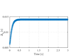
Figure 2: Triggering instants under the designed scheme for the system (60).

Consider the following lower-triangular system

$$\dot{z}_{1}(t) =-z_{1}^{3}(t)$$

$$\dot{x}_{1}(t) =w_{1}z_{1}(t)+x_{2}(t)$$

$$\dot{z}_{2}(t) =-z_{2}(t)+x_{1}(t)$$

$$\dot{x}_{2}(t) =-w_{2}x_{1}(t)x_{2}(t)+x_{1}(t)+3u$$ (60)

where $[z_{1},x_{1},z_{2},x_{2}]^{\mbox{\tiny{T}}}$ are states and $w_{1},w_{2}\in[0,1]$ are the parameter uncertainties. The $z_{1}$ and $z_{2}$-dynamics represent dynamic uncertainties. We will use Theorem 3.1 to design the event-triggered controller. Applying Lemma 3.1, the continuous-time stabilization controller is designed as $u=\vartheta_{2}(\bar{x}_{2})=-(0.3\bar{x}_{2}^{2}+5)\bar{x}_{2}$ where $\bar{x}_{2}=x_{2}+2.5x_{1}.$ Also, we obtain $\bar{\gamma}_{Z_{2}}^{x_{3}}=2s$, $\bar{\gamma}_{X_{2}}^{x_{3}}=s$. The bound of $\xi(t)$ can be calculated as follows

$$|\xi(t)|=\left|\frac{d\vartheta_{2}(\bar{x}_{2})}{d\bar{x}_{2}}\dot{\bar{x}}_{2}\right|\leq\max\{\gamma_{\xi}^{z}(\|\vec{z}_{2}\|),\gamma_{\xi}^{x}(\|\vec{\bar{x}}_{2}\|),\gamma_{\xi}^{r}(\|r\|)\}$$

with $\gamma_{\xi}^{z}(s)=2.5s^{2}+12.5s$, $\gamma_{\xi}^{x}(s)=0.27s^{5}+3.56s^{4}+15s^{3}+40s^{2}+70s$, and $\gamma_{\xi}^{r}(s)=s^{2}+5s$. The calculation shows that $\gamma(s)$ in (58) is $\gamma(s)=\gamma_{\xi}^{x}(s)$ and it satisfies $\lim_{s\rightarrow 0^{+}}\gamma(s)/s<\infty.$ Let $\bar{\gamma}(s)$ in (58) be $\bar{\gamma}(s)=1/0.99\gamma(s)$. Then, the event-triggered law (59) can achieve the stabilization without Zeno behavior. Figure 2 shows that the sampling interval $\Delta_{k}=t_{k+1}-t_{k}$ converges to $0.0141$s as $t\rightarrow\infty$, due to $\lim_{s\rightarrow 0^{+}}\bar{\gamma}(s)/s=70.7$ (by Proposition 2.1) and no Zeno behavior occurs. Figure 3 shows that the state asymptotically goes to zero. Note that $z_{1}$-dynamics do not converge to zero exponentially and the triggering law using exponentially converging threshold signals may lead to Zeno behavior (see Example 2 in [22]), while the proposed controller does not. Next, let us compare the proposed event-triggered law and periodic sampling with sampling interval being $0.0141$s when the initial condition is $[z_{1},x_{1},z_{2},x_{2}]^{\mbox{\tiny{T}}}=[-19.67,23.09,-24.77,13.755]^{\mbox{\tiny{T}}}$. The simulation in Figure 4 shows that the proposed event-triggered law can stabilize the system while the periodic sampling does not. This is consistent with result in [9] that the sampling interval required to stabilize the plant depends on initial condition.

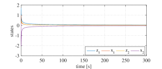
Figure 3: Simulation profiles of the event-triggered control for the system (60)

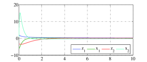
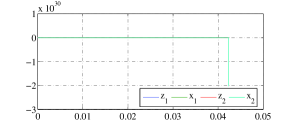
Figure 4: The simulation comparison in Section 4: proposed event-triggered law (upper) and periodic sampling with sampling interval being 0.0141 (lower) for initial condition $[z_{1},x_{1},z_{2},x_{2}]^{\mbox{\tiny{T}}}=[-19.67,23.09,-24.77,13.755]^{\mbox{\tiny{T}}}$.

5 Conclusion

In this paper, a novel event-triggered control scheme for nonlinear systems was proposed. Then, it was applied to develop a theorem for the event-triggered control of interconnected nonlinear systems. We also provided an easy-to-check Zeno-free condition and showed that the sampling interval converges to a constant as time approaches infinity. Then, we employed the theorem to solve the event-triggered control for lower-triangular systems with dynamic uncertainties. It remains an interesting future direction to consider the robustness of the proposed with respect to more imperfections, such as measurement noise in [6, 13, 5], state quantization in [21], modeling uncertainties in [19], time delays in [4], and so on.

References

- [1] M. Abdelrahim, R. Postoyan, J. Daafouz, and D. Nešić. Robust event-triggered output feedback controllers for nonlinear systems. Automatica, 75:96–108, 2017.
- [2] M. Abdelrahim, R. Postoyan, J. Daafouz, D. Nešić, and W. P. M. H. Heemels. Co-design of output feedback laws and event-triggering conditions for the L2 -stabilization of linear systems. Automatica, 87(87):337–344, 2018.
- [3] A. Anta and P. Tabuada. To sample or not to sample: Self-triggered control for nonlinear systems. IEEE Transactions on Automatic Control, 55(9):2030–2042, 2010.
- [4] D. P. Borgers, V. S. Dolk, and W. P. M. H. Heemels. Riccati-based design of event-triggered controllers for linear systems with delays. IEEE Transactions on Automatic Control, 63(1):174–188, 2018.
- [5] D. P. Borgers, R. Postoyan, A. Anta, P. Tabuada, D. Nešić, and W. P. M. H. Heemels. Periodic event-triggered control of nonlinear systems using overapproximation techniques. Automatica, 94(94):81–87, 2018.
- [6] F. D. Brunner, W. P. M. H. Heemels, and F. Allgöwer. Event-triggered and self-triggered control for linear systems based on reachable sets. Automatica, 101:15–26, 2019.
- [7] D. Carnevale, A. R. Teel, and D. Nesic. A lyapunov proof of an improved maximum allowable transfer interval for networked control systems. IEEE Transactions on Automatic Control, 52(5):892–897, 2007.
- [8] X. Chen and Z. Chen. Robust sampled-data output synchronization of nonlinear heterogeneous multi-agents. IEEE Transactions on Automatic Control, 62(3):1458–1464, 2016.
- [9] Z. Chen and H. Fujioka. Performance analysis of nonlinear sampled-data emulated controllers. IEEE Transactions on Automatic Control, 59(10):2778–2783, 2014.
- [10] Z. Chen, Q.-L. Han, Y. Yan, and Z.-G. Wu. How often should one update control and estimation: review of networked triggering techniques. Science China Information Sciences, 63:150201:1–18, 2020.
- [11] Z. Chen and J. Huang. Dissipativity, stabilization, and regulation of cascade-connected systems. IEEE Transactions on Automatic Control, 49(5):635–650, 2004.
- [12] C. De Persis, R. Sailer, and F. Wirth. On a small-gain approach to distributed event-triggered control. IFAC Proceedings Volumes, 44(1):2401–2406, 2011.
- [13] V. S. Dolk, D. P. Borgers, and W. P. M. H. Heemels. Output-based and decentralized dynamic event-triggered control with guaranteed - gain performance and zeno-freeness. IEEE Transactions on Automatic Control, 62(1):34–49, 2017.
- [14] Y. Fan, G. Feng, Y. Wang, and C. Song. Distributed event-triggered control of multi-agent systems with combinational measurements. Automatica, 49(2):671–675, 2013.
- [15] M. Guinaldo, D. V. Dimarogonas, K. H. Johansson, J. Sanchez, and S. Dormido. Distributed event-based control strategies for interconnected linear systems. IET Control Theory and Applications, 7(6):877–886, 2013.
- [16] Z. P. Jiang and I. M. Y. Mareels. A small-gain control method for nonlinear cascaded systems with dynamic uncertainties. IEEE Transactions on Automatic Control, 42(3):292–308, 1997.
- [17] I. Karafyllis and C. Kravaris. Global stability results for systems under sampled-data control. International Journal of Robust and Nonlinear Control, 19(10):1105–1128, 2009.
- [18] Z. Khan, G. D.and Chen and L. Zhu. A new approach for event-triggered stabilization and output regulation of nonlinear systems. IEEE Transactions on Automatic Control, 2019.
- [19] M. Kishida. Event-triggered control with self-triggered sampling for discrete-time uncertain systems. IEEE Transactions on Automatic Control, 64(3):1273–1279, 2019.
- [20] D. Liberzon, D. Nešić, and A. R. Teel. Lyapunov-based small-gain theorems for hybrid systems. IEEE Transactions on Automatic control, 59(6):1395–1410, 2014.
- [21] T. Liu and Z. Jiang. Event-triggered control of nonlinear systems with state quantization. IEEE Transactions on Automatic Control, 64(2):797–803, 2019.
- [22] T. Liu and Z. P. Jiang. Event-based control of nonlinear systems with partial state and output feedback. Automatica, 53:10–22, 2015.
- [23] T. Liu and Z. P. Jiang. A small-gain approach to robust event-triggered control of nonlinear systems. IEEE Transactions on Automatic Control, 60(8):2072–2085, 2015.
- [24] N. Marchand, S. Durand, and J. F. G. Castellanos. A general formula for event-based stabilization of nonlinear systems. IEEE Transactions on Automatic Control, 58(5):1332–1337, 2013.
- [25] M. Mazo, A. Anta, and P. Tabuada. An iss self-triggered implementation of linear controllers. Automatica, 46(8):1310–1314, 2010.
- [26] D. Nesic, A. R. Teel, and D. Carnevale. Explicit computation of the sampling period in emulation of controllers for nonlinear sampled-data systems. IEEE Transactions on Automatic Control, 54(3):619–624, 2009.
- [27] G. S. Seyboth, D. V. Dimarogonas, and K. H. Johansson. Event-based broadcasting for multi-agent average consensus. Automatica, 49(1):245–252, 2013.
- [28] G. S. Seyboth, D. V. Dimarogonas, and K. H. Johansson. Event-based broadcasting for multi-agent average consensus. Automatica, 49(1):245–252, 2013.
- [29] P. Tabuada. Event-triggered real-time scheduling of stabilizing control tasks. IEEE Transactions on Automatic Control, 52(9):1680–1685, 2007.
- [30] P. Tallapragada and N. Chopra. On event triggered tracking for nonlinear systems. IEEE Transactions on Automatic Control, 58(9):2343–2348, 2013.
- [31] L. Zhu and Z. Chen. Robust input-to-output stabilization of nonlinear systems with a specified gain. Automatica, 84:199 – 204, 2017.