Low-rank geometric mean metric learning

Abstract

We propose a low-rank approach to learning a Mahalanobis metric from data. Inspired by the recent geometric mean metric learning (GMML) algorithm, we propose a low-rank variant of the algorithm. This allows to jointly learn a low-dimensional subspace where the data reside and the Mahalanobis metric that appropriately fits the data. Our results show that we compete effectively with GMML at lower ranks.

1 Introduction

We propose a scalable solution for the Mahalanobis metric learning problem (Kulis, 2012). The Mahalanobis distance is defined as $d_{\mathbf{A}}(\mbox{\boldmath$x$},\mbox{\boldmath$x^{\prime}$})=(\mbox{\boldmath$x$}-\mbox{\boldmath$x^{\prime}$})^{\top}\mathbf{A}(\mbox{\boldmath$x$}-\mbox{\boldmath$x^{\prime}$})$, where $\mbox{\boldmath$x$},\mbox{\boldmath$x^{\prime}$}\in\mathbb{R}^{d}$ are input vectors and $\mathbf{A}$ is a $d\times d$ symmetric positive definite (SPD) matrix. The objective is to learn a suitable SPD matrix $\mathbf{A}$ from the given data. Since $\mathbf{A}$ is a $d\times d$ SPD matrix, most state-of-the-art metric learning algorithms scale poorly with the number of features $d$ (Harandi et al., 2017). To mitigate this, a pre-processing step of dimensionality reduction (e.g., by PCA) is generally applied before using popular algorithms like LMNN and ITML (Weinberger & Saul, 2009; Davis et al., 2007).

Recently, (Zadeh et al., 2016) proposed the geometric mean metric learning (GMML) formulation, which enjoys a closed-form solution. However, it requires matrix $\mathbf{A}$ to be positive definite, which makes it unscalable in a high dimensional setting. To alleviate this concern, we propose a low-rank decomposition of $\mathbf{A}$ in the GMML setting. Low-rank constraint also has a natural interpretation in the metric learning setting, since the group of similar points in the given dataset reside in a low-dimensional subspace. We jointly learn the low-dimensional subspace along with the metric. We show that the optimization is on the Grassmann manifold and propose a computationally efficient algorithm. On real-world datasets, we achieve competitive results comparable with the GMML algorithm, even though we work on a smaller dimensional space.

2 Problem formulation

We follow a weekly supervised approach in which we are provided two sets $\mathcal{S}$ and $\mathcal{D}$ containing pairs of input points belonging to same and different classes respectively. Taking inspiration from GMML, we formulate the objective function as:

$$\begin{array}[]{ll}\min\limits_{\mathbf{A}\succeq 0}&\operatorname{Tr}(\mathbf{AS})+\operatorname{Tr}(\mathbf{A^{\dagger}D})\\ {\rm subject\ to}&{\rm rank}(\mathbf{A})=r,\end{array}$$ (1)

where $\mathbf{S}:=\sum_{(\mbox{\boldmath$x$}_{i},\mbox{\boldmath$x$}_{j})\in\mathcal{S}}{(\mbox{\boldmath$x$}_{i}-\mbox{\boldmath$x$}_{j})(\mbox{\boldmath$x$}_{i}-\mbox{\boldmath$x$}_{j})^{\top}}$, $\mathbf{D}:=\sum_{(\mbox{\boldmath$x$}_{i},\mbox{\boldmath$x$}_{j})\in\mathcal{D}}{(\mbox{\boldmath$x$}_{i}-\mbox{\boldmath$x$}_{j})(\mbox{\boldmath$x$}_{i}-\mbox{\boldmath$x$}_{j})^{\top}}$, and $\mathbf{A^{\dagger}}$ is the pseudoinverse of $\mathbf{A}$.

Exploiting a particular fixed-rank factorization (Meyer et al., 2011), we factorize rank-$r$ matrix $\mathbf{A}$ as $\mathbf{A}=\mathbf{UBU}^{\top}$, where $\mathbf{U}$ is an orthonormal matrix of size $d\times r$ and $\mathbf{B}\succ 0$ is of size $r\times r$. Consequently, we rewrite (1) as:

$$\min\limits_{\mathbf{U}^{\top}\mathbf{U}=\mathbf{I}}\ \min\limits_{\mathbf{B}\succ 0}\quad\operatorname{Tr}(\mathbf{UBU^{\top}S})+\operatorname{Tr}(\mathbf{U}\mathbf{B}^{-1}\mathbf{U}^{\top}\mathbf{D}).$$ (2)

If we define $\mathbf{\widetilde{S}}=\mathbf{U^{\top}SU}$ and $\mathbf{\widetilde{D}}=\mathbf{U^{\top}DU}$, then the inner minimization problem with respect to $\mathbf{B}$ has a closed-form solution as the geometric mean of ${\mathbf{\widetilde{S}}}^{-1}$ and $\mathbf{\widetilde{D}}$ (Zadeh et al., 2016), i.e., $\mathbf{B}=\mathbf{\widetilde{S}}^{-1/2}(\mathbf{\widetilde{S}}^{1/2}\mathbf{\widetilde{D}}\mathbf{\widetilde{S}}^{1/2})^{1/2}\mathbf{\widetilde{S}}^{-1/2}$. Using this fact, the outer optimization problem is readily checked to be only on the column space of $\mathbf{U}$. To see this, consider the group action $\mathbf{U}\mapsto\mathbf{UO}$, where $\mathbf{O}$ is an $r$-by-$r$ orthogonal matrix. For all $\mathbf{O}$, this group action captures the column space of $\mathbf{U}$. The mapping $\mathbf{U}\mapsto\mathbf{UO}$ implies that $\mathbf{B}\mapsto\mathbf{O}^{\top}\mathbf{BO}$ and consequently, the objective function in (2) remains invariant to all $\mathbf{O}$.

The set of column spaces is the abstract Grassmann manifold ${\rm Grass}(r,d)$, which is defined as the set of $r$-dimensional subspaces in $\mathbb{R}^{d}$. We represent the abstract column space of $\mathbf{U}$ as $\mathcal{U}$. Equivalently, (2) is formulated as:

$$\begin{array}[]{lll}\min\limits_{\mathcal{U}\in{\rm Grass}(r,d)}&f(\mathcal{U}),\end{array}$$ (3)

where $f(\mathcal{U}):=\min\limits_{\mathbf{B}\succ 0}\operatorname{Tr}(\mathbf{UBU^{\top}S})+\operatorname{Tr}(\mathbf{U}\mathbf{B}^{-1}\mathbf{U}^{\top}\mathbf{D})$. Optimization on the Grassmann manifold has been a well-researched topic in the literature (Absil et al., 2008). Optimization algorithms are developed conceptually with abstract column spaces $\mathcal{U}$, but by necessity are implemented with matrices $\mathbf{U}$.

Extending the idea to a setting which weighs the sets $\mathcal{S}$ and $\mathcal{D}$ unequally, we obtain the formulation

$$\begin{array}[]{lll}\min\limits_{\mathbf{U}^{\top}\mathbf{U}=\mathbf{I}}\ \min\limits_{\mathbf{B}\succ 0}\quad(1-t)\delta_{R}^{2}(\mathbf{B},(\mathbf{U^{\top}SU})^{-1})+\ t\delta_{R}^{2}(\mathbf{B},\mathbf{U^{\top}DU}),\end{array}$$ (4)

where $\delta_{R}$ denotes the Riemannian distance on the SPD manifold and $t\in[0,1]$ is a hyperparameter. Similarly to (2), the problem (4) is also on the Grassmann manifold as the inner problem has a closed-form solution as the weighted geometric mean between ${\mathbf{\widetilde{S}}}^{-1}$ and $\mathbf{\widetilde{D}}$. For $t=0.5$, (4) is equivalent to (2).

3 Implementation

Our proposed algorithm LR-GMML is implemented using the Matlab toolbox Manopt (Boumal et al., 2014) that provides an interface to develop optimization algorithms on the Grassmann manifold for (3). Specifically, we use the conjugate gradients solver. It only requires the matrix expression of the objective function and the partial derivative of the objective function with respect to $\mathbf{U}$ to be supplied. Particularly, for (2), the expression is

$$\begin{array}[]{ll}\text{the cost function wrt }\mathbf{U}=&(1-t)\delta_{R}^{2}(\mathbf{B},(\mathbf{U^{\top}SU})^{-1})+\ t\delta_{R}^{2}(\mathbf{B},\mathbf{U^{\top}DU})\\ \text{the partial derivative wrt }\mathbf{U}=&(1-t)\ \mathbf{SU}\mathbf{\widetilde{S}}^{-1/2}{\rm logm}(\mathbf{\widetilde{S}}^{1/2}\mathbf{B}\mathbf{\widetilde{S}}^{1/2})\mathbf{\widetilde{S}}^{-1/2}\\ &\quad-t\ \mathbf{DU}\mathbf{\widetilde{D}}^{-1/2}{\rm logm}(\mathbf{\widetilde{D}}^{-1/2}\mathbf{B}\mathbf{\widetilde{D}}^{-1/2})\mathbf{\widetilde{D}}^{-1/2},\end{array}$$ (5)

where ${\rm logm}$ is the matrix logarithm of a matrix, $\mathbf{\widetilde{S}}=\mathbf{U^{\top}SU}$, $\mathbf{\widetilde{D}}=\mathbf{U^{\top}DU}$, and $\mathbf{B}=\mathbf{\widetilde{S}}^{-1/2}(\mathbf{\widetilde{S}}^{1/2}\mathbf{\widetilde{D}}\mathbf{\widetilde{S}}^{1/2})^{t}\mathbf{\widetilde{S}}^{-1/2}$. The Riemannian distance $\delta_{R}^{2}(\mathbf{B},\mathbf{Y})$ has the matrix expression $\|{\rm logm}(\mathbf{B}^{-1/2}\mathbf{Y}\mathbf{B}^{-1/2})\|_{F}^{2}$. The Grassmann specific requirements are handled internally by the Manopt toolbox.

The computational cost of implementing the conjugate gradients solver for (4) depends on two set of ingredients: the objective function specific ingredients and the Grassmann specific ingredients. The computational cost of the objective function related ingredients depend on computing $\mathbf{\widetilde{S}}$ and $\mathbf{\widetilde{D}}$, which cost $O(ndr+nr^{2})$, where $n$ is the total number of pairs of the points. Computing $\mathbf{B}$ and partial derivative in (5) cost $O(r^{3})$. Computing the Grassmann specific ingredients cost $O(dr^{2})$ (Boumal et al., 2014; Absil et al., 2008). Overall, the computational cost of our algorithm is linear in $n$ and avoids quadratic complexity on $d$. In comparison, the GMML algorithm of Zadeh et al. (2016) costs $O(d^{3})$.

The code is available at https://github.com/muk343/LR-GMML.

4 Results

We compare LR-GMML with GMML on publicly available UCI datasets by measuring the classification error for a k-NN classifier following the procedure in (Zadeh et al., 2016). Parameter $t$ is optimized for both the algorithms and average errors over five random runs are reported in Figure 1. It can be seen that our proposed method is able to get results comparable to GMML even while dealing with low rank. Figure 2 delineates this comparison by showing the accuracy LR-GMML achieves for various ranks (shown in blue) in comparison to GMML (shown in orange). Here also, we use similar settings and report accuracy numbers averaged over five random runs.

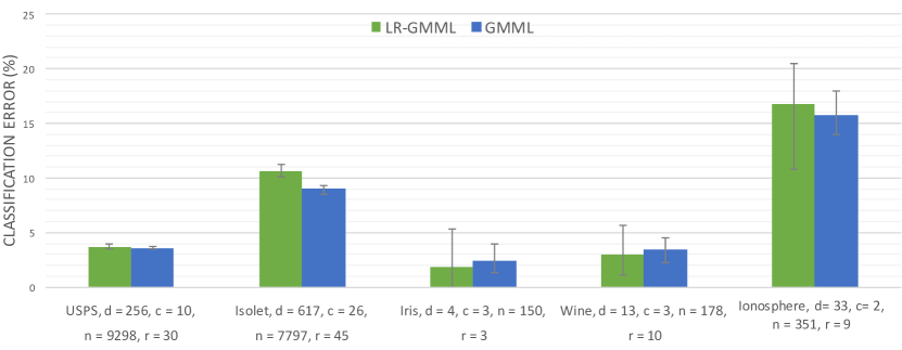
Figure 1: Classification error rates of k-NN classifier comparing LR-GMML with GMML. Dimensionality of feature space ($d$), number of classes ($c$), number of total data points ($n$), and the rank used in LR-GMML ($r$) are listed below each dataset.

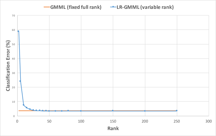
(a) USPS

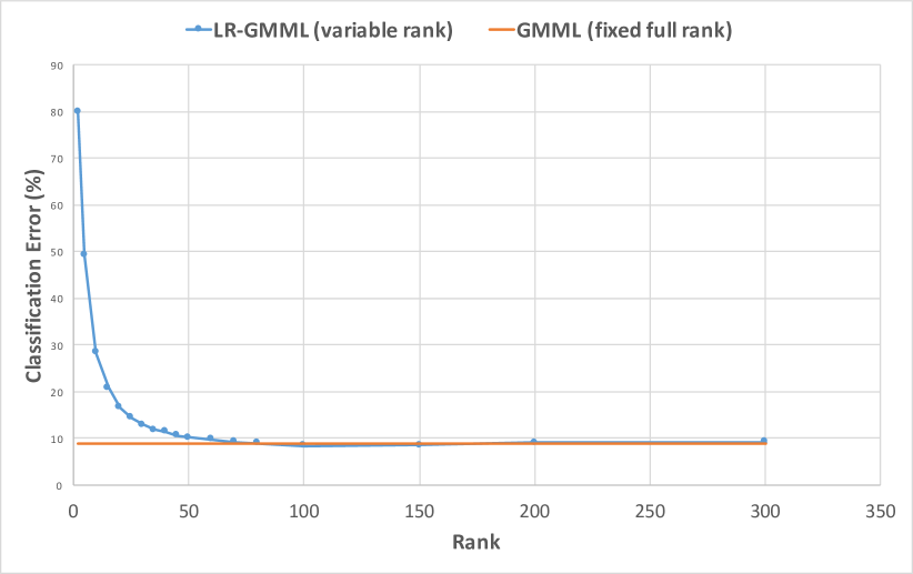
(b) Isolet

Figure 2: Classification error rates for LR-GMML for various low rank settings in comparison with that of GMML.

5 Conclusion

We presented a low-rank variant of the geometric mean metric learning (GMML) algorithm. The problem is shown to be an optimization problem on the Grassmann manifold, for which we exploit the Riemannian framework to develop a conjugate gradients solver. Our results show that even at lower-ranks, our low-rank variant LR-GMML performs as good as the full space (standard) GMML algorithm on many standard datasets. In future, we intend to work on larger datasets as well as in an online learning setting. Another direction is exploring LR-GMML with recently proposed deep learning techniques.

References

- Absil et al. (2008) Absil, P.-A., Mahoney, R., and Sepluchre, R. Optimization algorithms on matrix manifolds. Princeton University Press, 2008.
- Boumal et al. (2014) Boumal, N., Mishra, B., Absil, P.-A., and Sepulchre, R. Manopt, a matlab toolbox for optimization on manifolds. Journal of Machine Learning Research, 15:1455–1459, 2014.
- Davis et al. (2007) Davis, J. V., Kulis, B., Jain, P., Sra, S., and Dhillon, I. S. Information-theoretic metric learning. In International Conference on Machine Learning (ICML), pp. 209–216, 2007.
- Harandi et al. (2017) Harandi, M., Salzmann, M., and Hartley, R. Joint dimensionality reduction and metric learning: A geometric take. In International Conference on Machine Learning (ICML), pp. 1404–1413, 2017.
- Kulis (2012) Kulis, B. Metric learning: A survey. Foundations and Trends in Machine Learning, 5, 01 2012.
- Meyer et al. (2011) Meyer, G., Bonnabel, S., and Sepulchre, R. Regression on fixed-rank positive semidefinite matrices: a Riemannian approach. Journal of Machine Learning Research, 12:593–625, 2011.
- Weinberger & Saul (2009) Weinberger, K. Q. and Saul, L. K. Distance metric learning for large margin nearest neighbor classification. Journal of Machine Learning Research, 10:207–244, 2009.
- Zadeh et al. (2016) Zadeh, P. H., Hosseini, R., and Sra, S. Geometric mean metric learning. In International Conference on Machine Learning (ICML), pp. 2464–2471, 2016.