Charge-dependent Flow Induced by Magnetic and Electric Fields in Heavy Ion Collisions

Abstract

We investigate the charge-dependent flow induced by magnetic and electric fields in heavy ion collisions. We simulate the evolution of the expanding cooling droplet of strongly coupled plasma hydrodynamically, using the iEBE-VISHNU framework, and add the magnetic and electric fields as well as the electric currents they generate in a perturbative fashion. We confirm the previously reported effect of the electromagnetically induced currents Gursoy et al. (2014), that is a charge-odd directed flow $\Delta v_{1}$ that is odd in rapidity, noting that it is induced by magnetic fields (à la Faraday and Lorentz) and by electric fields (the Coulomb field from the charged spectators). In addition, we find a charge-odd $\Delta v_{3}$ that is also odd in rapidity and that has a similar physical origin. We furthermore show that the electric field produced by the net charge density of the plasma drives rapidity-even charge-dependent contributions to the radial flow $\langle p_{T}\rangle$ and the elliptic flow $\Delta v_{2}$. Although their magnitudes are comparable to the charge-odd $\Delta v_{1}$ and $\Delta v_{3}$, they have a different physical origin, namely the Coulomb forces within the plasma.

I Introduction

Large magnetic fields $\vec{B}$ are produced in all non-central heavy ion collisions (those with nonzero impact parameter) by the moving and positively charged spectator nucleons that “miss”, flying past each other rather than colliding, as well as by the nucleons that participate in the collision. Estimates obtained by applying the Biot-Savart law to collisions with an impact parameter $b=4$ fm yield $e|\vec{B}|/m_{\pi}^{2}\approx$ 1-3 about 0.1-0.2 fm$/c$ after a RHIC collision with $\sqrt{s}=200$ AGeV and $e|\vec{B}|/m_{\pi}^{2}\approx$ 10-15 at some even earlier time after an LHC collision with $\sqrt{s}=2.76$ ATeV Kharzeev et al. (2008); Skokov et al. (2009); Tuchin (2010); Voronyuk et al. (2011); Deng and Huang (2012); Tuchin (2013); McLerran and Skokov (2014); Gursoy et al. (2014). The interplay between these magnetic fields and quantum anomalies has been of much interest in recent years, as it has been predicted to lead to interesting phenomena including the chiral magnetic effect Kharzeev et al. (2008); Fukushima et al. (2008) and the chiral magnetic wave Kharzeev and Yee (2011); Burnier et al. (2011). This makes it imperative to establish that the presence of an early-time magnetic field can, via Faraday’s Law and the Lorentz force, have observable consequences on the motion of the final-state charged particles seen in the detectors Gursoy et al. (2014). Since the plasma produced in collisions of positively charged nuclei has a (small) net positive charge, electric effects – which is to say the Coulomb force – can also yield observable consequences to the motion of charged particles in the final state. These electric effects are distinct from the consequences of a magnetic field first studied in Ref. Gursoy et al. (2014), but comparable in magnitude. Our goal in this paper will be a qualitative, perhaps semi-quantitative, assessment of the observable effects of both magnetic and electric fields, arising just via the Maxwell equations and the Lorentz force law, so that experimental measurements can be used to constrain the strength of the fields and to establish baseline expectations against which to compare any other, possibly anomalous, experimental consequences of $\vec{B}$.

In previous work Gursoy et al. (2014) three of the authors noted that the magnetic field produced in a heavy ion collision could result in a measurable effect in the form of a charge-odd contribution to the directed flow coefficient $\Delta v_{1}$. This contribution has the opposite sign for positively vs. negatively charged hadrons in the final state and is odd in rapidity. However, the authors of Gursoy et al. (2014) neglected to observe that a part of this charge-odd, parity-odd effect originates from the Coulomb interaction. In particular it originates from the interaction between the positively charged spectators that have passed by the collision and the plasma produced in the collision, as will be explained in detail below.

The study in Ref. Gursoy et al. (2014) was simplified in many ways, including in particular by being built upon the azimuthally symmetric solution to the equations of relativistic viscous hydrodynamics constructed by Gubser in Ref. Gubser (2010). Because this solution is analytic, various practical simplifications in the calculations of Ref. Gursoy et al. (2014) followed. In reality magnetic fields do not arise in azimuthally symmetric collisions. The calculations of Ref. Gursoy et al. (2014) were intended to provide an initial order of magnitude estimate of the $\vec{B}$-driven, charge-odd, rapidity-odd contribution to $\Delta v_{1}$ in heavy ion collisions with a nonzero impact parameter, but the authors perturbed around an azimuthally symmetric hydrodynamic solution for simplicity. Also, the radial profile of the energy density in Gubser’s solution to hydrodynamics is not realistic. Here, we shall repeat and extend the calculation of Ref. Gursoy et al. (2014), this time building the perturbative calculation of the electromagnetic fields and the resulting currents upon numerical solutions to the equations of relativistic viscous hydrodynamics simulated within the iEBE-VISHNU framework Shen et al. (2016) that provide a good description of azimuthally anisotropic heavy ion collisions with a nonzero impact parameter.

The idea of Ref. Gursoy et al. (2014) is to calculate the electromagnetic fields, and then the incremental contribution to the velocity fields of the positively and negatively charged components of the hydrodynamic fluid (aka the electric currents) caused by the electromagnetic forces, in a perturbative manner. A similar conclusion have been reached in Roy et al. (2017) and Stewart and Tuchin (2018). One first computes the electric and magnetic fields $\vec{E}$ and $\vec{B}$ using the Maxwell equations as we describe further below. Then, at each point in the fluid, one transforms to the local fluid rest frame by boosting with the local background velocity field $\vec{v}_{\mathrm{flow}}$. Afterwards one computes the incremental drift velocity $\vec{v}_{\mathrm{drift}}$ caused by the electromagnetic forces in this frame by demanding that the electromagnetic force acting on a fluid unit cell with charge $q$ is balanced by the drag force. One then boosts back to the lab frame to obtain the total velocity field that now includes both $\vec{v}_{\mathrm{flow}}$ and $\vec{v}_{\mathrm{drift}}$, with $\vec{v}_{\mathrm{drift}}$ taking opposite signs for the positively and negatively charged components of the fluid. The authors of Ref. Gursoy et al. (2014) then use a standard Cooper-Frye freeze out analysis to show that the electromagnetic forces acting within the hydrodynamic fluid result in a contribution to the charge-odd directed flow parameter $\Delta v_{1}\equiv v_{1}(h^{+})-v_{1}(h^{-})$. We shall provide the (standard) definition of the directed flow $v_{1}$ in Section II. The charge-odd contribution $\Delta v_{1}$ is small but distinctive: in addition to being anti-symmetric under the flip of charge, it is also antisymmetric under flipping the rapidity. That the contribution has opposite sign for oppositely charged hadrons is easy to understand: it results from an electric current in the plasma. The fact that it has opposite sign at positive and negative rapidity can also easily be understood, as we explain in Fig. 1 and below.

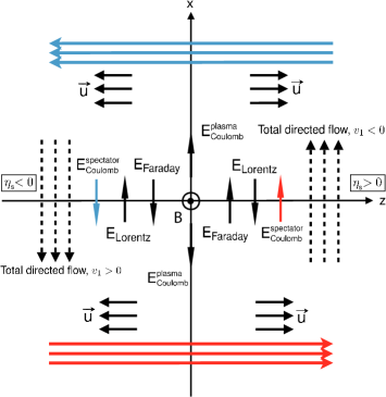
Figure 1: Schematic illustration of how the magnetic field $\vec{B}$ in a heavy ion collision results in a directed flow of electric charge, $\Delta v_{1}$. The collision occurs in the $z$-direction, meaning that the longitudinal expansion velocity $\vec{u}$ of the conducting QGP produced in the collision points in the $+z$ ($-z$) direction at positive (negative) $z$. We take the impact parameter vector to point in the $+x$ direction, choosing the nucleus moving toward positive (negative) $z$ to be located at negative (positive) $x$. The trajectories of the spectators that “miss” the collision because of the nonzero impact parameter are indicated by the red and blue arrows. This configuration generates a magnetic field $\vec{B}$ in the $+y$ direction, as shown. The directions of the electric fields (and hence currents) due to the Faraday, Lorentz and Coulomb effects are shown. The two different Coulomb contributions are indicated, one due to the force exerted by the spectators and the other coming from Coulomb forces within the plasma. The dashed arrows indicate the direction of the directed flow of positive charge in the case where the Faraday + spectator Coulomb effects are on balance stronger than the Lorentz effect. Hence, the total directed flow in this example corresponds to $v_{1}<0$ ($v_{1}>0$) for positive charges at spacetime rapidity $\eta_{s}>0$ ($\eta_{s}<0$), and opposite for negative charges.

As illustrated in Fig. 1, there are three distinct origins for a sideways push on charged components of the fluid, resulting in a sideways current:

1. Faraday: as the magnetic field decreases in time (see the right panel of Fig. 3 below), Faraday’s law dictates the induction of an electric field and, since the plasma includes mobile charges, an electric current. We denote this electric field by $\vec{E}_{F}$. Since $\vec{E}_{F}$ curls around the (decreasing) $\vec{B}$ that points in the $y$-direction, the sideways component of $E_{F}$ points in opposite directions at opposite rapidity, see Fig. 1.

2. Lorentz: since the hydrodynamic fluid exhibits a strong longitudinal flow velocity $\vec{v}_{\mathrm{flow}}$ denoted by $\vec{u}$ in Fig. 1, which points along the beam direction (hence perpendicular to $\vec{B}$), the Lorentz force exerts a sideways push on charged particles in opposite directions at opposite rapidity. Equivalently, upon boosting to the local fluid rest frame in which the fluid is not moving, the lab frame $\vec{B}$ yields a fluid frame $\vec{E}$ whose effects on the charged components of the fluid are equivalent to the effects of the Lorentz force in the lab frame. We denote this electric field by $\vec{E}_{L}$. Both $\vec{E}_{F}$ and $\vec{E}_{L}$ are of magnetic origin.

3. Coulomb: The positively charged spectators that have passed the collision zone exert an electric force on the charged plasma produced in the collision, which again points in opposite directions at opposite rapidity. We denote this electric field by $\vec{E}_{C}$. As we noted above, the authors of Ref. Gursoy et al. (2014) did not identify this contribution, even though it was correctly included in their numerical results.

As is clear from their physical origins, all three of these electric fields — and the consequent electric currents — have opposite directions at positive and negative rapidity. It is also clear from Fig. 1 that $\vec{E}_{F}$ and $\vec{E}_{C}$ have the same sign, while $\vec{E}_{L}$ opposes them. Hence, the sign of the total rapidity-odd, charge-odd, $\Delta v_{1}$ that results from the electric current driven by these electric fields depends on whether $\vec{E}_{F}+\vec{E}_{C}$ or $\vec{E}_{L}$ is dominant.

In this paper we make three significant advances relative to the exploratory study of Ref. Gursoy et al. (2014). First, as already noted we build our calculation upon a realistic hydrodynamic description of the expansion dynamics of the droplet of matter produced in a heavy ion collision with a nonzero impact parameter.

Second, we find that the same mechanism that produces the charge-odd $\Delta v_{1}$ also produces a similar charge-odd contribution to all the odd flow coefficients. The azimuthal asymmetry of the almond-shaped collision zone in a collision with nonzero impact parameter, its remaining symmetries under $x\leftrightarrow-x$ and $y\leftrightarrow-y$, and the orientation of the magnetic field $\vec{B}$ perpendicular to the beam and impact parameter directions together mean that the currents induced by the Faraday and Lorentz effects (illustrated in Fig. 1) make a charge-odd and rapidity-odd contribution to all the odd flow harmonics, not only to $\Delta v_{1}$. We compute the charge-odd contribution to $\Delta v_{3}$ in addition to $\Delta v_{1}$ in this paper.

Last but not least, we identify a new electromagnetic mechanism that generates another type of sideways current which generates a charge-odd, rapidity-even, contribution to the elliptical flow coefficient $\Delta v_{2}$. Although it differs in its symmetry from the three sources of sideways electric field above, it should be added to our list:

1. Plasma: As is apparent from the left panel of Fig. 2 in Section III and as we show explicitly in that Section, there is a non-vanishing outward-pointing component of the electric field already in the lab frame, because the plasma (and the spectators) have a net positive charge. We denote this component of the electric field by $\vec{E}_{P}$, since its origin includes Coulomb forces within the plasma.

At the collision energies that we consider, $\vec{E}_{P}$ receives contributions both from the spectator nucleons and from the charge density deposited in the plasma by the nucleons participating in the collision. As illustrated below by the results in the left panel of Fig. 2, the electric field will push an outward-directed current. As this field configuration is even in rapidity and odd under $x\leftrightarrow-x$ (which means that the radial component of the field is even under $x\leftrightarrow-x$), the current that it drives will yield a rapidity-even, charge-odd, contribution to the even flow harmonics, see Fig. 1. We shall demonstrate this by calculating the charge-dependent contribution to the radial flow, $\Delta\langle p_{T}\rangle$ (which can be thought of as $\Delta v_{0}$) and to the elliptic flow, $\Delta v_{2}$, that result from the electric field $\vec{E}_{P}$. Furthermore, we discover that these observables also receive a contribution from a component of the spectator-induced contribution to the electric field $\vec{E}_{F}+\vec{E}_{L}+\vec{E}_{C}$ that is odd under $x\leftrightarrow-x$ and even in rapidity.

In the next Section, we set up our model. In particular, we explain our calculation of the electromagnetic fields, the drift velocity and the freezeout procedure from which we read off the charge-dependent contributions to the radial $\langle p_{T}\rangle$ and to the anisotropic flow parameters $v_{1}$, $v_{2}$ and $v_{3}$. In Section III we present numerical results for the electromagnetic fields. Then in Section IV we move on to the calculation of the flow coefficients, for collisions with both RHIC and LHC energies, for pions and for protons, for varying centralities and ranges of $p_{T}$, and for several values of the electrical conductivity $\sigma$ of the plasma and the drag coefficient $\mu m$. The latter two being the properties of the plasma to which the effects that we analyse are sensitive. Finally in Section V we discuss the validity of the various approximations used in our calculations, discuss other related work, and present an outlook.

II Model Setup

We simulate the dynamical evolution of the medium produced in heavy-ion collisions using the iEBE-VISHNU framework described in full in Ref. Shen et al. (2016). We take event-averaged initial conditions from a Monte-Carlo-Glauber model, obtaining the initial energy density profiles by first aligning individual bumpy events with respect to their second-order participant plane angles (the appropriate proxy for the reaction plane in a bumpy event) and then averaging over 10,000 events. The second order participant plane of the averaged initial condition, $\Psi_{2}^{\mathrm{PP}}$, is rotated to align with the $x$-axis, which is to say we choose coordinates such that the averaged initial condition has $\Psi_{2}^{\mathrm{PP}}=0$ and an impact parameter vector that points in the $+x$ direction. The hydrodynamic calculation that follows assumes longitudinal boost-invariance and starts at $\tau_{0}=0.4$ fm/$c$. We then evolve the relativistic viscous hydrodynamic equations for a fluid with an equation of state based upon lattice QCD calculations, choosing the s95p-v1-PCE equation of state from Ref. Huovinen and Petreczky (2010) which implements partial chemical equilibrium at $T_{\mathrm{chem}}=150$ MeV. The kinetic freeze-out temperature is fixed to be 105 MeV to reproduce the mean $p_{T}$ of the identified hadrons in the final state. Specifying the equations of relativistic viscous hydrodynamics requires specifying the temperature dependent ratio of the shear viscosity to the entropy density, $\eta/s(T)$, in addition to specifying the equation of state. Following Ref. Niemi et al. (2011), we choose

$$\frac{\eta}{s}(T)=\left\{\begin{array}[]{rcl}\left(\frac{\eta}{s}\right)_{\mathrm{min}}+0.288\left(\frac{T}{T_{\mathrm{tr}}}-1\right)+0.0818\left(\left(\frac{T}{T_{\mathrm{tr}}}\right)^{2}-1\right)&\mbox{for}&T>T_{\mathrm{tr}}\\ \left(\frac{\eta}{s}\right)_{\mathrm{min}}+0.0594\left(1-\frac{T}{T_{\mathrm{tr}}}\right)+0.544\left(1-\left(\frac{T}{T_{\mathrm{tr}}}\right)^{2}\right)&\mbox{for}&T<T_{\mathrm{tr}}\end{array}\right..$$ (1)

We choose $(\eta/s)_{\mathrm{min}}=0.08$ at $T_{\mathrm{tr}}=180$ MeV. These choices result in hydrodynamic simulations that yield reasonable agreement with the experimental measurements over all centrality and collision energies, see for example Fig. 5 in Section IV below.

The electromagnetic fields are generated by both the spectators and participant charged nucleons. The transverse distribution of the right-going ($+$) and left-going ($-$) charge density profiles $\rho^{\pm}_{\mathrm{spectator}}(\vec{x}_{\perp})$ and $\rho^{\pm}_{\mathrm{participant}}(\vec{x}_{\perp})$ are generated by averaging over 10,000 events using the same Monte-Carlo-Glauber model used to initialize the hydrodynamic calculation. The external charge and current sources for the electromagnetic fields are then given by

$$\rho_{\mathrm{ext}}(\vec{x}_{\perp},\eta_{s})=\rho^{+}_{\mathrm{ext}}(\vec{x}_{\perp},\eta_{s})+\rho^{-}_{\mathrm{ext}}(\vec{x}_{\perp},\eta_{s})$$ (2)

$$\vec{J}_{\mathrm{ext}}(\vec{x}_{\perp},\eta_{s})=\vec{J}^{+}_{\mathrm{ext}}(\vec{x}_{\perp},\eta_{s})+\vec{J}^{-}_{\mathrm{ext}}(\vec{x}_{\perp},\eta_{s})$$ (3)

with

$$\rho^{\pm}_{\mathrm{ext}}(\vec{x}_{\perp},\eta_{s}) = \rho^{\pm}_{\mathrm{spectator}}(\vec{x}_{\perp})\delta(\eta_{s}\mp y_{\mathrm{beam}})+\rho^{\pm}_{\mathrm{participant}}(\vec{x}_{\perp})f^{\pm}(\eta_{s})$$ (4)

$$\vec{J}^{\pm}_{\mathrm{ext}}(\vec{x}_{\perp},\eta_{s}) = \vec{\beta}^{\pm}(\eta_{s})\rho^{\pm}_{\mathrm{ext}}(\vec{x}_{\perp},\eta_{s})\quad\mbox{with}\quad\vec{\beta}^{\pm}=(0,0,\pm\tanh(\eta_{s})).$$ (5)

Here we are making the Bjorken approximation: the space-time rapidities $\eta_{s}$ of the external charges are assumed equal to their rapidity. The spectators fly with the beam rapidity $y_{\mathrm{beam}}$ and the participant nucleons lose some rapidity in the collisions; their rapidity distribution in Eq. (4) is assumed to be Kharzeev (1996); Kharzeev et al. (2008); Gursoy et al. (2014)

$$f^{\pm}(y)=\frac{1}{4\sinh(y_{\mathrm{beam}}/2)}e^{\pm y/2}\quad\mbox{for}\quad-y_{\mathrm{beam}}<y<y_{\mathrm{beam}}.$$ (6)

The electromagnetic fields generated by the charges and currents evolve according to the Maxwell equations

$$(\nabla^{2}-\partial_{t}^{2}-\sigma\partial_{t})\vec{B} = -\vec{\nabla}\times\vec{J}_{\mathrm{ext}}$$ (7)

$$(\nabla^{2}-\partial_{t}^{2}-\sigma\partial_{t})\vec{E} = \frac{1}{\epsilon}\vec{\nabla}\rho_{\mathrm{ext}}+\partial_{t}\vec{J}_{\mathrm{ext}}\,.$$ (8)

Here $\sigma$ is the electrical conductivity of the QGP plasma. As in Ref. Gursoy et al. (2014), we shall make the significant simplifying assumption of treating $\sigma$ as if it were a constant. We make this assumption only because it permits us to use a semi-analytic form for the evolution of the electromagnetic fields rather than having to solve Eqs. (7) and (8) fully numerically. This simplification therefore significantly speeds up our calculations. In reality, $\sigma$ is certainly temperature dependent: just on dimensional grounds it is expected to be proportional to the temperature of the plasma, meaning that $\sigma$ should be a function of space and time as the plasma expands and flows hydrodynamically, with $\sigma$ decreasing as the plasma cools. Furthermore, during the pre-equilibrium epoch $\sigma$ should rapidly increase from zero to its equilibrium value. Taking all of this into consideration would require a full, numerical, magnetohydrodynamical analysis, something that we leave for the future. Throughout most of this paper, we shall follow Ref. Gursoy et al. (2014) and set the electrical conductivity to the constant value $\sigma=0.023$ fm^-1 which, according to the lattice QCD calculations in Refs. Ding et al. (2011); Francis and Kaczmarek (2012); Brandt et al. (2013); Amato et al. (2013); Kaczmarek and Muller (2014), corresponds to $\sigma$ in three-flavor quark-gluon plasma at $T\sim 250$ MeV. The numerical code that we have used to compute the evolution of the electromagnetic fields can be found at https://github.com/chunshen1987/Heavy-ion_EM_fields.

With the evolution of the electromagnetic fields in hand, the next step is to compute the drift velocity $\vec{v}_{\rm drift}$ that the electromagnetic field induces at each point on the freeze-out surface. Because this drift velocity is only a small perturbation compared to the background hydrodynamic flow velocity, $|\vec{v}_{\mathrm{drift}}|\ll|\vec{v}_{\mathrm{flow}}|$, we can obtain $\vec{v}_{\rm drift}$ by solving the force-balance equation Gursoy et al. (2014)

$$m\frac{d\vec{v}^{\mathrm{\,lrf}}_{\mathrm{drift}}}{dt}=q\vec{v}^{\mathrm{,\ lrf}}_{\mathrm{drift}}\times\vec{B}^{\mathrm{\,lrf}}+q\vec{E}^{\mathrm{\,lrf}}-\mu m\vec{v}^{\mathrm{\,lrf}}_{\mathrm{drift}}=0$$ (9)

in its non-relativistic form in the local rest frame of the fluid cell of interest. The last term in (9) describes the drag force on a fluid element with mass $m$ on which some external (in this case electromagnetic) force is being exerted, with $\mu$ the drag coefficient. The calculation of $\mu m$ for quark-gluon plasma in QCD remains an open question. In the ${\cal N}=4$ supersymmetric Yang-Mills (SYM) theory plasma it should be accessible via a holographic calculation. At present its value is known precisely only for heavy quarks in $\mathcal{N}=4$ SYM theory, in which Herzog et al. (2006); Casalderrey-Solana and Teaney (2006); Gubser (2006),

$$\mu m=\frac{\pi\sqrt{\lambda}}{2}T^{2}$$ (10)

with $\lambda\equiv g^{2}N_{c}$ the ’t-Hooft coupling, $g$ being the gauge coupling and $N_{c}$ the number of colors. For our purposes, throughout most of this paper we shall follow Ref. Gursoy et al. (2014) and use (9) with $\lambda=6\pi$. We investigate the consequences of varying this choice in Section IV.2. Finally, the drift velocity $\vec{v}^{\mathrm{\,lrf}}_{\mathrm{drift}}$ in every fluid cell along the freeze-out surface is boosted by the flow velocity to bring it back to the lab frame, $V^{\mu}=(\Lambda_{\mathrm{flow}})^{\mu}\,_{\nu}(u^{\mathrm{lrf}}_{\mathrm{drift}})^{\nu}$, where $(\Lambda_{\mathrm{flow}})^{\mu}\,_{\nu}$ is the Lorentz boost matrix associated with the hydrodynamic flow velocity $u^{\mu}_{\mathrm{flow}}$.

With the full, charge-dependent, fluid velocity $V^{\mu}$ — including the sum of the flow velocity and the charge-dependent drift velocity induced by the electromagnetic fields — in hand, we now use the Cooper-Frye formula Cooper and Frye (1974),

$$\frac{dN}{dyp_{T}dp_{T}d\phi}=\frac{g}{(2\pi)^{3}}\int_{\Sigma}p^{\mu}d\sigma_{\mu}\left[f_{0}+f_{0}(1\mp f_{0})\frac{p^{\mu}p^{\nu}\pi_{\mu\nu}}{2T^{2}(e+P)}\right]$$ (11)

to integrate over the freezeout surface (the spacetime surface at which the matter produced in the collision cools to the freezeout temperature that we take to be 105 MeV) and obtain the momentum distribution for hadrons with different charges. Here, $g$ is the hadron’s spin degeneracy factor and the equilibrium distribution function is given by

$$f_{0}=\frac{1}{\exp((p\cdot V)/T)\pm 1}.$$ (12)

With the momentum distribution for hadrons with different charge in hand, the final step in the calculation is the evaluation of the anisotropic flow coefficients as function of rapidity:

$$v_{n}(y)\equiv\frac{\int dp_{T}d\phi\,p_{T}\frac{dN}{dyp_{T}dp_{T}d\phi}\cos\left[n(\phi-\Psi_{n})\right]}{\int dp_{T}d\phi\,p_{T}\frac{dN}{dyp_{T}dp_{T}d\phi}}$$ (13)

where $\Psi_{n}=0$ is the event-plane angle in the numerical simulations. In order to define the sign of the rapidity-odd directed flow $v_{1}$, we choose the spectators at positive $x$ to fly toward negative $z$, as illustrated in Fig. 1. We can then compute the odd component of $v_{1}(y)$ according to

$$v_{1}^{\mathrm{odd}}=\frac{1}{2}(v_{1}(\Psi_{+})-v_{1}(\Psi_{-})),$$ (14)

Experimentally, the rapidity-odd directed flow $v_{1}^{\mathrm{odd}}$ is measured Margutti (2017) by correlating the directed flow vector of particles of interest, ${\bf Q}^{\mathrm{POI}}_{1}=\sum_{j=1}^{M^{\mathrm{POI}}}e^{i\phi_{j}}$, with the flow vectors from the energy deposition of spectators in the zero-degree calorimeter (ZDC), ${\bf Q}^{\mathrm{ZDC}}_{\pm}=\sum_{j}E^{\pm}_{j}r_{j}e^{i\phi_{j}}$. The directed flow is defined using the scalar-product method:

$$v_{1}(\Psi_{\pm})=\frac{1}{\langle M^{\mathrm{POI}}\rangle_{\mathrm{ev}}}\frac{\langle{\bf Q}^{\mathrm{POI}}_{1}\cdot({\bf Q}^{\mathrm{ZDC}}_{\pm})^{*}\rangle_{\mathrm{ev}}}{\sqrt{\langle|{\bf Q}^{\mathrm{ZDC}}_{+}\cdot({\bf Q}^{\mathrm{ZDC}}_{-})^{*}|\rangle_{\mathrm{ev}}}}\ .$$ (15)

In the definition of ${\bf Q}^{\mathrm{ZDC}}_{\pm}$, the index $j$ runs over all the segments in the ZDC and $E_{j}$ denotes the energy deposition at ${\bf x}_{j}=r_{j}e^{i\phi_{j}}$. In our notation, the flow vector angle $\Psi_{+}=\pi$ in the forward ($+z$ direction) ZDC and $\Psi_{-}=0$ in the backward ($-z$) direction ZDC. The odd component of $v_{1}(y)$ that we compute according to Eqs. (13) and (14) can be directly compared to $v_{1}^{\rm odd}$ defined from the experimental definition of $v_{1}(\Psi_{\pm})$ in (15).

In order to isolate the small contribution to the various flow observables that was induced by the electromagnetic fields, separating it from the much larger background hydrodynamic flow, we compute the difference between the value of a given flow observable for positively and negatively charged hadrons:

$$\Delta\langle p_{T}\rangle\equiv\langle p_{T}\rangle(h^{+})-\langle p_{T}\rangle(h^{-})$$ (16)

and

$$\Delta v_{n}\equiv v_{n}(h^{+})-v_{n}(h^{-}),$$ (17)

are the quantities of interest.

III Electromagnetic fields

It is instructive to analyze the spatial distribution and the evolution of the electromagnetic fields in heavy-ion collisions. We shall do so in this Section, before turning to a discussion of the results of our calculations in the next Section.

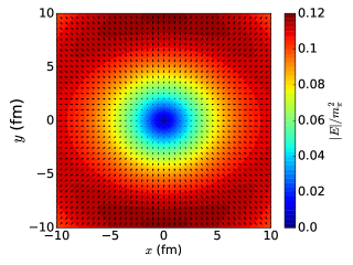
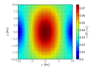
Figure 2: The electric (left) and magnetic (right) fields in the transverse plane at $z=0$ in the lab frame at a proper time $\tau=1$ fm/c after a Pb+Pb collision with 20-30% centrality (corresponding to impact parameters in the range 6.24 fm $<b<$ 9.05 fm) and with a collision energy $\sqrt{s}=2.76$ ATeV. The fields are produced by the spectator ions moving in the $+z$ ($-z$) direction for $x<0$ ($x>0$) as well as by the ions that participate in the collision. In both panels, the contribution from the spectators is larger, however. The direction of the fields are shown by the black arrows. The strength of the field is indicated both by the length of the arrows and by the color. We see that the magnetic field is strongest at the center of the plasma, where it points in the $+y$ direction as anticipated in Fig. 1. The electric field points in a generally outward direction and is strongest on the periphery of the plasma. Its magnitude is not azimuthally symmetric: the field is on average stronger where it is pointing in the $\pm y$ directions than where it is pointing in the $\pm x$ directions.

Fig. 2 presents our calculation of the magnitude and direction of the electromagnetic fields, both electric and magnetic, in the lab frame across the $z=0$ transverse plane at a proper time $\tau=1$fm/c after a Pb+Pb collision with 20-30% centrality and a collision energy of $\sqrt{s}=2.76$ ATeV. These electric and magnetic fields are produced by both spectator and participant ions in the two incoming nuclei. We outlined the calculation in Section II; it follows Ref. Gursoy et al. (2014). The spectator nucleons give the dominant contributions to the $\vec{B}$ field. The beam directions for the ions at $x>0$ ($x<0$) are chosen as $-z$ ($+z$), as in Fig. 1.

The left panel in Fig. 2 includes three of the four different components of the electric field that we discussed in the Introduction, namely the electric field generated by Faraday’s law $\vec{E}_{F}$, the Coulomb field sourced by the spectators $\vec{E}_{C}$, and the Coulomb field sourced by the net charge in the plasma $\vec{E}_{P}$. Their sum gives the total electric field in the lab frame, which is what is plotted. When we transform to the local rest frame of a moving fluid cell, namely the frame in which we calculate the electromagnetically induced drift velocity of positive and negative charges in that fluid cell, there is an additional component originating from the Lorentz force law, $\vec{E}_{L}$, as explained in the Introduction. The total electric field in the rest frame, which now also includes the $E_{L}$ component, is shown below in the left panel of Fig. 4 as a function of time.

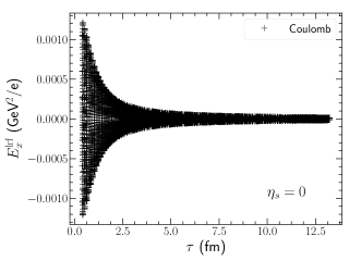
Figure 3: Left: The $x$-component of the electric field in the local fluid rest frame at points on the freezeout surface at spacetime rapidity $\eta_{s}=0$, as a function of proper time. Each cross corresponds to a single fluid cell on the freezeout surface, with the vertical line of crosses at any single $\tau$ corresponding to different points on the freezeout surface at that $\tau$. Only the Coulomb electric field generated by the net charge in the plasma contributes at $\eta_{s}=0$, and by symmetry there for every point where $E_{x}^{\,\rm lrf}>0$ there is a point where $E_{x}^{\,\rm lrf}<0$. Right: Time dependence of the $y$-component of the magnetic field in the lab frame at $\eta_{s}=0$. Again, each cross corresponds to a single point on the freeze-out surface. We see that $B_{y}>0$ as diagrammed in Fig. 1 and shown in Fig. 2, and here we can see how $B_{y}$ decreases with time.

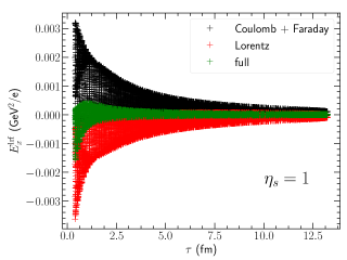
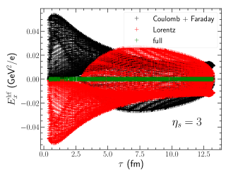
Figure 4: Contributions to the electric field in the local rest frame of a unit cell in the fluid on the freezeout surface at a specified, non-vanishing, spacetime rapidity $\eta_{s}$: $\eta_{s}=1$ in the left panel and $\eta_{s}=3$ in the right panel. Each unit cell is represented in the figure by a black cross, a red cross, and a green cross. Black crosses denote the contribution to the electric field at a given fluid cell in its local rest frame coming from the Coulomb and Faraday effects. Red crosses denote the contribution from the Lorentz force. And, green crosses represent the total electric field at the fluid cell, namely the sum of a black cross and a red cross. We observe that the Coulomb+Faraday and Lorentz contributions to the electric field point in opposite directions, as sketched in Fig. 1, and furthermore see that the two contributions almost cancel at large $\eta_{s}$, as we shall discuss in Section IV.1. We shall see there that the Coulomb+Faraday contribution is slightly larger in magnitude than the Lorentz contribution.

The magnetic field in the right panel of Fig. 2 indeed decays as a function of time as shown in the right panel of Fig. 3. Via Faraday’s law this induces a current in the same direction as the current pushed by the Coulomb electric field coming from the spectators, and it opposes the current caused by the Lorentz force on fluid elements moving in the longitudinal direction, as sketched in Fig. 1 and seen in Fig. 4.

When solving the force-balance equation, Eq. (9), we find that the drift velocity is mainly determined by the electric field in the local local fluid rest frame. To understand how the Coulomb, Lorentz and Faraday effects contribute to the drift velocity on the freeze-out surface it is instructive to study how the different effects contribute to the electric field in the local fluid rest frame. We do so at $\eta_{s}=0$ in the left panel of Fig. 3. At $\eta_{s}=0$, only the Coulomb effect contributes. This means that when in Section IV we compute the charge-odd contribution to the even flow harmonics at $\eta_{s}=0$ this will provide an estimate of the magnitude of the Coulomb contribution to the flow coefficients. In Fig. 4 we look at the different contributions to the electric field in the local fluid rest frame at $\eta_{s}=1$ and $\eta_{s}=3$. We see that the Coulomb + Faraday and Lorentz effects point in opposite directions, and almost cancel at large spacetime rapidity. We discuss the origin and consequences of this cancellation in Section IV.1 below.

IV Results

In this Section we present our results for the charge-dependent contributions to the anisotropic flow induced by the electromagnetic effects introduced in Section I. As we have described in Section II, to obtain the anisotropic flow coefficients we input the electromagnetic fields in the local rest frame of the fluid, calculated in Section III, into the force-balance equation (9) which then yields the electromagnetically induced component of the velocity field of the fluid. This velocity field is then input into the Cooper-Frye freezout procedure Cooper and Frye (1974) to obtain the distribution of particles in the final state and, in particular, the anisotropic flow coefficients Gursoy et al. (2014).

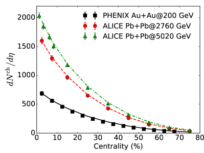
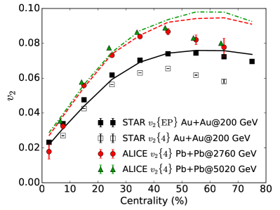
Figure 5: To get a sense of how well the solution to relativistic viscous hydrodynamics upon which we build our calculation of electromagnetic fields and currents describes heavy ion collisions, we compare our results for charged hadron multiplicities (left) and elliptic flow coefficients (right) to experimental measurements at the top RHIC and LHC energies from Refs. Adler et al. (2005); Aamodt et al. (2011); Adam et al. (2016a) and Refs. Adams et al. (2005); Aamodt et al. (2010); Adam et al. (2016b), respectively.

To provide a realistic dynamical background on top of which to compute the electromagnetic fields and consequent currents, we have calibrated the solutions to relativistic viscous hydrodynamics that we use by comparing them to experimental measurements of hadronic observables. To give a sense of the agreement that we have obtained, in Fig. 5 we show our results for the centrality dependences of charged hadron multiplicity and elliptic flow coefficients are shown for heavy-ion collisions at three collision energies as well as data from STAR, PHENIX and ALICE Collaborations Adler et al. (2005); Aamodt et al. (2011); Adam et al. (2016a); Adams et al. (2005); Aamodt et al. (2010); Adam et al. (2016b). Since we do not have event-by-event fluctuations in our calculations, we compare our results for the elliptic flow coefficent $v_{2}$ to experimental measurements of $v_{2}$ from the 4-particle cumulant, $v_{2}\{4\}$ Qiu and Heinz (2011). With the choice of the specific shear viscosity $\eta/s(T)$ that we have made in Eq. (1), our model provides a reasonable agreement with charged hadron $v_{2}\{4\}$ for heavy ion collisions with centralities up to the 40-50% bin.

To isolate the effect of electromagnetic fields on charged hadron flow observables, we study the difference between the $v_{n}$ of positively charged particles and the $v_{n}$ of negatively charged particles as defined in Eq. (17). We also study the difference between the mean transverse momentum $\langle p_{T}\rangle$ of positively charged hadrons and that of negatively charged hadrons. This provides us with information about the modification in the hydrodynamic radial flow induced by the electromagnetic fields. The difference between the charge-dependent flow of light pions and heavy protons is also compared. Hadrons with different masses have different sensitivities to the underlying hydrodynamic flow and to the electromagnetic fields.

We should distinguish the charge-odd contributions to the odd flow moments, $\Delta v_{1}$, $\Delta v_{3}$, $\ldots$, from the charge-dependent contributions to the even ones, $\Delta v_{2}$, $\Delta v_{4}$, $\ldots$, as they have qualitatively different origins. The charge-odd contributions to the odd flow coefficients induced by electromagnetic fields, $\Delta v_{2n-1}$, are rapidity-odd: $\Delta v_{2n-1}(\eta_{s})=-\Delta v_{2n-1}(-\eta_{s})$. This can easily be understood by inspecting Fig. 1, where we describe different effects that contribute to the total the electric field in the plasma. This can also be proven analytically by studying the transformation property of $\Delta v_{n}$ under $\eta\to-\eta$. As we have seen in Section I, there are three basic effects that contribute. First, there is the electric field produced directly by the positively charged spectator ions. They generate electric fields in opposite directions in the $z>0$ and $z<0$ regions. We call this the Coulomb electric field $\vec{E}_{C}$, as the resulting electric current in the plasma is a direct result of the Coulomb force between the spectators and charges in the plasma. Then there are the two separate magnetically induced electric fields, as discussed in Ref. Gursoy et al. (2014). The Faraday electric field $\vec{E}_{F}$ results from the rapidly decreasing magnitude of the magnetic field perpendicular to the reaction plane, see Fig. 1, as a consequence of Faraday’s law. Note that $\vec{E}_{F}$ and $\vec{E}_{C}$ point in the same directions. Finally, there is another magnetically induced electric field, the Lorentz electric field $\vec{E}_{L}$ that can be described in the lab frame as the Lorentz force on charges that are moving because of the longitudinal expansion of the plasma and that are in a magnetic field. Upon transforming to the local fluid rest frame, the lab-frame magnetic field becomes an electric field that we denote $\vec{E}_{L}$. As shown in Fig. 1, $\vec{E}_{L}$ points in the opposite direction to $\vec{E}_{F}$ and $\vec{E}_{C}$.

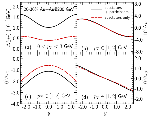
Figure 6: The solid black curves display the principal results of our calculations for 20-30% centrality Au+Au collisions at 200 GeV, as at RHIC. We show the contribution to the mean-$p_{T}$ of charged pions and the first three $v_{n}$ coefficients induced by the electromagnetic fields that we have calculated, isolating the electromagnetically induced effects by taking the difference between the calculated value of each observable for $\pi^{+}$ and $\pi^{-}$ mesons, namely the charge-odd or charge-dependent contributions that we denote $\Delta\langle p_{T}\rangle$ and $\Delta v_{n}$. We see rapidity-odd contributions $\Delta v_{1}$ and $\Delta v_{3}$ and rapidity-even contributions $\Delta\langle p_{T}\rangle$ and $\Delta v_{2}$. The red dashed curves show the results we obtain when we calculate the same observables in the presence of the electromagnetic fields produced by the spectators only. We see that the dominant contribution to the odd $v_{n}$’s is generated by these spectator-induced fields, whereas the even $v_{n}$’s also receive a significant contribution from the Coulomb force exerted on charges in the plasma by other charges in the plasma, originating from the participant nucleons.

On the other hand, the charge-dependent contributions to the even order anisotropic flow coefficients $v_{2n}$ are even under $\eta_{s}\to-\eta_{s}$. Obviously this cannot arise from the rapidity-odd electric fields described above. Instead, we find that although the electromagnetic contribution to the $v_{2n}$ receives some contribution from components of the electric fields above that are rapidity-even and that are odd under $x\rightarrow-x$, it also receives an important contribution from the Coulomb force between the net positive electric charge in the plasma. This arises as a result of the Coulomb force exerted on the charges in the plasma by each other — as opposed to the Coulomb force exerted on charges in the plasma by the spectator ions. This electric field is non-trivial even at $z=0$ as shown in Fig. 2 (left). We call this field the plasma electric field and denote it by $\vec{E}_{P}$. This contributes to the net $\Delta v_{2}$ and it is clear from the geometry that it makes no contribution to the odd flow harmonics.

In Fig. 6, we begin the presentation of our principal results. This figure shows $\Delta v_{n}$, the charge-odd contribution to the anisotropic flow harmonics induced by electromagnetic fields, for pions in 20-30% Au+Au collisions at 200 GeV. It also shows the difference in the mean-$p_{T}$ of particles with positive and negative charge, which shows how the electromagnetic fields modify the hydrodynamic radial flow. The radial outward pointing electric fields in Fig. 2 increase the radial flow for positively charged hadrons while reducing the flow for negative particles. We see that the effect is even in rapidity. Fig. 6 shows that these fields also make a charge-odd, rapidity-even contribution to $v_{2}$.

We compare the red dashed curves, arising from electromagnetic effects by spectators only, with the solid black curves that show the full calculation including the participants. Noting that the lines are significantly different it follows that the Coulomb force exerted on charges in the plasma by charges in the plasma makes a large contribution to $\Delta\langle p_{T}\rangle$ and $\Delta v_{2}$. The induced $\Delta\langle p_{T}\rangle$ is larger at forward and backward rapidities, because the electric fields from the spectators and from the charge density in the plasma deposited according to the distribution (6) are both stronger there.

The electromagnetically induced elliptic flow $\Delta v_{2}$ originates from the Coulomb electric field in the transverse plane, depicted in Fig. 2. We see there that the Coulomb field is stronger along the $y$-direction than in the $x$-direction. This reduces the elliptic flow $v_{2}$ for positively charged hadrons and increases it for negatively charged hadrons. Hence, $\Delta v_{2}$ is negative.

Note that $\Delta\langle p_{T}\rangle$ and $\Delta v_{2}$ are much smaller than $\langle p_{T}\rangle$ and $v_{2}$; in the calculation of Fig. 6, $\langle p_{T}\rangle\approx 0.47$ GeV and $v_{2}\approx 0.048$ for both the $\pi^{+}$ and $\pi^{-}$. The differences between these observables for $\pi^{+}$ and $\pi^{-}$ that we plot are much smaller, with $\Delta\langle p_{T}\rangle$ smaller than $\langle p_{T}\rangle$ by a factor of $\mathcal{O}(10^{-3})$ and $\Delta v_{2}$ smaller than $v_{2}$ by a factor of $\mathcal{O}(10^{-2})$ in Au+Au collisions at 200 GeV. This reflects, and is consistent with, the fact that the drift velocity induced by the electromagnetic fields is a small perturbation compared to the overall hydrodynamic flow on the freeze-out surface.

The electromagnetically induced contributions to the odd flow harmonics $\Delta v_{1}$ and $\Delta v_{3}$ are odd in rapidity. In our calculation, which neglects fluctuations, $v_{1}$ and $v_{3}$ both vanish in the absence of electromagnetic effects. We see from Fig. 6 that the magnitudes of $\Delta v_{1}$ and $\Delta v_{3}$ are controlled by the electromagnetic fields due to the spectators, namely $\vec{E}_{F}$, $\vec{E}_{C}$ and $\vec{E}_{L}$. By comparing the sign of the rapidity-odd $\Delta v_{1}$ that we have calculated in Fig. 6 to the illustration in Fig. 1, we see that the rapidity-odd electric current flows in the direction of $\vec{E}_{F}$ and $\vec{E}_{C}$, opposite to the direction of $\vec{E}_{L}$, meaning that $|\vec{E}_{F}+\vec{E}_{C}|$ is greater than $|\vec{E}_{L}|$. Our results for $\Delta v_{1}$ are qualitatively similar to those found in Ref. Gursoy et al. (2014), although they differ quantitatively because of the differences between our realistic hydrodynamic background and the simplified hydrodynamic solution used in Ref. Gursoy et al. (2014). Here, we find a nonzero $\Delta v_{3}$ in addition, also odd in rapidity, and with the same sign as $\Delta v_{1}$ and a similar magnitude. This is natural since $\Delta v_{3}$ receives a contribution from the mode coupling between the electromagnetically induced $\Delta v_{1}$ and the background elliptic flow $v_{2}$.

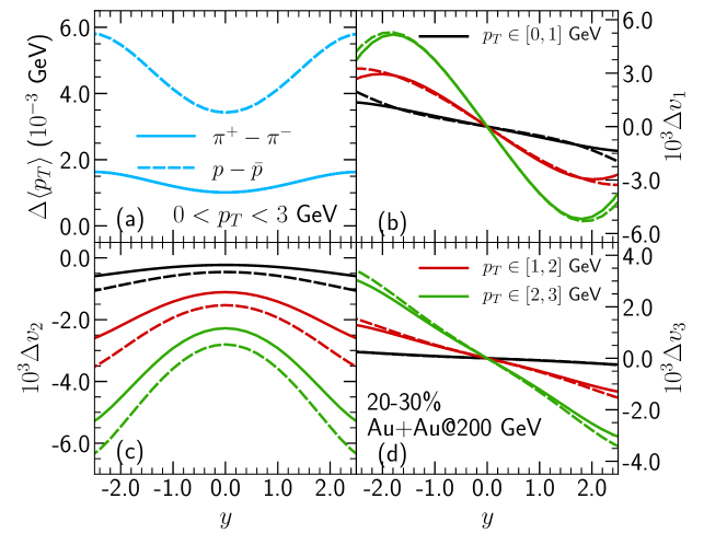
Figure 7: The electromagnetically induced difference between the mean $p_{T}$ and $v_{n}$ coefficients of $\pi^{+}$ and $\pi^{-}$ mesons (solid lines) and between protons and antiprotons (dashed lines) as a function of particle rapidity for 20-30% Au+Au collisions at 200 GeV. Three different $p_{T}$ integration ranges are shown for each of the $\Delta v_{n}$ as a function of particle rapidity.

In Fig. 7 we see that the heavier protons have a larger electromagnetically induced shift in their mean $p_{T}$ compared to that for the lighter pions. Because a proton has a larger mass than a pion, its velocity is slower than that of a pion with the same transverse momentum, $p_{T}$. Thus, when we compare pions and protons with the same $p_{T}$, the hydrodynamic radial flow generates a stronger blue shift effect for the less relativistic proton spectra, which is to say that the proton spectra are more sensitive to the hydrodynamic radial flow Heinz (2004). Similarly, when the electromagnetic fields that we compute induce a small difference between the radial flow velocity of positively charged particles relative to that of negatively charged particles, the resulting difference between the mean $p_{T}$ of protons and antiprotons is greater than the difference between the mean $p_{T}$ of positive and negative pions. Turning to the $\Delta v_{n}$’s, we see in Fig. 7 that the difference between the electromagnetically induced $\Delta v_{n}$’s for protons and those for pions are much smaller in magnitude. We shall also see below that these differences are modified somewhat by contributions from pions and protons produced after freezeout by the decay of resonances. For both these reasons, these differences cannot be interpreted via a simple blue shift argument. Fig. 7 also shows the charge-odd electromagnetically induced flow coefficients $\Delta v_{n}$ computed from charged pions and protons+antiprotons in three different $p_{T}$ ranges. The $\Delta v_{1}$, $\Delta v_{2}$ and $\Delta v_{3}$ all increase as the $p_{T}$ range increases, in much the same way that the background $v_{2}$ does. In the case of $\Delta v_{1}$, this agrees with what was found in Ref. Gursoy et al. (2014).

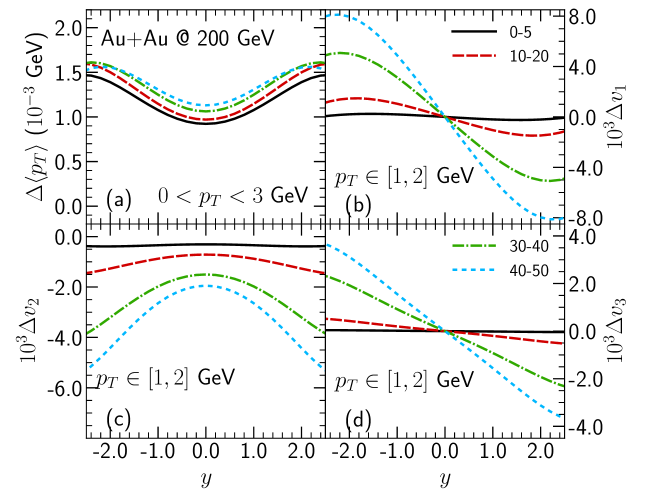
Figure 8: The centrality dependence of the electromagnetically induced flow difference in $\pi^{+}$ vs $\pi^{-}$ as a function of particle rapidity in Au+Au collisions at 200 GeV.

In Fig. 8 we study the centrality dependence of the electromagnetically induced flow in Au+Au collisions at 200 GeV. The difference between the flow of positive and negative pions, both the radial flow and the flow anisotropy coefficients, increases as one goes from central toward peripheral heavy ion collisions. However, the increase in $\Delta\langle p_{T}\rangle$ and $\Delta v_{2}$ is smaller than the increase in the odd $\Delta v_{n}$’s. This further confirms that the odd $\Delta v_{n}$’s are induced by the electromagnetic fields produced by the spectator nucleons only – since the more peripheral a collision is the more spectators there are.

Compared to any of the anisotropic flow coefficients $\Delta v_{n}$, the $\Delta\langle p_{T}\rangle$ shows the least centrality dependence because, as we saw in Fig. 6, $\Delta\langle p_{T}\rangle$ originates largely from the Coulomb field of the plasma, coming from the charge of the participants, with only a small contribution from the spectators. The increase of $\Delta v_{2}$ with centrality is intermediate in magnitude, since it originates both from the participants and from the spectators, as seen in Fig. 6. Another origin for the increase in electromagnetically induced effects in more peripheral collisions is that the typical lifetime of the fireball in these collisions is shorter compared to that in central collisions. This gives less time for the electromagnetic fields to decay by the time of peak particle production in more peripheral collisions. In the case of $\Delta\langle p_{T}\rangle$, which is dominantly controlled by the plasma Coulomb field which is less in more peripheral collisions where there is less plasma, this effect partially cancels the effect of the reduction in the fireball lifetime, and results in $\Delta\langle p_{T}\rangle$ being almost centrality independent.

Figure 9: The centrality dependence of the electromagnetically induced differences in the radial flow and anisotropic flow coefficients for positively and negatively charged hadrons, here at a fixed rapidity $y=-1$.

Fig. 9 further shows the centrality dependence of the electromagnetically induced difference between flow observables for positive and negative particles at a fixed rapidity. We observe that $\Delta\langle p_{T}\rangle$ does not vanish in central collisions. This further confirms that it is largely driven by the Coulomb field created by a net positive charge density in the plasma itself, as this Coulomb field is present in collisions with zero impact parameter whereas all spectator-induced effects vanish when there are no spectators. This charge density creates an outward electric field that generates an outward flux of positive charge in the plasma and leads to a non-vanishing charge-identified radial flow.

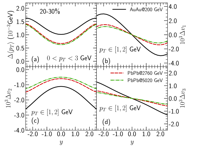
Figure 10: The collision energy dependence of the electromagnetically induced charge-odd contributions to flow observables. The difference of particle mean $p_{T}$ and $v_{n}$ between $\pi^{+}$ and $\pi^{-}$ are plotted as a function of particle rapidity for collisions at the top RHIC energy of 200 GeV and at two LHC collision energies.

In Fig. 10, we study the collision energy dependence of the effects of electromagnetic fields on charged hadron flow. The electromagnetically induced effects on the differences between flow observables for positive and negative particles are larger at the top RHIC energy than at LHC energies. This can be understood as arising from the fact that because the spectators pass by more quickly in higher energy collisions the spectator-induced electromagnetic fields decrease more rapidly with time in LHC collisions than in RHIC collisions. Furthermore, in higher energy collisions at the LHC the fireball lives longer, further reducing the magnitude of the electromagnetic fields on the freeze-out surface. The results illustrated in Fig. 10 motivate repeating our analysis for the lower energy collisions being done in the RHIC Beam Energy Scan, although doing so will require more sophisticated underlying hydrodynamic calculations and we also note that in such collisions there are other physical effects that contribute significantly to $\Delta\langle p_{T}\rangle$ and $\Delta v_{2}$ Xu et al. (2012); Steinheimer et al. (2012); Ko et al. (2014); Adamczyk et al. (2013); Xu et al. (2014); Adamczyk et al. (2016); Xu and Ko (2016), in the case of $\Delta v_{2}$ for protons making a contribution with opposite sign to the one that we have calculated. For both these reasons, we leave such investigations to future work.

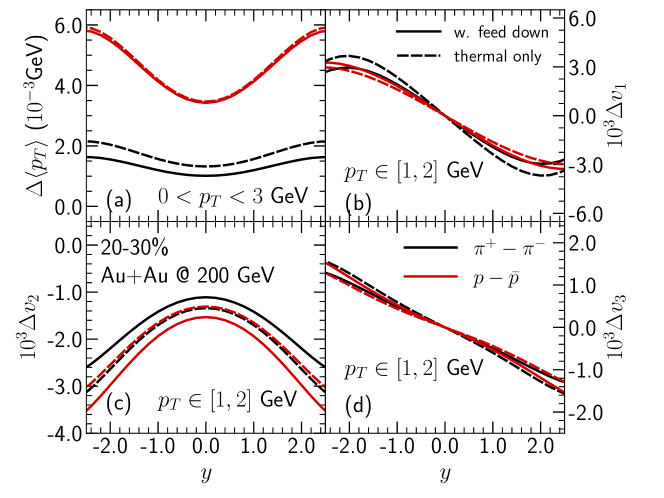
Figure 11: The solid curves include the contributions to the electromagnetically induced charge-dependent flow observables of pions and protons produced after freeze-out by resonance decay, often referred to as resonance feed-down contributions. In the dashed curves, pions and protons produced from resonance feed-down are left out.

Finally, in Fig. 11, we investigate the contribution of resonance decays to the electromagnetically induced charge-dependent contributions to flow observables that we have computed. These contributions are included in all our calculations with the exception of those shown as the dashed lines in Fig. 11, where we include only the hadrons produced directly at freezeout, leaving out those produced later as resonances decay. We see that the feed-down contribution from resonance decays does not significantly dilute the effects we are interested in. To the contrary, the magnitudes of the $\Delta v_{n}$ for protons are slightly increased by feed-down effects, in particular the significant contribution to the final proton yield coming from the decay of the $\Delta^{++}$ Qiu et al. (2012). Because the $\Delta^{++}$ resonance carries 2 units of the charge, its electromagnetically induced drift velocity is larger than those of protons.

This concludes the presentation of our central results. In the remainder of this Section, in two subsections we shall present a qualitative argument for why $\Delta v_{1}$ is as small as it is, and then take a brief look at how our results depend on the value of two important material properties of the plasma, namely the drag coefficient and the electrical conductivity.

IV.1 A qualitative argument for the smallness of $\Delta v_{1}$

As we have seen, the net effect on $\Delta v_{1}$ of the various contributions to the electric field turns out to be rather small in magnitude. This is because even though the contributions $\vec{E}_{C}+\vec{E}_{F}$ and $\vec{E}_{L}$ with opposite sign, shown separately in Fig. 4, are each relatively large in magnitude they cancel each other almost precisely. This leaves only a small net contribution that generates the charge-odd contributions to the odd flow harmonics that we have computed, $\Delta v_{1}$ and $\Delta v_{3}$. We see in Fig. 4 that this cancellation becomes more and more complete at larger $\eta_{s}$. In this subsection we provide a qualitative argument for this near-cancellation and explain why the cancellation becomes more complete at larger $\eta_{s}$.

One can find an expression for the total Faraday+Coulomb electric field $\vec{E}_{F+C}\equiv\vec{E}_{F}+\vec{E}_{C}$ by solving the Maxwell equations sourced by the spectator (and participant) charges. In general this determines both the electric and the magnetic fields in terms of the sources. However, we only need to express $\vec{E}_{F+C}$ in terms of $\vec{B}$ for the argument. In particular, we are interested in the $x$ component of this field as shown in Fig. 1. This is given by solving Faraday’s law $\nabla\times\vec{E}_{F+C}=-\partial\vec{B}/\partial t$ to obtain $E_{F+C,x}=B_{y}\coth(Y_{0}-\eta_{s})$, where $Y_{0}$ is the rapidity of the beam and $\eta_{s}$ is the spacetime rapidity. Since for both RHIC and LHC we have $Y_{0}\gg\eta_{s}$, one can safely ignore the $\eta_{s}$-dependence everywhere in the plasma, finding $E_{F+C,x}\approx B_{y}\coth(Y_{0})$. For the same reason, as $Y_{0}\gg 1$, one can further approximate $E_{F+C,x}\approx B_{y}$ everywhere in the plasma. The effect of this electric field on the drift velocity of the plasma charges is found by solving the null-force equation (9) by boosting it to the local fluid rest frame in a given unit cell in the plasma. This gives the contribution $E_{F+C,x}^{\rm\,lrf}\approx\gamma(u)B_{y}$ where $\gamma(u)$ is the Lorentz gamma factor of the plasma moving with velocity $u$. On the other hand, the $x$-component of the Lorentz contribution to the force in the local fluid rest frame is to a very good approximation given by $E_{L,x}^{\,\rm lrf}=-\gamma(u)u_{z}B_{y}$, where $u_{z}=\tanh\eta_{s}$ is the $z$-component of the background flow velocity. As is clear from Fig. 1, the directed flow coefficient $v_{1}$ receives its largest contribution from sufficiently large $\eta_{s}$ where $u_{z}\approx 1$. We now see that in the regime $2\lesssim\eta_{s}\ll Y_{0}$ there is an almost perfect cancellation between $E_{L,x}^{\rm\,lrf}$ and $E_{F+C,x}^{\rm\,lrf}$, with $E_{L,x}^{\rm\,lrf}$ slightly smaller on account of the fact that $u_{z}$ is slightly smaller than 1. This means that the main contribution to $\Delta v_{1}$ should come from the mid-rapidity region where the cancellation is only partial as illustrated in Fig. 4, meaning that $\Delta v_{1}$ is bound to be small in magnitude.

IV.2 Parameter dependence of the results

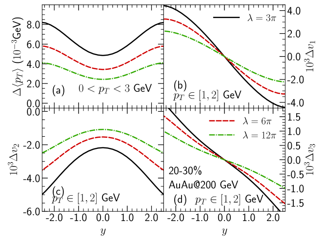
Figure 12: The dependence of the electromagnetically induced differences between the flow of protons and antiprotons on the choice of the drag coefficient $\mu m$ defined in Eq. (10). Elsewhere in this paper, we fix $\mu m$ by choosing the ’t-Hooft coupling in Eq. (10) to be $6\pi$. Here we explore the consequences of varying this parameter by factors of 2 and 1/2, thus varying $\mu m$ by factors of $\sqrt{2}$ and $1/\sqrt{2}$.

Throughout this paper, we have chosen fixed values for the two important material parameters that govern the magnitude of the electromagnetically induced contributions to flow observables, namely the drag coefficient $\mu m$ defined in Eq. (10) and the electrical conductivity $\sigma$. Here we explore the consequences of choosing different values for these two parameters.

In Fig. 12, we study the effect of varying the drag coefficient $\mu m$ on the the magnitude of the electromagnetically induced differences between the flow of protons and antiprotons. We change the value of the drag coefficient in Eq. (10) by choosing different values of the ’t Hooft coupling $\lambda$. (The consequences of varying $\mu m$ for the differences between the flow of $\pi^{+}$ and $\pi^{-}$ are similar, although the magnitude of the $\Delta v_{n}$’s is less for pions than for protons.) We see in Fig. 12 that all of the charge-dependent contributions to the flow that are induced by electromagnetic fields become larger when the drag coefficient $\mu m$ becomes smaller, as at weaker coupling. This is because the induced drift velocity $v_{\mathrm{drift}}^{\mathrm{\rm\,lrf}}$ in equation (9) is larger when the drag coefficient $\mu m$ is smaller. Since throughout the paper we have used a value of $\mu m$ that is motivated by analyses of drag forces in strongly coupled plasma, meaning that we may have overestimated $\mu m$, it is possible that in so doing we have underestimated the magnitude of the charge-odd electromagnetically induced contributions to flow observables.

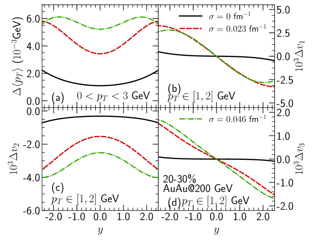
Figure 13: The dependence of the electromagnetically induced differences between the flow of protons and antiprotons on the choice the electrical conductivity $\sigma$ in the Maxwell equations (7) and (8).

In Fig. 13, we study the effect of varying the electrical conductivity $\sigma$ on the magnitude of the electromagnetically induced differences between the flow of protons and antiprotons. Note that, throughout, we are treating $\mu m$ and $\sigma$ as constants, neglecting their temperature dependence. This is appropriate for $\mu m$, since what matters in our analysis is the value of $\mu m$ at the freezeout temperature. However, $\sigma$ matters throughout our analysis since it governs how fast the magnetic fields sourced initially by the spectator nucleons decay away. The value of $\sigma$ that we have used throughout the rest of this paper is reasonable for quark-gluon plasma with a temperature $T\sim 250$ MeV, as we discussed in Section II. In a more complete analysis, $\sigma$ should depend on the plasma temperature and hence should vary in space and time. We leave a full-fledged magnetohydrodynamic study like this to the future. Here, in order to get a sense of the sensitivity of our results to the choice that we have made for $\sigma$ we explore the consequences for our results of doubling $\sigma$, and of setting $\sigma=0$.

The electromagnetically induced charge-odd contributions to the flow observables $\Delta\langle p_{T}\rangle$ and $\Delta v_{2}$ increase in magnitude if the value of $\sigma$ is increased. This is because the magnetic fields in the plasma decay more slowly when $\sigma$ is large Gursoy et al. (2014). And, a larger electromagnetic field in the local fluid rest frame at the freezeout surfaces induces a larger drift velocity which drives the opposite contribution to proton and antiproton flow observables. We see, however, that the increase in the charge-odd, rapidity-odd, odd $\Delta v_{n}$’s with increasing $\sigma$ is very small, suggesting a robustness in our calculation of their magnitudes. This would need to be confirmed via a full magnetohydrodynamical calculation in future. Since $\Delta\langle p_{T}\rangle$ and the even $\Delta v_{n}$’s are to a significant degree driven by Coulomb fields, it makes sense that they are closer to proportional to $\sigma$: increasing $\sigma$ means that a given Coulomb field pushes a larger current, and it is the current in the plasma that leads to the charge-odd contributions to flow observables. Although not physically relevant, it is also interesting to check the consequences of setting $\sigma=0$. What remains are small but nonzero contributions to $\Delta\langle p_{T}\rangle$ and the $\Delta v_{n}$. With $\sigma=0$ the electric fields do not have any effects during the Maxwell evolution; the small remnant fields at freezeout are responsible for these effects.

V Discussion and Outlook

We have described the effects of electric and magnetic fields on the flow of charged hadrons in non-central heavy ion collisions by using a realistic hydrodynamic evolution within the iEBE-VISHNU framework. The electromagnetic fields are generated mostly by the spectator ions. These fields induce a rapidity-odd contribution to $\Delta v_{1}$ and $\Delta v_{3}$ of charged particles, namely the difference between $v_{1}$ (and $v_{3}$) for positively and negatively charged particles. Three different effects contribute: the Coulomb field of the spectator ions, the Lorentz force due to the magnetic field sourced by the spectator ions, and the electromotive force induced by Faraday’s law as that magnetic field decreases. The $\Delta v_{1}$ and $\Delta v_{3}$ in sum arise from a competition between the Faraday and Coulomb effects, which point in the same direction, and the Lorentz force, which points in the opposite direction. These effects also induce a rapidity-even contribution to $\Delta\langle p_{T}\rangle$ and $\Delta v_{2}$, as does the Coulomb field sourced by the charge within the plasma itself, deposited therein by the participant ions. We have estimated the magnitude of all of these effects for pions and protons produced in heavy ion collisions with varying centrality at RHIC and LHC energies. Our results motivate the experimental measurement of these quantities with the goal of seeing observable consequences of the strong early time magnetic and electric fields expected in ultrarelativistic heavy ion collisions.

In our calculations, we have treated the electrodynamics of the charged matter in the plasma in a perturbative fashion, added on top of the background flow, rather than attempting a full-fledged magnetohydrodynamical calculation. The smallness of the effects that we find supports this approach. However, we caution that we have made various important assumptions that simplify our calculations: (i) we treat the two key properties of the medium that enter our calculation, the electrical conductivity $\sigma$ and the drag coefficient $\mu m$, as if they are both constants even though we know that both are temperature-dependent and hence in reality must vary in both space and time within the droplet of plasma produced in a heavy ion collision; (ii) we neglect event-by-event fluctuations in the shape of the collision zone; (iii) rather than full-fledged magnetohydrodynamics, we follow a perturbative calculation where we neglect backreaction of various types, including the rearrangement of the net charge in response to the electromagnetic fields; (iv) we assume that the force-balance equation (9) holds at any time and at any point on the plasma, meaning that we assume that the plasma equilibrates immediately by balancing the electromagnetic forces against drag. As we shall discuss in turn, relaxing these assumptions could have interesting consequences, and is worthy of future investigation. But, relaxing any of these assumptions would result in a substantially more challenging calculation.

Relaxing (i) necessitates solving the Maxwell equations on a medium with time- and space-dependent parameters, which would result in a more complicated profile for the electromagnetic fields. We expect that this would modify our results in a quantitative manner without altering main qualitative findings. We have tried to choose a value for $\sigma$ corresponding roughly to a time average over the lifetime of the plasma and a value of $\mu m$ corresponding roughly to its value at freezeout, which is where it is relevant to our analysis. The values of each could be revisited, of course, but our investigation in Section IV.2 indicates that this would not affect any qualitative results.

Relaxing (ii), which is to say adding event-by-event fluctuations in the initial conditions for the hydrodynamic evolution of the matter produced in the collision zone, as well as for the distribution of spectator charges, would have quite significant effects on the values of the charge-averaged $\langle p_{T}\rangle$ and $v_{n}$’s, for example introducing nonzero $v_{1}$ and $v_{3}$. Solving the Maxwell equations on such a medium would of course be much more complicated. Furthermore we expect that consequences would appear in all four of the electromagnetic effects that we have analysed (the Faraday $\vec{E}_{F}$, the Lorentz $\vec{E}_{L}$, the Coulomb field of the spectators $\vec{E}_{C}$ and the Coulomb field of the plasma $\vec{E}_{P}$) resulting in each contributing at some level to each of the four observables that we have analysed ($\Delta\langle p_{T}\rangle$, $\Delta v_{1}$, $\Delta v_{2}$ and $\Delta v_{3}$). However, we expect that the electromagnetically induced contributions that we have found using a smooth hydrodynamic background without fluctuations, and whose magnitudes we have estimated, will remain the largest contributions.

Relaxing assumption (iii) may bring new effects and, as we shall explain, could potentially flip the sign of the odd flow coefficients $\Delta v_{1}$ and $\Delta v_{3}$. One particular physical effect that we neglect is the shorting, or partial shorting, of the Coulomb electric fields in the plasma, both the $\vec{E}_{C}$ sourced by the spectators and the $\vec{E}_{P}$ sourced by the plasma itself. These Coulomb fields will push charges in the plasma to rearrange in a way that reduces the electric field within the conducting plasma. We have neglected this, and all, back reaction in our calculation. However, although it would require a fully dynamical calculation of the currents and electric and magnetic fields to estimate its extent, some degree of shorting must occur. There may, in fact, be experimental evidence of this effect: $\Delta v_{2}$ for pions has been measured in RHIC collisions with 30-40% centrality and collision energy $\sqrt{s}=200$ AGeV by the STAR collaboration Adamczyk et al. (2015), and although it turns out to be negative as our calculations predict it is substantially smaller in magnitude than what we find. Because there are other effects (unrelated to Coulomb fields) that can contribute to $\Delta v_{2}$ and that are known to contribute significantly to $\Delta v_{2}$ in lower energy collisions Xu et al. (2012); Steinheimer et al. (2012); Ko et al. (2014); Adamczyk et al. (2013); Xu et al. (2014); Adamczyk et al. (2016); Xu and Ko (2016), it would take substantially more analysis than we have done to use the experimentally measured results for $\Delta v_{2}$ to constrain the magnitude of $\vec{E}_{C}$ and $\vec{E}_{P}$ quantitatively. However, it does seem likely that, due to back reaction, they have been at least partially shorted, making them weaker in reality than in our calculation.

The likely reduction in the magnitude of $\vec{E}_{C}$, in turn, has implications for the odd $\Delta v_{n}$’s. Recall that they arise from the sum of three effects, in which there is a near cancellation between $\vec{E}_{F}+\vec{E}_{C}$ and $\vec{E}_{L}$, which point in opposite directions. The sign of the rapidity-odd $\Delta v_{1}$ and $\Delta v_{3}$ that we have found in our calculation corresponds to $|\vec{E}_{F}+\vec{E}_{C}|$ being slightly greater than $|\vec{E}_{L}|$. If $|\vec{E}_{C}|$ is in reality smaller than in our calculation, this could easily flip the sign of $\Delta v_{1}$ and $\Delta v_{3}$. In this context, it is quite interesting that a preliminary analysis of ALICE data Margutti (2017) indicates a measured value of $\Delta v_{1}$ for charged particles in LHC heavy ion collisions with 5%-40% centrality and collision energy $\sqrt{s}=5.02$ ATeV that is indeed rapidity-odd and is comparable in magnitude to the pion $\Delta v_{1}$ for collisions with this energy that we have found in Fig.10, but is opposite in sign.

Finally, let us consider relaxing our assumption (iv). This corresponds to considering a more general version of (9) with a non-vanishing acceleration on the right-hand side. The drift velocity that would be obtained in such a calculation would decay to the one that we have found by solving the force-balance equation (9) exponentially, with an exponent controlled by the drag coefficient $\mu$. Thus, for very large $\mu$ we do not expect any significant deviation from our results. However, at a conceptual level relaxing assumption (iv) would change our calculation significantly, since it is only by making assumption (iv) that we are able to do a calculation in which $\mu$ enters only through the value of $\mu m$ at freezeout. If we relax assumption (iv), the actual drift velocity would always be lagging behind the value obtained by solving (9), and determining the drift velocity at freezeout would, in principle, retain a memory of the history of the time evolution of $\mu$. If we use the estimate (10) for $\mu$ and focus only on light quarks, and hence pions and protons, as we have done we do not expect that relaxing assumption (iv) would have a qualitative effect on our results. However, $\mu$ may in reality not be as large as that in (10) at freezeout. And, furthermore, it is also very interesting to extend our considerations to consider heavy charm quarks, as in Ref. Das et al. (2017). The charm quarks receive a substantial initial kick from the strong early time magnetic Das et al. (2017) and electric fields, and because they are heavy $\mu$ may not be large enough to slow them down and bring them into alignment with the small drift velocity that (9) predicts for heavy quarks. Hence, consideration of heavy quarks requires relaxing our assumption (iv) in a way that alters our conclusions significantly, and indeed the authors of Ref. Das et al. (2017) find a substantially larger $\Delta v_{1}$ for mesons containing charm quarks than the $\Delta v_{1}$ that we find for pions and protons. These considerations motivate the (challenging) experimental measurement of $\Delta v_{1}$ for $D$ mesons.