Limiting Behaviors of High Dimensional Stochastic Spin Ensembles
Abstract
Lattice spin models in statistical physics are used to understand magnetism. Their Hamiltonians are a discrete form of a version of a Dirichlet energy, signifying a relationship to the Harmonic map heat flow equation. The Gibbs distribution, defined with this Hamiltonian, is used in the Metropolis-Hastings (M-H) algorithm to generate dynamics tending towards an equilibrium state. In the limiting situation when the inverse temperature is large, we establish the relationship between the discrete M-H dynamics and the continuous Harmonic map heat flow associated with the Hamiltonian. We show the convergence of the M-H dynamics to the Harmonic map heat flow equation in two steps: First, with fixed lattice size and proper choice of proposal size in one M-H step, the M-H dynamics acts as gradient descent and will be shown to converge to a system of Langevin stochastic differential equations (SDE). Second, with proper scaling of the inverse temperature in the Gibbs distribution and taking the lattice size to infinity, it will be shown that this SDE system converges to the deterministic Harmonic map heat flow equation. Our results are not unexpected, but show remarkable connections between the M-H steps and the SDE Stratonovich formulation, as well as reveal trajectory-wise out of equilibrium dynamics to be related to a canonical PDE system with geometric constraints.
1 Introduction
The Metropolis-Hastings (M-H) algorithm [19] is widely used in particle statistics for model estimations [36, 5, 29, 4, 34]. It constructs a discrete-time Markov chain to sample a desired probability distribution by accepting or rejecting proposed states. For applications in statistical physics, it is often the Gibbs or canonical distribution that is to be sampled. In this case, the algorithm accepts all the proposed new states with lower energy and often rejects the proposals with higher energy. Similar sampling can be achieved simulating a Langevin Stochastic differential equation (SDE) that performs gradient descent with noise; it too has the Gibbs distribution as its steady-state distribution. This suggests that the Langevin SDE might be the optimal M-H algorithm in which all proposals are accepted.
For certain forms of probability distributions, the diffusion limit and therefore optimal scaling, of the random walk M-H algorithm has been obtained [39, 6, 35]. Specifically, for product measures in [39] and the Gibbs distribution of a lattice model in [6], the weak convergence to Langevin diffusions has been shown by comparing generator functions. For non-product form measures the weak convergence to a stochastic partial differential equation was shown in [35]. These works consider the weak convergence only in equilibrium. Subsequent works [22, 23] consider scaling limits of out of equilibrium systems approaching equilibrium, but for product measures. In this work, we fill a missing gap in the above mentioned works of trajectory-wise convergence, without assuming the system is in equilibrium, for non-product measures.
To address the question of trajectory-wise convergence, we study the XY and the classical Heisenberg lattice spin models [40] that play an important role in statistical physics to understand phase transitions and other phenomena including superconductivity [28, 12]. It is important to understand the limiting behavior of these models, including optimal scalings for simulations, and their critical properties. For example, asymptotic results on the total spin of the mean-field XY and classical Heisenberg models have been studied by large deviation theory and Stein’s method in [25, 26]. Numerically, Monte Carlo methods are used to verify analytical results about the XY model in [34, 4] and the classical Heisenberg model in [38, 7].
The XY and classical Heisenberg models are defined on a periodic -dimensional lattice with the distance between adjacent vertices. Each spin sits at a lattice point and is described by a unit vector , for where for the XY model and for the classical Heisenberg model. We will focus primarily on the case of , but continue the discussion for general as the trajectory-wise convergence should follow similarly. The calculation from M-H to SDE should follow for higher dimension ; SDE to PDE depends on the smooth solution of harmonic map heat flow equation, which we only have guaranteed for all time in the case using for instance the work [15]. Here we assume that we are looking on a time scale for which the PDE has a smooth solution and focus on comparing to the microscopic dynamics. It is an interesting topic for future work to study the nature of singularity formation in the microscopic and mesoscopic models.
The Hamiltonian of the system,
| (1) |
gives energy to misaligned neighboring spins where represents nearest neighbors and is a scaling factor. Denote as the total spin configuration of , the M-H algorithm accepts/rejects based on the Gibbs distribution defined as
| (2) |
where is the inverse temperature and is the normalizing factor (aka partition function).
We will show that the M-H algorithm applied to the above lattice system, in the limit of small perturbations in the proposal, produces equivalent trajectories to the overdamped Langevin equation,
| (3) |
(interpreted in the Stratonovich form) where the are -dimensional independent Brownian motions, is the discrete Laplacian and for is the projection of onto the tangent plane of . We find that the exact form of the projection does not matter, for example one could take either or when . The Stratonovich understanding of (3) is essential to keep the as unit vectors, and for more on this equation see [2]. Our proof in section 3 naturally leads to the Itô form of equation (3), which includes an additional Itô correction term of . This (overdamped) Langevin system (3) performs gradient descent on the energy defined by (1) with the added constraint that is confined to , . In the case of for the classical Heisenberg model, it is an SDE representation of the overdamped Landau-Lifshitz-Gilbert equation that has the Gibbs distribution as its invariant measure [2, 27].
Taking the number of lattice points, , to infinity or equivalently the lattice spacing to zero, the limit of the deterministic part of (3) is the partial differential equation (PDE) called the harmonic map heat flow equation
| (4) |
In the case, (4) is in the form of the overdamped Landau-Lifshitz equation [14]
| (5) |
In [15] this Landau-Lifshitz equation was shown to be equivalent to the Harmonic map heat flow from . With the scaling , the Hamiltonian in (1) is the discrete form of the Dirichlet energy, , for this harmonic map heat flow. This suggests that by decreasing the temperature, the out of equilibrium dynamics of the M-H algorithm converge to the deterministic flow of (5) with large for the classical Heisenberg model. We will show this equivalence by showing the convergence of the system of SDEs (3) to the PDE (4) in the limit of large with an appropriate scaling of the temperature to zero with . We point out that in order to obtain the finite temperature Stochastic PDE limit of the M-H dynamics in arbitrary dimension required a regularization of the noise. We intend to pursue deriving a stochastic PDE limit of the M-H algorithm using colored noise in the proposal for future work.
While this current work does not focus on the dynamics of equation (4), we point out that much work has been done on harmonic maps, the evolution of deterministic and stochastic harmonic map heat flows, as well as on describing the potential for singularity formation. We cite for instance the now classical works of Eells and Sampson on Harmonic Maps [11] and of Struwe [41], and the subsequent works of Chen-Struwe and Chen [9, 8]. Rigidity and singularity formation was further understood in the works of Topping on the evolution of harmonic map heat flows and singularity formation [44, 42, 43], and the works of Lin-Wang [32, 30, 31]. We also note the book [33] for a useful background on the subject. The literature on the Harmonic Map Heat Flow is quite extensive and we do not suggest that the list here is complete.
Though we do not establish the connection between the M-H dynamics and the Stochastic Harmonic Map Heat Flow in this work, these equations have also been studied recently. We cite again the book [2] by Banas-Brzezniak-Neklyudov-Prohl that has many useful results in it about Stochastic ODE approximations and analysis of many aspects of the full Landau-Lifshitz-Gilbert stochastic PDE version of the full Landau-Lifshitz equation, which is a PDE similar to the harmonic map heat flow but including both dissipative and dispersive components of the flow. We also cite more recent works on dynamics of stochastic Harmonic Map Heat Flow equations, including the works of Guo-Philipowski-Thalmaier [16], Hocquet [20, 21], Chugreeva-Melcher [10]. For works on numerical discretization in a semi-discrete fashion of the stochastic Landau-Lifshitz equation, see the work of Alouges-De Bouard-Hocquet [1].
One method to obtain the deterministic limit of a stochastic system is to consider the hydrodynamic limit with relative entropy bounds [17, 46, 13]. Due to the geometric constraint in the XY and classical Heisenberg models, it is difficult to calculate the averages with respect to the Gibbs states as in [17, 46, 13] if the spin is expressed in Cartesian coordinates. One might try to use polar coordinates to do window averaging but the potential is not convex as in [13]. Since the hydrodynamic limit for the XY and the classical Heisenberg models are not fully understood, we choose an alternative approach of taking inverse temperature to infinity along with particle number .
One challenge in showing convergence of the spin models to diffusions is that the distribution (2) is unaware of the confining geometry that the spins must remain in . Rather, it is included in the proposal step of the M-H algorithm. Therefore, simply considering the equilibrium distribution is not enough to show equivalence, the proposal step must be taken into account for a trajectory-wise comparison between processes. While always accepting the proposal step leads to each spin behaving independently like Brownian motion on the surface of , sampling a product measure, to consider the true M-H algorithm sampling (2) we must therefore take into account the interdependence of the spins.
Working directly with the proposal step, which includes a normalizing step, also includes challenges. To linearize the nonlinear dynamics, we take the Taylor expansion of the M-H step and approximate it as a linear step. The challenge here is that the coefficients of this expansion are random variables that can be arbitrarily large, therefore bounding the error is not trivial. Also, the truncation of the proposal leads to a spin vector that does not stay on the sphere. However, this displacement from the sphere is small, converging to zero as the size of the proposal tends towards zero.
Note that in the weak convergence result of M-H dynamics to diffusion processes [39, 6, 35], the assumption of equilibrium is essential to bound the error terms. The result in this paper only assumes that the M-H dynamics (and thus the SDE system) start from a deterministic initial condition satisfying a certain regularity condition. While the initial condition is assumed smooth, both the M-H and SDE dynamics immediately produce fluctuations, and the resulting trajectories are only close to the smooth deterministic PDE solution and not smooth themselves for all time. Therefore, standard energy bounding techniques cannot be used. To bound the error terms, we utilize scalings that are worse than those in the previously mentioned papers and are likely not optimal. We use numerical simulations to explore how tight these bounds appear to be.
The remainder of the paper is as follows. In Section 2 we present the main results in two parts. First, we state the convergence of M-H dynamics to the SDE system (3) as the proposal size of M-H step goes to zero, then we state the convergence of the SDE system (3) to the deterministic PDE (4) as the lattice size goes to infinity and temperature to zero. The key steps of the proofs are given in Sections 3 and 4 for the more complicated classical Heisenberg model from with details appearing in the Appendix. The proof for the XY model follows similarly. For the M-H to SDE (3) proof in Section 3, we apply a similar approach as in [35], by first Taylor expanding the M-H step, keeping only the first three terms, then computing the required conditional expectations with respect to the Gaussian random variables to obtain the drift and diffusion terms of an Euler step for the diffusion process. Then, the difference between the M-H and SDE dynamics in norm is bounded by a Grönwall inequality. For the SDE (3) to PDE (4) proof in Section 4, we compare the SDE system with the finite difference approximation of the harmonic map heat flow equation (4). The difference between the SDE and ODE system is governed by another diffusion process. We will rescale this process and show the rescaled error is bounded for a long time using stopping time. These convergence results are compared to the convergence measured from the results of numerical simulations of the system in Section 5. Conclusions are presented in Section 6.
Remark 1.1.
We only show the case . The calculation could be generalized for other cases of quite similarly.
2 Main Results
In this section we will explain how we apply the M-H algorithm to the XY and classical Heisenberg models, and state our main results. Our first result is that the M-H dynamics is close to a stochastic Euler scheme for the SDE (3) in Itô form. The bound on the error between the M-H dynamics and the SDE (3) is accomplished using arguments similar to the convergence of the stochastic Euler method. Our second result bounds the error between the SDE system and the finite difference approximation of the harmonic map heat flow equation (4).
Throughout the paper, we adopt the following notation. We use the symbol when describing random variables. For example, denotes that random variable is distributed with a normal distribution with mean 0 and variance 1. For approximating deterministic functions, we use the notation as to indicate that is of lower order than , specifically that . When we approximate random variables, we use the notation as the difference between the variable and its approximation could be extremely large in a single realization, and therefore the notion of asymptotic approximation does not hold. Therefore, when using the notation that random variable we mean that the random variable has a deterministic prefactor that this .
2.1 Metropolis-Hastings step.
Here, we explicitly state the M-H dynamics for the XY and classical Heisenberg models with Hamiltonian given by (1) for the case .
Consider a set of spins evolving in time, for particles and time step , with time step size . To create the proposal, take the normal random vector
for the XY model and three-dimensional normal random vector
for the classical Heisenberg model. Then project this noise vector onto the tangent plane of , forming the random vector
| (6) |
Since we are proving a trajectory-wise convergence result, we must imbed the M-H algorithm and the SDE dynamics in the same probability space. To this end, we define
where are the independent Brownian motions in (3).
In the M-H algorithm, the intuitive idea for a proposal, , on a manifold at time-step is the exponential map
| (7) |
where is the geodesic satisfying the nonlinear ODE with the affine connection on the manifold and is the proposal size. In practice, using the proposal
is computationally simpler and, as we will show, leads to the same convergence result.
The values and are used to denote the total spin configuration at time step and the total proposal spin configuration . The proposal is accepted with probability
| (8) |
and rejected otherwise, where
| (9) | |||
is the difference between the Hamiltonian (1) of the proposal and of the current spin configuration . Then
Repeating the proposal and accept/reject steps, we create a discrete Markov process at time steps and we will show the convergence of the Markov chain to the solution to the Langevin SDE system (3).
2.2 Convergence of Metropolis dynamics to SDE system.
First we will show the convergence from the M-H dynamics to the Langevin SDE dynamics with a fixed number of particles as the proposal size . Intuitively, using the Taylor series truncation of the proposal, the approximation of one M-H step leads to an expression that looks like one Euler step for simulating the SDE (3) in Itô form.
Let denote the filtration generated by the set of Brownian motions , i=1…N, in (3) and Bernoulli random variables , . We denote the conditional expectation by .
The drift over one step of the Metropolis-Hastings algorithm for the -th particle for small is approximated by
| (10) |
where is the projection onto the tangent plane of .
Denoting the noise contribution over one step as
| (11) |
it is approximated by
| (12) |
Thus, one step of the Metropolis-Hastings algorithm is approximately given by
| (13) |
Defining where is the time step size, the above equation changes to
| (14) |
Since and when , the above is the Euler step for the Langevin SDE (3) in Itô interpretation
| (15) |
This intuitive idea leads to the first result:
Theorem 2.1.
Define the piecewise constant interpolation of M-H dynamics as ,
| (16) |
and as the solution for the Langevin SDE system (15) with initial condition , . If the noise used in the proposal for each M-H step is related to the Wiener processes driving the SDE as , then we have the following strong convergence result:
| (17) |
for any , where are functions of and independent of the choice of and .
Remark 2.2.
Remark 2.3.
Theorem 2.1 is a trajectory-wise convergence result.
2.3 Convergence of SDE system to the Harmonic map heat flow equation.
Notice in the SDE (15), if is chosen to be , formally the noise part disappears with . This gives the idea of the second result:
Theorem 2.2.
For the harmonic map heat flow equation (4) with periodic boundary conditions and initial condition satisfying
| (18) |
for some as in [15], the solution exists and is smooth. Denote the finite difference approximation of (4) as
| (19) |
By [45, Theorem 1], the difference between the solution to this finite difference approximation and the PDE (4), , goes to zero on any fixed time interval where the solution remains well defined, as the space discretization goes to zero.
Since is equivalent to with the defined scaling of , and , the quantity is small when is large, going to zero as . Since the solution to the PDE is smooth, satisfying the conditions in (18), the finite difference approximation is close to the PDE solution as shown in [45], going to zero as . Therefore, at a fixed time , the difference between the SDE system (15) and the PDE (4) goes to zero as .
Remark 2.4.
The choice of depends on through the following relation
which is equivalent to
since . For a uniform bound in an interval , we need which requires . For a bound at a fixed time , we only need and thus require . We do not believe this bound is sharp for the convergence result, which will be addressed in Section 5 when we perform numerical simulations of these models. We find that is enough to see convergence in our numerical simulations. Using an approximation of being near equilibrium, it is possible to use sharper bounds on summation in from the regularity properties of the invariant measure to improve , but we do not pursue such techniques here.
3 Metropolis-Hastings dynamics to SDE system
In this section the convergence of the M-H algorithm to the SDE (15) for the classical Heisenberg model will be shown by calculating the drift and diffusion of one M-H step, which is approximately a stochastic Euler step for (15). Then the error estimation of stochastic Euler’s method is used to give a bound on the difference between M-H and SDE dynamics with proposal size . Here the basic steps are outlined, the detail of error estimation is given in Appendix A.
Remark 3.1.
The proof for the XY model will be similar, one only needs to change the random vector on the tangent plane to a two-dimensional vector.
3.1 Set-up.
In the calculation to follow, we have the following assumptions and notations. The number of the particles on unit length is fixed and the limiting case is considered. We have as functions of so they are also regarded as constant. On the unit sphere, the proposal is given by the exponential map (7) and could be approximated by normalizing
By Taylor expanding , the proposal can be approximated by order and expansion
| (21) | ||||
The proof of the following Lemma is shown in Appendix A.
Lemma 3.1.
Denote
Then and .
3.2 Drift.
Proposition 3.1.
Let be the Markov chain given by the Metropolis-Hastings algorithm, and the spin for -th particle at time step . Then
| (23) |
where the error term
| (24) |
satisfies .
In the calculation we keep the order term. The remainder is order and will be shown to be bounded in the error estimation for M-H and SDE dynamics. The basic steps are given in the following calcuation, for details of the error estimation see Appendix A.
Since with probability and stay otherwise,
| (25) | ||||
We drop the third term in the last line of (25) as it is an term:
since for finite . For the second term in the last line of (25), since we have that
This corresponds to the Itô correction term for (3).
The first term in the last line of (25) is the most difficult one to approximate. Using the notation in (22)
since , to write it as
For any orthonormal basis in , the normal random vector can be expressed as
and are independent standard normal random variables. Denote ,. Choose two orthonormal vectors on the tangent plane of and ,
where are independent. Then,
| (26) | ||||
The two terms on the right are similar in form so we only show the calculation for the first one and the second one follows similarly.
Remark 3.2.
For the XY model, the projection of the normal random vector onto the tangent plane of is represented by the form , where . The other parts of the calculation basically stays the same.
Using tower property of conditional expectation for the first term on the RHS of (26), we have
Lemma 3.2.
For ,
| (27) |
for any real constants , and is the CDF for the standard normal random variable.
The proof of this Lemma is the direct result of the integration for the expectation. And the Lemma gives
| (28) | ||||
Before taking the expectation over , we further simplify this expression by noting that resulting in
| (29) | ||||
For a mean zero Gaussian random variable , we know
as is an odd function and the probability density function is even.
Notice that is a sum of independent mean zero Gaussian random variables, so is a Gaussian random variable with mean , therefore
The second term on the RHS of (26) follows similarly,
Combining the above
where and denotes the discrete Laplacian.
3.3 Diffusion.
Recall in (11),
with accept rate in (8). Since is an order term and with small , we are going to show
Proposition 3.2.
The diffusion term
| (30) |
where
| (31) |
is a random variable with mean , variance , and covariance for .
Proof.
For the mean
then .
For the variance,
| (32) | ||||
For the second term in the last line of (32), since , we observe that
for some constant . We have used that and are both order term.
Combining the above, the variance in (32) is bounded by .
For the covariance of at different time steps , and denotes the coordinates of the vector,
∎
3.4 Proof of Theorem 2.1
For the error estimation, we apply similar techniques as in the proof of stochastic Euler’s method.
Take as in Theorem 2.1. For simplicity we denote
| (33) |
as the drift and diffusion coefficients in (15), respectively, where is the collection of all the . When are fixed and , the coefficient and are Lipschitz continuous in each coordinates of . From Theorem 5.2.1 in [37], the SDE system has a unique solution.
Now we have the following estimate on the error.
Proposition 3.3.
Define the error between M-H interpolation and SDE (15) solution as
| (34) |
For any fixed , is bounded by
| (35) |
Proof.
For the proof we are going to show satisfies the Grönwall inequality ( denotes some constant bound):
| (36) |
so .
Since and both start from the same initial condition, from the definition of and in (24), in (11), in (31) we have that
| (37) |
where and . Applying Hölder’s inequality and produces
| (38) |
Using Hölder inequality for the first term in (3.4) with the coordinate
since is Lipschitz,
combine terms,
Applying Itô isometry to the second term of (3.4) for the coordinate
Since
then
and coordinates of the second term in (3.4) are similar. Summing up coordinates, the second term in (3.4) is bounded by
Apply Itô isometry again for the fourth term in (3.4),
Remark 3.4.
In the Grönwall inequality, the term decides the order of convergence. It comes from , which we show is an term in A.3.
With Proposition 3.3, we can get a uniform bound by using Doob’s martingale inequality in [37] for a nonnegative submartingale and constant :
| (39) |
Proposition 3.4.
Define the error between M-H and SDE dynamics for -th spin as
| (40) |
for any . There exists some constant as a function of and independent of ,
| (41) |
for any .
Proof.
Similar to (3.4) in Proposition 3.3, we have that
| (42) |
and each term on the RHS will be bounded by for some constant . Applying Hölder’s inequality for the first term in (3.4):
The last inequality above is from in Proposition 3.3.
For the second term in (3.4), the length of the interval of integration is smaller than and as , so
| (43) |
The integral in the third term of (3.4) is a martingale. For , denote
This is a Martingale and is a nonnegative submartingale, hence by Doob’s inequality (39)
For a nonnegative submartingale
Applying Itô isometry for the last term similar to the proof of Proposition 3.3 and summing for all coordinates :
From Cauchy inequality, the fourth term in (3.4)
from Proposition 3.1 so the last expectation is bounded by .
In the fifth term of (3.4), is a discrete martingale. Again using martingale inequality for each coordinate and then summing up,
| (44) |
from 3.2 , it is bounded by
| (45) |
Combining the above, (41) is obtained. ∎
4 From SDE system to deterministic PDE
In this section, we explain the convergence from the SDE system (15) to the deterministic harmonic map heat flow equation without the dispersion term (5) with proper choice of and number of particles .
Remark 4.1.
From [15], for sufficiently regular initial data, there exists a global smooth solution to the Landau-Lifshitz equation
| (46) |
with periodic boundary conditions, and some constants. From [45], it is known that the finite difference approximation converges to the Landau-Lifshitz equation (46). The harmonic map heat flow equation (4) only has the dissipation term of the Landau-Lifshitz equation (46) and the results from [45] should still hold. We will assume a global smooth solution exists for the harmonic map heat flow equation (4) in all contexts below. The finite difference approximation (19) will converge to the harmonic map heat flow equation (4) as and we only need to compare the SDE system (15) and the ODE system (19).
In the following the error between (15) and (19) is calculated. Since and , we denote
| (47) |
as a small parameter going to zero with . The SDE is then written as
| (48) |
Lemma 4.1.
Proof.
Taking the projection given by
together with , we have that
where . The SDE system (48) can then be written as
and the ODE system (19) can similarly be written as
By definition satisfies the following equation
Since with ,
| (51) |
Applying Itô’s formula to , we have that
where represents the Itô correction term of order as shown in the following computation.
To calculate the Itô correction we consider the SDE systems for both in (51) and in (15). The Itô correction for combines three parts corresponding to and . Since we take as bounded by . The first term, , is a constant and . The second term, , is order but is order so the Itô correction for the second term is also . For the third term but so the Itô correction for the third term is also .
Returning to , from the periodic boundary conditions, we know that
hence summing up we have that
| (52) |
For the second term of (4), from the Cauchy-Schwarz inequality, we observe that
Since the solution for the harmonic map heat flow equation is smooth, in the third term of (4), can be bounded by some constant . For the fourth term in (4) since . Hence from (4),
Using the assumption that , (or equivalently ,) we bound the term by . Hence,
| (53) |
as the p-norm is decreasing. Finally, since , we arrive at (50).
∎
Remark 4.2.
If we choose the parameters such that the small Itô correction term, , from the martingale is of lower order in and , (or equivalently ,) we could show a similar result for instead of . We could then bound .
Intuitively the inequality from Lemma 4.1 is of Grönwall type and the martingale part,
has a small coefficient . This implies that with large probability
and is bounded for a long time interval. We use this idea to show the following proposition.
Proposition 4.1.
| (54) |
for some constant and satisfying .
To prove Proposition 4.1, we will use the exponential martingale inequality for continuous martingale as in [18, p. 25] or [3] :
| (55) |
where is the quadratic variation for .
For the martingale in (50), we calculate its quadratic variation in the following lemma.
Lemma 4.2.
The quadratic variation for the martingale
is
| (56) |
Proof.
The quadratic variation for is captured by a direct summation of the square of the coefficients of the white noise, namely
∎
Now taking and in the inequality (55), we have that
| (57) |
Thus, with probability , the following inequality holds
Combining this with (50), we observe that
| (58) |
where we have used the definition of and that .
Since (4) is a Grönwall type inequality, we build a special upper solution . Then
where when . We observe that
so . As , we have that
| (59) |
and is an upper bound for .
4.1 Proof of Theorem 2.2
When is small enough we have that and is an upper bound for . We observe that with ,
| (60) |
and the inequality in Proposition 4.1 follows.
In fact, as , the bound by some constant is sufficient. Appealing to a stopping time argument similar to the strong uniqueness proof of the SDE with locally Lipschitz continuous coefficients (see e.g. [24, Chapter 5.2,Theorem 2.5]), we have the following result.
Proposition 4.2.
Given , there exists a constant independent of such that if , then
Proof.
Define a deterministic time and a stopping time . Since , we have both and . If is infinite then we are done, so assume is bounded.
From Lemma 4.1,
| (61) |
As , we have that
| (62) |
and as , so
| (63) |
Taking the expectation on both sides, we arrive at the fact that
| (64) |
The expectation can be deduced from the optional stopping theorem for continuous time or take . Notice , so
and by a Grönwall’s inequality,
| (65) |
Choosing , the result follows.
∎
By similar arguments, a uniform bound on can be obtained with a weaker condition on .
Proposition 4.3.
Given , there exist constants independent of such that if , for , then
Proof.
Define and . Since we still have .
Again from Lemma 4.1, we observe that
| (66) |
Taking the supremum on both sides, we arrive at the fact that
| (67) | ||||
The above, together with and , gives
| (68) |
Taking expectations on both sides, we arrive at the fact that
| (69) |
For the first integral on the right hand side, we note that . Doob’s Martingale inequality (39) is used to give a bound of for the last expecation in (69).
Denote
Since , the above is a martingale. Using Doob’s martingale inequality (39) we have that
The second equality is from Itô isometry and the third inequality is because so and .
Now a Grönwall’s inequality gives
| (70) |
and . As in the proof of the previous Proposition, choosing and , and assuming , the result thus follows similarly.
∎
5 Numerical results
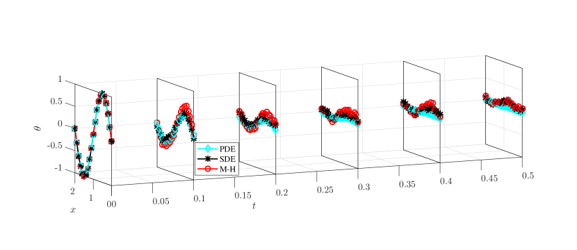
In this section, we present results from numerical simulations of the systems, showing both the temporal dynamics and the order of convergence. The numerical convergence tests indicate that the error decays at least as well as predicted in Theorems 2.1 and 2.2. We check both the cases of the XY model and the classical Heisenberg model. The dynamics of the M-H algorithm are simulated as explained in Sec. 2.1. To simulate the SDE (15), written in the Itô sense, we use the stochastic Euler’s method combined with a normalizing step to project the spin back onto the sphere after each time step for both the XY model and the classical Heisenberg model. The PDE (5) is numerically integrated by discretizing in space and using the Euler’s method presented in [45] which includes a normalization step.
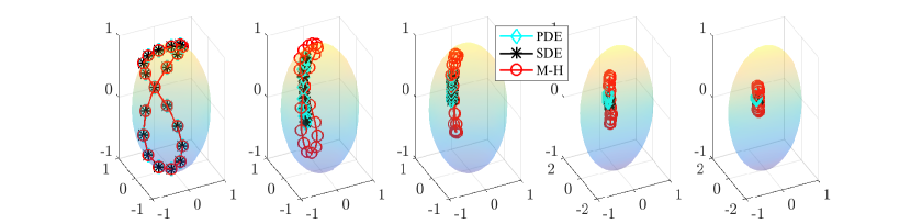
The out-of-equilibrium to equilibrium dynamics of the M-H algorithm, SDE, and discretized PDE are shown in Figure 1. Figure 1(a) shows the case of the XY model in terms of the polar coordinate of each spin. Figure 1(b) shows the case of the classical Heisenberg model with each spin plotted on the same unit sphere; nearest neighbors are connected by a solid line. In both cases, the M-H dynamics tend to lag behind the SDE and PDE which more closely follow each other. This suggests the error between the M-H algorithm and the PDE is dominated by the error between the M-H algorithm and the SDE. Thus the order of convergence between M-H algorithm and harmonic map heat flow equation should almost follow the order of convergence in Theorem 2.1.
Figures 2 and 3 show the order of convergence for the error between the M-H algorithm and the Langevin equation with respect to the time step size , for which the equivalent M-H proposal size is . The error is calculated at a fixed time as
| (71) |
where the expectation is taken over multiple realizations. All four frames support that the convergence is at least as good as , which is equivalent to the convergence given in Theorem 2.1, since the 2-norm is used in the numerical experiments (thus the error is expected to be of order ). The faster convergence of order in panels (b) and (c) of Fig. 2 we suspect is due to the fact that these out-of-equilibrium dynamics are dominated by the deterministic part of the SDE, and this part has different error scaling from the noisy dynamics. In equilibrium, the deterministic term, , is small since it is zero at the minimum of the Hamiltonian (maximum of the Gibbs distribution), and the noisy part of the dynamics dominate.
Proposition 3.1 states the error on the deterministic drift of one Metropolis step, , is of size . Dividing by a time-step that is proportional to so that the left-hand side approximates a derivative for the SDE, the resulting error is or equivalently as seen in the numerical simulations. Similarly, from Proposition 3.2 the error on the stochastic diffusion of one Metropolis step, , is of size implying error of order , after dividing by the size of the first order term, . To further test if the difference in convergence order is from the deterministic terms dominating, we increase the size of the noise, , in Eq. (15) by decreasing to make the noisy dynamics dominate. The out-of-equilibrium error with small shown in Fig. 3 has convergence, confirming the original statement of Theorem 2.1. We therefore conclude that the error bound of is tight, and this error comes from the noisy part of the dynamics.
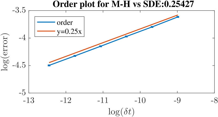
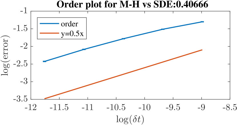
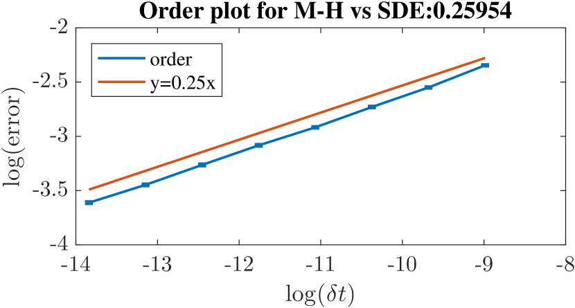
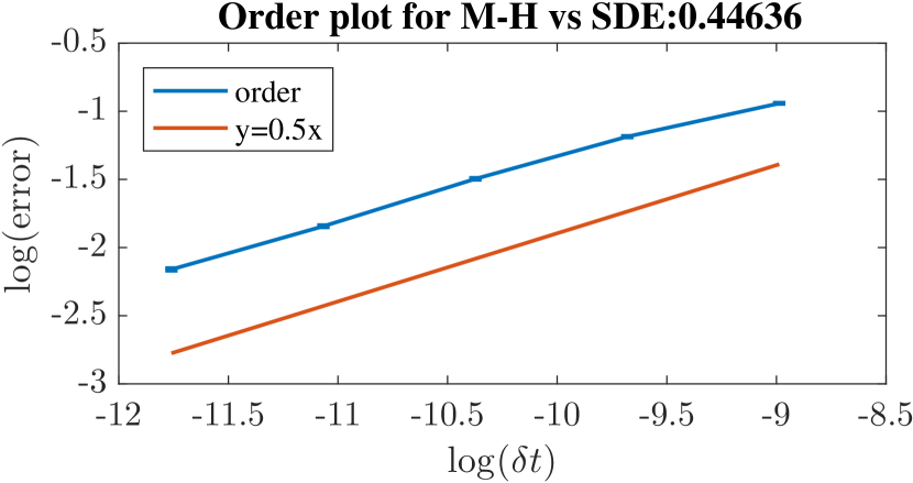
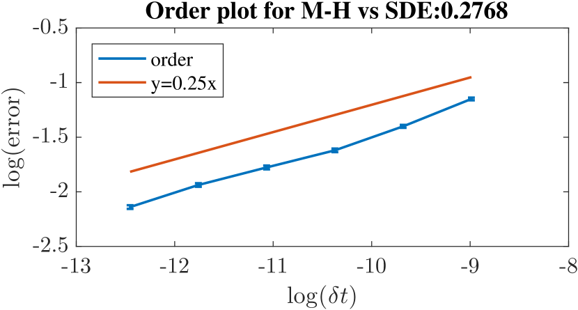
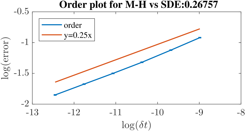
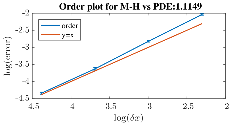
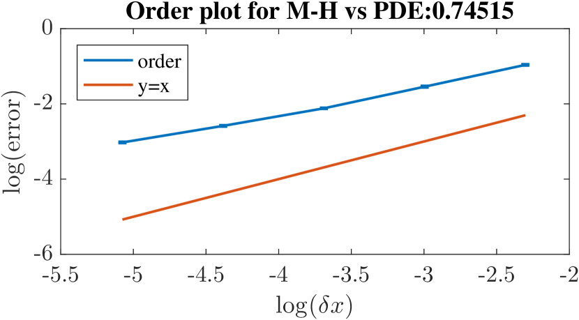
Figure 4 shows the convergence test for the error between the M-H and the PDE dynamics with respect to . The discrete version of the PDE is simulated with the time-step scaling of and , which are also used with in the M-H algorithm. These scalings give the order of convergence to be approximately 1, better than our analytical result in Theorem 2.2. A possible explanation is that the error from Theorem 2.1 dominates. As discussed above, Fig. 1 implies the error between the M-H algorithm and the Langevin SDE dominates over the error between the Langevin SDE and the harmonic map heat flow equation, thus we would expect error of in Theorem 2.1 to dominate. Since we choose the scaling of this order of convergence with respect to is expected to be , or order one. We also point out that the scalings of and are better than the scalings one might guess from Theorem 2.1 ( smaller than the order of with an increasing function of ) and Remark 2.4 (). We suspect from the numerical experiments that the scalings of are tight bounds resulting in order one convergence, but do not have a proof as of yet.
6 Conclusion
We have shown that as the proposal size in the Metropolis Hastings algorithm, the Metropolis dynamics converges to the Langevin stochastic differential equation dynamics. With proper scaling of and the number of particles , the SDE dynamics converges to the deterministic harmonic map heat flow dynamics.
Several future works are suggested by the results we have obtained. First, the scaling confirmed by the numerical simulations suggest that even tighter bounds on the error can analytically be found. One thought to improve the scalings in the proofs is to try to divide the dynamics into two situations: near equilibrium and out of equilibrium. When the dynamics is out of equilibrium, the drift term in the SDE (15) dominates the behavior, driving down the energy. Similarly, in the M-H dynamics, there is large probability of proposing a lower energy state, and therefore the proposal is often accepted. In this sense, both dynamics are performing deterministic gradient descent. On the other hand, when the dynamics are near equilibrium, the drift term in SDE (15) is approximately zero and the system therefore fluctuates around equilibrium. The M-H dynamics with small proposal size would also stay in the neighborhood of the equilibrium state for a long time. We hope by reconsidering the deterministic error out of equilibrium and a different approach exploiting in-equilibrium dynamics, a better scaling can be proven in future work.
Second, we would like to consider the Stochastic partial differential equation limit of the Metropolis-Hastings algorithm. As in [39, 6, 35] this convergence result might imply the optimal scaling of proposal size in the M-H algorithm. We expect the correct scaling of the temperature is , , as formally, the noise term in the Euler step (14) of the SDE system (3) is of size and converges to space-time white noise as . Note that the corresponding Itô correction term in (14) would tend to infinity as . This suggests seeking a regularization of the noise, such as using colored, spatially-correlated noise, particularly when considering more than one spatial dimension. As in [35], we suspect this addition of correlated noise to the M-H proposal will lead to a non-local drift term. We plan to pursue these Stochastic limits in future work.
Appendix A Drift and diffusion calculation
Here we state two simple inequalities that are used later. The first is
for some constant as . Furthermore, this is also true for vectors
since .
The second is Hölder inequality
with .
A.1 Exponential map.
In Section 3.1 we use the notation:
Now we estimate as:
for any postive integer and some constants independent of .
Notice
Taylor expanding , we have
where is the remainder of the Taylor expansion for . Then,
| (72) | |||
| (73) |
Let us first deal with the term , since the geodesic on the unit sphere is the great circle, , are on the same great circle. The arc length of geodesic is , and the arc length of is . The vector is the straight line connecting the two points of the difference between these two arcs, and is bounded by the difference of arc lengths:
Taylor expanding for ,
and when , . Hence, from ,
so
In the Taylor expansion for , the remainder is given by
and . Applying the above estimates for with , we observe
Now we could get the bound for the terms . The first term for in (72) is bounded by
The second term in (72) gives
by Hölder’s inequality. This is because the first term in the right hand side is bounded by
and the second term in the right hand side is bounded by
The first term for in (73)
The bound for are found using the inequalities
with the above bounds for the terms in .
A.2 Drift.
Now we give the error estimation for the drift calculation. Denote
We will show
For simplicity we write , where denotes the error for each step of the drift calculation in Section 3.2. And we will show each .
Notice are conditional expectations in the form of . Since is a convex function, we have , hence
We will use this to bound .
In the drift calculation, we first take the approximation . Denote the difference of them as
then by Hölder’s inequality
For the second term in drift , denote the error term as
We have , and so by Hölder inequality
Next we replace by in the drift calculation. Define
Notice that and , hence
Since , we have and
Then we write the drift term as in (26), and have the first term given by
We approximate by in the above equation and bound the following term
by
For the second term in (74), when , suppose we have
Notice that , when is small , hence we get
as the term decays faster than any polynomial of as .
So we have
Then we approximate by in the calculation. Denote
From , we have
Similarly we would get the bound for
and see every is bounded by so .
A.3 Diffusion.
Here we are show that . In
every term is order except for . We show
Indeed, since ,
Then it remains to show is approximately an term. As before take and we will only take care of , since the calculation for is similar. Denote . The expectation of the part is
To calculate, first condition on and compute it over . This involves expectations in forms of
For , a direct calculation gives
| (75) | ||||
Using the tower property, we have
| (76) |
Denote , for the first term in (76), the first formula in (75) gives
| (77) |
For the second term in (76), the second formula in (75) gives
| (78) |
Combining (77) and (78), we have
Since , the first term . In the second term and
after a direct calculation. This shows
and the part follows similarly.
Thus we conclude is an term.
Appendix B Quadratic variation
For an n dimensional process
Itô’s chain rule for a function is
| (79) |
where
For , denote as -th spin and for the coordinates of the spin
where
and . The results for are similar.
The noise term in SDE is . For , are independent and then , so only need to be calculated. Since are also independent, the quadratic variation is calculated by summing up the coefficients before each
Denote as the martingale given by
| (81) |
and the corresponding quadratic variation. The quantity is calculated by summing the square of the coefficients of in components:
for the last step .
Then the inequality for continuous martingale
| (82) |
is used to get a bound on .
Notice in (9), we have
We can write it in the form of by observing
and the last term in the bracket
So
Take in the inequality ,
| (83) |
Appendix C Diffusion on sphere
We will use Fokker-Planck equation to show the Stratonovich SDE
| (84) |
in and are describing Brownian motion on the unit circle and unit sphere. And in it is regardless of the choice for or .
C.1 Circle .
For a Stratonovich SDE with the form
the corresponding Itô drift coefficient is
| (85) |
On the circle . The corresponding Itô form for (84) is
| (86) |
For Itô SDE , the Fokker-Planck equation is
| (87) |
with diffusion tensor
The Fokker-Planck equation for is
| (88) |
The Laplacian on the circle in polar coordinate is . Use transformation ,
corresponding to the Fokker-Planck equation above.
C.2 Sphere .
In the sphere case, the projection can take the following two forms
In both cases the Itô correction are the same as . The Itô form for (84) is
| (89) |
In the Fokker-Planck equation calculation, for both projections the diffusion tensor are the same
using the fact . The Fokker-Planck equation is
The Laplacian on in polar coordinate is
Using the change of coordinate
we have
As , the equation
is corresponding to the Fokker-Planck equation above.
References
- [1] François Alouges, Anne De Bouard, and Antoine Hocquet. A semi-discrete scheme for the stochastic landau–lifshitz equation. Stochastic Partial Differential Equations: Analysis and Computations, 2(3):281–315, 2014.
- [2] Lubomir Banas, Zdzislaw Brzezniak, Mikhail Neklyudov, and Andreas Prohl. Stochastic ferromagnetism: analysis and numerics, volume 58. Walter de Gruyter, 2014.
- [3] Richard F Bass. Diffusions and elliptic operators. Springer Science & Business Media, 1998.
- [4] GG Batrouni. Metastable states in the planar two-dimensional xy model and dissipation in superfluid flow. Physical Review B, 70(18):184517, 2004.
- [5] Kurt Binder, Dieter Heermann, Lyle Roelofs, A John Mallinckrodt, and Susan McKay. Monte carlo simulation in statistical physics. Computers in Physics, 7(2):156–157, 1993.
- [6] Laird A Breyer and Gareth O Roberts. From Metropolis to diffusions: Gibbs states and optimal scaling. Stochastic Processes and their Applications, 90(2):181–206, 2000.
- [7] Kun Chen, Alan M Ferrenberg, and DP Landau. Static critical behavior of three-dimensional classical Heisenberg models: A high-resolution Monte Carlo study. Physical Review B, 48(5):3249, 1993.
- [8] Yunmei Chen. The weak solutions to the evolution problems of harmonic maps. Mathematische Zeitschrift, 201(1):69–74, 1989.
- [9] Yunmei Chen and Michael Struwe. Existence and partial regularity results for the heat flow for harmonic maps. Mathematische Zeitschrift, 201(1):83–103, 1989.
- [10] Olga Chugreeva and Christof Melcher. Strong solvability of regularized stochastic landau–lifshitz–gilbert equation. IMA Journal of Applied Mathematics, 83(2):261–282, 2018.
- [11] James Eells and Joseph H Sampson. Harmonic mappings of riemannian manifolds. American journal of mathematics, 86(1):109–160, 1964.
- [12] Serena Eley, Sarang Gopalakrishnan, Paul M Goldbart, and Nadya Mason. Approaching zero-temperature metallic states in mesoscopic superconductor–normal–superconductor arrays. Nature Physics, 8(1):59, 2012.
- [13] Tadahisa Funaki and Herbert Spohn. Motion by mean curvature from the Ginzburg-Landau interface model. Communications in Mathematical Physics, 185(1):1–36, 1997.
- [14] Boling Guo and Shijin Ding. Landau-Lifshitz Equations, volume 1. World Scientific, 2008.
- [15] Boling Guo and Min-Chun Hong. The Landau-Lifshitz equation of the ferromagnetic spin chain and harmonic maps. Calculus of Variations and Partial Differential Equations, 1(3):311–334, 1993.
- [16] Hongxin Guo, Robert Philipowski, and Anton Thalmaier. A stochastic approach to the harmonic map heat flow on manifolds with time-dependent riemannian metric. Stochastic Processes and their Applications, 124(11):3535–3552, 2014.
- [17] MZ Guo, GC Papanicolaou, and SRS Varadhan. Nonlinear diffusion limit for a system with nearest neighbor interactions. Communications in Mathematical Physics, 118(1):31–59, 1988.
- [18] Martin Hairer and Jonathan C Mattingly. Spectral gaps in wasserstein distances and the 2d stochastic navier-stokes equations. The Annals of Probability, pages 2050–2091, 2008.
- [19] W Keith Hastings. Monte Carlo sampling methods using Markov chains and their applications. Biometrika, 57(1):97–109, 1970.
- [20] Antoine Hocquet. Struwe-like solutions for the stochastic harmonic map flow. Journal of Evolution Equations, 18(3):1189–1228, 2018.
- [21] Antoine Hocquet et al. Finite-time singularity of the stochastic harmonic map flow. In Annales de l’Institut Henri Poincaré, Probabilités et Statistiques, volume 55, pages 1011–1041. Institut Henri Poincaré, 2019.
- [22] Benjamin Jourdain, Tony Lelièvre, Błażej Miasojedow, et al. Optimal scaling for the transient phase of Metropolis Hastings algorithms: the longtime behavior. Bernoulli, 20(4):1930–1978, 2014.
- [23] Benjamin Jourdain, Tony Lelièvre, Błażej Miasojedow, et al. Optimal scaling for the transient phase of the random walk Metropolis algorithm: the mean-field limit. The Annals of Applied Probability, 25(4):2263–2300, 2015.
- [24] Ioannis Karatzas and Steven Shreve. Brownian motion and stochastic calculus, volume 113. Springer Science & Business Media, 2012.
- [25] Kay Kirkpatrick and Elizabeth Meckes. Asymptotics of the mean-field heisenberg model. Journal of Statistical Physics, 152(1):54–92, 2013.
- [26] Kay Kirkpatrick and Tayyab Nawaz. Asymptotics of mean-field o (n) models. Journal of Statistical Physics, 165(6):1114–1140, 2016.
- [27] Robert V Kohn, Maria G Reznikoff, and Eric Vanden-Eijnden. Magnetic elements at finite temperature and large deviation theory. Journal of nonlinear science, 15(4):223–253, 2005.
- [28] John Michael Kosterlitz and David James Thouless. Ordering, metastability and phase transitions in two-dimensional systems. Journal of Physics C: Solid State Physics, 6(7):1181, 1973.
- [29] David P Landau and Kurt Binder. A guide to Monte Carlo simulations in statistical physics. Cambridge university press, 2014.
- [30] Fang-Hua Lin and Chang-You Wang. Harmonic and quasi-harmonic spheres. Communications in Analysis and Geometry, 7(2):397–429, 1999.
- [31] Fang-Hua Lin and Chang-You Wang. Harmonic and quasi-harmonic spheres, part ii. Communications in Analysis and Geometry, 10(2):341–375, 2002.
- [32] Fanghua Lin and Changyou Wang. Energy identity of harmonic map flows from surfaces at finite singular time. Calculus of Variations and Partial Differential Equations, 6(4):369–380, 1998.
- [33] Fanghua Lin and Changyou Wang. The analysis of harmonic maps and their heat flows. World Scientific, 2008.
- [34] Ilaria Maccari, Andrea Maiorano, Enzo Marinari, and Juan Jesus Ruiz-Lorenzo. A numerical study of planar arrays of correlated spin islands. The European Physical Journal B, 89(5):127, 2016.
- [35] Jonathan C Mattingly, Natesh S Pillai, Andrew M Stuart, et al. Diffusion limits of the random walk Metropolis algorithm in high dimensions. The Annals of Applied Probability, 22(3):881–930, 2012.
- [36] MEJ Newman and GT Barkema. Monte Carlo Methods in Statistical Physics chapter 1-4. Oxford University Press: New York, USA, 1999.
- [37] Bernt Øksendal. Stochastic differential equations. In Stochastic differential equations, pages 70–74. Springer, 2003.
- [38] P Peczak, Alan M Ferrenberg, and DP Landau. High-accuracy Monte Carlo study of the three-dimensional classical Heisenberg ferromagnet. Physical Review B, 43(7):6087, 1991.
- [39] Gareth O Roberts, Andrew Gelman, Walter R Gilks, et al. Weak convergence and optimal scaling of random walk Metropolis algorithms. The annals of applied probability, 7(1):110–120, 1997.
- [40] H Eugene Stanley. Dependence of critical properties on dimensionality of spins. Physical Review Letters, 20(12):589, 1968.
- [41] Michael Struwe. On the evolution of harmonic mappings of riemannian surfaces. Commentarii Mathematici Helvetici, 60(1):558–581, 1985.
- [42] Peter Topping. Reverse bubbling and nonuniqueness in the harmonic map flow. International Mathematics Research Notices, 2002(10):505–520, 2002.
- [43] Peter Topping. Repulsion and quantization in almost-harmonic maps, and asymptotics of the harmonic map flow. Annals of mathematics, pages 465–534, 2004.
- [44] Peter Miles Topping et al. Rigidity in the harmonic map heat flow. J. Differential Geom, 45(3):593–610, 1997.
- [45] E Weinan and Xiao-Ping Wang. Numerical methods for the Landau-Lifshitz equation. SIAM Journal on Numerical Analysis, pages 1647–1665, 2001.
- [46] Horng-Tzer Yau. Relative entropy and hydrodynamics of Ginzburg-Landau models. Letters in Mathematical Physics, 22(1):63–80, 1991.