An efficient Monte Carlo interior penalty discontinuous Galerkin method for the time-harmonic Maxwell’s Equations with random coefficients

Abstract

This paper develops an efficient Monte Carlo interior penalty discontinuous Galerkin method for electromagnetic wave propagation in random media. This method is based on a multi-modes expansion of the solution to the time-harmonic random Maxwell equations. It is shown that each mode function satisfies a Maxwell system with random sources defined recursively. An unconditionally stable IP-DG method is employed to discretize the nearly deterministic Maxwell system and the Monte Carlo method combined with an efficient acceleration strategy is proposed for computing the mode functions and the statistics of the electromagnetic wave. A complete error analysis is established for the proposed multi-modes Monte Carlo IP-DG method. It is proved that the proposed method converges with an optimal order for each of three levels of approximations. Numerical experiments are provided to validate the theoretical results and to gauge the performance of the proposed numerical method and approach.

1 Introduction

The study of electromagnetic wave propagation in random media, such as atmosphere and biological media, has been a subject of interest for decades due to its in applications in communication, remote sensing, detection, imaging, etc [13, 1, 18]. In such instances, it is of practical interest to characterize the statistics of the electromagnetic wave field scattered by the random media. However, even with the rapid development of modern computing power, numerical modeling of the full three-dimensional Maxwell’s equations with random coefficients is still a challenging task. This not only has to do with the large scale of the problem and its uncertainty but also is related to the modeling of multiple scattering effects for wave propagation in random media. Typically, existing methods such as direct Monte Carlo techniques for sampling the random media and the corresponding solution or stochastic Galerkin methods by representing the random solution with the Karhunen–Loève or Wiener Chaos expansion are still computationally intractable for solving random vector Maxwell’s equations in three-dimensions [10, 15].

In this paper, we present an efficient Monte-Carlo interior penalty discontinuous Galerkin (MCIP-DG) method for the characterization of the statistics of an electromagnetic wave in random media. Let $D$ be a convex polygonal domain in $\mathbb{R}^{3}$, and $(\Omega,\mathcal{F},P)$ be the probability space with the sample space $\Omega$, the $\sigma$-algebra $\mathcal{F}$, and the probability measure $P$. We consider the following time-harmonic Maxwell problem for the electric field $\mathbf{E}$:

(1) $$\mbox{\rm{\bf curl\,}}\mbox{\rm{\bf curl\,}}\mathbf{E}(\omega,\cdot)-k^{2}\alpha(\omega,\cdot)^{2}\mathbf{E}(\omega,\cdot) =\mathbf{f}(\omega,\cdot) \quad\mbox{in }D,$$

(2) $$\mbox{\rm{\bf curl\,}}\mathbf{E}(\omega,\cdot)\times\boldsymbol{\nu}-{\rm\mathbf{i}}k\lambda\mathbf{E}_{T}(\omega,\cdot) =\mathbf{0} \quad\mbox{on }\partial D,$$

for almost all random samples $\omega\in\Omega$. Here $k>0$ is the wave number, $\lambda>0$ is an impedance parameter, and $\boldsymbol{\nu}$ is the outward normal to the boundary $\partial D$. In addition, we use $\mathbf{E}_{T}$ to denote the tangential projection of $\mathbf{E}$ on $\partial D$, which is given by

$$\mathbf{E}_{T}:=(\boldsymbol{\nu}\times\mathbf{E})\times\boldsymbol{\nu}.$$

The boundary condition (2) is called impedance boundary condition in electromagnetism (c.f. [3]).

The index of refraction, $\alpha(\omega,\mathbf{x})$, is a random field such that for each fixed point $\mathbf{x}\in D$, $\alpha(\cdot,\mathbf{x})$ is a random variable. In this paper, we consider weakly random media in the sense that $\alpha$ has the following form:

(3) $$\alpha(\omega,\cdot):=1+\varepsilon\eta(\omega,\cdot).$$

This means that $\alpha$ is a small random perturbation of a deterministic background medium. Here, $\varepsilon>0$ denotes the perturbation parameter and the random field $\eta\in L^{2}(\Omega,W_{C}^{1,\infty}(D))$ satisfies

$$P\left\{\omega\in\Omega;\|\eta(\omega,\cdot)\|_{L^{\infty}(D)}\leq 1\right\} =1,$$

$$P\left\{\omega\in\Omega;\|\nabla\eta(\omega,\cdot)\|_{L^{\infty}(D)}\leq\mu\right\} =1,$$

where $\mu>0$ is a given constant. At the end of the paper, we shall also present a procedure for dealing with more general random field $\alpha$.

The numerical method presented here is based on a multi-modes representation of the electric field $\mathbf{E}$. The expansion yields the same deterministic Maxwell’s equation with recursively defined random sources for all modes, which is the key for us to design an efficient MCIP-DG method and speed up the whole computational algorithm. In the algorithm we employ an absolutely stable MCIP-DG method to approximate each mode function which satisfies a nearly deterministic Maxwell’s system. The acceleration of the numerical method is achieved by performing an LU decomposition of the IP-DG stiffness matrix for the Maxwell operator, and all samples at every order can be obtained in an efficient manner by simple forward and backward substitutions. This significantly reduces the computational cost for computing the electric field $\mathbf{E}$ for each sample. The proposed numerical method nontrivally extends our previous studies in [6, 7, 8] to the full vector Maxwell’s equations in three dimensions. For the Maxwell’s equations, the wave-number-explicit estimation for the solution $\mathbf{E}$ involves extra complications arising from the estimation of $\mbox{\rm div\,}\mathbf{E}$. This gives rises to additional difficulties for the analysis compared to our previous works for the random scalar or elastic Helmholtz equations. It also imposes new constraints on the random media to ensure the convergence (see Section 2 for details).

The rest of the paper is organized as follows. We derive wave-number-explicit estimates for the solution of the random Maxwell’s equations in Section 2. This analysis lays the foundation for the convergence analysis of the multi-modes expansion and the numerical analysis for the overall numerical algorithm. In Section 3, we introduce the multi-modes expansion of the electric field as a power series of $\varepsilon$ and establish the error estimation for its finite-modes approximation. The Monte Carlo interior penalty discontinuous Galerkin method is presented in Section 4, which is used to approximate each mode function by solving a deterministic Maxwell’s system with a random source term. In Section 5, we present a complete numerical algorithm for solving the random Maxwell’s equations (1)–(2), and derive the error estimations for the proposed algorithm. Several numerical experiments are provided in Section 6 to demonstrate the efficiency of the method and to validate the theoretical results. We end the paper with a discussion on generalization of the proposed numerical method to more general random media in Section 7.

2 PDE analysis

2.1 Preliminaries

Let $\mathbb{E}(\cdot)$ denote the expectation operator defined over the probability space $(\Omega,\mathcal{F},P)$ and is given by

$$\mathbb{E}(u):=\int_{\Omega}u\,dP.$$

Throughout the paper, we will assume the spatial domain $D\subset B_{R}(\bf 0)$ and it is star-shaped with respect to the origin such that

(4) $$\mathbf{x}\cdot\boldsymbol{\nu}\geq c_{0}\mbox{ on }\partial D.$$

Let $\mathbf{L}^{2}(D)=(L^{2}(D))^{3}$ and $\mathbf{L}^{2}(\partial D)$ be the vector space of complex, vector valued square integrable functions on a domain $D$ and its boundary $\partial D$, respectively. They are equipped with the standard inner products

$$(\mathbf{u},\mathbf{v})_{D}:=\int_{D}\mathbf{u}\cdot\overline{\mathbf{v}}\,d\mathbf{x},\qquad\langle\mathbf{u},\mathbf{v}\rangle_{\partial D}:=\int_{\partial D}\mathbf{u}\cdot\overline{\mathbf{v}}\,dS,$$

respectively. In addition, we define the following function spaces:

$$\mathbf{H}(\mbox{\rm{\bf curl\,}},D) :=\Big{\{}\mathbf{v}\in\mathbf{L}^{2}(D)\Big{|}\,\mbox{\rm{\bf curl\,}}\mathbf{v}\in\mathbf{L}^{2}(D)\Big{\}},$$

$$\mathbf{H}(\mbox{\rm div\,},D) :=\Big{\{}\mathbf{v}\in\mathbf{L}^{2}(D)\Big{|}\,\mbox{\rm div\,}\mathbf{v}\in L^{2}(D)\Big{\}},$$

$$\boldsymbol{\mathcal{V}} :=\Big{\{}\mathbf{v}\in\mathbf{H}(\mbox{\rm{\bf curl\,}},D)\Big{|}\,\mathbf{v}_{T}\in\mathbf{L}^{2}(\partial D)\Big{\}},$$

$$\hat{\boldsymbol{\mathcal{V}}} :=\Big{\{}\mathbf{v}\in\mathbf{H}(\mbox{\rm{\bf curl\,}},D)\Big{|}\,\mbox{\rm{\bf curl\,}}\mathbf{v}\in\mathbf{H}(\mbox{\rm{\bf curl\,}},D)\mbox{ and }\mathbf{v}_{T}\in\mathbf{H}(\mbox{\rm{\bf curl\,}},\partial D)\Big{\}}.$$

The weak solution to (1)–(2) is defined as follows.

Definition 1.

Let $\mathbf{f}:\Omega\to\mathbf{H}(\mbox{\rm div\,},D)$. A function $\mathbf{E}:\Omega\to\boldsymbol{\mathcal{V}}$ is called a weak solution to problem (1)–(2) if it satisfies

(5) $$a\big{(}\mathbf{E}(\omega,\cdot),\mathbf{v}\big{)} =(\mathbf{f}(\omega,\cdot),\mathbf{v})_{D}, \forall\,\mathbf{v}\in\boldsymbol{\mathcal{V}},$$

almost surely, where

(6) $$a\big{(}\mathbf{E}(\omega,\cdot),\mathbf{v}\big{)} :=\big{(}\mbox{\rm{\bf curl\,}}\mathbf{E}(\omega,\cdot),\mbox{\rm{\bf curl\,}}\mathbf{v}\big{)}_{D}-k^{2}\big{(}\alpha(\omega,\cdot)\mathbf{E}(\omega,\cdot),\mathbf{v}\big{)}_{D}$$

$$\quad-{\rm\mathbf{i}}k\lambda\big{\langle}\mathbf{E}_{T}(\omega,\cdot),\mathbf{v}_{T}\big{\rangle}_{\partial D}.$$

Remark 2.1.

The pathwise formulation (5) can be replaced by an averaged formulation obtained by taking expectation on both sides of (5). It can be shown that both formulations are equivalent provided that $\mathbf{f}\in L^{2}(\Omega,\mathbf{H}({\rm div},D))$.

2.2 Wavenumber-explicit solution estimates

We start by stating some key lemmas that will be used later to establish the stability estimate for the solution of (1)-(2). The following lemma gives Rellich identities for the time-harmonic Maxwell’s equations. These identities were used in [9, 16] to derive solution estimates for the deterministic time-harmonic Maxwell’s equations.

Lemma 2.

Let $\mathbf{E}:\Omega\to\hat{\boldsymbol{\mathcal{V}}}$ and define $\mathbf{v}:=\mbox{\rm{\bf curl\,}}\mathbf{E}\times\mathbf{x}$, then the following identities hold almost surely:

(7) $$2\operatorname{{Re}}\big{(}\mbox{\rm{\bf curl\,}}\mathbf{E}(\omega,\cdot),\mbox{\rm{\bf curl\,}}\mathbf{v}(\omega,\cdot)\big{)}_{D}=\|\mbox{\rm{\bf curl\,}}\mathbf{E}(\omega,\cdot)\|^{2}_{L^{2}(D)}$$

$$\qquad\qquad+\big{\langle}\mathbf{x}\cdot\boldsymbol{\nu},|\mbox{\rm{\bf curl\,}}\mathbf{E}(\omega,\cdot)|^{2}\big{\rangle}_{\partial D},$$

(8) $$2\operatorname{{Re}}\big{(}\mathbf{E}(\omega,\cdot),\mathbf{v}(\omega,\cdot)\big{)}_{D}=-\|\mathbf{E}(\omega,\cdot)\|^{2}_{L^{2}(D)}-\big{\langle}\mathbf{x}\cdot\boldsymbol{\nu},|\mathbf{E}(\omega,\cdot)|^{2}\big{\rangle}_{\partial D}$$

$$\qquad\qquad+2\operatorname{{Re}}\Big{(}\big{(}\mathbf{x}\,\mbox{\rm div\,}\mathbf{E}(\omega,\cdot),\mathbf{E}(\omega,\cdot)\big{)}_{D}+\big{\langle}\mathbf{x}\times\mathbf{E}(\omega,\cdot),\mathbf{E}(\omega,\cdot)\times\boldsymbol{\nu}\big{\rangle}_{\partial D}\Big{)}.$$

The next couple of estimates will be instrumental for the full solution estimates in Theorem 4.

Lemma 3.

Let $\mathbf{E}:\Omega\to\hat{\boldsymbol{\mathcal{V}}}$ be the weak solution to (1)–(2). Then for any $\delta_{1},\delta_{2}>0$ and $0\leq\varepsilon<1$, the following estimates hold almost surely:

(9) $$\|\mbox{\rm{\bf curl\,}}\mathbf{E}(\omega,\cdot)\|^{2}_{L^{2}(D)}\leq\big{(}k^{2}(1+\varepsilon)^{2}+\delta_{1}\big{)}\|\mathbf{E}(\omega,\cdot)\|^{2}_{L^{2}(D)}+\frac{1}{4\delta_{1}}\|\mathbf{f}(\omega,\cdot)\|^{2}_{L^{2}(D)},$$

(10) $$\|\mathbf{E}_{T}(\omega,\cdot)\|^{2}_{L^{2}(\partial D)}\leq\delta_{2}\|\mathbf{E}(\omega,\cdot)\|^{2}_{L^{2}(D)}+\frac{1}{4k^{2}\lambda^{2}\delta_{2}}\|\mathbf{f}(\omega,\cdot)\|^{2}_{L^{2}(D)}.$$

Proof.

Setting $\mathbf{v}=\mathbf{E}$ in (5) yields

$$\|\mbox{\rm{\bf curl\,}}\mathbf{E}(\omega,\cdot)\|^{2}_{L^{2}(D)}-k^{2}\big{(}(1+\varepsilon\eta(\omega,\cdot))^{2},|\mathbf{E}(\omega,\cdot)|^{2}\big{)}_{D}-{\rm\mathbf{i}}k\lambda\|\mathbf{E}_{T}(\omega,\cdot)\|_{L^{2}(D)}^{2}$$

$$\qquad\qquad=\big{(}\mathbf{f}(\omega,\cdot),\mathbf{E}(\omega,\cdot)\big{)}_{D},$$

almost surely. Taking the real and imaginary part separately gives

(11) $$\|\mbox{\rm{\bf curl\,}}\mathbf{E}(\omega,\cdot)\|^{2}_{L^{2}(D)}-k^{2}\|(1+\varepsilon\eta(\omega,\cdot))\mathbf{E}(\omega,\cdot)\|^{2}_{L^{2}(D)} =\operatorname{{Re}}\big{(}\mathbf{f}(\omega,\cdot),\mathbf{E}(\omega,\cdot)\big{)}_{D},$$

(12) $$k\lambda\|\mathbf{E}_{T}(\omega,\cdot)\|_{L^{2}(D)}^{2} =-\operatorname{{Im}}\big{(}\mathbf{f}(\omega,\cdot),\mathbf{E}(\omega,\cdot)\big{)}_{D},$$

almost surely. Applying the Cauchy-Schwarz and the Young’s inequalities to (12) produces

$$k\lambda\|\mathbf{E}_{T}(\omega,\cdot)\|^{2}_{L^{2}(\partial D)}\leq k\lambda\delta_{2}\|\mathbf{E}(\omega,\cdot)\|^{2}_{L^{2}(D)}+\frac{1}{4k\lambda\delta_{2}}\|\mathbf{f}(\omega,\cdot)\|^{2}_{L^{2}(\partial D)},$$

almost surely. Thus, (10) holds. Similarly, applying the Cauchy-Schwarz and Young’s inequalities to (11) along with the properties of the random coefficient $\eta$ gives

$$\|\mbox{\rm{\bf curl\,}}\mathbf{E}(\omega,\cdot)\|^{2}_{L^{2}(D)}\leq\left(k^{2}(1+\varepsilon)^{2}+\delta_{1}\right)\|\mathbf{E}(\omega,\cdot)\|^{2}_{L^{2}(D)}+\frac{1}{4\delta_{1}}\|\mathbf{f}(\omega,\cdot)\|^{2}_{L^{2}(D)}.$$

Thus, (9) holds. ∎

With the Rellich identities from Lemma 2 and estimates from Lemma 3 we are now able to prove stability estimates for solutions to (1)–(2). The following theorem gives the wavenumber-explicit estimates and is the main result of this section:

Theorem 4.

Let $\mathbf{f}:\Omega\to H(\mbox{\rm div\,},D)$ and $\mathbf{E}:\Omega\to\hat{\boldsymbol{\mathcal{V}}}$ be the weak solution to (1)–(2) . Then for $0<\varepsilon<\frac{1}{32R\mu}$ chosen to satisfy $\varepsilon(2+\varepsilon)<\gamma_{0}:=\min\left\{1,\frac{1}{8Rk}\right\}$, the following estimates hold, almost surely:

(13) $$\|\mathbf{E}(\omega,\cdot)\|^{2}_{L^{2}(D)}+\|\mathbf{E}(\omega,\cdot)\|^{2}_{L^{2}(\partial D)}$$

$$\qquad\qquad\leq C_{0}\left(\frac{1}{k}+\frac{1}{k^{2}}\right)^{2}\big{(}\|\mathbf{f}(\omega,\cdot)\|^{2}_{L^{2}(D)}+\|\mbox{\rm div\,}\mathbf{f}(\omega,\cdot)\|^{2}_{L^{2}(D)}\big{)},$$

(14) $$\|\mbox{\rm{\bf curl\,}}\mathbf{E}(\omega,\cdot)\|^{2}_{L^{2}(D)}+\|\mbox{\rm{\bf curl\,}}\mathbf{E}(\omega,\cdot)\|^{2}_{L^{2}(\partial D)}$$

$$\qquad\qquad\leq C_{0}\left(1+\frac{1}{k}\right)^{2}\big{(}\|\mathbf{f}(\omega,\cdot)\|^{2}_{L^{2}(D)}+\|\mbox{\rm div\,}\mathbf{f}(\omega,\cdot)\|^{2}_{L^{2}(D)}\big{)},$$

(15) $$\|\mbox{\rm div\,}\mathbf{E}(\omega,\cdot)\|^{2}_{L^{2}(D)}\leq C_{0}\left(\frac{1}{k}+\frac{1}{k^{2}}\right)^{2}\big{(}\|\mathbf{f}(\omega,\cdot)\|^{2}_{L^{2}(D)}+\|\mbox{\rm div\,}\mathbf{f}(\omega,\cdot)\|^{2}_{L^{2}(D)}\big{)},$$

where $C_{0}$ is a positive constant independent of $k$, $\omega$, and $\mathbf{E}$. Furthermore, if $\mathbf{f}\in\mathbf{L}^{2}(\Omega,\mathbf{H}(\mbox{\rm div\,},D))$ and $\mathbf{E}\in\mathbf{L}^{2}(\Omega,\hat{\boldsymbol{\mathcal{V}}})$, then the following estimates hold:

(16) $$\mathbb{E}\big{(}\|\mathbf{E}\|^{2}_{L^{2}(D)}\big{)}+\mathbb{E}\big{(}\|\mathbf{E}\|^{2}_{L^{2}(\partial D)}\big{)} \leq C_{0}\left(\frac{1}{k}+\frac{1}{k^{2}}\right)^{2}\mathcal{M}(\mathbf{f}),$$

(17) $$\mathbb{E}\big{(}\|\mbox{\rm{\bf curl\,}}\mathbf{E}\|^{2}_{L^{2}(D)}\big{)}+\mathbb{E}\big{(}\|\mbox{\rm{\bf curl\,}}\mathbf{E}\|^{2}_{L^{2}(\partial D)}\big{)} \leq C_{0}\left(1+\frac{1}{k}\right)^{2}\mathcal{M}(\mathbf{f}),$$

(18) $$\mathbb{E}\big{(}\|\mbox{\rm div\,}\mathbf{E}\|^{2}_{L^{2}(D)}\big{)} \leq C_{0}\left(\frac{1}{k}+\frac{1}{k^{2}}\right)^{2}\mathcal{M}(\mathbf{f}),$$

where $\mathcal{M}(\mathbf{f})$ is defined as

$$\mathcal{M}(\mathbf{f}):=\mathbb{E}\big{(}\|\mathbf{f}\|^{2}_{L^{2}(D)}\big{)}+\mathbb{E}\big{(}\|\mbox{\rm div\,}\mathbf{f}\|^{2}_{L^{2}(D)}\big{)}.$$

Proof.

In this proof we fix $\omega\in\Omega$ and the results will hold almost surely. We demonstrate the proof for $\mathbf{E}(\omega,\cdot)\in\mathbf{H}^{2}(D)$. The more general result can be obtained by replacing $\mathbf{E}(\omega,\cdot)$ with its mollification $\mathbf{E}_{\rho}(\omega,\cdot)$ and then letting $\rho\to 0$ after the inequalities are obtained. Letting $\mathbf{v}=\mbox{\rm{\bf curl\,}}\mathbf{E}(\omega,\cdot)\times\mathbf{x}$ in (6) yields

$$2\operatorname{{Re}}a(\mathbf{E}(\omega,\cdot),\mathbf{v})=2\operatorname{{Re}}\Big{(}\big{(}\mbox{\rm{\bf curl\,}}\mathbf{E}(\omega,\cdot),\mbox{\rm{\bf curl\,}}\mathbf{v}\big{)}_{D}-k^{2}\big{(}\alpha(\omega,\cdot)^{2}\mathbf{E}(\omega,\cdot),\mathbf{v}\big{)}_{D}\Big{)}$$

$$\qquad\qquad+2k\lambda\operatorname{{Im}}\big{\langle}\mathbf{E}_{T}(\omega,\cdot),\mathbf{v}_{T}\big{\rangle}_{\partial D},$$

$$\qquad=2\operatorname{{Re}}\Big{(}\big{(}\mbox{\rm{\bf curl\,}}\mathbf{E}(\omega,\cdot),\mbox{\rm{\bf curl\,}}\mathbf{v}\big{)}_{D}-k^{2}\big{(}\mathbf{E}(\omega,\cdot),\mathbf{v}\big{)}_{D}$$

$$\qquad\qquad-k^{2}\Big{(}\varepsilon\eta(\omega,\cdot)(2+\varepsilon\eta(\omega,\cdot))\mathbf{E}(\omega,\cdot),\mathbf{v}\Big{)}_{D}\Big{)}+2k\lambda\operatorname{{Im}}\big{\langle}\mathbf{E}_{T}(\omega,\cdot),\mathbf{v}_{T}\big{\rangle}_{\partial D}.$$

Applying (7) and (8) to the above identity, rearranging the terms, and applying (4) yields the following:

(19) $$k^{2}\|\mathbf{E}(\omega,\cdot)\|_{L^{2}(D)}^{2}+\|\mbox{\rm{\bf curl\,}}\mathbf{E}(\omega,\cdot)\|_{L^{2}(D)}^{2}$$

$$=-k^{2}\big{\langle}\mathbf{x}\cdot\boldsymbol{\nu},|\mathbf{E}(\omega,\cdot)|^{2}\big{\rangle}_{\partial D}-\big{\langle}\mathbf{x}\cdot\boldsymbol{\nu},|\mbox{\rm{\bf curl\,}}\mathbf{E}(\omega,\cdot)|^{2}\big{\rangle}_{\partial D}$$

$$\quad-2\operatorname{{Re}}\Big{(}k^{2}\big{(}\mathbf{x}\,\mbox{\rm div\,}\mathbf{E}(\omega,\cdot),\mathbf{E}(\omega,\cdot)\big{)}_{D}+k^{2}\big{\langle}\mathbf{x}\times\mathbf{E}(\omega,\cdot),\mathbf{E}(\omega,\cdot)\times\boldsymbol{\nu}\big{\rangle}_{\partial D}$$

$$\quad+2k^{2}\operatorname{{Re}}\big{(}\varepsilon\eta(\omega,\cdot)(2+\varepsilon\eta(\omega,\cdot))\mathbf{E}(\omega,\cdot),\mathbf{v}\big{)}_{D}-2k\lambda\operatorname{{Im}}\big{\langle}\mathbf{E}_{T}(\omega,\cdot),\mathbf{v}_{T}\big{\rangle}_{\partial D}$$

$$\quad+2\operatorname{{Re}}a\big{(}\mathbf{E}(\omega,\cdot),\mathbf{v}\big{)}$$

$$\leq-c_{0}k^{2}\|\mathbf{E}(\omega,\cdot)\|_{L^{2}(\partial D)}^{2}-c_{0}\|\mbox{\rm{\bf curl\,}}\mathbf{E}(\omega,\cdot)\|_{L^{2}(\partial D)}^{2}$$

$$\quad-2\operatorname{{Re}}\Big{(}k^{2}\big{(}\mathbf{x}\,\mbox{\rm div\,}\mathbf{E}(\omega,\cdot),\mathbf{E}(\omega,\cdot)\big{)}_{D}+k^{2}\big{\langle}\mathbf{x}\times\mathbf{E}(\omega,\cdot),\mathbf{E}(\omega,\cdot)\times\boldsymbol{\nu}\big{\rangle}_{\partial D}\Big{)}$$

$$\quad+2k^{2}\gamma_{0}\operatorname{{Re}}\big{(}\mathbf{E}(\omega,\cdot),\mathbf{v}\big{)}_{D}-2k\lambda\operatorname{{Im}}\big{\langle}\mathbf{E}_{T}(\omega,\cdot),\mathbf{v}_{T}\big{\rangle}_{\partial D}+2\operatorname{{Re}}a\big{(}\mathbf{E}(\omega,\cdot),\mathbf{v}\big{)}.$$

We can use the identities $\mathbf{a}=\mathbf{a}_{T}+(\mathbf{a}\cdot\boldsymbol{\nu})\mathbf{a}$ and $(\mathbf{a}\times\mathbf{b})\cdot(\mathbf{c}\times\mathbf{d})=(\mathbf{a}\cdot\mathbf{c})(\mathbf{b}\cdot\mathbf{d})-(\mathbf{a}\cdot\mathbf{d})(\mathbf{b}\cdot\mathbf{c})$ to show

(20) $$2k^{2}\operatorname{{Re}}\big{\langle}\mathbf{x}\times\mathbf{E}(\omega,\cdot),\mathbf{E}(\omega,\cdot)\times\boldsymbol{\nu}\big{\rangle}_{\partial D}$$

$$\qquad=2k^{2}\big{\langle}\mathbf{x}_{T}\cdot\mathbf{E}_{T}(\omega,\cdot),\mathbf{E}(\omega,\cdot)\cdot\boldsymbol{\nu}\big{\rangle}_{\partial D}-2k^{2}\big{\langle}\mathbf{x}\cdot\boldsymbol{\nu},|\mathbf{E}(\omega,\cdot)\times\boldsymbol{\nu}|^{2}\big{\rangle}_{\partial D}$$

$$\qquad=2k^{2}\big{\langle}\mathbf{x}_{T}\cdot\mathbf{E}_{T}(\omega,\cdot),\mathbf{E}(\omega,\cdot)\cdot\boldsymbol{\nu}\big{\rangle}_{\partial D}-2k^{2}\big{\langle}\mathbf{x}\cdot\boldsymbol{\nu},|\mathbf{E}_{T}(\omega,\cdot)|^{2}\big{\rangle}_{\partial D}.$$

Note the last step was possible due to the following identity:

$$|\mathbf{E}_{T}(\omega,\cdot)|^{2}=|(\boldsymbol{\nu}\times\mathbf{E}(\omega,\cdot))\times\boldsymbol{\nu}|^{2}=|\mathbf{E}(\omega,\cdot)\times\boldsymbol{\nu}|^{2}-\big{(}(\mathbf{E}(\omega,\cdot)\times\boldsymbol{\nu})\cdot\boldsymbol{\nu}\big{)}^{2}=|\mathbf{E}(\omega,\cdot)\times\boldsymbol{\nu}|^{2}.$$

By rearranging the terms of (19) and applying (20) and (1) we find the following:

$$k^{2}\|\mathbf{E}(\omega,\cdot)\|^{2}_{L^{2}(D)}+\|\mbox{\rm{\bf curl\,}}\mathbf{E}(\omega,\cdot)\|^{2}_{L^{2}(D)}+c_{0}k^{2}\|\mathbf{E}(\omega,\cdot)\|^{2}_{L^{2}(\partial D)}+c_{0}\|\mbox{\rm{\bf curl\,}}\mathbf{E}(\omega,\cdot)\|^{2}_{L^{2}(\partial D)}$$

$$\qquad=-2k^{2}\big{\langle}\mathbf{x}_{T}\cdot\mathbf{E}_{T}(\omega,\cdot),\mathbf{E}(\omega,\cdot)\cdot\boldsymbol{\nu}\big{\rangle}_{\partial D}+2k^{2}\big{\langle}\mathbf{x}\cdot\boldsymbol{\nu},|\mathbf{E}_{T}(\omega,\cdot)|^{2}\big{\rangle}_{\partial D}$$

$$\qquad\qquad+2k^{2}\gamma_{0}\operatorname{{Re}}\big{(}\mathbf{E}(\omega,\cdot),\mathbf{v}\big{)}_{D}-2k\lambda\operatorname{{Im}}\big{\langle}\mathbf{E}_{T}(\omega,\cdot),\mathbf{v}_{T}\big{\rangle}_{\partial D}$$

$$\qquad\qquad-2k^{2}\operatorname{{Re}}\big{(}\mathbf{x}\,\mbox{\rm div\,}\mathbf{E}(\omega,\cdot),\mathbf{E}(\omega,\cdot)\big{)}_{D}+2\operatorname{{Re}}\big{(}\mathbf{f}(\omega,\cdot),\mathbf{v}\big{)}_{D}.$$

We apply this identity, the Cauchy-Schwarz inequality, and the Young’s inequality to the above and establish the following inequality:

$$k^{2}\|\mathbf{E}(\omega,\cdot)\|^{2}_{L^{2}(D)}+\|\mbox{\rm{\bf curl\,}}\mathbf{E}(\omega,\cdot)\|^{2}_{L^{2}(D)}+c_{0}k^{2}\|\mathbf{E}(\omega,\cdot)\|^{2}_{L^{2}(\partial D)}+c_{0}\|\mbox{\rm{\bf curl\,}}\mathbf{E}(\omega,\cdot)\|^{2}_{L^{2}(\partial D)}$$

$$\qquad\leq Rk^{2}\left(\frac{1}{\delta_{1}}\|\mathbf{E}_{T}(\omega,\cdot)\|^{2}_{L^{2}(\partial D)}+\delta_{1}\|\mathbf{E}(\omega,\cdot)\|^{2}_{L^{2}(\partial D)}\right)+2Rk^{2}\left(\|\mathbf{E}_{T}(\omega,\cdot)\|^{2}_{L^{2}(\partial D)}\right)$$

$$\qquad\qquad+k\lambda R\left(\frac{1}{\delta_{2}}\|\mathbf{E}_{T}(\omega,\cdot)\|^{2}_{L^{2}(\partial D)}+\delta_{2}\|\mbox{\rm{\bf curl\,}}\mathbf{E}(\omega,\cdot)\|^{2}_{L^{2}(\partial D)}\right)$$

$$\qquad\qquad+Rk^{2}\gamma_{0}\left(\frac{1}{\delta_{3}}\|\mathbf{E}(\omega,\cdot)\|_{L^{2}(D)}^{2}+\delta_{3}\|\mbox{\rm{\bf curl\,}}\mathbf{E}(\omega,\cdot)\|_{L^{2}(D)}^{2}\right)$$

$$\qquad\qquad+R\left(\frac{1}{\delta_{4}}\|\mathbf{f}(\omega,\cdot)\|^{2}_{L^{2}(D)}+\delta_{4}\|\mbox{\rm{\bf curl\,}}\mathbf{E}(\omega,\cdot)\|^{2}_{L^{2}(D)}\right)$$

$$\qquad\qquad-2k^{2}\operatorname{{Re}}\big{(}\mathbf{x}\,\mbox{\rm div\,}\mathbf{E}(\omega,\cdot),\mathbf{E}(\omega,\cdot)\big{)}_{D}.$$

Next, we choose $\delta_{1}=\frac{c_{0}}{2R}$, $\delta_{2}=\frac{c_{0}}{2k\lambda R}$, $\delta_{3}=\frac{1}{k}$, and $\delta_{4}=\frac{1}{4R}$. We also use the fact that $\gamma_{0}\leq 1$ implies $\varepsilon\leq\frac{1}{2}$. Thus, from (10) we find

$$k^{2}\left(1-Rk\gamma_{0}\right)\|\mathbf{E}(\omega,\cdot)\|^{2}_{L^{2}(D)}+\left(\frac{3}{4}-Rk\gamma_{0}\right)\|\mbox{\rm{\bf curl\,}}\mathbf{E}(\omega,\cdot)\|^{2}_{L^{2}(D)}$$

$$\qquad\qquad\qquad+\frac{c_{0}k^{2}}{2}\|\mathbf{E}(\omega,\cdot)\|^{2}_{L^{2}(\partial D)}+\frac{c_{0}}{2}\|\mbox{\rm{\bf curl\,}}\mathbf{E}(\omega,\cdot)\|^{2}_{L^{2}(\partial D)}$$

$$\qquad\leq\frac{2Rk^{2}}{c_{0}}\big{(}R+c_{0}+\lambda^{2}R\big{)}\|\mathbf{E}_{T}(\omega,\cdot)\|^{2}_{L^{2}(\partial D)}-2k^{2}\operatorname{{Re}}\big{(}\mathbf{x}\mbox{\rm div\,}\mathbf{E}(\omega,\cdot),\mathbf{E}(\omega,\cdot)\big{)}_{D}$$

$$\qquad\qquad\qquad+4R^{2}\|\mathbf{f}(\omega,\cdot)\|^{2}_{L^{2}(D)}$$

$$\qquad\leq\frac{2Rk^{2}}{c_{0}}\big{(}R+c_{0}+\lambda^{2}R\big{)}\Big{(}\delta_{5}\|\mathbf{E}(\omega,\cdot)\|^{2}_{L^{2}(D)}+\frac{1}{4k^{2}\lambda^{2}\delta_{5}}\|\mathbf{f}(\omega,\cdot)\|^{2}_{L^{2}(D)}\Big{)}$$

$$\qquad\qquad\qquad-2k^{2}\operatorname{{Re}}\big{(}\mathbf{x}\mbox{\rm div\,}\mathbf{E}(\omega,\cdot),\mathbf{E}(\omega,\cdot)\big{)}_{D}+4R^{2}\|\mathbf{f}(\omega,\cdot)\|^{2}_{L^{2}(D)}.$$

By choosing $\delta_{5}=\frac{1}{8R}\left(\frac{c_{0}}{R+c_{0}+\lambda^{2}R}\right)$ and rearranging the terms of this inequality we find

(21) $$k^{2}\left(\frac{3}{4}-Rk\gamma_{0}\right)\|\mathbf{E}(\omega,\cdot)\|^{2}_{L^{2}(D)}+\left(\frac{3}{4}-Rk\gamma_{0}\right)\|\mbox{\rm{\bf curl\,}}\mathbf{E}(\omega,\cdot)\|^{2}_{L^{2}(D)}$$

$$\qquad\qquad\qquad+\frac{c_{0}k^{2}}{2}\|\mathbf{E}(\omega,\cdot)\|^{2}_{L^{2}(\partial D)}+\frac{c_{0}}{2}\|\mbox{\rm{\bf curl\,}}\mathbf{E}(\omega,\cdot)\|^{2}_{L^{2}(\partial D)}$$

$$\quad\leq-2k^{2}\operatorname{{Re}}\big{(}\mathbf{x}\mbox{\rm div\,}\mathbf{E}(\omega,\cdot),\mathbf{E}(\omega,\cdot)\big{)}_{D}+\frac{4R^{2}}{\lambda^{2}c_{0}^{2}}\big{(}R+c_{0}+\lambda^{2}R\big{)}^{2}\|\mathbf{f}(\omega,\cdot)\|^{2}_{L^{2}(D)}$$

$$\qquad\qquad\qquad+4R^{2}\|\mathbf{f}(\omega,\cdot)\|^{2}_{L^{2}(D)}.$$

To deal with the $\mbox{\rm div\,}\mathbf{E}$ term we apply the divergence operator to both sides of the PDE (1). This yields

$$\mbox{\rm div\,}\big{(}\alpha(\omega,\cdot)^{2}\mathbf{E}(\omega,\cdot)\big{)}=-k^{-2}\mbox{\rm div\,}\mathbf{f}(\omega,\cdot),$$

for almost surely. Expanding the divergence on the left-hand side of the equation and rearranging the terms gives

(22) $$\mbox{\rm div\,}\mathbf{E}(\omega,\cdot)=-2\frac{\nabla\alpha(\omega,\cdot)}{\alpha(\omega,\cdot)}\cdot\mathbf{E}(\omega,\cdot)-\frac{1}{\big{(}k\alpha(\omega,\cdot)\big{)}^{2}}\mbox{\rm div\,}\mathbf{f}(\omega,\cdot).$$

Here we have used the definition of $\alpha(\omega,\cdot)$ and the fact that $0<\varepsilon<1$ to divide both sides of the equation by $\alpha(\omega,\cdot)$. We again note that $\gamma_{0}\leq 1$ implies $\varepsilon\leq\frac{1}{2}$ and use the definition of $\alpha(\omega,\cdot)$ to find

(23) $$-2k^{2}\operatorname{{Re}}\big{(}\mathbf{x}\mbox{\rm div\,}\mathbf{E}(\omega,\cdot),\mathbf{E}(\omega,\cdot)\big{)}_{D}$$

$$\qquad\qquad=2k^{2}\operatorname{{Re}}\bigg{(}2\big{(}\alpha(\omega,\cdot)^{-1}(\nabla\alpha(\omega,\cdot))\cdot\mathbf{E}(\omega,\cdot),\mathbf{x}\cdot\mathbf{E}(\omega,\cdot)\big{)}_{D}$$

$$\qquad\qquad+\frac{1}{k^{2}}\big{(}\mathbf{x}\alpha(\omega,\cdot)^{-2}\mbox{\rm div\,}\mathbf{f}(\omega,\cdot),\mathbf{E}(\omega,\cdot)\big{)}_{D}\bigg{)}$$

$$\qquad\leq 8Rk^{2}\mu\varepsilon\|\mathbf{E}(\omega,\cdot)\|^{2}_{L^{2}(D)}+\frac{4R}{\delta_{6}}\|\mbox{\rm div\,}\mathbf{f}(\omega,\cdot)\|^{2}_{L^{2}(D)}+4R\delta_{6}\|\mathbf{E}(\omega,\cdot)\|^{2}_{L^{2}(D)}.$$

We apply (23) with $\delta_{6}=\frac{k^{2}}{16R}$ to (21) and use $\varepsilon\leq\frac{1}{32R\mu}$ to obtain

$$k^{2}\left(\frac{1}{4}-Rk\gamma_{0}\right)\|\mathbf{E}(\omega,\cdot)\|^{2}_{L^{2}(D)}+\left(\frac{3}{4}-Rk\gamma_{0}\right)\|\mbox{\rm{\bf curl\,}}\mathbf{E}(\omega,\cdot)\|^{2}_{L^{2}(D)}$$

$$\qquad\qquad+\frac{c_{0}k^{2}}{2}\|\mathbf{E}(\omega,\cdot)\|^{2}_{L^{2}(\partial D)}\big{)}+\frac{c_{0}}{2}\|\mbox{\rm{\bf curl\,}}\mathbf{E}(\omega,\cdot)\|^{2}_{L^{2}(\partial D)}$$

$$\qquad\leq\frac{4R^{2}}{\lambda^{2}c_{0}^{2}}\big{(}R+c_{0}+\lambda^{2}R\big{)}^{2}\|\mathbf{f}(\omega,\cdot)\|^{2}_{L^{2}(D)}$$

$$\qquad\qquad+4R^{2}\|\mathbf{f}(\omega,\cdot)\|^{2}_{L^{2}(D)}+\frac{64R^{2}}{k^{2}}\|\mbox{\rm div\,}\mathbf{f}(\omega,\cdot)\|^{2}_{L^{2}(D)}.$$

Since $\gamma_{0}\leq\frac{1}{8Rk}$ we have

$$\frac{k^{2}}{8}\|\mathbf{E}(\omega,\cdot)\|^{2}_{L^{2}(D)}+\frac{5}{8}\|\mbox{\rm{\bf curl\,}}\mathbf{E}(\omega,\cdot)\|^{2}_{L^{2}(D)}$$

$$\qquad\qquad\qquad+\frac{c_{0}k^{2}}{2}\|\mathbf{E}(\omega,\cdot)\|^{2}_{L^{2}(\partial D)}+\frac{c_{0}}{2}\|\mbox{\rm{\bf curl\,}}\mathbf{E}(\omega,\cdot)\|^{2}_{L^{2}(\partial D)}$$

$$\qquad\leq\frac{4R^{2}}{\lambda^{2}c_{0}^{2}}\big{(}R+c_{0}+\lambda^{2}R\big{)}^{2}\|\mathbf{f}(\omega,\cdot)\|^{2}_{L^{2}(D)}$$

$$\qquad\qquad\qquad+4R^{2}\|\mathbf{f}(\omega,\cdot)\|^{2}_{L^{2}(D)}+\frac{64R^{2}}{k^{2}}\|\mbox{\rm div\,}\mathbf{f}(\omega,\cdot)\|^{2}_{L^{2}(D)}.$$

(13) and (14) follow directly from the previous inequality.
From (22) we find

$$\|\mbox{\rm div\,}\mathbf{E}(\omega,\cdot)\|^{2}_{L^{2}(D)}\leq 4\mu\varepsilon\|\mathbf{E}(\omega,\cdot)\|^{2}_{L^{2}(D)}+4k^{-2}\|\mbox{\rm div\,}\mathbf{f}(\omega,\cdot)\|^{2}_{L^{2}(D)}.$$

Here we have used the fact that $\gamma_{0}\leq 1$ implies $\varepsilon\leq\frac{1}{2}$. Using $\varepsilon\leq\frac{1}{32R\mu}$ and applying (13) yields (15). Since (13)–(15) hold almost surely and $C_{0}$ does not depend on $\omega$, then if $\mathbf{E}\in\mathbf{L}^{2}(\Omega,\hat{\boldsymbol{\mathcal{V}}})$, (16)–(18) hold. ∎

Theorem 5.

Let $\mathbf{f}:\Omega\to\mathbf{H}(\mbox{\rm div\,},D)$, then there exists a unique solution $\mathbf{E}$ for the variational problem (5).

Proof.

For fixed $\omega\in\Omega$, we give a sketch of the proof for the well-posedness in the following and refer the readers to [17] for more details. First, the function space $\boldsymbol{\mathcal{V}}$ adopts the Helmholtz decomposition

$$\boldsymbol{\mathcal{V}}=\boldsymbol{\mathcal{V}}_{0}+\nabla S,$$

where

$$\boldsymbol{\mathcal{V}}_{0}=\{\mathbf{u}\in\boldsymbol{\mathcal{V}}\;|\;(\alpha\mathbf{u},\nabla p)_{D}=0\;\forall p\in S\}\quad\mbox{and}\quad S=H_{0}^{1}(D).$$

Then the function space $\boldsymbol{\mathcal{V}}_{0}$ is compactly embedded in $\mathbf{L}^{2}(D)$ (cf. Theorem 4.7, [17]). Correspondingly, the electric field is decomposed as $\mathbf{E}(\omega,\cdot)=\mathbf{E}_{0}(\omega,\cdot)+\nabla p(\omega,\cdot)$, where $\mathbf{E}_{0}\in\boldsymbol{\mathcal{V}}_{0}$ and $p\in S$. By decomposing $\mathbf{v}$ as $\mathbf{v}=\mathbf{v}_{0}+\nabla q$, the variational formulation (5) becomes

(24) $$a\big{(}\mathbf{E}_{0}(\omega,\cdot),\mathbf{v}_{0}\big{)}+a\big{(}\nabla p(\omega,\cdot),\mathbf{v}_{0}\big{)}-k^{2}(\alpha(\omega,\cdot)\nabla p(\omega,\cdot),\nabla q)_{D}$$

$$\qquad\qquad\qquad=(\mathbf{f}(\omega,\cdot),\mathbf{v}_{0})_{D}+(\mathbf{f}(\omega,\cdot),\nabla q)_{D}.$$

The Lax-Milgram lemma ensures that there exists a unique solution $p\in S$ for the variational problem

$$-k^{2}(\alpha(\omega,\cdot)\nabla p(\omega,\cdot),\nabla q)_{D}=(\mathbf{f}(\omega,\cdot),\nabla q)_{D}\quad q\in S.$$

In addition,

$$||\nabla p(\omega,\cdot)||_{\mathbf{L}^{2}(D)}\leq c||\mathbf{f}||_{\mathbf{L}^{2}(D)}$$

for some positive constant $c$. As such (24) reduces to

(25) $$a\big{(}\mathbf{E}_{0}(\omega,\cdot),\mathbf{v}_{0}\big{)}=(\mathbf{f}(\omega,\cdot),\mathbf{v}_{0})_{D}-a\big{(}\nabla p(\omega,\cdot),\mathbf{v}_{0}\big{)}\quad\forall\mathbf{v}_{0}\in\boldsymbol{\mathcal{V}}_{0}.$$

It can be shown that $a\big{(}\mathbf{E}_{0},\mathbf{E}_{0}\big{)}$ satisfies a Gärding type inequality over the space $\boldsymbol{\mathcal{V}}_{0}$ (cf. Lemma 4.10, [17]). By the compact embedding of $\boldsymbol{\mathcal{V}}_{0}$ in $\mathbf{L}^{2}(D)$ and the uniqueness of the solution via unique continuation, the Fredholm Alternative implies that there exists a unique solution $\mathbf{E}_{0}(\omega,\cdot)$ of (25). Hence the well-posedness of (24) follows and its solution is given by $\mathbf{E}(\omega,\cdot)=\mathbf{E}_{0}(\omega,\cdot)+\nabla p(\omega,\cdot)$. This proves that the variational problem (5) attains solution almost surely. The uniqueness of the solution holds in the sense that two functions $\mathbf{E}_{1}=\mathbf{E}_{2}$ ($\Omega\to\boldsymbol{\mathcal{V}}$) if the measure of the set $\{\,\omega\in\Omega\,|\,\mathbf{E}_{1}(\omega,\cdot)\neq\mathbf{E}_{2}(\omega,\cdot)\,\}$ is zero.

∎

Remark 2.2.

If $\mathbf{f}\in L^{2}(\Omega,\mathbf{H}^{1}({\rm div},D))$, then the unique solution $\mathbf{E}$ of (1)–(2) also satisfies estimates (16)–(18).

3 Multi-modes representation of the solution and its finite modes approximation

The goal of this section is to show that the solution to (1)–(2) admits a power series expansion in terms of the perturbation parameter $\varepsilon$ for sufficiently small $\varepsilon$. This power series expansion will be used to design the efficient algorithm for solving the time-harmonic Maxwell’s equations in random media. We begin by assuming this expansion formally, followed by analysis which justifies the expansion.

Assume that $\mathbf{E}^{\varepsilon}$ solves (1)–(2) and takes the following form:

(26) $$\mathbf{E}^{\varepsilon}=\sum_{n=0}^{\infty}\varepsilon^{n}\mathbf{E}_{n}.$$

We call (26) the multi-modes expansion of the solution to (1)–(2), which will be justified later in this section. Due to the scalability of the Maxwell’s equations, without loss of generality, in the rest of the paper, we assume that $k\geq 1$ and $D$ lies in the unit disk such that $D\subset B_{1}(\textbf{0})$.

By substituting (26) into (1), we see that

$$\mathbf{f} =\mbox{\rm{\bf curl\,}}\mbox{\rm{\bf curl\,}}\mathbf{E}^{\varepsilon}-k^{2}\alpha^{2}\mathbf{E}^{\varepsilon}$$

$$=\sum_{n=0}^{\infty}\varepsilon^{n}\Big{(}\mbox{\rm{\bf curl\,}}\mbox{\rm{\bf curl\,}}\mathbf{E}_{n}-k^{2}\big{(}1+2\varepsilon\eta+\varepsilon^{2}\eta^{2}\big{)}\mathbf{E}_{n}\Big{)}$$

$$=\mbox{\rm{\bf curl\,}}\mbox{\rm{\bf curl\,}}\mathbf{E}_{0}-k^{2}\mathbf{E}_{0}+\varepsilon\big{(}\mbox{\rm{\bf curl\,}}\mbox{\rm{\bf curl\,}}\mathbf{E}_{1}-k^{2}\mathbf{E}_{1}-2k^{2}\eta\mathbf{E}_{0}\big{)}$$

$$\qquad+\sum_{n=2}^{\infty}\varepsilon^{n}\big{(}\mbox{\rm{\bf curl\,}}\mbox{\rm{\bf curl\,}}\mathbf{E}_{n}-k^{2}\mathbf{E}_{n}-2k^{2}\eta\mathbf{E}_{n-1}-k^{2}\eta^{2}\mathbf{E}_{n-2}\big{)}.$$

By matching coefficients of $\varepsilon^{n}$ order terms we see that each individual mode function satisfies the following equations in $\Omega\times D$:

(27) $$\mathbf{E}_{-1}\equiv\mathbf{0},$$

(28) $$\mbox{\rm{\bf curl\,}}\mbox{\rm{\bf curl\,}}\mathbf{E}_{0}-k^{2}\mathbf{E}_{0}=\mathbf{f},$$

(29) $$\mbox{\rm{\bf curl\,}}\mbox{\rm{\bf curl\,}}\mathbf{E}_{n}-k^{2}\mathbf{E}_{n}=2k^{2}\eta\mathbf{E}_{n-1}+k^{2}\eta^{2}\mathbf{E}_{n-2}\qquad\forall n\geq 1.$$

Similarly, each mode function satisfies the following boundary condition on $\Omega\times\partial D$:

(30) $$\mbox{\rm{\bf curl\,}}\mathbf{E}_{n}\times\boldsymbol{\nu}-{\rm\mathbf{i}}k\lambda\mathbf{E}_{n}=\mathbf{0}\qquad\forall n\geq 0.$$

An important feature of the multi-modes expansion of the solution (26) is that each mode function $\mathbf{E}_{n}$ satisfies the same time-harmonic Maxwell’s system with recursively defined random sources. This is the key to develop the efficient algorithm discussed later in Section 5. The following theorem gives stability estimates for each mode function $\mathbf{E}_{n}$. This theorem is a consequence of Theorem 4 with $\varepsilon=0$ along with the recursive relationship defined in (29).

Theorem 6.

Let $\mathbf{f}:\Omega\to\mathbf{H}(\mbox{\rm div\,},D)$. Then for each $n\geq 0$, there exists a unique solution $\mathbf{E}_{n}:\Omega\to\boldsymbol{\mathcal{V}}$ satisfying (28) and (30) for $n=0$ and (29) and (30) for $n\geq 1$ (in the sense of Definition 1). Moreover, for $n\geq 0$, $\mathbf{E}_{n}$ satisfies the following stability estimates:

(31) $$\|\mathbf{E}_{n}(\omega,\cdot)\|^{2}_{L^{2}(D)}+\|\mathbf{E}_{n}(\omega,\cdot)\|^{2}_{L^{2}(\partial D)}$$

$$\qquad\qquad\qquad\leq C(n,k)\left(\frac{1}{k}+\frac{1}{k^{2}}\right)^{2}\left(\|\mathbf{f}(\omega,\cdot)\|^{2}_{L^{2}(D)}+\|\mbox{\rm div\,}\mathbf{f}(\omega,\cdot)\|^{2}_{L^{2}(D)}\right),$$

(32) $$\|\mbox{\rm{\bf curl\,}}\mathbf{E}_{n}(\omega,\cdot)\|^{2}_{L^{2}(D)}+\|\mbox{\rm{\bf curl\,}}\mathbf{E}_{n}(\omega,\cdot)\|^{2}_{L^{2}(\partial D)}$$

$$\qquad\qquad\qquad\leq C(n,k)\left(1+\frac{1}{k}\right)^{2}\left(\|\mathbf{f}(\omega,\cdot)\|^{2}_{L^{2}(D)}+\|\mbox{\rm div\,}\mathbf{f}(\omega,\cdot)\|^{2}_{L^{2}(D)}\right),$$

(33) $$\|\mbox{\rm div\,}\mathbf{E}_{n}(\omega,\cdot)\|^{2}_{L^{2}(D)}$$

$$\qquad\qquad\qquad\leq C(n,k)\left(\frac{1}{k}+\frac{1}{k^{2}}\right)^{2}\left(\|\mathbf{f}(\omega,\cdot)\|^{2}_{L^{2}(D)}+\|\mbox{\rm div\,}\mathbf{f}(\omega,\cdot)\|^{2}_{L^{2}(D)}\right),$$

where

$$C(0,k):=C_{0},\qquad C(n,k):=7^{2n-1}C_{0}^{n+1}(1+k)^{2n}(1+\mu)^{2n}\qquad\forall n\geq 1.$$

Furthermore, if $\mathbf{f}\in\mathbf{L}^{2}(\Omega,\mathbf{H}(\mbox{\rm div\,},D))$ and $\mathbf{E}_{n}\in\mathbf{L}^{2}(\Omega,\mathbf{H}^{1}(D))$, then the following estimates hold

(34) $$\mathbb{E}\big{(}\|\mathbf{E}_{n}\|^{2}_{L^{2}(D)}\big{)}+\mathbb{E}\big{(}\|\mathbf{E}_{n}\|^{2}_{L^{2}(\partial D)}\big{)}$$

$$\qquad\qquad\qquad\leq C(n,k)\left(\frac{1}{k}+\frac{1}{k^{2}}\right)^{2}\mathcal{M}(\mathbf{f}),$$

(35) $$\mathbb{E}\big{(}\|\mbox{\rm{\bf curl\,}}\mathbf{E}_{n}\|^{2}_{L^{2}(D)}\big{)}+\mathbb{E}\big{(}\|\mbox{\rm{\bf curl\,}}\mathbf{E}_{n}\|^{2}_{L^{2}(\partial D)}\big{)}$$

$$\qquad\qquad\qquad\leq C(n,k)\left(1+\frac{1}{k}\right)^{2}\mathcal{M}(\mathbf{f}),$$

(36) $$\mathbb{E}\big{(}\|\mbox{\rm div\,}\mathbf{E}_{n}\|^{2}_{L^{2}(D)}\big{)}\leq C(n,k)\left(\frac{1}{k}+\frac{1}{k^{2}}\right)^{2}\mathcal{M}(\mathbf{f}),$$

where

$$\mathcal{M}(\mathbf{f}):=\mathbb{E}\big{(}\|\mathbf{f}\|^{2}_{L^{2}(D)}\big{)}+\mathbb{E}\big{(}\|\mbox{\rm div\,}\mathbf{f}\|^{2}_{L^{2}(D)}\big{)}.$$

Proof.

Existence and uniqueness of each mode function $\mathbf{E}_{n}$ is a consequence of stability estimates (31)–(33) and an argument similar to the proof of Theorem 5. Also, (34)–(36) are direct consequences of (31)–(33). Thus, we focus our attention on proving (31)–(33).

For the rest of the proof we fix $\omega\in\Omega$ and all estimates and identities will hold almost surely. By definition each mode function $\mathbf{E}_{n}$ satisfies (1)–(2) with $\varepsilon=0$ in the left-hand side Maxwell’s differential operator and source function $\mathbf{f}$ defined through a recursive relationship given in (27)–(29). Hence we can apply Theorem 4 to obtain stability estimates for each mode function. Beginning with the first mode function $\mathbf{E}_{0}$, Theorem 4 yields

$$\|\mathbf{E}_{0}(\omega,\cdot)\|^{2}_{L^{2}(D)}+\|\mathbf{E}_{0}(\omega,\cdot)\|^{2}_{L^{2}(\partial D)}$$

$$\qquad\qquad\leq C_{0}\left(\frac{1}{k}+\frac{1}{k^{2}}\right)^{2}\left(\|\mathbf{f}(\omega,\cdot)\|^{2}_{L^{2}(D)}+\|\mbox{\rm div\,}\mathbf{f}(\omega,\cdot)\|^{2}_{L^{2}(D)}\right),$$

$$\|\mbox{\rm{\bf curl\,}}\mathbf{E}_{0}(\omega,\cdot)\|^{2}_{L^{2}(D)}+\|\mbox{\rm{\bf curl\,}}\mathbf{E}_{0}(\omega,\cdot)\|^{2}_{L^{2}(\partial D)}$$

$$\qquad\qquad\leq C_{0}\left(\frac{1}{k}+\frac{1}{k^{2}}\right)^{2}\left(\|\mathbf{f}(\omega,\cdot)\|^{2}_{L^{2}(D)}+\|\mbox{\rm div\,}\mathbf{f}(\omega,\cdot)\|^{2}_{L^{2}(D)}\right),$$

$$\|\mbox{\rm div\,}\mathbf{E}_{0}(\omega,\cdot)\|^{2}_{L^{2}(D)}$$

$$\qquad\qquad\leq C_{0}\left(\frac{1}{k}+\frac{1}{k^{2}}\right)^{2}\left(\|\mathbf{f}(\omega,\cdot)\|^{2}_{L^{2}(D)}+\|\mbox{\rm div\,}\mathbf{f}(\omega,\cdot)\|^{2}_{L^{2}(D)}\right).$$

Thus, (31)–(33) are verified for $n=0$. We will prove (31)–(33) for $n>0$ by induction on $n$. Assume (31)–(33) hold for all $n\leq\ell-1$. Then for $\mathbf{E}_{\ell}$ we apply Theorem 4 and find

$$\|\mathbf{E}_{\ell}(\omega,\cdot)\|^{2}_{L^{2}(D)}+\|\mathbf{E}_{\ell}(\omega,\cdot)\|^{2}_{L^{2}(\partial D)}$$

$$\quad\leq 2C_{0}\left(\frac{1}{k}+\frac{1}{k^{2}}\right)^{2}\left(4k^{4}\|\mathbf{E}_{\ell-1}(\omega,\cdot)\big{\|}^{2}_{L^{2}(D)}+4k^{4}\|\mbox{\rm div\,}\big{(}\eta(\omega,\cdot)\mathbf{E}_{\ell-1}(\omega,\cdot)\big{)}\big{\|}^{2}_{L^{2}(D)}\right.$$

$$\quad\qquad\left.+k^{4}\|\mathbf{E}_{\ell-2}(\omega,\cdot)\|^{2}_{L^{2}(D)}+k^{4}\big{\|}\mbox{\rm div\,}\big{(}\eta(\omega,\cdot)\mathbf{E}_{\ell-2}(\omega,\cdot)\big{)}\big{\|}^{2}_{L^{2}(D)}\right)$$

$$\quad\leq 2C_{0}k^{4}\left(\frac{1}{k}+\frac{1}{k^{2}}\right)^{2}\left((4+8\mu^{2})\|\mathbf{E}_{\ell-1}(\omega,\cdot)\|^{2}_{L^{2}(D)}+8\|\mbox{\rm div\,}\mathbf{E}_{\ell-1}(\omega,\cdot)\|^{2}_{L^{2}(D)}\right.$$

$$\quad\qquad\left.+(1+4\mu^{2})\|\mathbf{E}_{\ell-2}(\omega,\cdot)\|^{2}_{L^{2}(D)}+2\|\mbox{\rm div\,}\mathbf{E}_{\ell-2}(\omega,\cdot)\|^{2}_{L^{2}(D)}\right).$$

Here we have used the properties of $\eta$ which yield the following inequalities

$$\big{|}\mbox{\rm div\,}\big{(}\eta(\omega,\cdot)\mathbf{E}(\omega,\cdot)\big{)}\big{|}^{2}\leq 2|\mbox{\rm div\,}\mathbf{E}(\omega,\cdot)|^{2}+2\mu^{2}|\mathbf{E}(\omega,\cdot)|^{2},$$

$$\big{|}\mbox{\rm div\,}\big{(}\eta(\omega,\cdot)^{2}\mathbf{E}(\omega,\cdot)\big{)}\big{|}^{2}\leq 2|\mbox{\rm div\,}\mathbf{E}(\omega,\cdot)|^{2}+4\mu^{2}|\mathbf{E}(\omega,\cdot)|^{2},$$

almost surely. From the inductive hypothesis, we have

$$\|\mathbf{E}_{\ell}(\omega,\cdot)\|^{2}_{L^{2}(D)}+\|\mathbf{E}_{\ell}(\omega,\cdot)\|^{2}_{L^{2}(\partial D)}$$

$$\quad\leq 2C_{0}k^{4}\left(\frac{1}{k}+\frac{1}{k^{2}}\right)^{2}\left((12+8\mu^{2})C(\ell-1,k)\left(\frac{1}{k}+\frac{1}{k^{2}}\right)^{2}\right.$$

$$\qquad\left.+(1+4\mu^{2})C(\ell-2,k)\left(\frac{1}{k}+\frac{1}{k^{2}}\right)^{2}\right)\left(\|\mathbf{f}(\omega,\cdot)\|^{2}_{L^{2}(D)}+\|\mbox{\rm div\,}\mathbf{f}(\omega,\cdot)\|^{2}_{L^{2}(D)}\right)$$

$$\quad\leq 24C_{0}(1+k)^{2}(1+\mu)^{2}C(\ell-1,k)\left(1+\frac{C(\ell-2,k)}{C(\ell-1,k)}\right)\left(\frac{1}{k}+\frac{1}{k^{2}}\right)^{2}$$

$$\qquad\times\left(\|\mathbf{f}(\omega,\cdot)\|^{2}_{L^{2}(D)}+\|\mbox{\rm div\,}\mathbf{f}(\omega,\cdot)\|^{2}_{L^{2}(D)}\right)$$

$$\quad\leq 48C_{0}(1+k)^{2}(1+\mu)^{2}C(\ell-1,k)\left(\frac{1}{k}+\frac{1}{k^{2}}\right)^{2}$$

$$\qquad\times\left(\|\mathbf{f}(\omega,\cdot)\|^{2}_{L^{2}(D)}+\|\mbox{\rm div\,}\mathbf{f}(\omega,\cdot)\|^{2}_{L^{2}(D)}\right)$$

$$\quad\leq C(\ell,k)\left(\frac{1}{k}+\frac{1}{k^{2}}\right)^{2}\left(\|\mathbf{f}(\omega,\cdot)\|^{2}_{L^{2}(D)}+\|\mbox{\rm div\,}\mathbf{f}(\omega,\cdot)\|^{2}_{L^{2}(D)}\right).$$

Here we have used the definition of $C(\ell,k)$ which implies $\frac{C(\ell-2,k)}{C(\ell-1,k)}\leq 1$. Thus, (31) holds for $n=\ell$. By similar arguments (32) and (33) hold for $n=\ell$. Therefore, by induction on $n$ (31)–(33) hold for all $n\geq 0$. ∎

For the rest of the analysis of this paper the mode functions $\mathbf{E}_{n}$ and the multi-modes solution $\mathbf{E}^{\varepsilon}$ are assumed to be in $L^{2}(\Omega,\boldsymbol{\mathcal{V}})$. As an immediate consequence Theorem 6, we prove the following theorem which justifies the multi-modes expansion of the solution given in (26).

Theorem 7.

Let $\mathbf{f}\in\mathbf{L}^{2}\big{(}\Omega,\mathbf{H}(\mbox{\rm div\,},D)\big{)}$ and $\mathbf{E}_{n}$ be the same as those defined in Theorem 6. Then $\mathbf{E}^{\varepsilon}$ defined by (26) satisfies (1)–(2) (in the sense of Definition 1) provided that $\sigma:=7\varepsilon C_{0}^{\frac{1}{2}}(1+k)(1+\mu)<1$.

Proof.

The proof consists of two parts: (i) To show that the infinite series defined in (26) converges in $\mathbf{L}^{2}(\Omega,\hat{\boldsymbol{\mathcal{V}}})$; (ii) To show that the limit satisfies (1)–(2). To carry out the analysis we begin by defining the finite sum

(37) $$\mathbf{E}^{\varepsilon}_{N}=\sum_{n=0}^{N}\varepsilon^{n}\mathbf{E}_{n}.$$

This finite sum will be referred to as the finite mode expansion of the solution.

To show that $\mathbf{E}^{\varepsilon}_{N}$ converges as $N\to\infty$, we show that it is a Cauchy sequence. For any fixed positive integer $p$ we apply Theorem 6, Schwarz inequality, and a geometric sum to find

$$\mathbb{E}\big{(}\|\mathbf{E}^{\varepsilon}_{N+p}-\mathbf{E}^{\varepsilon}_{N}\|^{2}_{L^{2}(D)}\big{)}+\mathbb{E}\big{(}\|\mathbf{E}^{\varepsilon}_{N+p}-\mathbf{E}^{\varepsilon}_{N}\|^{2}_{L^{2}(\partial D)}\big{)}$$

$$\qquad\qquad\leq p\sum_{n=N}^{N+p-1}\varepsilon^{2n}\left(\mathbb{E}\big{(}\|\mathbf{E}_{n}\|^{2}_{L^{2}(D)}\big{)}+\mathbb{E}\big{(}\|\mathbf{E}_{n}\|^{2}_{L^{2}(\partial D)}\big{)}\right)$$

$$\qquad\qquad\leq p\left(\frac{1}{k}+\frac{1}{k^{2}}\right)^{2}\mathcal{M}(\mathbf{f})\sum_{n=N}^{N+p-1}\varepsilon^{2n}C(n,k)$$

$$\qquad\qquad\leq C_{0}p\left(\frac{1}{k}+\frac{1}{k^{2}}\right)^{2}\mathcal{M}(\mathbf{f})\sum_{n=N}^{N+p-1}\sigma^{2n}$$

$$\qquad\qquad\leq C_{0}p\left(\frac{1}{k}+\frac{1}{k^{2}}\right)^{2}\mathcal{M}(\mathbf{f})\cdot\frac{\sigma^{2N}(1-\sigma^{2p})}{1-\sigma^{2}}.$$

Similarly, the following also holds:

$$\mathbb{E}\big{(}\|\mbox{\rm{\bf curl\,}}(\mathbf{E}^{\varepsilon}_{N+p}-\mathbf{E}^{\varepsilon}_{N})\|^{2}_{L^{2}(D)}\big{)}+\mathbb{E}\big{(}\|\mbox{\rm{\bf curl\,}}(\mathbf{E}^{\varepsilon}_{N+p}-\mathbf{E}^{\varepsilon}_{N})\|^{2}_{L^{2}(\partial D)}\big{)}$$

$$\qquad\qquad\leq C_{0}p\left(1+\frac{1}{k}\right)^{2}\mathcal{M}(\mathbf{f})\cdot\frac{\sigma^{2N}(1-\sigma^{2p})}{1-\sigma^{2}}.$$

Thus, for $\sigma<1$,

$$\lim_{N\to\infty} \left[\mathbb{E}\big{(}\|\mathbf{E}^{\varepsilon}_{N+p}-\mathbf{E}^{\varepsilon}_{N}\|^{2}_{L^{2}(D)}\big{)}+\mathbb{E}\big{(}\|\mathbf{E}^{\varepsilon}_{N+p}-\mathbf{E}^{\varepsilon}_{N}\|^{2}_{L^{2}(\partial D)}\big{)}\right.$$

$$\quad\left.\mathbb{E}\big{(}\|\mbox{\rm{\bf curl\,}}(\mathbf{E}^{\varepsilon}_{N+p}-\mathbf{E}^{\varepsilon}_{N})\|^{2}_{L^{2}(D)}\big{)}+\mathbb{E}\big{(}\|\mbox{\rm{\bf curl\,}}(\mathbf{E}^{\varepsilon}_{N+p}-\mathbf{E}^{\varepsilon}_{N})\|^{2}_{L^{2}(\partial D)}\big{)}\right]=0.$$

Therefore, $\{\mathbf{E}^{\varepsilon}_{N}\}$ is a Cauchy sequence and we conclude that the series (26) converges in $\mathbf{L}^{2}(\Omega,\hat{\boldsymbol{\mathcal{V}}})$.

Let $\mathbf{E}^{\varepsilon}\in\mathbf{L}^{2}(\Omega,\hat{\boldsymbol{\mathcal{V}}})$ be defined by (26). By the definitions of the mode functions $\mathbf{E}_{n}$ and the finite-mode expansion $\mathbf{E}^{\varepsilon}_{N}$ we have

(38) $$\int_{\Omega}a(\mathbf{E}^{\varepsilon}_{N},\mathbf{v})\,dP=\int_{\Omega}\Big{(}\big{(}\mathbf{f},\mathbf{v}\big{)}_{D}-k^{2}\varepsilon^{N}\big{(}\eta(2+\varepsilon\eta)\mathbf{E}_{N-1}+\eta^{2}\mathbf{E}_{N-2},\mathbf{v}\big{)}_{D}\Big{)}\,dP,$$

for all $\mathbf{v}\in\mathbf{L}^{2}(\Omega,\boldsymbol{\mathcal{V}})$. By using the Schwarz inequality and Theorem 6, it follows that

$$k^{2}\varepsilon^{N}\left|\int_{\Omega}\big{(}\eta(2+\varepsilon\eta)\mathbf{E}_{N-1}+\eta^{2}\mathbf{E}_{N-2},\mathbf{v}\big{)}_{D}\,dP\right|$$

$$\qquad\leq 3k^{2}\varepsilon^{N}\Big{(}\big{(}\mathbb{E}(\|\mathbf{E}_{N-1}\|^{2}_{L^{2}(D)})\big{)}^{\frac{1}{2}}+\big{(}\mathbb{E}(\|\mathbf{E}_{N-2}\|^{2}_{L^{2}(D)})\big{)}^{\frac{1}{2}}\Big{)}\big{(}\mathbb{E}(\|\mathbf{v}\|^{2}_{L^{2}(D)})\big{)}^{\frac{1}{2}}$$

$$\qquad\leq 6k^{2}\varepsilon^{N}\left(\frac{1}{k}+\frac{1}{k^{2}}\right)C(N-1,k)^{\frac{1}{2}}\mathcal{M}(\mathbf{f})^{\frac{1}{2}}\big{(}\mathbb{E}(\|\mathbf{v}\|^{2}_{L^{2}(D)})\big{)}^{\frac{1}{2}}$$

$$\qquad\leq 3k^{2}\varepsilon C_{0}^{\frac{1}{2}}\left(\frac{1}{k}+\frac{1}{k^{2}}\right)\mathcal{M}(\mathbf{f})^{\frac{1}{2}}\big{(}\mathbb{E}(\|\mathbf{v}\|^{2}_{L^{2}(D)})\big{)}^{\frac{1}{2}}\sigma^{N-1}$$

$$\qquad\longrightarrow 0\,\mbox{ as }N\to\infty,\,\mbox{ provided that }\sigma<1.$$

Thus, by letting $N\to\infty$ in (38)

(39) $$\int_{\Omega}a(\mathbf{E}^{\varepsilon},\mathbf{v})\,dP=\int_{\Omega}\big{(}\mathbf{f},\mathbf{v}\big{)}_{D}\,dP\qquad\forall\mathbf{v}\in\mathbf{L}^{2}(\Omega,\boldsymbol{\mathcal{V}}).$$

Therefore, we conclude that the multi-modes expansion $\mathbf{E}^{\varepsilon}$ defined in (26) satisfies (1)–(2) in the sense of Definition 1 (cf. Remark 2.1). ∎

Remark 3.1.

To ensure the convergence of the multi-modes expansion of the solution in (26), Theorem 7 requires that $\varepsilon=O((1+k)^{-1}(1+\mu)^{-1})$. Compared with the scalar Helmholtz problem in random media in [5] where one requires $\varepsilon=O((1+k)^{-1})$, the new constraint on $\varepsilon$ also depends on $\mu$, the upper bound for the gradient of the random field.

To achieve a computable approximation to $\mathbf{E}^{\varepsilon}$, we will use the truncated finite modes representation $\mathbf{E}^{\varepsilon}_{N}$ defined by (37). The following theorem gives the error associated with the finite modes representation. This theorem is a direct consequence of Theorems 4 and 6.

Theorem 8.

Let $\mathbf{f}\in\mathbf{L}^{2}\big{(}\Omega,\mathbf{H}(\mbox{\rm div\,},D)\big{)}$ and $\mathbf{E}_{n}$ be the same as those defined in Theorem 6. Then for $\mathbf{E}^{\varepsilon}$ and $\mathbf{E}^{\varepsilon}_{N}$ defined in (26) and (37), respectively, the following estimates hold:

(40) $$\mathbb{E}\big{(}\|\mathbf{E}^{\varepsilon}-\mathbf{E}^{\varepsilon}_{N}\|^{2}_{L^{2}(D)}\big{)} \leq\frac{72C_{0}\sigma^{2N}}{343(1+k)^{2}(1+\mu)^{2}}\left(1+\frac{1}{k}\right)^{4}\mathcal{M}(\mathbf{f}),$$

(41) $$\mathbb{E}\Big{(}\big{\|}\mbox{\rm{\bf curl\,}}\big{(}\mathbf{E}^{\varepsilon}-\mathbf{E}^{\varepsilon}_{N}\big{)}\big{\|}_{L^{2}(D)}^{2}\Big{)} \leq\frac{72C_{0}\sigma^{2N}}{343(1+k)^{2}(1+\mu)^{2}}\left(k+1\right)^{4}\mathcal{M}(\mathbf{f}),$$

provided $\sigma=7\varepsilon C_{0}^{\frac{1}{2}}(1+k)(1+\mu)<1$. Where

$$\mathcal{M}(\mathbf{f}):=\mathbb{E}\big{(}\|\mathbf{f}\|^{2}_{L^{2}(D)}\big{)}+\mathbb{E}\big{(}\|\mbox{\rm div\,}\mathbf{f}\|^{2}_{L^{2}(D)}\big{)}.$$

Proof.

By subtracting (38) from (39) we obtain

$$\int_{\Omega}a(\mathbf{E}^{\varepsilon}-\mathbf{E}^{\varepsilon}_{N},\mathbf{v})\,dP=\int_{\Omega}k^{2}\varepsilon^{N}\big{(}\eta(2+\varepsilon\eta)\mathbf{E}_{N-1}+\eta^{2}\mathbf{E}_{N-2},\mathbf{v}\big{)}_{D}\,dP.$$

Thus $\mathbf{E}^{\varepsilon}-\mathbf{E}^{\varepsilon}_{N}$ satisfies (1)–(2) with $\mathbf{f}=k^{2}\varepsilon^{N}\big{(}\eta(2+\varepsilon\eta)\mathbf{E}_{N-1}+\eta^{2}\mathbf{E}_{N-2}\big{)}$. Applying Theorems 4 and 6 yields

$$\mathbb{E}\big{(}\|\mathbf{E}^{\varepsilon}-\mathbf{E}^{\varepsilon}_{N}\|^{2}_{L^{2}(D)}\big{)}+\mathbb{E}\big{(}\|\mathbf{E}^{\varepsilon}-\mathbf{E}^{\varepsilon}_{N}\|^{2}_{L^{2}(\partial D)}\big{)}$$

$$\qquad\leq 18k^{4}\varepsilon^{2N}C_{0}\left(\frac{1}{k}+\frac{1}{k^{2}}\right)^{2}\Big{(}\mathbb{E}\big{(}\|\mathbf{E}_{N-1}\|^{2}_{L^{2}(D)}\big{)}+\mathbb{E}\big{(}\|\mbox{\rm div\,}\mathbf{E}_{N-1}\|^{2}_{L^{2}(D)}\big{)}$$

$$\qquad\qquad\qquad+\mathbb{E}\big{(}\|\mathbf{E}_{N-2}\|^{2}_{L^{2}(D)}\big{)}+\mathbb{E}\big{(}\|\mbox{\rm div\,}\mathbf{E}_{N-2}\|^{2}_{L^{2}(D)}\big{)}\Big{)}$$

$$\qquad\leq 36k^{4}\varepsilon^{2N}C_{0}\left(\frac{1}{k}+\frac{1}{k^{2}}\right)^{4}\Big{(}C(N-1,k)+C(N-2,k)\Big{)}\mathcal{M}(\mathbf{f})$$

$$\qquad\leq 72\varepsilon^{2N}C_{0}\left(1+\frac{1}{k}\right)^{4}C(N-1,k)\mathcal{M}(\mathbf{f})$$

$$\qquad\leq\frac{72C_{0}\sigma^{2N}}{343(1+k)^{2}(1+\mu)^{2}}\left(1+\frac{1}{k}\right)^{4}\mathcal{M}(\mathbf{f}).$$

Thus, (40) holds. The proof of (41) follows similarly. ∎

4 Monte Carlo discontinuous Galerkin approximation of the mode $\mathbf{E}_{n}$

We propose a Monte Carlo interior penalty discontinuous Galerkin (MCIP-DG) method for approximating $\mathbb{E}(\mathbf{E}_{n}$). The IP-DG method was developed in [9] for approximating the deterministic time-Harmonic Maxwell’s equations with large wave number. Compared with other discretization methods such as finite difference and finite element methods, the IP-DG method is unconditionally stable. We begin by introducing standard notations to describe the IP-DG method in the next subsection.

4.1 DG notation

First, we let $\mathcal{T}_{h}$ denote a family of quasi-uniform, shape-regular partitions of the spatial domain $D$ parameterized by $h$. Typically, the domain $D$ is partitioned into tetrahedrons or parallelpipeds. Let $\mathcal{E}^{I}_{h}$ and $\mathcal{E}^{B}_{h}$ denote the sets of interior faces and boundary faces of $\mathcal{T}_{h}$, respectively, defined as

$$\mathcal{E}^{I}_{h} :=\left\{\mbox{ Set of faces }\mathcal{F}\mbox{ of elements }K\in\mathcal{T}_{h}\,\big{|}\mathcal{F}\subset D\right\},$$

$$\mathcal{E}^{B}_{h} :=\left\{\mbox{ Set of faces }\mathcal{F}\mbox{ of elements }K\in\mathcal{T}_{h}\,\big{|}\mathcal{F}\subset\partial D\right\}.$$

Let $\mathbf{H}^{1}(\mathcal{T}_{h})$ denote the vector-valued broken Sobolev space over the partition $\mathcal{T}_{h}$ defined as

$$\mathbf{H}^{1}(\mathcal{T}_{h}):=\left\{\mathbf{v}\in\mathbf{L}^{2}(D)\,\big{|}\,\mathbf{v}\in\mathbf{H}^{1}(K)\mbox{ for all }K\in\mathcal{T}_{h}\right\}.$$

Let $\mathbf{V}_{h}$ denote the space of piecewise linear functions over the partition $\mathcal{T}_{h}$ defined as

$$\mathbf{V}_{h}:=\left\{\mathbf{v}\in\mathbf{H}^{1}(\mathcal{T}_{h})\,\big{|}\,\mathbf{v}\in\mathbf{P}_{1}(K)\mbox{ for all }K\in\mathcal{T}_{h}\right\},$$

where $\mathbf{P}_{1}(K)$ is the space of vector-valued piecewise linear functions on $K\in\mathcal{T}_{h}$.

The finite dimensional function space $\mathbf{V}_{h}$ includes functions that are discontinuous at the interior edges of all elements of the partition $\mathcal{T}_{h}$. To deal with these discontinuities, it is standard practice to define jump and average operators at these element boundaries. Let $[\mathbf{v}]$ and $\{\mathbf{v}\}$ denote the jump and average operator of $\mathbf{v}$ on a face $\mathcal{F}\in\mathcal{E}_{h}:=\mathcal{E}^{I}_{h}\cup\mathcal{E}^{B}_{h}$. For any $\mathcal{F}\in\mathcal{E}^{I}_{h}$ there exists $K,K^{\prime}\in\mathcal{T}_{h}$ such that $\mathcal{F}=\partial K\cap\partial K^{\prime}$. Thus, for $\mathcal{F}\in\mathcal{E}^{I}_{h}$ define

$$[\mathbf{v}]|_{\mathcal{F}} :=\left\{\begin{array}[]{l r}\mathbf{v}_{K}-\mathbf{v}_{K^{\prime}},&\mbox{ if the global label of }K\mbox{ is larger than }K^{\prime}\\ \mathbf{v}_{K^{\prime}}-\mathbf{v}_{K},&\mbox{ if the global label of }K^{\prime}\mbox{ is larger than }K\end{array}\right.,$$

$$\{\mathbf{v}\}|_{\mathcal{F}} :=\frac{1}{2}\big{(}\mathbf{v}_{K}+\mathbf{v}_{K^{\prime}}\big{)}.$$

For $\mathcal{F}\in\mathcal{E}^{B}_{h}$, we set $[\mathbf{v}]|_{\mathcal{F}}=\{\mathbf{v}\}|_{\mathcal{F}}=\mathbf{v}|_{\mathcal{F}}$. For $\mathcal{F}\in\mathcal{E}^{I}_{h}$ such that $\mathcal{F}=\partial K\cap\partial K^{\prime}$ we define $\boldsymbol{\nu}_{\mathcal{F}}$ as the unit normal to the face $\mathcal{F}$ which points outward of $K$ where $K$ has larger global label than $K^{\prime}$. For $\mathcal{F}\in\mathcal{E}^{B}_{h}$ we define $\boldsymbol{\nu}_{\mathcal{F}}=\boldsymbol{\nu}$ the unit normal vector to the face $\mathcal{F}$ which points outward of the domain $D$.

4.2 IP-DG method for the deterministic time-harmonic Maxwell problem

In this section we introduce the IP-DG method of [9] that will be used in our overall MCIP-DG procedure. We consider the following deterministic time-harmonic Maxwell’s equations:

(42) $$\mbox{\rm{\bf curl\,}}\mbox{\rm{\bf curl\,}}\mathbf{E}-k^{2}\mathbf{E} =\mathbf{F} \qquad\mbox{in }D,$$

(43) $$\mbox{\rm{\bf curl\,}}\mathbf{E}\times\boldsymbol{\nu}-{\rm\mathbf{i}}k\lambda\mathbf{E}_{T} =\mathbf{0} \qquad\mbox{on }\partial D.$$

The IP-DG approximation $\mathbf{E}^{h}\in\mathbf{V}_{h}$ of the solution $\mathbf{E}$ is defined by seeking $\mathbf{E}^{h}\in\mathbf{V}_{h}$ that satisfies

(44) $$a_{h}(\mathbf{E}^{h},\mathbf{v}^{h})=(\mathbf{F},\mathbf{v}^{h})_{D}\qquad\forall\mathbf{v}^{h}\in\mathbf{V}_{h},$$

where

$$a_{h}(\mathbf{E}^{h},\mathbf{v}^{h}) :=b_{h}(\mathbf{E}^{h},\mathbf{v}^{h})-k^{2}(\mathbf{E}^{h},\mathbf{v}^{h})_{D}-{\rm\mathbf{i}}k\lambda\langle\mathbf{E}^{h}_{T},\mathbf{v}^{h}_{T}\rangle_{\partial D},$$

$$b_{h}(\mathbf{E}^{h},\mathbf{v}^{h}) :=\sum_{K\in\mathcal{T}_{h}}(\mbox{\rm{\bf curl\,}}\mathbf{E}^{h},\mbox{\rm{\bf curl\,}}\mathbf{v}^{h})_{K}$$

$$\qquad-\sum_{\mathcal{F}\in\mathcal{E}^{I}_{h}}\Big{(}\big{\langle}\{\mbox{\rm{\bf curl\,}}\mathbf{E}^{h}\times\boldsymbol{\nu}_{\mathcal{F}}\},[\mathbf{v}^{h}_{T}]\big{\rangle}_{\mathcal{F}}+\big{\langle}[\mathbf{E}^{h}_{T}],\{\mbox{\rm{\bf curl\,}}\mathbf{v}^{h}\times\boldsymbol{\nu}_{\mathcal{F}}\}\big{\rangle}_{\mathcal{F}}\Big{)}$$

$$\qquad-{\rm\mathbf{i}}\Big{(}J_{0}(\mathbf{E}^{h},\mathbf{v}^{h})+J_{1}(\mathbf{E}^{h},\mathbf{v}^{h})\Big{)},$$

$$J_{0}(\mathbf{E}^{h},\mathbf{v}^{h}) :=\sum_{\mathcal{F}\in\mathcal{E}^{I}_{h}}\frac{\gamma_{0}}{h}\big{\langle}[\mathbf{E}^{h}_{T}],[\mathbf{v}^{h}_{T}]\big{\rangle}_{\mathcal{F}},$$

$$J_{1}(\mathbf{E}^{h},\mathbf{v}^{h}) :=\sum_{\mathcal{F}\in\mathcal{E}^{I}_{h}}\gamma_{1}h\big{\langle}[\mbox{\rm{\bf curl\,}}\mathbf{E}^{h}\times\boldsymbol{\nu}_{\mathcal{F}}],[\mbox{\rm{\bf curl\,}}\mathbf{v}^{h}\times\boldsymbol{\nu}_{\mathcal{F}}]\big{\rangle}_{\mathcal{F}}.$$

Here $\gamma_{0}$ and $\gamma_{1}$ denote nonnegative penalty parameters that will be specified later. To aid in the analysis of this IP-DG method we define the following norms and semi-norms on $\mathbf{V}_{h}$:

$$\|\mathbf{v}\|^{2}_{L^{2}(\mathcal{T}_{h})} :=\sum_{K\in\mathcal{T}_{h}}\|\mathbf{v}\|^{2}_{L^{2}(K)},$$

$$|\mathbf{v}|^{2}_{DG} :=\|\mbox{\rm{\bf curl\,}}\mathbf{v}\|^{2}_{L^{2}(\mathcal{T}_{h})}+J_{0}(\mathbf{v},\mathbf{v})+J_{1}(\mathbf{v},\mathbf{v}),$$

$$\|\mathbf{v}\|^{2}_{DG} :=|\mathbf{v}|^{2}_{DG}+\|\mathbf{v}\|^{2}_{L^{2}(D)}.$$

The next theorem comes from [9] and demonstrates the unconditional stability of the above IP-DG method. This theorem is split into two parts based on the size of the spatial partition parameter $h$ that is chosen. The first set of estimates are valid for any size of $h>0$ while the second set of estimates are valid when $k^{3}h^{2}=O(1)$ (considered the asymptotic mesh regime) and are sharper estimates.

Theorem 9.

Let $\mathbf{E}^{h}\in\mathbf{V}_{h}$ be a solution to (44).

1. For any $k,\lambda,h,\gamma_{0},\gamma_{1}>0$ the following estimates hold:

   $$\|\mbox{\rm{\bf curl\,}}\mathbf{E}^{h}\|_{L^{2}(\mathcal{T}_{h})}+k\|\mathbf{E}^{h}\|_{L^{2}(D)} \leq Ck^{-1}C_{\rm sta}\|\mathbf{F}\|_{L^{2}(D)},$$

   $$\left(J_{0}(\mathbf{E}^{h},\mathbf{E}^{h})+J_{1}(\mathbf{E}^{h},\mathbf{E}^{h})+k\lambda\|\mathbf{E}^{h}_{T}\|^{2}_{L^{2}(\partial D)}\right)^{\frac{1}{2}} \leq Ck^{-1}C_{\rm sta}^{\frac{1}{2}}\|\mathbf{F}\|_{L^{2}(D)},$$

   where $C$ is a constant independent of $h$, $\gamma_{0}$, $\gamma_{1}$, $\lambda$, and $k$, and

   $$C_{\rm sta}:=\frac{1}{k\lambda h}+\frac{1}{\gamma_{1}k^{2}h^{2}}+\frac{1}{\gamma_{0}}+1.$$

2. For $h$ in the asymptotic regime, $k^{3}h^{2}=O(1)$, the following estimate holds:

   $$\|\mathbf{E}^{h}\|_{L^{2}(D)}+\|\mathbf{E}^{h}\|_{L^{2}(\partial D)}+\frac{1}{k}|\mathbf{E}^{h}|_{DG}\leq\widehat{C}_{0}\left(\frac{1}{k}+\frac{1}{k^{2}}\right)\|\mathbf{F}\|_{L^{2}(D)}.$$

Unique solvability to the IP-DG equation (44) is an immediate consequence of the above unconditional stability result.

Corollary 10.

There exists a unique solution to (44) for any fixed set of parameters $k,\lambda,h,\gamma_{0},\gamma_{1}>0$.

The following theorem gives error estimates for this IP-DG approximation.

Theorem 11.

Let $\mathbf{E}\in\mathbf{H}^{2}(D)$ solve (42)–(43) and $\mathbf{E}^{h}\in\mathbf{V}_{h}$ solve (44).

1. For any $k,\lambda,h,\gamma_{0},\gamma_{1}>0$ the following estimates hold:

   $$\|\mathbf{E}-\mathbf{E}^{h}\|_{DG} \leq C\left(h+\widehat{C}_{\rm sta}(1+\gamma_{1})\left(k^{2}h^{2}+k\lambda h^{\frac{3}{2}}\right)\right)\mathcal{R}(\mathbf{E}),$$

   $$\|\mathbf{E}-\mathbf{E}^{h}\|_{L^{2}(D)} \leq C\left(h^{2}+\widehat{C}_{\rm sta}k^{-1}\left(k^{2}h^{2}+k\lambda h^{\frac{3}{2}}\right)\right)(1+\gamma_{1})\mathcal{R}(\mathbf{E}),$$

   where

   $$\mathcal{R}(\mathbf{E}) :=(1+\gamma_{1})^{\frac{1}{2}}\left(\|\mathbf{E}\|_{H^{1}(D)}^{2}+\|\mbox{\rm{\bf curl\,}}\mathbf{E}\|^{2}_{H^{1}(D)}\right)^{\frac{1}{2}}+\|\mathbf{E}\|_{H^{2}(D)},$$

   $$\widehat{C}_{\rm sta} :=\max\left\{k^{-1}(1+C_{\rm sta}),\big{(}k^{-1}\lambda^{-1}(1+C_{\rm sta})\big{)}^{\frac{1}{2}}\right\}.$$

2. In the case that $k^{3}h^{2}=O(1)$, the following estimates hold:

   $$\|\mathbf{E}-\mathbf{E}^{h}\|_{DG} \leq hC_{1}\mathcal{R}(\mathbf{E}),$$

   $$\|\mathbf{E}-\mathbf{E}^{h}\|_{L^{2}(D)} \leq h^{2}C_{2}\mathcal{R}(\mathbf{E}).$$

The proof for part i) can be found in [9] and for part ii) in [17]. It is well known that the solution $\mathbf{E}$ to the deterministic time-harmonic Maxwell’s equations may not belong to $\mathbf{H}^{2}(D)$ in some cases (c.f. [12]). On the other hand, if $\mathbf{E}\in\mathbf{H}^{2}(D)$ then it can be shown that

(45) $$\mathcal{R}(\mathbf{E})\leq C(1+k)\|\mathbf{f}\|_{L^{2}(D)}.$$

To keep estimates tractable for the rest of the paper, we will assume that $k^{3}h^{2}=O(1)$ and (45) holds.

We also note that $\mathbb{E}(\mathbf{E}_{n})$ for $n\geq 1$ cannot be computed directly using the IP-DG method described in this section, due to the multiplicative structure of the right-hand side of (29). Thus, we will need one more layer of approximations to achieve a fully computable solution. The next section will add a Monte Carlo method to the IP-DG method of this section to obtain an MCIP-DG method for approximating $\mathbb{E}(\mathbf{E}_{n})$. However, one can approximate $\mathbb{E}(\mathbf{E}_{0})$ directly by prescribing the function $\mathbf{F}=\mathbb{E}(\mathbf{f})$. This is due to the linear nature of the expectation operator $\mathbb{E}(\cdot)$.

4.3 MCIP-DG method for approximating $\mathbf{\mathbb{E}(\mathbf{E}_{n})}$ for $\mathbf{n\geq 0}$

In this subsection we present our MCIP-DG method for approximating the expectation $\mathbb{E}(\mathbf{E}_{n})$ of each mode function $\mathbf{E}_{n}$. Although it was noted earlier that the IP-DG method is valid in the pre-asymptotic mesh regime, we will only carry out the error analysis in the asymptotic mesh regime, $k^{3}h^{2}=O(1)$, to avoid technicalities. The estimates obtained in this subsection are similar to those of [5, 8] for the random Helmholtz problem and random elastic Helmholtz problem.

Recall that each mode function $\mathbf{E}_{n}$ satisfies the following “nearly deterministic” time-harmonic Maxwell’s equations:

$$\mbox{\rm{\bf curl\,}}\mbox{\rm{\bf curl\,}}\mathbf{E}_{n}-k^{2}\mathbf{E}_{n}=\mathbf{S}_{n},$$

$$\mbox{\rm{\bf curl\,}}\mathbf{E}_{n}\times\boldsymbol{\nu}-{\rm\mathbf{i}}k\lambda\mathbf{E}_{n}=\mathbf{0},$$

where

$$\mathbf{S}_{0}:=\mathbf{f},\qquad\mathbf{E}_{-1}:=\mathbf{0},\qquad\mathbf{S}_{n}:=2k^{2}\eta\mathbf{E}_{n-1}+k^{2}\eta^{2}\mathbf{E}_{n-2}\quad\forall n\geq 1.$$

Following the standard Monte Carlo procedure (c.f. [2]) we let $M$ be a large integer indicating the number of samples to be taken to generate the Monte Carlo approximation. For each $j=1,2,\dots,M$ we obtain i.i.d. realizations of the source term $\mathbf{f}(\omega_{j},\cdot)\in\mathbf{L}^{2}(D)$ and the random coefficient $\eta(\omega_{j},\cdot)\in W_{C}^{1,\infty}(D)$. With each realization of the data a sample mode function $\mathbf{E}_{n}^{h}(\omega_{j},\cdot)\in\mathbf{V}_{h}$ is found by solving the following IP-DG equation

(46) $$a_{h}(\mathbf{E}_{n}^{h}(\omega_{j},\cdot),\mathbf{v}^{h})=(\mathbf{S}_{n}^{h}(\omega_{j},\cdot),\mathbf{v}^{h})_{D}\qquad\forall\mathbf{v}^{h}\in\mathbf{V}_{h},$$

where

$$\mathbf{S}^{h}_{0}(\omega_{j},\cdot) :=\mathbf{f}(\omega_{j},\cdot),\qquad\mathbf{E}^{h}_{-1}:=\mathbf{0},$$

$$\mathbf{S}^{h}_{n}(\omega_{j},\cdot) :=2k^{2}\eta\mathbf{E}_{n-1}^{h}(\omega_{j},\cdot)+k^{2}\eta^{2}\mathbf{E}_{n-2}^{h}(\omega_{j},\cdot)\quad\forall n\geq 1.$$

Due to the definition of $\mathbf{S}^{h}_{n}$, each realization $\mathbf{E}^{h}_{n}(\omega_{j},\cdot)$ must be computed recursively. It is also important to note that for the sake of computability the source term $\mathbf{S}_{n}$ must be replaced with a discrete versions $\mathbf{S}^{h}_{n}$. This adds another source of error that is dealt with in the overall error analysis. The following theorem gives stability estimates for the discretized mode functions $\mathbf{E}^{h}_{n}$. These stability estimates are a result of the stability estimates in part ii) of Theorem 9. along with an induction argument like the one used to prove estimates in Theorem 6.

Lemma 12.

Let $\mathbf{f}\in\mathbf{L}^{2}\big{(}\Omega,\mathbf{L}^{2}(D))\big{)}$. Then for each $n\geq 0$, there exists a unique solution $\mathbf{E}^{h}_{n}\in\mathbf{L}^{2}(\Omega,\mathbf{V}^{h})$ satisfying (46). Moreover, for $h$ chosen such that $k^{3}h^{2}=O(1)$, $\mathbf{E}^{h}_{n}$ satisfies the following stability estimates:

(47) $$\mathbb{E}\big{(}\|\mathbf{E}^{h}_{n}\|^{2}_{L^{2}(D)}\big{)}+\mathbb{E}\big{(}\|\mathbf{E}^{h}_{n}\|^{2}_{L^{2}(\partial D)}\big{)} \leq\widehat{C}(n,k)\left(\frac{1}{k}+\frac{1}{k^{2}}\right)^{2}\mathbb{E}\big{(}\|\mathbf{f}\|^{2}_{L^{2}(D)}\big{)},$$

(48) $$\mathbb{E}\big{(}\|\mathbf{E}^{h}_{n}\|^{2}_{DG}\big{)} \leq\widehat{C}(n,k)\left(1+\frac{1}{k}\right)^{2}\mathbb{E}\big{(}\|\mathbf{f}\|^{2}_{L^{2}(D)}\big{)},$$

where

$$\widehat{C}(0,k):=\widehat{C}_{0},\qquad\widehat{C}(n,k):=4^{2n-1}\widehat{C}_{0}^{2n+2}(1+k)^{2n}\qquad\forall n\geq 1.$$

Now we define our MCIP-DG approximation $\boldsymbol{\phi}^{h}_{n}$ of $\mathbb{E}(\mathbf{E}_{n})$ to be the following statistical average:

(49) $$\boldsymbol{\phi}^{h}_{n}:=\sum_{j=1}^{M}\mathbf{E}^{h}_{n}(\omega_{j},\cdot).$$

To analyze the error between $\boldsymbol{\phi}^{h}_{n}$ and $\mathbb{E}(\mathbf{E}_{n})$ we note that the error can be decomposed as

$$\mathbb{E}(\mathbf{E}_{n})-\boldsymbol{\phi}^{h}_{n}=\Big{(}\mathbb{E}(\mathbf{E}_{n})-\mathbb{E}(\mathbf{E}_{n}^{h})\Big{)}+\Big{(}\mathbb{E}(\mathbf{E}^{h}_{n})-\boldsymbol{\phi}^{h}_{n}\Big{)},$$

i.e. the error associated to approximating each mode function with its IP-DG approximation and the error associated to approximating the expectation with a statistical average generated from the Monte Carlo method.

To prove error estimates between the mode function $\mathbf{E}_{n}$ and the IP-DG approximation to the mode function $\mathbf{E}^{h}_{n}$ we will make use of the following lemma.

Lemma 13.

Let $\gamma,\beta>0$ be two real numbers, $\{c_{n}\}_{n\geq 0}$ and $\{\alpha_{n}\}_{n\geq 0}$ be two sequences of nonnegative numbers such that

(50) $$c_{0}\leq\gamma\alpha_{0},\quad c_{n}\leq\beta c_{n-1}+\gamma\alpha_{n}\qquad\forall n\geq 1.$$

Then there holds

(51) $$c_{n}\leq\gamma\sum_{j=0}^{n}\beta^{n-j}\alpha_{j}\qquad\forall n\geq 1.$$

The proof is trivial so it is not given here. We will also use a decomposition of the form

(52) $$\mathbf{E}_{n}-\mathbf{E}^{h}_{n}=\big{(}\mathbf{E}_{n}-\widetilde{\mathbf{E}}^{h}_{n}\big{)}+\big{(}\widetilde{\mathbf{E}}^{h}_{n}-\mathbf{E}^{h}_{n}\big{)},$$

where $\widetilde{\mathbf{E}}^{h}_{n}(\omega_{j},\cdot)\in\mathbf{V}_{h}$ solves the following IP-DG equation

(53) $$a_{h}(\mathbf{E}_{n}^{h}(\omega_{j},\cdot),\mathbf{v}^{h})=(\mathbf{S}_{n}(\omega_{j},\cdot),\mathbf{v}^{h})_{D}\qquad\forall\mathbf{v}^{h}\in\mathbf{V}_{h}.$$

With these tools in hand we now give the following theorem which characterizes the error associated to approximating $\mathbf{E}_{n}$ with an IP-DG approximation $\mathbf{E}^{h}_{n}$.

Theorem 14.

Suppose that $k^{3}h^{2}=O(1)$ and $\mathbf{E}_{n}\in\mathbf{L}^{2}(\Omega,\mathbf{H}^{2}(D))$, then the following estimates hold

(54) $$\mathbb{E}\big{(}\|\mathbf{E}_{n}-\mathbf{E}^{h}_{n}\|_{L^{2}(D)}\big{)} \leq\widetilde{C}_{0}(1+k)h^{2}\sum_{j=0}^{n}\big{[}\widehat{C}_{0}(2k+2)\big{]}^{n-j}\mathbb{E}\big{(}\|\mathbf{S}_{j}\|_{L^{2}(D)}\big{)},$$

(55) $$\mathbb{E}\big{(}\|\mathbf{E}_{n}-\mathbf{E}^{h}_{n}\|_{DG}\big{)} \leq C\widetilde{C}_{0}(1+k)h\sum_{j=0}^{n}\big{[}\widehat{C}_{0}(2k+2)\big{]}^{n-j}\mathbb{E}\big{(}\|\mathbf{S}_{j}\|_{L^{2}(D)}\big{)},$$

where $C$, $\widetilde{C}_{0}$, and $\widehat{C}_{0}$ are constants independent of $k$ and $h$.

Proof.

As an immediate consequence of Theorem 11 and (45) the following estimates on the error $\mathbf{E}_{n}-\widetilde{\mathbf{E}}_{n}^{h}$ hold

(56) $$\mathbb{E}\big{(}\|\mathbf{E}_{n}-\widetilde{\mathbf{E}}_{n}^{h}\|_{DG}\big{)} \leq Ch(1+k)\mathbb{E}\big{(}\|\mathbf{S}_{n}\|_{L^{2}(D)}\big{)},$$

(57) $$\mathbb{E}\big{(}\|\mathbf{E}_{n}-\widetilde{\mathbf{E}}_{n}^{h}\|_{L^{2}(D)}\big{)} \leq Ch^{2}(1+k)\mathbb{E}\big{(}\|\mathbf{S}_{n}\|_{L^{2}(D)}\big{)}.$$

To estimate the error $\widetilde{\mathbf{E}}^{h}_{n}-\mathbf{E}^{h}_{n}$ we subtract (46) from (53) to obtain

$$a_{h}\big{(}\widetilde{\mathbf{E}}^{h}_{n}(\omega_{j},\cdot)-\mathbf{E}^{h}_{n}(\omega_{j},\cdot),\mathbf{v}^{h}\big{)}=\big{(}\mathbf{S}_{n}(\omega_{j},\cdot)-\mathbf{S}^{h}_{n}(\omega_{j},\cdot),\mathbf{v}^{h}\big{)}_{D}\qquad\forall\mathbf{v}^{h}\in\mathbf{V}_{h}.$$

Thus, $\mathbf{E}_{n}(\omega_{j},\cdot)-\widetilde{\mathbf{E}}_{n}^{h}(\omega_{j},\cdot)$ solves (44) with $\mathbf{F}=\mathbf{S}_{n}(\omega_{j},\cdot)-\mathbf{S}^{h}_{n}(\omega_{j},\cdot)$ and we can apply part ii) of Theorem 9 to obtain

(58) $$\mathbb{E}\big{(}k\|\widetilde{\mathbf{E}}^{h}_{n}-\mathbf{E}^{h}_{n}\|_{L^{2}(D)}+k\|\widetilde{\mathbf{E}}^{h}_{n}-\mathbf{E}^{h}_{n}\|_{L^{2}(\partial D)}+|\widetilde{\mathbf{E}}^{h}_{n}-\mathbf{E}^{h}_{n}|_{DG}\big{)}$$

$$\qquad\leq\widehat{C}_{0}\left(1+\frac{1}{k}\right)\mathbb{E}\big{(}\|\mathbf{S}_{n}-\mathbf{S}^{h}_{n}\|_{L^{2}(D)}\big{)}$$

$$\qquad\leq\widehat{C}_{0}k(k+1)\mathbb{E}\big{(}2\|\mathbf{E}_{n-1}-\mathbf{E}^{h}_{n-1}\|_{L^{2}(D)}+\|\mathbf{E}_{n-2}-\mathbf{E}^{h}_{n-2}\|_{L^{2}(D)}\big{)}.$$

Combining (57) and (58) yields

(59) $$\mathbb{E}\big{(}\|\mathbf{E}_{n}-\mathbf{E}^{h}_{n}\|_{L^{2}(D)}+\|\mathbf{E}_{n}-\mathbf{E}^{h}_{n}\|_{L^{2}(\partial D)}\big{)}$$

$$\qquad\leq\widehat{C}_{0}(k+1)\mathbb{E}\big{(}2\|\mathbf{E}_{n-1}-\mathbf{E}^{h}_{n-1}\|_{L^{2}(D)}+\|\mathbf{E}_{n-2}-\mathbf{E}^{h}_{n-2}\|_{L^{2}(D)}\big{)}$$

$$\qquad\qquad+\widetilde{C}_{0}(k+1)h^{2}\mathbb{E}\big{(}\|\mathbf{S}_{n}\|_{L^{2}(D)}\big{)}.$$

We then apply an inverse inequality along with (58) and (56) to find

(60) $$\mathbb{E}\big{(}\|\mathbf{E}_{n}-\mathbf{E}^{h}_{n}\|_{DG}\big{)}$$

$$\qquad\leq\mathbb{E}\big{(}\|\widetilde{\mathbf{E}}^{h}_{n}-\mathbf{E}^{h}_{n}\|_{DG}+\|\mathbf{E}_{n}-\widetilde{\mathbf{E}}^{h}_{n}\|_{DG}\big{)}$$

$$\qquad\leq Ch^{-1}\mathbb{E}\big{(}\|\widetilde{\mathbf{E}}^{h}_{n}-\mathbf{E}^{h}_{n}\|_{L^{2}(D)}\big{)}+\mathbb{E}\big{(}\|\mathbf{E}_{n}-\widetilde{\mathbf{E}}^{h}_{n}\|_{DG}\big{)}$$

$$\qquad\leq C\widehat{C}_{0}h^{-1}(k+1)\mathbb{E}\big{(}2\|\mathbf{E}_{n-1}-\mathbf{E}^{h}_{n-1}\|_{L^{2}(D)}+\|\mathbf{E}_{n-2}-\mathbf{E}^{h}_{n-2}\|_{L^{2}(D)}\big{)}$$

$$\qquad\qquad+\widetilde{C}_{0}(k+1)h\mathbb{E}\big{(}\|\mathbf{S}_{n}\|_{L^{2}(D)}\big{)}.$$

We note that (59) and (60) define recursive estimates for the error $\mathbf{E}_{n}-\mathbf{E}^{h}_{n}$. By definition

$$\mathbf{E}_{-2}=\mathbf{E}_{-1}=\mathbf{E}^{h}_{-2}=\mathbf{E}^{h}_{-1}=\mathbf{0},$$

we get

$$\mathbb{E}\big{(}\|\mathbf{E}_{0}-\mathbf{E}^{h}_{0}\|_{L^{2}(D)} \leq\widetilde{C}_{0}(k+1)h^{2}\mathbb{E}\big{(}\|\mathbf{S}_{0}\|_{L^{2}(D)}\big{)},$$

$$\mathbb{E}\big{(}\|\mathbf{E}_{0}-\mathbf{E}^{h}_{0}\|_{DG}\big{)} \leq\widetilde{C}_{0}(k+1)h\mathbb{E}\big{(}\|\mathbf{S}_{0}\|_{L^{2}(D)}\big{)}.$$

Define

$$c_{n} :=\mathbb{E}\big{(}\|\mathbf{E}_{n}-\mathbf{E}^{h}_{n}\|_{L^{2}(D)}+\|\mathbf{E}_{n-1}-\mathbf{E}^{h}_{n-1}\|_{L^{2}(D)}\big{)},$$

$$\beta :=\widehat{C}_{0}(2k+2),\qquad\gamma:=\widetilde{C}_{0}(k+1)h^{2},\qquad\alpha_{n}:=\mathbb{E}\big{(}\|\mathbf{S}_{n}\|_{L^{2}(D)}\big{)},$$

we now apply Lemma 13 with these choices to obtain (54). Finally, combining (60) and (54) gives (55). ∎

To characterize the error associated with approximating the expected value by the Monte Carlo method we make use of the following well known lemma (c.f. [2, 14]).

Lemma 15.

For $n\geq 0$ the following estimates hold

(61) $$\mathbb{E}\big{(}\|\mathbb{E}(\mathbf{E}_{n}^{h})-\boldsymbol{\phi}^{h}_{n}\|^{2}_{L^{2}(D)}\big{)} \leq\frac{1}{M}\mathbb{E}\big{(}\|\mathbf{E}^{h}_{n}\|^{2}_{L^{2}(D)}\big{)},$$

(62) $$\mathbb{E}\big{(}\|\mathbb{E}(\mathbf{E}_{n}^{h})-\boldsymbol{\phi}^{h}_{n}\|^{2}_{DG}\big{)} \leq\frac{1}{M}\mathbb{E}\big{(}\|\mathbf{E}^{h}_{n}\|^{2}_{DG}\big{)}.$$

From Lemma 12 and 15 we obtain the following theorem.

Theorem 16.

Suppose that $k^{3}h^{2}=O(1)$, then the following estimates hold:

(63) $$\mathbb{E}\big{(}\|\mathbb{E}(\mathbf{E}_{n}^{h})-\boldsymbol{\phi}^{h}_{n}\|^{2}_{L^{2}(D)}\big{)} \leq\frac{1}{M}\widehat{C}(n,k)\left(\frac{1}{k}+\frac{1}{k^{2}}\right)^{2}\mathbb{E}\big{(}\|\mathbf{f}\|^{2}_{L^{2}(D)}\big{)},$$

(64) $$\mathbb{E}\big{(}\|\mathbb{E}(\mathbf{E}_{n}^{h})-\boldsymbol{\phi}^{h}_{n}\|^{2}_{DG}\big{)} \leq\frac{1}{M}\widehat{C}(n,k)\left(1+\frac{1}{k}\right)^{2}\mathbb{E}\big{(}\|\mathbf{f}\|^{2}_{L^{2}(D)}\big{)}.$$

As expected, the error associated with approximating $\mathbb{E}(\mathbf{E}_{n}^{h})$ using the Monte Carlo method is on the order $O(M^{\frac{1}{2}})$. Thus, to ensure convergence $M$ must be taken to be sufficiently large.

5 The overall numerical procedure

In this section, we will present the overall numerical algorithm based on a combination of the multi-modes expansion of the solution given in (26) and the MCIP-DG method for computing each mode. An acceleration strategy is proposed to obtain the mode functions so that the whole algorithm can be implemented in an efficient way. It should be pointed out that, instead of employing the Monte Carlo method for sampling, more efficient sampling techniques such as quasi-Monte Carlo methods or stochastic collocation methods can also be applied to compute the expectation, we omit the discussion here for conciseness.

5.1 The numerical algorithm, linear solver, and computational complexity

Before describing the multi-modes MCIP-DG method, we begin this section by giving the “standard” MCIP-DG method for obtaining $\mathbb{E}(\mathbf{E}^{\varepsilon})$. We use the term standard MCIP-DG method to describe a Monte Carlo interior penalty discontinuous Galerkin approximation which does not make use of the multi-modes expansion of the solution. The reason for introducing the standard MCIP-DG method is twofold. First, we use this method as a test-stone for comparison with our multi-modes MCIP-DG method. In particular, we will show that the multi-modes MCIP-DG method is far superior to the standard MCIP-DG method in terms of computational time needed for completion of the algorithm. Second, due to the difficulty in obtaining a closed-form solution for (1) –(2) we will compare the solution from the multi-modes MCIP-DG method to the solution obtained using the standard MCIP-DG method in all of our numerical tests later in the paper. We do this because the standard method is known to converge to the true solution.

To describe the standard MCIP-DG method we start by defining the following IP-DG sesquilinear form:

$$\hat{a}_{h,j}(\mathbf{E}^{h},\mathbf{v}^{h}) :=b_{h}(\mathbf{E}^{h},\mathbf{v}^{h})-k^{2}\big{(}\alpha^{2}(\omega_{j},\cdot)\mathbf{E}^{h},\mathbf{v}^{h}\big{)}_{D}-{\rm\mathbf{i}}k\lambda\langle\mathbf{E}^{h}_{T},\mathbf{v}^{h}_{T}\rangle_{\partial D},$$

where $\alpha(\omega_{j},\cdot)$ indicates a given realization of the random coefficient in (1). Note that this sesquilinear form is similar in nature to that from (46) with the exception that $\alpha(\omega_{j},\cdot)$ is now present in the second term of this sesquilinear form. With this sesquilinear form we define the “standard” MCIP-DG method.

Algorithm 1 (Standard MCIP-DG)

Input $\mathbf{f},\eta,\varepsilon,k,h,M.$

Set $\widetilde{\boldsymbol{\Psi}}^{\varepsilon}_{h}(\cdot)=\mathbf{0}$ (initializing).

For $j=1,2,\cdots,M$

Obtain realizations $\mathbf{f}(\omega_{j},\cdot)$ and $\eta(\omega_{j},\cdot)$.

Solve for $\hat{\mathbf{E}}^{h}(\omega_{j},\cdot)\in\mathbf{V}^{h}$ such that

$$\hat{a}_{h,j}\big{(}\hat{\mathbf{E}}^{h}(\omega_{j},\cdot),\mathbf{v}_{h}\big{)}=\big{(}\mathbf{f}(\omega_{j},\cdot),\mathbf{v}_{h}\big{)}_{D}\qquad\forall v_{h}\in\mathbf{V}^{h}.$$

Set $\widetilde{\boldsymbol{\Psi}}^{\varepsilon}_{h}(\cdot)\leftarrow\widetilde{\boldsymbol{\Psi}}^{\varepsilon}_{h}(\cdot)+\frac{1}{M}\hat{\mathbf{E}}^{h}(\omega_{j},\cdot)$.

Endfor

Output $\widetilde{\boldsymbol{\Psi}}^{\varepsilon}_{h}(\cdot)$.

For the rest of the paper we will use the notation $\widetilde{\boldsymbol{\Psi}}^{\varepsilon}_{h}(\cdot)$ to denote the “standard” MCIP-DG approximation of $\mathbb{E}(\mathbf{E}^{\varepsilon})$.

We now are ready to state our multi-modes MCIP-DG algorithm. The key to obtaining an efficient algorithm is to leverage the fact that all the mode functions $\mathbf{E}_{n}$ satisfy a random PDE with the same left-hand side operators. The random coefficients and source terms only show up on the right-hand side in a recursive fashion (see (27)–(30)). This means that each IP-DG approximation of $\mathbf{E}_{n}$ will generate the same stiffness matrix $A$, regardless of the sample $\omega_{j}$. With this in mind, this matrix needs to be computed only once in the entire Monte Carlo approximation and thus, only one $LU$ decomposition needs to be performed for the entire algorithm. Then for each realization of coefficient and source data, the stored $LU$ decomposition along with forward and backward substitution can be used to compute the corresponding solution.

The algorithm based on the multi-modes MCIP-DG method is described below.

Algorithm 2 (Multi-Modes MCIP-DG)

Input $\mathbf{f},\eta,\varepsilon,k,h,M,N$

Set $\boldsymbol{\Psi}^{\varepsilon}_{h,N}(\cdot)=0$ (initializing).

Generate the stiffness matrix $A$ from the sesquilinear form $a_{h}(\cdot,\cdot)$ on $\mathbf{V}^{h}\times\mathbf{V}^{h}$.

Compute and store the $LU$ decomposition of $A$.

For $j=1,2,\cdots,M$

Obtain realizations $\mathbf{f}(\omega_{j},\cdot)$ and $\eta(\omega_{j},\cdot)$.

Set $\mathbf{S}^{h}_{0}(\omega_{j},\cdot)=\mathbf{f}(\omega_{j},\cdot)$.

Set $\mathbf{E}^{h}_{-1}(\omega_{j},\cdot)=\mathbf{0}$.

Set $\mathbf{E}^{\varepsilon}_{h,N}(\omega_{j},\cdot)=\mathbf{0}$ (initializing).

For $n=0,1,\cdots,N-1$

Solve for $\mathbf{E}^{h}_{n}(\omega_{j},\cdot)\in\mathbf{V}^{h}$ such that

$$a_{h}\bigl{(}\mathbf{E}^{h}_{n}(\omega_{j},\cdot),\mathbf{v}_{h}\bigr{)}=\bigl{(}\mathbf{S}^{h}_{n}(\omega_{j},\cdot),\mathbf{v}_{h}\bigr{)}_{D}\qquad\forall\mathbf{v}_{h}\in\mathbf{V}^{h},$$

using forward and backward substitution.

Set $\mathbf{E}^{\varepsilon}_{h,N}(\omega_{j},\cdot)\leftarrow\mathbf{E}^{\varepsilon}_{h,N}(\omega_{j},\cdot)+\varepsilon^{n}\mathbf{E}^{h}_{n}(\omega_{j},\cdot)$.

Set $\mathbf{S}^{h}_{n+1}(\omega_{j},\cdot)=2k^{2}\eta(\omega_{j},\cdot)\mathbf{E}^{h}_{n}(\omega_{j},\cdot)+k^{2}\eta(\omega_{j},\cdot)^{2}\mathbf{E}^{h}_{n-1}(\omega_{j},\cdot)$.

Endfor

Set $\boldsymbol{\Psi}^{\varepsilon}_{h,N}(\cdot)\leftarrow\boldsymbol{\Psi}^{\varepsilon}_{h,N}(\cdot)+\frac{1}{M}\mathbf{E}^{\varepsilon}_{h,N}(\omega_{j},\cdot)$.

Endfor

Output $\boldsymbol{\Psi}^{\varepsilon}_{h,N}(\cdot)$.

In the rest of the paper $\boldsymbol{\Psi}^{\varepsilon}_{h,N}$ is used to denote the multi-modes MCIP-DG approximation to $\mathbb{E}(\mathbf{E}^{\varepsilon})$ calculated by using Algorithm 2. Though $\boldsymbol{\phi}^{h}_{n}$ as defined in (49) does not show up explicitly in Algorithm 2, we note that

$$\boldsymbol{\Psi}^{\varepsilon}_{h,N}=\sum_{n=0}^{N-1}\varepsilon^{n}\boldsymbol{\phi}^{h}_{n}.$$

This identity will be used in the convergence analysis given in the next section.

To demonstrate the efficiency of Algorithm 2, let $L=\frac{1}{h}$ where $h$ is the spatial mesh size used in the IP-DG method (see Section 4), and we note for convergence of the IP-DG method we must choose $h$ to be small ensuring the parameter $L$ is large. As stated in [5, 6, 8], Algorithm 1 requires $O(ML^{9})$ multiplications versus $O(L^{9}+MNL^{6})$ number of multiplications used in Algorithm 2. In practice, the number of modes $N$ is relatively small (see Theorem 20), thus we can treat this parameter as a constant. To ensure the error associated with the IP-DG method, measured in the $L^{2}$ norm, is of the same order as the error due to the Monte Carlo simulation, we set $M=L^{4}$. With this choice the number of multiplications used in Algorithm 1 is $O(L^{13})$ versus the $O(L^{9}+L^{10})$ used in Algorithm 2. Thus, big savings in the computational cost by using the multi-modes MCIP-DG method in Algorithm 2 over using the standard MCIP-DG method in Algorithm 1 is achieved.

Moreover, the proposed MCIP-DG method maintains the parallelism feature of the standard Monte Carlo method because the outer loop of Algorithm 2 can be run simultaneously. Hence, it allows implementing the algorithm in parallel, thus resulting in additional speedup of the algorithm.

5.2 Convergence analysis

In this section, we will give the convergence analysis for the proposed multi-modes MCIP-DG method. To do so, we first decompose the total error as follows:

(65) $$\mathbb{E}(\mathbf{E}^{\varepsilon})-\boldsymbol{\Psi}^{\varepsilon}_{h,N} =\bigl{(}\mathbb{E}(\mathbf{E}^{\varepsilon})-\mathbb{E}(\mathbf{E}^{\varepsilon}_{N})\bigr{)}+\bigl{(}\mathbb{E}(\mathbf{E}^{\varepsilon}_{N})-\mathbb{E}(\mathbf{E}^{\varepsilon}_{h,N})\bigr{)}$$

$$\qquad+\bigl{(}\mathbb{E}(\mathbf{E}^{\varepsilon}_{h,N})-\boldsymbol{\Psi}^{\varepsilon}_{h,N}\bigr{)}.$$

Here, the first term in the decomposition represents the error associated with the finite-modes representation of the solution, the second term is the error contributed by the IP-DG method, and the last term is the error arising in the sampling by the Monte Carlo method. We note that the error associated with approximating $\mathbf{E}^{\varepsilon}$ by a finite-modes representation was already presented in Theorem 8.

To obtain the error due to the IP-DG method, we start with a lemma which is a direct result of Theorem 14.

Lemma 17.

Suppose that $\mathbf{E}_{n}\in\mathbf{L}^{2}(\Omega,\mathbf{H}^{2}(D))$ for each $n\geq 0$ and $h$ is chosen to satisfy the following asymptotic mesh condition $k^{3}h^{2}=O(1)$, then the following error estimates hold:

$$\mathbb{E}\big{(}\|\mathbf{E}^{\varepsilon}_{N}-\mathbf{E}^{\varepsilon}_{h,N}\|_{L^{2}(D)}\big{)} \leq\widetilde{C}_{0}(1+k)h^{2}\sum_{n=0}^{N-1}\sum_{j=0}^{n}\varepsilon^{n}\big{[}\widehat{C}_{0}(2k+2)\big{]}^{n-j}\mathbb{E}\big{(}\|\mathbf{S}_{j}\|_{L^{2}(D)}\big{)},$$

$$\mathbb{E}\big{(}\|\mathbf{E}^{\varepsilon}_{N}-\mathbf{E}^{\varepsilon}_{h,N}\|_{DG}\big{)} \leq C\widetilde{C}_{0}(1+k)h\sum_{n=0}^{N-1}\sum_{j=0}^{n}\varepsilon^{n}\big{[}\widehat{C}_{0}(2k+2)\big{]}^{n-j}\mathbb{E}\big{(}\|\mathbf{S}_{j}\|_{L^{2}(D)}\big{)},$$

where $C$, $\widetilde{C}_{0}$, and $\widehat{C}_{0}$ are constants independent of $k$ and $h$.

To obtain the final estimate to characterize the IP-DG error we combine the previous lemma with the stability estimates in Theorem 6.

Theorem 18.

Suppose that $\mathbf{E}_{n}\in\mathbf{L}^{2}(\Omega,\mathbf{H}^{2}(D))$ for each $n\geq 0$ and $h$ is chosen to satisfy the asymptotic mesh condition $k^{3}h^{2}=O(1)$. Further assume that $\varepsilon$ is chosen small enough to ensure $\widehat{\sigma}:=14\widehat{C}_{0}\sqrt{C_{0}}(1+k)(1+\mu)\varepsilon<1$. Then the following estimates hold:

(66) $$\mathbb{E}\big{(}\|\mathbf{E}^{\varepsilon}_{N}-\mathbf{E}^{\varepsilon}_{h,N}\|_{L^{2}(D)}\big{)} \leq C(C_{0},\widehat{C}_{0},\widetilde{C}_{0},k,\varepsilon)\,h^{2}\,\mathcal{M}(\mathbf{f})^{\frac{1}{2}},$$

(67) $$\mathbb{E}\big{(}\|\mathbf{E}^{\varepsilon}_{N}-\mathbf{E}^{\varepsilon}_{h,N}\|_{DG}\big{)} \leq C(C_{0},\widehat{C}_{0},\widetilde{C}_{0},k,\varepsilon)\,h\,\mathcal{M}(\mathbf{f})^{\frac{1}{2}},$$

where

$$C(C_{0},\widehat{C}_{0},\widetilde{C}_{0},k,\varepsilon):=\frac{C\widetilde{C}_{0}\sqrt{C_{0}}(k+1)}{7^{\frac{1}{2}}(7\sqrt{C_{0}}(1+\mu)-1)}\cdot\frac{1}{1-\widehat{\sigma}}.$$

Proof.

To obtain (66) and (67) we need to find an upper bound for the double sum in the estimates in Lemma 17. By using the definition of $\mathbf{S}_{j}$ and Theorem 6 we find

$$\sum_{n=0}^{N-1}\sum_{j=0}^{n}\varepsilon^{n}\big{[}\widehat{C}_{0}(2k+2)\big{]}^{n-j}\mathbb{E}\big{(}\|\mathbf{S}_{j}\|_{L^{2}(D)}\big{)}$$

$$\qquad\leq\sum_{n=0}^{N-1}\sum_{j=0}^{n}\varepsilon^{n}\big{[}\widehat{C}_{0}(2k+2)\big{]}^{n-j}\mathbb{E}\big{(}2k^{2}\|\mathbf{E}_{j-1}\|_{L^{2}(D)}+k^{2}\|\mathbf{E}_{j-2}\|_{L^{2}(D)}\big{)}$$

$$\qquad\leq 4(k+1)\mathcal{M}(\mathbf{f})^{\frac{1}{2}}\sum_{n=0}^{N-1}\sum_{j=0}^{n}\varepsilon^{n}\big{[}\widehat{C}_{0}(2k+2)\big{]}^{n-j}C(j-1,k)^{\frac{1}{2}}$$

$$\qquad=\frac{4\mathcal{M}(\mathbf{f})^{\frac{1}{2}}}{7^{\frac{3}{2}}(1+\mu)}\sum_{n=0}^{N-1}\big{[}\varepsilon\widehat{C}_{0}(2k+2)\big{]}^{n}\sum_{j=0}^{n}7^{j}C_{0}^{\frac{j}{2}}(1+\mu)^{j}$$

$$\qquad\leq\frac{4\sqrt{C_{0}}\mathcal{M}(\mathbf{f})^{\frac{1}{2}}}{7^{\frac{1}{2}}\left(7\sqrt{C_{0}}(1+\mu)-1\right)}\sum_{n=0}^{N-1}\left[14\varepsilon\widehat{C}_{0}\sqrt{C_{0}}(1+k)(1+\mu)\right]^{n}$$

$$\qquad=\frac{4\sqrt{C_{0}}\mathcal{M}(\mathbf{f})^{\frac{1}{2}}}{7^{\frac{1}{2}}\left(7\sqrt{C_{0}}(1+\mu)-1\right)}\cdot\frac{1-\left[14\widehat{C}_{0}\sqrt{C_{0}}(1+k)(1+\mu)\varepsilon\right]^{n}}{1-14\widehat{C}_{0}\sqrt{C_{0}}(1+k)(1+\mu)\varepsilon}.$$

Combining the above estimate with the estimates in Lemma 17 and using $\widehat{\sigma}<1$ yield (66) and (67). ∎

To characterize the sampling error, we combine Theorem 16 with a similar argument as used in Theorem 18.

Theorem 19.

Suppose that $h$ is chosen to satisfy the asymptotic mesh condition $k^{3}h^{2}=O(1)$ and $\varepsilon$ is chosen small enough to satisfy $\widetilde{\sigma}:=4\widehat{C}_{0}(1+k)\varepsilon<1$, then

(68) $$\mathbb{E}\big{(}\|\mathbb{E}(\mathbf{E}^{\varepsilon}_{h,N})-\boldsymbol{\Psi}^{\varepsilon}_{h,N}\|_{L^{2}(D)}\big{)} \leq\frac{\widehat{C}_{0}}{2\sqrt{M}}\left(\frac{1}{k}+\frac{1}{k^{2}}\right)\cdot\frac{1}{1-\widetilde{\sigma}}\mathbb{E}\big{(}\|\mathbf{f}\|_{L^{2}(D)}\big{)},$$

(69) $$\mathbb{E}\big{(}\|\mathbb{E}(\mathbf{E}^{\varepsilon}_{h,N})-\boldsymbol{\Psi}^{\varepsilon}_{h,N}\|_{DG}\big{)} \leq\frac{\widehat{C}_{0}}{2\sqrt{M}}\left(1+\frac{1}{k}\right)\cdot\frac{1}{1-\widetilde{\sigma}}\mathbb{E}\big{(}\|\mathbf{f}\|_{L^{2}(D)}\big{)}.$$

Proof.

From Theorem 16 the following estimates hold

$$\mathbb{E}\big{(}\|\mathbb{E}(\mathbf{E}_{h,N}^{\varepsilon})-\boldsymbol{\psi}^{\varepsilon}_{h,N}\|_{L^{2}(D)}\big{)}$$

$$\qquad\leq\sum_{n=0}^{N-1}\varepsilon^{n}\mathbb{E}\big{(}\|\mathbb{E}(\mathbf{E}_{n}^{h})-\boldsymbol{\phi}^{h}_{n}\|_{L^{2}(D)}\big{)}$$

$$\qquad\leq\frac{1}{\sqrt{M}}\left(\frac{1}{k}+\frac{1}{k^{2}}\right)\mathbb{E}\big{(}\|\mathbf{f}\|_{L^{2}(D)}\big{)}\sum_{n=0}^{N-1}\varepsilon^{n}\widehat{C}(n,k)^{\frac{1}{2}}$$

$$\qquad=\frac{\widehat{C}_{0}}{2\sqrt{M}}\left(\frac{1}{k}+\frac{1}{k^{2}}\right)\mathbb{E}\big{(}\|\mathbf{f}\|_{L^{2}(D)}\big{)}\sum_{n=0}^{N-1}\left[4\widehat{C}_{0}(k+1)\varepsilon\right]^{n}$$

$$\qquad=\frac{\widehat{C}_{0}}{2\sqrt{M}}\left(\frac{1}{k}+\frac{1}{k^{2}}\right)\cdot\frac{1-\big{(}4\widehat{C}_{0}(k+1)\varepsilon\big{)}^{N}}{1-4\widehat{C}_{0}(k+1)\varepsilon}\mathbb{E}\big{(}\|\mathbf{f}\|_{L^{2}(D)}\big{)}.$$

Thus, (68) holds. (67) is proven using the same argument. ∎

Since each component of the error decomposition (65) has been analyzed separately (see Theorems 8, 18, 19), we now combine them to obtain the complete error analysis.

Theorem 20.

Under the assumption that $\mathbf{E}_{n}\in\mathbf{L}^{2}(\Omega,\mathbf{H}^{2}(D))$ for each $n\geq 0$, $h$ is chosen to satisfy the asymptotic mesh condition $k^{3}h^{2}=O(1)$, and $\varepsilon$ is chosen small enough so that $\widehat{\sigma}<1$, the following estimates hold:

(70) $$\mathbb{E}\big{(}\|\mathbb{E}(\mathbf{E}^{\varepsilon})-\boldsymbol{\Psi}^{\varepsilon}_{h,N}\|_{L^{2}(D)}\big{)} \leq C_{1}\varepsilon^{N}+C_{2}h^{2}+C_{3}M^{\frac{1}{2}},$$

(71) $$\mathbb{E}\big{(}\|\mathbb{E}(\mathbf{E}^{\varepsilon})-\boldsymbol{\Psi}^{\varepsilon}_{h,N}\|_{L^{2}(D)}\big{)} \leq C_{1}\varepsilon^{N}+C_{2}h+C_{3}M^{\frac{1}{2}},$$

where $C_{j}=C_{j}(C_{0},\widehat{C}_{0},\widetilde{C}_{0},k,\varepsilon,\mathbf{f})$ for $j=1,2,3$ are positive constants.

6 Numerical experiments

In this section we present numerical experiments to verify the accuracy and efficiency of the proposed MCIP-DG with the multi-modes expansion. As a benchmark, we will compare the multi-modes MCIP-DG approximation $\boldsymbol{\Psi}_{N}=\boldsymbol{\Psi}^{\varepsilon}_{h,N}$ generated by Algorithm 2 with the standard MCIP-DG method approximation $\widetilde{\boldsymbol{\Psi}}=\widetilde{\boldsymbol{\Psi}}^{\varepsilon}_{h}$ generated by Algorithm 1. Though theoretically the convergence theorem requires that $P\left\{\omega\in\Omega;\|\nabla\eta(\omega,\cdot)\|_{L^{\infty}(D)}\leq\mu\right\}=1$ and the perturbation parameter $\varepsilon=O((1+k)^{-1}(1+\mu)^{-1})$, we will investigate both the smooth and non-smooth random fields.

In all of our numerical experiments the spatial domain $D$ is taken to be the unit cube $(0,1)^{3}$. To define the IP-DG method this domain will be partitioned uniformly into cubes with dimension $h=1/10$. The size of $h$ is not taken to be smaller to limit the size of the linear system that is generated by the method. In all of our tests we carry out a Monte Carlo procedure with $M=1000$ samples computed. All computational tests are completed in MATLAB using the same Mac computer with a 2 GHz Intel Core i7 processor and 8 GB 1600 MHz DDR3 RAM. The wave number parameter $k$ will be chosen as $k=2$ so that our relatively coarse spatial mesh will be able to resolve the wave in a sufficient manner. We choose the following source function

(72) $$\mathbf{f}(\omega,\mathbf{x})=\Big{[}\exp\big{(}{\rm\mathbf{i}}k(1+\xi(\omega,\mathbf{x}))x\big{)},\exp\big{(}{\rm\mathbf{i}}k(1+\xi(\omega,\mathbf{x}))y\big{)},\exp\big{(}{\rm\mathbf{i}}k(1+\xi(\omega,\mathbf{x}))z\big{)}\Big{]}^{T},$$

where $\xi(\omega,\cdot)$ is a random variable satisfying $\|\xi(\omega,\cdot)\|_{L^{\infty}(D)}\leq 1$ almost surely.

6.1 Numerical experiments with smooth random field

This subsection discusses numerical experiments that were carried out using smooth random field. In particular, the random field $\eta$ in (1) and $\xi$ in (72) were taken to be Gaussian random fields with an exponential covariance function with correlation length $\ell=0.5$ (c.f. [15]), i.e. the following covariance function was used to generate the random coefficients in this subsection

$$C(\mathbf{x}_{1},\mathbf{x}_{2})=\exp\left(-\frac{\|\mathbf{x}_{1}-\mathbf{x}_{2}\|_{2}}{0.5}\right).$$

For simplicity the coefficients were sampled for each cube in the partition of the spatial domain D. Figure 1 gives two samples of the coefficient functions used in this subsection.

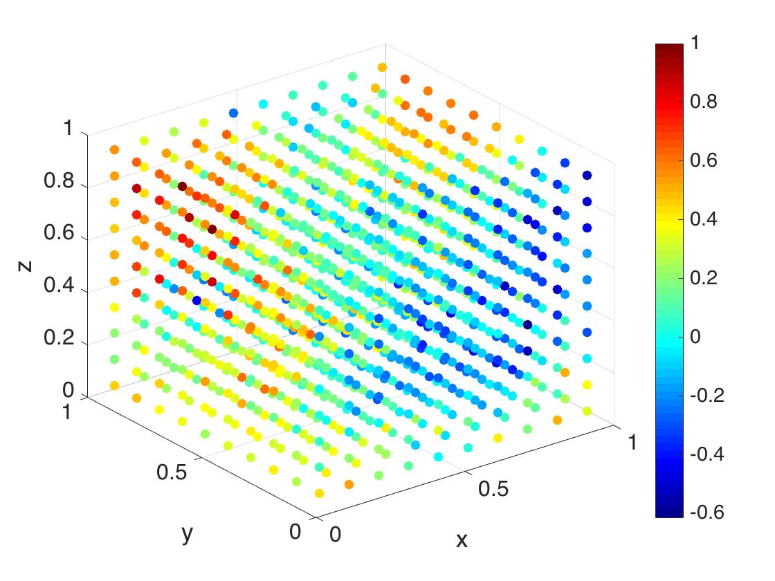
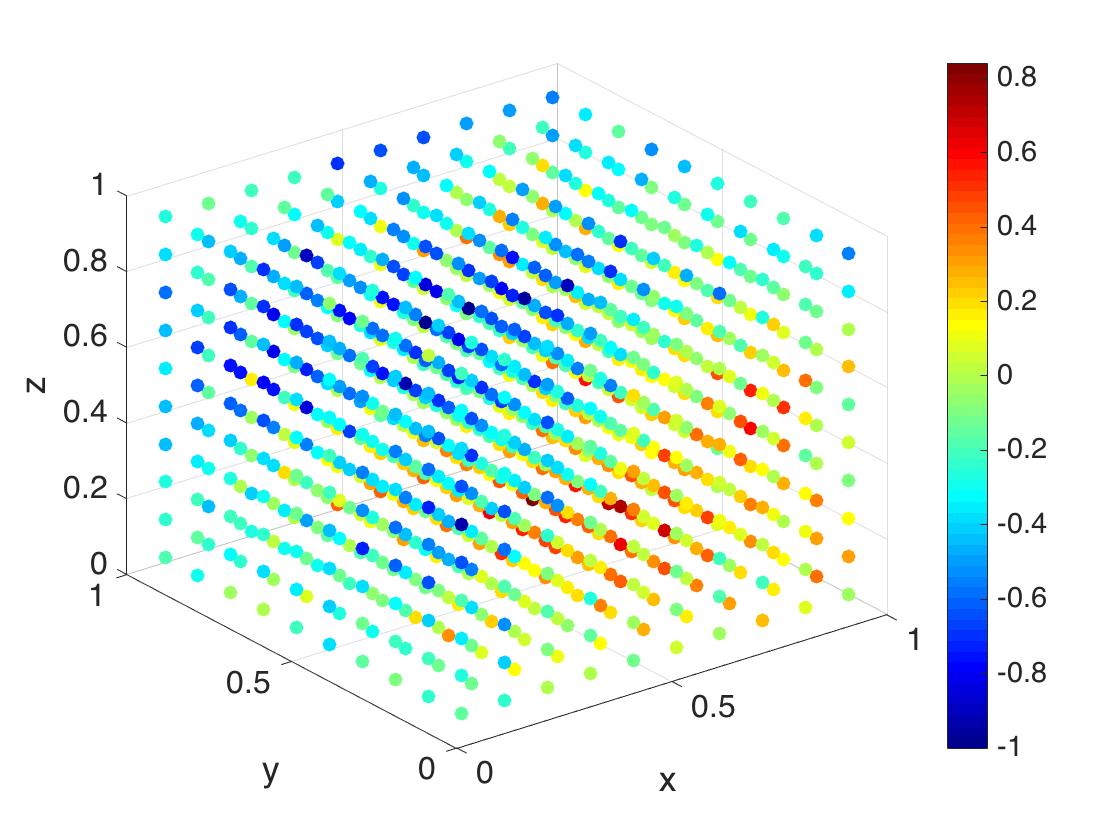
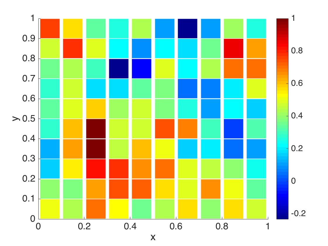
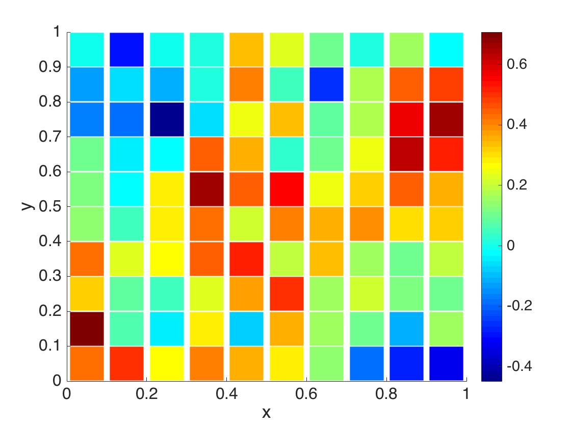
Figure 1: (Above)Samples of the random field $\eta(\omega,\cdot)$ generated using an exponential covariance function with covariance length $\ell=0.5$ on a partition of $D$ parameterized by $h=1/10$. (Below) Cross sections of these samples.

We chose $\varepsilon=$ 0.1, 0.3, 0.5, 0.7, 0.9, and for each fixed $\varepsilon$, Algorithm 2 was used to produce the multi-modes MCIP-DG approximation $\boldsymbol{\Psi}_{N}$ with $N=$ 0, 1, 2, 3, 4, 5, and 6. Figure 2 – 4 demonstrate the behavior of the error $\|\widetilde{\boldsymbol{\Psi}}-\boldsymbol{\Psi}_{N}\|_{L^{2}(D)}$ and $\varepsilon^{N}$ for these tests. These plots use a log-scale for the y-axis for ease of comparison. For all values of $\varepsilon$ tested it is clear that the multi-modes MCIP-DG method produces an accurate approximation in comparison with the standard MCIP-DG method. We also observe that the error converges at a rate $O(\varepsilon^{N})$ as predicted in the previous sections. Surprisingly, we observe the method is working for a large $\varepsilon$ value like $\varepsilon=0.9$. In previous tests involving the multi-modes MCIP-DG method applied to a random Helmholtz problem and random elastic Helmholtz problem the method stopped working for $\varepsilon$ close to 1. See [5, 8]. This is possibly a result of the tests in this paper being carried out with a relatively small wave number parameter $k=2$ and further tests should be carried out to investigate this.

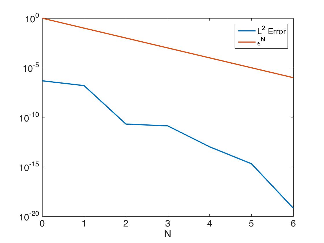
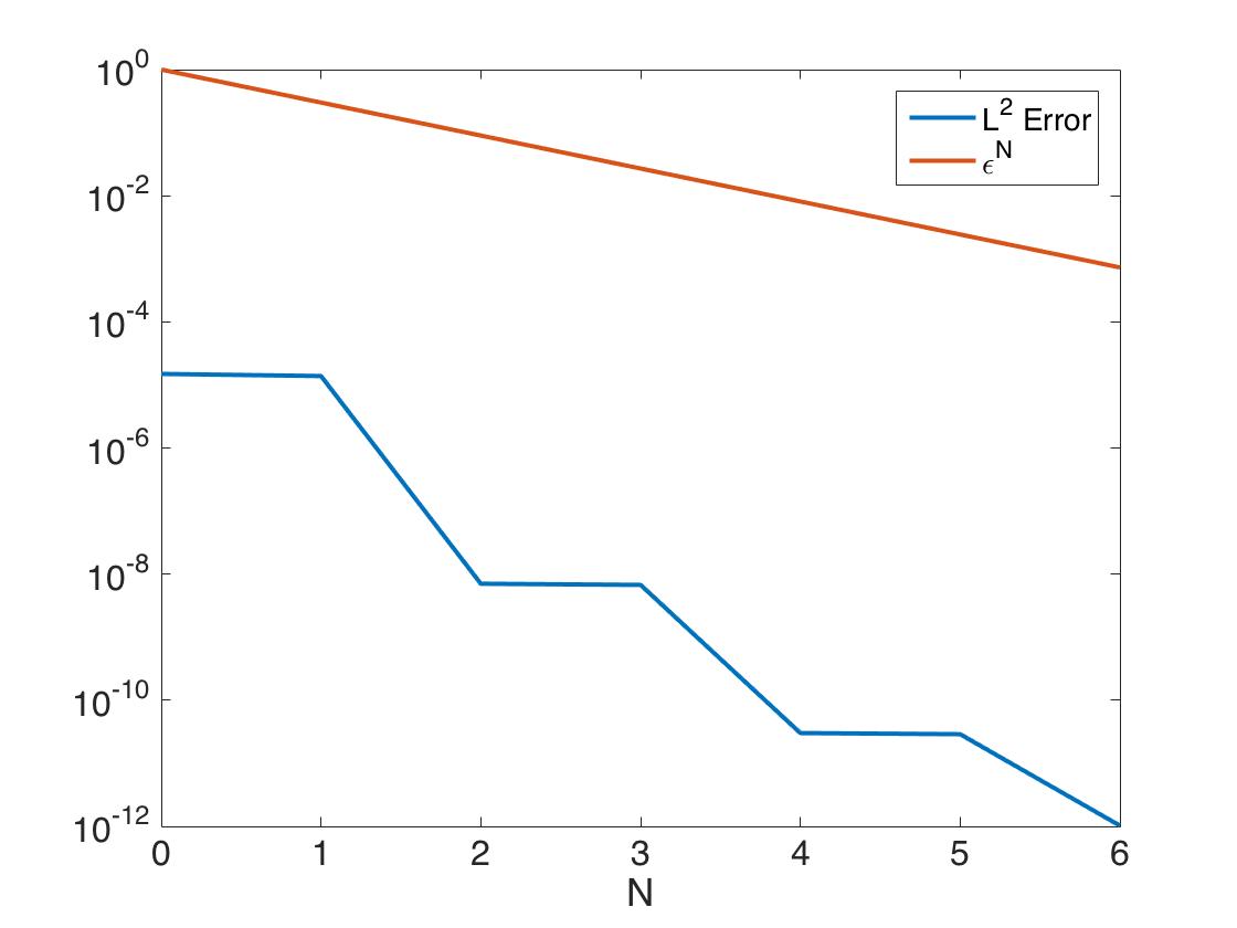
Figure 2: Plots of $\|\widetilde{\boldsymbol{\Psi}}-\boldsymbol{\Psi}_{N}\|_{L^{2}(D)}$ and $\varepsilon^{N}$ with $\varepsilon=0.1$ (Left) and $\varepsilon=0.3$ (Right).

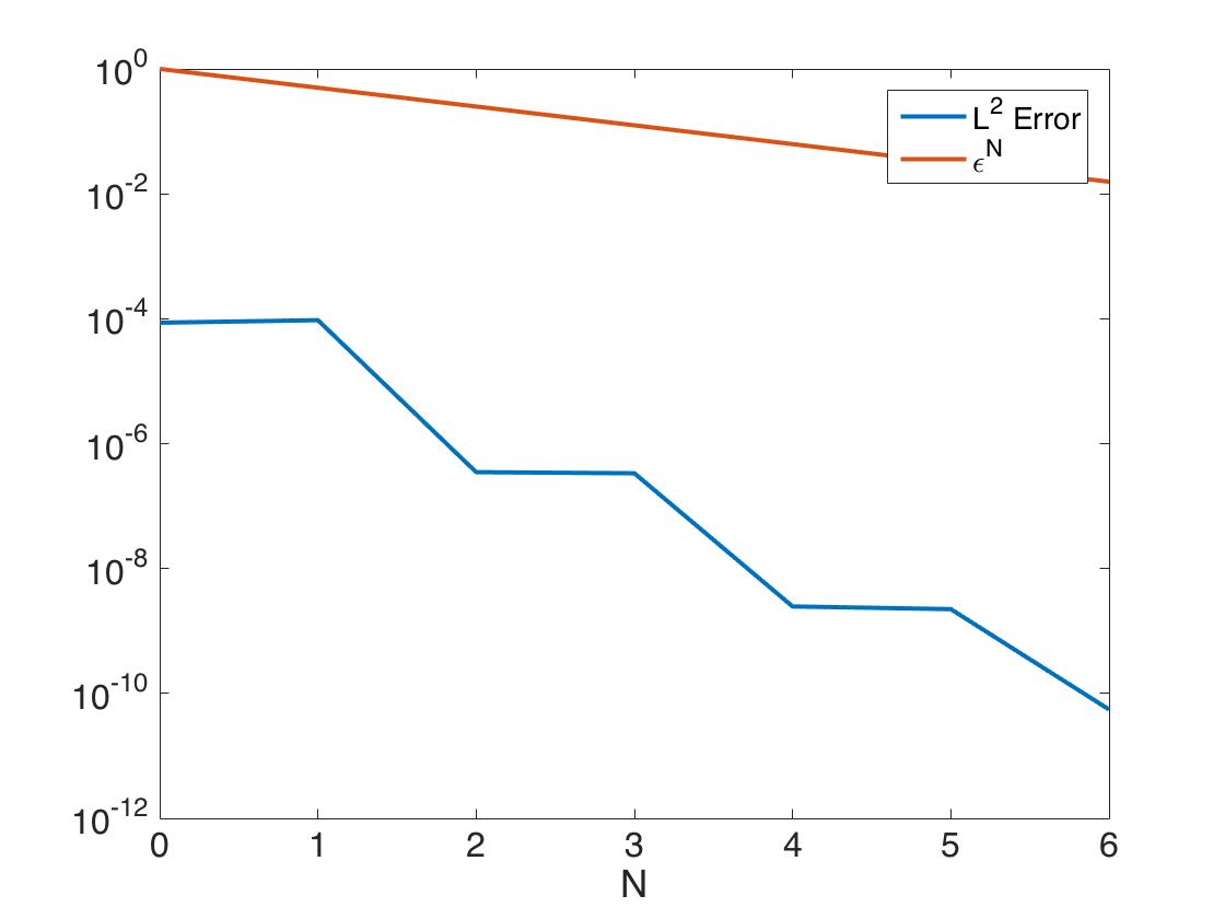
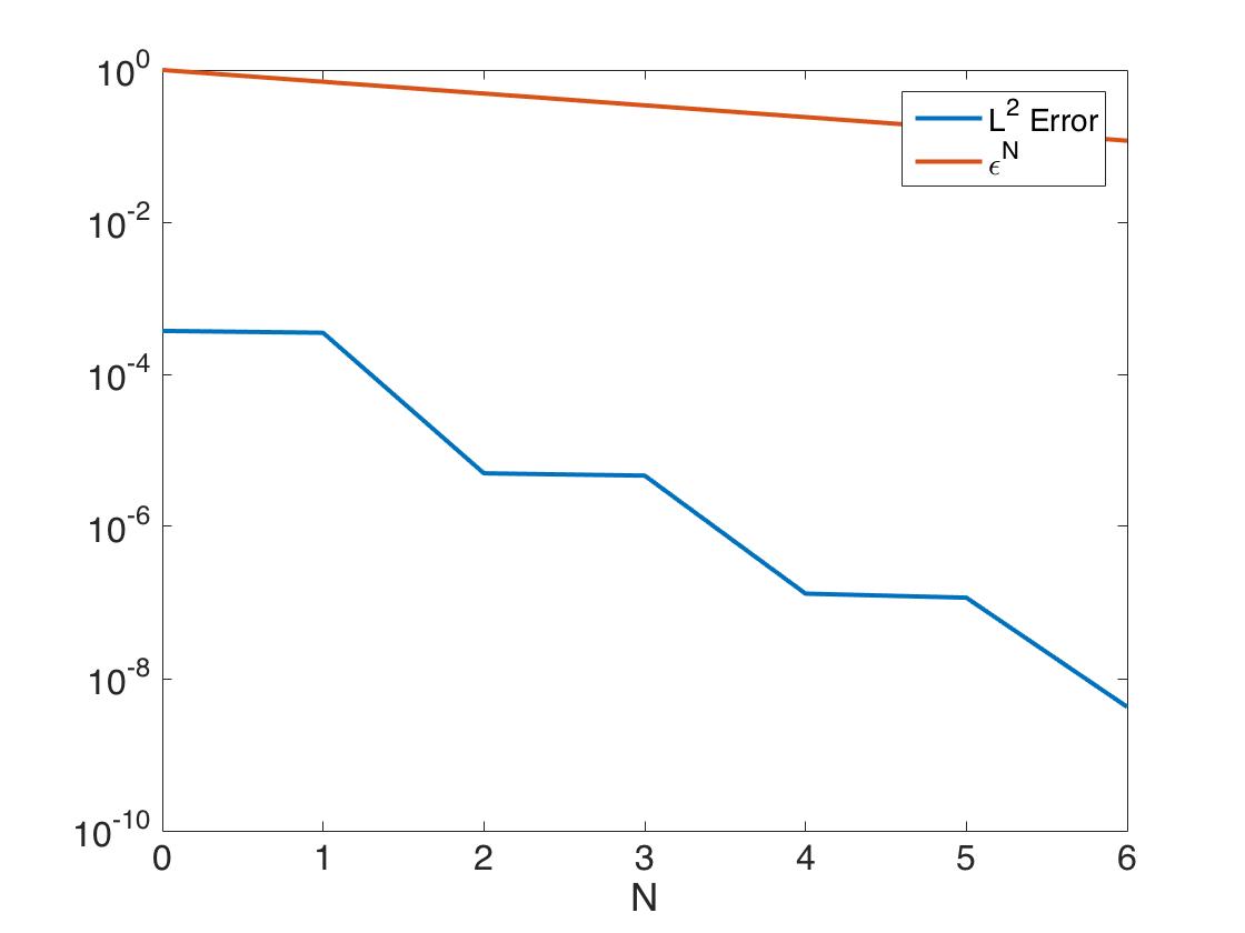
Figure 3: Plots of $\|\widetilde{\boldsymbol{\Psi}}-\boldsymbol{\Psi}_{N}\|_{L^{2}(D)}$ and $\varepsilon^{N}$ with $\varepsilon=0.5$ (Left) and $\varepsilon=0.7$ (Right).

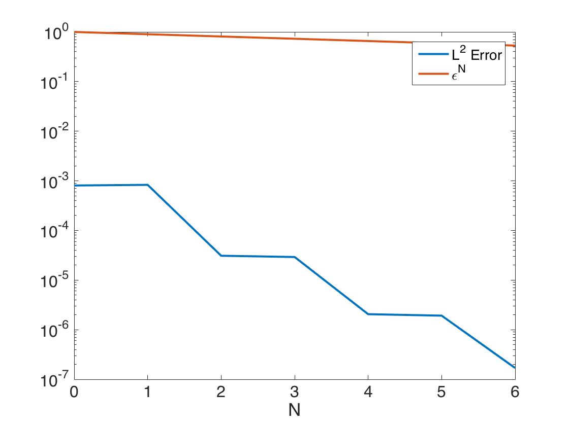
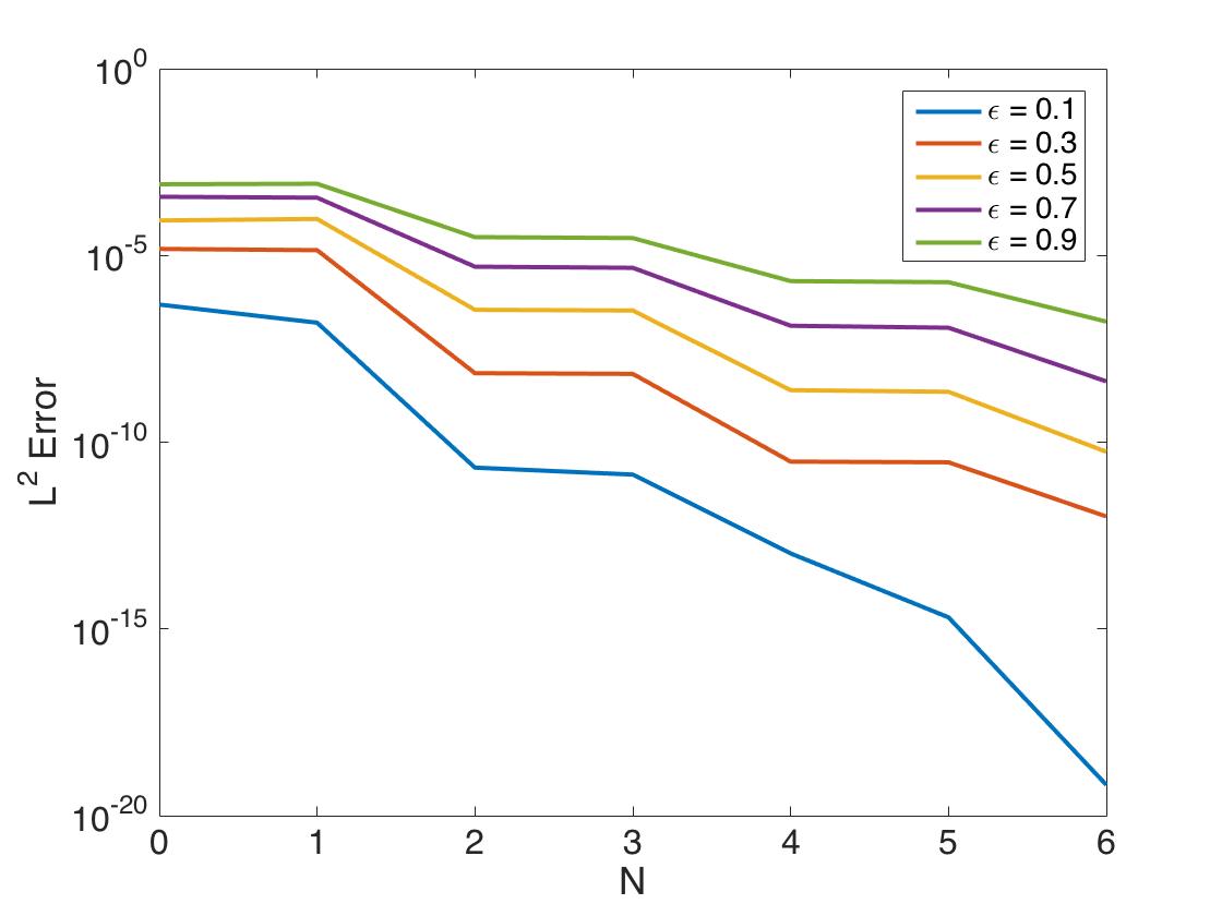
Figure 4: Plot of $\|\widetilde{\boldsymbol{\Psi}}-\boldsymbol{\Psi}_{N}\|_{L^{2}(D)}$ and $\varepsilon^{N}$ with $\varepsilon=0.9$ (Left). Plots of $\|\widetilde{\boldsymbol{\Psi}}-\boldsymbol{\Psi}_{N}\|_{L^{2}(D)}$ for varying values of $\varepsilon$ (Right).

We also observe that the error exhibits a behavior of staying relatively flat for approximations with $N$ odd while decreasing with $N$ even. This behavior was also observed for other Helmholtz-like problems (c.f. [5, 8]). This might lead one to believe that only even-labeled mode functions are useful in the multi-modes approximation, but this would be incorrect since the recursive relationship used to build the multi-modes approximation in (29) involves both odd and even mode functions. From these results it does make more sense to apply the multi-modes MCIP-DG method with $N$ even as it is expected this will result in less error.

We also observe that for $\varepsilon$ small $N$ can be chosen to be relatively small to obtain an accurate approximation. This will lead to great savings in the computation time used to generate the approximation. Table 1 summarizes the computational time used for several modes. As expected the multi-modes MCIP-DG approximation saves a great amount of time in comparison to the standard MCIP-DG approximation. We also observe linear growth in computation time as the number of modes $N+1$ used to generate the approximation increase.

Approximation	CPU Time (s)
$\widetilde{\boldsymbol{\Psi}}$	$41832$
$\boldsymbol{\Psi}_{0}$	$1436.8$
$\boldsymbol{\Psi}_{1}$	$2738.1$
$\boldsymbol{\Psi}_{2}$	$4041.4$
$\boldsymbol{\Psi}_{3}$	$5343$
$\boldsymbol{\Psi}_{4}$	$6647.7$
$\boldsymbol{\Psi}_{5}$	$7953.8$
$\boldsymbol{\Psi}_{6}$	$9261.9$

Table 1: CPU times required to compute the multi-modes MCIP-DG approximation $\boldsymbol{\Psi}_{N}$ and standard MCIP-DG approximation $\widetilde{\boldsymbol{\Psi}}$.

6.2 Numerical experiments with non-smooth random field

This subsection discusses numerical experiments that were carried out using non-smooth random coefficients. In particular, the random coefficient $\eta$ in (1) and the random parameter $\xi$ in (72) were generated by sampling a uniformly distributed random variable for each cube in the partition of $D$ independently. Thus $\eta$ no longer satisfies the condition that it is smooth with $\|\nabla\eta\|_{L^{\infty}(D)}\leq\mu$ a.s. Figure 5 gives two samples of the coefficient functions used in this subsection.

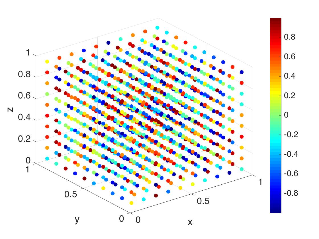
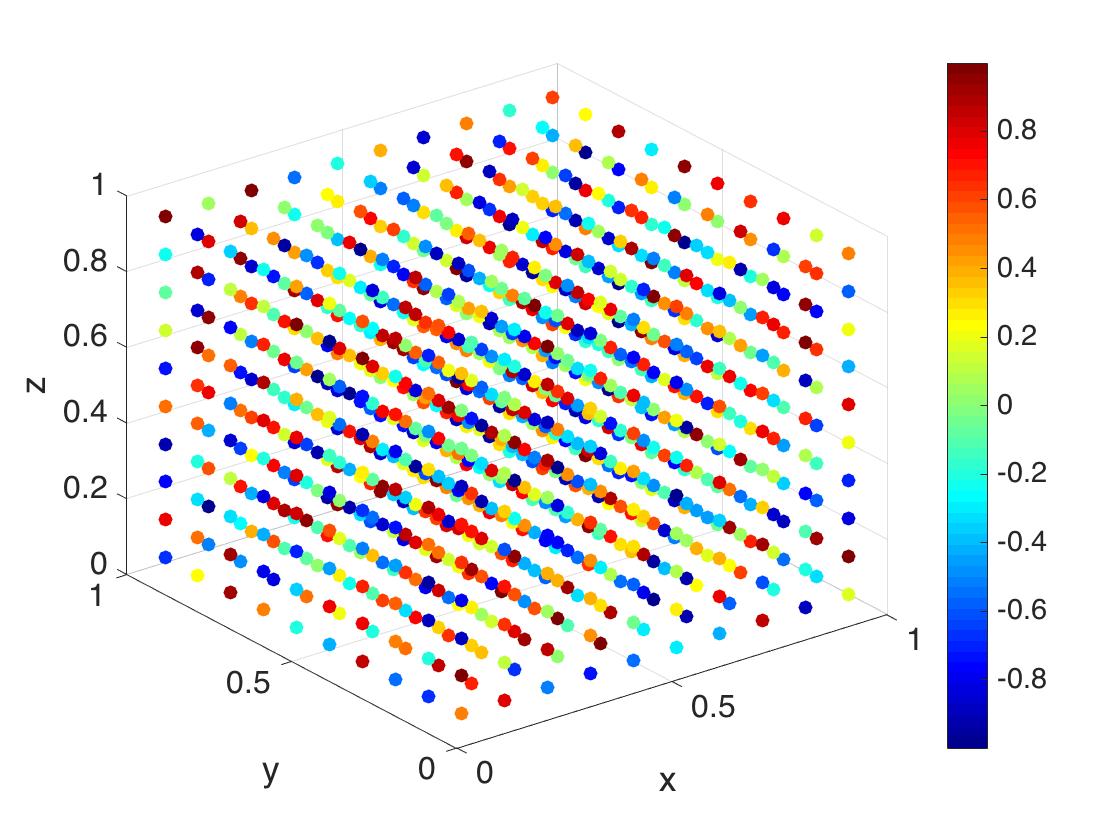
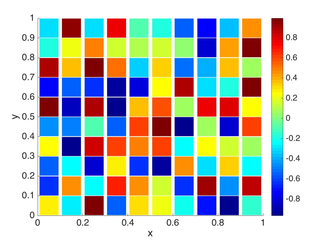
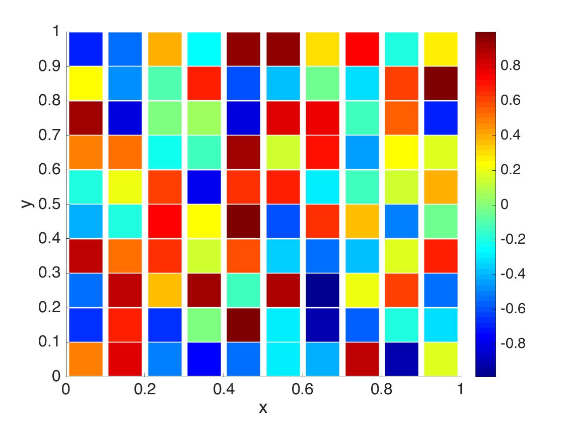
Figure 5: (Above) Samples of the random field $\eta(\omega,\cdot)$ generated using a uniformly distributed random variable for each cube in the partition of $D$ independently. (Below) Cross sections of these samples.

Experiments using non-smooth random coefficients $\eta$ and $\xi$ yielded similar results as demonstrated in Subsection 6.1. In particular, the method still demonstrated an error convergence rate $O(\varepsilon^{N})$ for $\varepsilon$ = 0.1, 0.3, 0.5, 0.7, and 0.9. This is demonstrated in Figure 6.

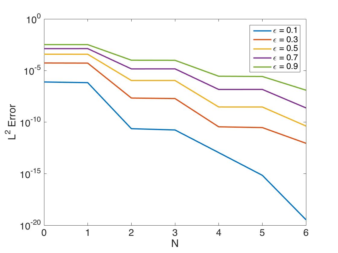
Figure 6: Plots of $\|\widetilde{\boldsymbol{\Psi}}-\boldsymbol{\Psi}_{N}\|_{L^{2}(D)}$ for varying values of $\varepsilon$.

Due to the fact that the experiments with non-smooth random field returned similar convergence results ,we are hopeful that in some cases the added smoothness conditions on the random coefficient $\eta$ may be eliminated. More numerical experiments will be carried out to investigate.

7 Extension to more general random media

To use the multi-modes Monte Carlo DG method we have developed above, it requires that the random media are weak in the sense that the random coefficient $\alpha$ in the PDE has the form $\alpha(\omega,\mathbf{x})=\alpha_{0}+\varepsilon\eta(\omega,\mathbf{x})$ and $\varepsilon$ is not large (note that we have taken $\alpha_{0}=1$ for notational brevity). In this section we present a procedure by which we can extend our multi-modes approach to a class of more general random media.

For general random media, the random coefficient $\alpha$ may not have the required “weak form”. To extend the multi-modes approach presented in the previous section to the general case, our main idea is first to reformulate $\alpha(\omega,\mathbf{x})$ into the desired “weak form” $\alpha_{0}+\varepsilon\eta(\omega,\mathbf{x})$, then to apply the above “weak” field framework. There are at least two ways to do such a reformulation, the first one is to utilize the well-known Karhunen-Loève expansion and the second is to use a stochastic homogenization theory [4]. Since the second approach is more involved and lengthy to describe, below we only outline the first approach.

For many biological and materials science applications, the random media can be described by a Gaussian random field [10, 13, 15]. It is a well-known fact that any Gaussian random field $\alpha$ is uniquely determined by its mean and covariance function. Let $\alpha_{0}(\mathbf{x})$ and $C(\mathbf{x}_{1},\mathbf{x}_{2})$ denote the mean and covariance function of the Gaussian random field $\alpha$, respectively. Two covariance functions, which are widely used in geoscience and materials science, are $C(\mathbf{x}_{1},\mathbf{x}_{2})=\exp(-|\mathbf{x}_{1}-\mathbf{x}_{2}|^{m}/\ell)$ for $m=1,2$ and $0<\ell<1$ (cf. [15, Chapter 7]). Here $\ell$ is called correlation length which determines the range (or frequency) of the noise. We now recall that the Karhunen-Loève expansion for $\alpha(\omega,\mathbf{x})$ takes the following form (cf. [15]):

$$\alpha(\omega,\mathbf{x})=\alpha_{0}(\mathbf{x})+\sum_{k=1}^{\infty}\sqrt{\lambda_{k}}\phi_{k}(\mathbf{x})\xi_{k}(\omega),$$

where $\{(\lambda_{k},\phi_{k})\}_{k\geq 1}$ is the eigenset of the (self-adjoint) covariance operator and $\{\xi_{k}\sim N(0,1)\}_{k\geq 1}$ are i.i.d. random variables. It can be shown that $\lambda_{k}=O(\ell^{r})$ for some $r>1$ depending on the spatial domain $D$ in which the PDE is defined (cf. [15, Chapter 7]). Consequently, for random media with small correlation length $\ell$, we have

$$\alpha(\omega,\mathbf{x})=\alpha_{0}(\mathbf{x})+\sqrt{\lambda_{1}}\zeta(\omega,\mathbf{x}),\qquad\zeta(\omega,\mathbf{x}):=\sum_{k=1}^{\infty}\sqrt{\frac{\lambda_{k}}{\lambda_{1}}}\,\phi_{k}(\mathbf{x})\xi_{k}(\omega),$$

Thus, setting $\varepsilon=\sqrt{\lambda_{1}}=O(\ell^{\frac{r}{2}})$ then leads to $\alpha(\omega,x)=\alpha_{0}+\varepsilon\zeta$, which has the desired “weak form” which is given by a sum of a deterministic field and a small random perturbation. As a result, our multi-modes Monte Carlo DG method is now applicable.

We like to note that the classical Karhunen-Loève expansion may be replaced by other types of expansion formulas which may result in more efficient multi-modes Monte Carlo methods. The feasibility and competitiveness of non-Karhunen-Loève expansion techniques will be investigated in a forthcoming work, where comparison among different expansion choices will also be studied. Finally, we remark that the DG method can be replaced by any other space discretization method such as finite difference, finite element, and spectral methods in the main algorithm.

References

• [1] L. Andrews and R. Phillips. Laser beam propagation through random media. Bellingham, WA: SPIE press, 2005.
• [2] I. Babuška, R. Tempone, and G.E. Zouraris. Galerkin finite element approximations of stochastic elliptic partial differential equations. SIAM J. Numer. Anal., 42:800 – 825, 2004.
• [3] D. Colton and R. Kress. Inverse Acoustic and Electromagnetic Scattering Theory. Springer-Verlag, Berlin, 1992.
• [4] M. Duerinckx, A. Gloria, and F. Otto. The structure of fluctuations in stochastic homogenization. arXiv:1602.01717[math.AP].
• [5] X. Feng, J. Lin, and C. Lorton. An efficient numerical method for acoustic wave scattering in random media. SIAM/ASA J. UQ, 3:790 – 822, 2015.
• [6] X. Feng, J. Lin, and C. Lorton. A multi-modes Monte Carlo finite element method for elliptic partial differential equations with random coefficients. Int. J. Uncertain. Quantif., 6(5):429 – 443, 2016.
• [7] X. Feng, J. Lin, and D. Nicholls. An efficient Monte Carlo-transformed field expansion method for electromagnetic wave scattering by random rough surface. Commun. Comput. Phys., 23:685–705, 2018.
• [8] X. Feng and C. Lorton. An efficient Monte Carlo interior penalty discontinuous Galerkin method for elastic wave scattering in random media. Comput. Methods Appl. Mech. Engrg., 315:141 – 168, 2017.
• [9] X. Feng and H. Wu. An absolutely stable discontinuous Galerkin method for the indefinite time-harmonic Maxwell equations with large wave number. SIAM J. Numer. Anal., 52:2356 – 2380, 2014.
• [10] J. Fouque, J. Garnier, G. Papanicolaou and K. Solna, Wave Propagation and Time Reversal in Randomly Layered Media, Stoch. Model. and Applied Prob., Vol. 56, Springer, 2007.
• [11] D. Gilbarg and N.S. Trudinger, Elliptic Partial Differential Equations of Second Order, Classics in Mathematics, Springer-Verlag, 2001; reprint of the 1998 edition.
• [12] R. Hiptmair, A. Moiola, and I. Perugia. Error analysis of Trefftz-discontinuous Galerkin methods for the time-harmonic Maxwell equations. Math. Comp., 82:247 – 268, 2013.
• [13] A. Ishimaru. Wave Propagation and Scattering in Random Media. New York: Academic press, 1978.
• [14] K. Liu and B. Rivière. Discontinuous Galerkin methods for elliptic partial differential equations with random coefficients. Int. J. Computer Math., 90(11):2477 – 2490, 2013.
• [15] G. Lord, C. Powell, and T. Shardlow. An Introduction to Computational Stochastic PDEs. Cambridge University Press, 2014.
• [16] C. Lorton. Numerical methods and algorithms for high frequency wave scattering problems in homogeneous and random media. PhD thesis, The University of Tennessee, August 2014.
• [17] P. Monk. Finite Element Methods for Maxwell’s Equations. Oxford University Press, New York, 2003.
• [18] L. Tsang, J. Kong, and R. Shin. Theory of microwave remote sensing. New York: Wiley-Interscience, 1985.