Learning to Communicate in UAV-aided Wireless Networks: Map-based Approaches

Abstract

We consider a scenario where an UAV-mounted flying base station is providing data communication services to a number of radio nodes spread over the ground. We focus on the problem of resource-constrained UAV trajectory design with (i) optimal channel parameters learning and (ii) optimal data throughput as key objectives, respectively. While the problem of throughput optimized trajectories has been addressed in prior works, the formulation of an optimized trajectory to efficiently discover the propagation parameters has not yet been addressed. When it comes to the communication phase, the advantage of this work comes from the exploitation of a 3D city map. Unfortunately, the communication trajectory design based on the raw map data leads to an intractable optimization problem. To solve this issue, we introduce a map compression method that allows us to tackle the problem with standard optimization tools. The trajectory optimization is then combined with a node scheduling algorithm. The advantages of the learning-optimized trajectory and of the map compression method are illustrated in the context of intelligent IoT data harvesting.

I Introduction

The use of unmanned aerial vehicles (UAVs) also known as drones as base stations (BSs) in future wireless communication networks is currently gaining significant attention for its ability to yield ultra-flexible deployments, in use cases ranging from disaster recovery scenarios, coverage of flash-crowd events, and data harvesting in IoT applications [1, 2, 3].

Several new and fascinating issues arise from the study of flying BSs in a wireless network. These can be broadly categorized into placement and path planning problems. While placement problem deals with finding flexible yet static locations of the UAV BSs, path planning involves finding UAV trajectories. In both cases the aim is to optimize metrics like throughput, network coverage, energy efficiency, etc., [4, 5, 6, 7, 8, 9, 10, 11, 12, 13, 14].

When it comes to placement or trajectory design problems, most existing solutions rely on simplified channel attenuation models which are based on either (deterministically guaranteed) line-of-sight (LoS) links [8, 9, 10, 11, 14, 13, 12], or predictive models for the probability of occurrence of a LoS link [6, 7, 4, 5]. In the latter approach, a global statistical model predicts the LoS availability as a function of, e.g., UAV altitude and distance to the user. The advantage of the global statistical LoS model lies in its simplicity for system analysis. However, it lacks actual performance guarantees for either placement or trajectory design algorithms when used in a real-life navigation scenario. The key reason for this is that, the local terrain topology may sharply differ from the predictions drawn from statistical features. In order to circumvent this problem, the embedding of actual 3D city map data in the UAV placement algorithms has been recently proposed [8, 7]. Map-based approaches help providing a reliable prediction of LoS availability for any pair of UAV and ground node locations, hence lead to improved performance guarantees. However, the gain comes at the expense of computational and memory costs related to processing of the map data. So far, map-based approaches have been investigated mainly for static UAV placement [8, 9, 7]. In many scenarios, including IoT data harvesting, there is an interest in flying along a path that brings the UAV-mounted BS closer to each and every ground node. However, to the best of our knowledge, none of the previous works have considered the crucial advantage of exploiting 3D map data in communication-oriented UAV trajectory design.

Another common assumption in previous works is that the channel model parameters are assumed to be known when designing the UAV trajectory. However, in reality these parameters need to be learned based on the measurements collected from the ground users. As a result, an important question arises: What is an efficient way of collecting radio measurements by the UAV from the ground users in order to estimate the channel model parameters?

In this work, we consider an instance of IoT data harvesting scenario where an UAV flies over a city endowed with a number of scattered ground nodes (e.g. radio-equipped sensors). We then formulate a resource-constrained UAV trajectory design problem in order to optimize data throughput from the ground nodes while capitalizing on 3D map data. Since the data communication phase critically depends on the knowledge of radio channel parameters, we also formulate a novel optimal trajectory design problem from a parameter learning point of view. Specifically, our contributions are as follows:

• We formulate and solve a learning trajectory optimization problem in order to minimize the estimation error of the channel model parameters. The devised trajectory allows the UAV to exploit the map and quickly learn the propagation parameters.

• Based on the learned parameters, we formulate a joint trajectory and node scheduling problem which allows us to maximize the traffic communicated from each node to the UAV in a fair manner. An iterative algorithm is proposed to solve the optimization problem. It is shown that the algorithm converges at least to a local optimal solution. While the algorithm exploits the possibly rich map data, it does so via a map compression method which renders the trajectory optimization problem differentiable and amenable to standard optimization tools, hence mitigating a known drawback of map-based approaches.

Note that, the proposed map-compression method allows us to smooth out the map data while preserving the node location-dependent channel behavior around that node. The gains brought by the exploitation of 3D map data are illustrated, in both channel parameters learning and the communication problem, in the context of an urban IoT scenario.

This paper is organized as follows: Section II introduces the system model. In Section III, we formulate and solve the problem of learning trajectory optimization. In Section IV, we formulate the joint communication trajectory and node scheduling optimization problem whose solution is provided in Section V. Numerical results are presented in Section VI to validate the performance of the proposed algorithms. Finally, Section VII concludes the paper with some perspectives.

Notation: Matrices are represented by uppercase bold letters, vectors are represented by lowercase bold letters. The transpose of matrix $\mathbf{A}$ is denoted by $\mathbf{A}^{\text{T}}$. The trace and determinant of matrix $\mathbf{A}$ are denoted by $\text{tr}[\mathbf{A}]$ and $\text{det[}\mathbf{A}]$, respectively. The set of integers from $m$ to $n$, $m<n$, is represented by $[m,\,n]$. The expectation operator is denoted by $\text{E}[.]$.

II SYSTEM MODEL

A wireless communication system where an UAV-mounted flying BS serving $K$ static ground level nodes (IoT sensors, radio terminals, etc.) in an urban area is considered. The $k$-th ground node, $k\in\left[1,K\right]$, is located at ${\bf u}_{k}=[x_{k},y_{k},0]^{\text{T}}\in\mathbb{R}^{3}.$ By no means the ground level node assumption is restrictive, the proposed algorithms in this work can in principle be applied to a scenario where the nodes are located in 3D. The UAV’s mission consists of a learning phase which is of duration $T_{l}$ and then followed by a communication phase of duration $T_{c}$. During the learning phase, the UAV estimates the propagation parameters of the environment by collecting the radio measurements from the ground users. These estimates are then exploited in the communication phase to optimally serve the ground nodes. Note that in this paper, we are treating the learning and the communication phases that are separated in time. This allows us to obtain optimal trajectories for both phases independently, i.e., if one is only interested in learning or communication scenario this solution serves the purpose. The joint channel learning and communication trajectory design is appealing yet a challenging problem and is left for future work. Whether be it in learning or communication phase, the time-varying coordinate of the UAV/drone is denoted by ${\bf v}(t)=[x(t),y(t),z(t)]^{\text{T}}\in\mathbb{R}^{3}$, where $z(t)$ represents the altitude of the drone.

For the ease of exposition, we assume that the time period $T_{l}$ and $T_{c}$ are discretized into $N_{l}$ and $N_{c}$ equal-time slots, respectively. The time slots are chosen sufficiently small such that the UAV’s location, velocity, and channel gains can be considered to remain constant in one slot. Hence, the UAV’s position ${\bf v}(t)$ is approximated by a sequence

$${\bf v}[n]=[x[n],y[n],z[n]]^{\text{T}},\leavevmode\nobreak\ n\in[1,N_{l}]\ \mbox{(or) }n\in[1,N_{c}].$$ (1)

We assume that the ground nodes and the drone are equipped with GPS receivers, hence the coordinates ${\bf u}_{k},\forall k$ and ${\bf v}[n],\leavevmode\nobreak\ n\in[1,N_{l}]\ \mbox{(or) }n\in[1,N_{c}]$ are known.

II-A Channel Model

In this section, we describe the channel model that is used for computing the channel gains between the UAV and the ground users. The model parameters are estimated in the learning phase from the collected radio measurements. Classically, the channel gain between two radio nodes which are separated by distance $d$ meters is modeled as[15, 16]

$$\gamma_{s}=\frac{\beta_{s}}{d^{\alpha_{s}}}\times\xi_{s},$$ (2)

where $\alpha_{s}$ is the path loss exponent, $\beta_{s}$ is the average channel gain at the reference point $d=1$ meter, $\xi_{s}$ denotes the shadowing component, and finally $s\in\left\{\lx@glossaries@gls@link{acronym}{los}{\leavevmode\text{LoS}},\text{NLoS}\right\}$ emphasizes the strong dependence of the propagation parameters on LoS or non-line-of-sight (NLoS) scenario. Note that (2) represents the channel gain which is averaged over the small scale fading of unit variance. The channel gain in dB can be written as

$$g_{s}=\ss{}_{s}-\alpha_{s}\varphi(d)+\eta_{s},$$ (3)

where $g_{s}=10\log_{10}\gamma_{s},\ss_{s}=10\log_{10}\beta_{s},\varphi(d)=10\log_{10}\left(d\right)$, $\eta_{s}=10\log_{10}\xi_{s}$, and $\eta_{s}$ is modeled as a Gaussian random variable with $\mathcal{N}(0,\sigma_{s}^{2})$.

II-B UAV Model

During the mission, drone’s position evolves according to

$${\bf v}[n+1] ={\bf v}[n]+\left[\begin{array}[]{c}\cos\left(\phi[n]\right)\cos\left(\psi[n]\right)\\ \sin\left(\phi[n]\right)\cos\left(\psi[n]\right)\\ \sin\left(\psi[n]\right)\end{array}\right]\rho[n]\,,$$ (4d)

$$h_{min}\leq z[n]\leq h_{max},\ \forall n\in[1,N_{l}-1]\ \mbox{(or) }n\in[1,N_{c}-1],$$ (4e)

where in the $n$-th time slot, $0\leq\rho[n]\leq\rho_{max}$ represents the distance traveled by the drone, $0\leq\phi[n]\leq 2\pi$ and $-\frac{\pi}{2}\leq\psi[n]\leq\frac{\pi}{2}$ represent the heading and elevation angles, respectively. The maximum distance traveled in a time slot is denoted by $\rho_{max}$ and it depends on the maximum velocity. The constraint (4e) reflects the fact that the drone always flies at an altitude higher than $h_{min}$ and lower than $h_{max}$, with $h_{min}$ being the height of the tallest building in the city.

III Learning Trajectory Design

In this section, our goal is to find the UAV trajectory, over which the channel measurements are collected from the ground nodes, that results in the minimum estimation error of the channel model parameters. While the problem of learning the channel parameters from a pre-determined measurement data set has been addressed in the prior literature [16, 17], the novelty of our work lies in the concept of optimizing the flight trajectory itself so as to accelerate the learning process. The channel measurement collection and learning process are described next.

III-A Measurement Collection and Channel Learning

In the learning phase, the measurement harvesting is performed over an UAV trajectory that starts at a base position ${\bf x}_{b}\in\mathbb{R}^{3}$ and ends at a terminal position ${\bf x}_{t}\in\mathbb{R}^{3}$. Mathematically,

$${\bf v}[1]={\bf x}_{b},\leavevmode\nobreak\ {\bf v}[N_{l}]={\bf x}_{t}.$$ (5)

The base position is typically the take-off base for the UAV while ${\bf x}_{t}$ can be selected in different ways, including ${\bf x}_{t}={\bf x}_{b}$ (loop) or as a location where the communication services are to begin right after the learning phase. In the $n$-th time interval, $n\in[1,N_{l}]$, the measurements collected from the ground nodes can be written as

$${\bf g}_{s,n}=\left[g_{s,1},g_{s,2},\cdots,g_{s,\delta_{s,n}}\right]^{\text{T}},$$

where $g_{s,i}^{\text{ }}$ is the channel gain of the $i$-th measurement, $i\in[1,\delta_{s,n}]$, and $\delta_{s,n}$ is the number of measurements obtained for the propagation segment group $s\in\{\text{LoS},\text{NLoS}\}$. For the LoS/NLoS classification of the measurements, we leverage the knowledge of a 3D city map [18]. Based on such map, we can predict LoS (un)availability on any given UAV-ground nodes link from a trivial geometry argument: For a given UAV position, the ground node is considered in LoS to the UAV if the straight line passing through the UAV’s and the ground node’s position lies higher than any buildings in between.

Using (3), the $i$-th measurement can be modeled as

$$g_{s,i}^{\text{ }}={\bf{\bf a}}_{s,i}^{\text{T}}\,{\bf\boldsymbol{\omega}}_{s}+\eta_{s,i}^{\text{ }},$$ (6)

where ${\bf a}_{s,i}=[-\varphi(d_{i}),\,1]^{\text{T}}$ with $d_{i}$ being the distance between the drone and ground node in the $i$-th measurement, ${\bf\boldsymbol{\omega}}_{s}=[\alpha_{s},\,\ss_{s}]^{\text{T}}$ is the vector of channel parameters, and $\eta_{s,i}$ denotes the shadowing component in the $i$-th measurement. The measurements collected in the $n$-th interval can now be written as

$$\mathbf{g}_{s,n}={\bf A}_{s,n}\,{\bf\boldsymbol{\omega}}_{s}+\boldsymbol{\eta}_{s,n},$$ (7)

where ${\bf A}_{s,n}=\left[{\bf a}_{s,1},\cdots,{\bf a}_{s,\delta_{s,n}}\right]^{\text{T}},\,\boldsymbol{\eta}_{s,n}=[\eta_{s,1}^{\text{ }},\cdots,\eta_{s,\mathcal{\delta}_{s,n}}^{\text{ }}]^{\text{T}}$. Finally, we stack up the measurements gathered by the drone up to time step $n$ as

$${\bf\bar{\mathbf{g}}}_{s,n}={\bf\bar{A}}_{s,n}\,{\bf\boldsymbol{\omega}}_{s}+\boldsymbol{\bar{\eta}}_{s,n},$$ (8)

where ${\bf{\bf\bar{\mathbf{g}}}}_{s,n}=\left[\mathbf{g}_{s,1}^{\text{T}},\cdots,\mathbf{g}_{s,n}^{\text{T}}\right]^{\text{T}},{\bf\bar{A}}_{s,n}=\left[{\bf A}_{s,1}^{\text{T}},\cdots,{\bf A}_{s,n}^{\text{T}}\right]^{\text{T}},\,\text{and }\boldsymbol{\bar{\eta}}_{s,n}=\left[\boldsymbol{\eta}_{s,1}^{\text{T}},\cdots,\boldsymbol{\eta}_{s,n}^{\text{T}}\right]^{\text{T}}$.

Assuming that the measurements collected over a trajectory are independent, the maximum likelihood estimation of ${\bf\boldsymbol{\omega}}_{s},s\in\{\text{LoS},\text{NLoS}\}$ based on the measurements collected up to time step $n$ is given by [16, 18]

$$\hat{\boldsymbol{\omega}}_{s,n}=\left({\bf\bar{A}}_{s,n}^{\text{T}}\,{\bf\bar{A}}_{s,n}\right)^{-1}{\bf\bar{A}}_{s,n}^{\text{T}}\,{\bf\bar{\mathbf{g}}}_{s,n}.$$ (9)

By substituting (8) in (9), we obtain

$$\hat{\boldsymbol{\omega}}_{s,n}-\boldsymbol{\omega}_{s}=\left({\bf\bar{A}}_{s,n}^{\text{T}}\,{\bf\bar{A}}_{s,n}\right)^{-1}{\bf\bar{A}}_{s,n}^{\text{T}}\boldsymbol{\bar{\eta}}_{s,n}.$$ (10)

Since $\hat{\boldsymbol{\omega}}_{s,n}$ is unbiased, the mean squared error of the estimated parameters can be obtained as [19]

$$\text{E}\left\|\hat{\boldsymbol{\omega}}_{s,n}-\boldsymbol{\omega}_{s}\right\|^{2} =\text{tr}\left[Cov\left\{\hat{\boldsymbol{\omega}}_{s,n}\right\}\right]$$

$$=\sigma_{s}^{2}\,\text{tr}\left[\left({\bf\bar{A}}_{s,n}^{\text{T}}\,{\bf\bar{A}}_{s,n}\right)^{-1}\right].$$ (11)

Let

$$e_{s}[n]\triangleq\text{tr}\left[\left({\bf\bar{A}}_{s,n}^{\text{T}}\,{\bf\bar{A}}_{s,n}\right)^{-1}\right],$$

and assuming that $\sigma_{\lx@glossaries@gls@link{acronym}{nlos}{\leavevmode\text{NLoS}}}^{2}=\kappa\cdot\sigma_{\lx@glossaries@gls@link{acronym}{los}{\leavevmode\text{LoS}}}^{2},\,\kappa\geq 1$ [20], the total estimation error in both propagation segments is given by

$$\sum_{s}\text{E}\left\|\hat{\boldsymbol{\omega}}_{s,n}-\boldsymbol{\omega}_{s}\right\|^{2}=\sigma_{\lx@glossaries@gls@link{acronym}{los}{\leavevmode\text{LoS}}}^{2}\left(e_{\lx@glossaries@gls@link{acronym}{los}{\leavevmode\text{LoS}}}[N_{l}]+\kappa\,e_{\lx@glossaries@gls@link{acronym}{nlos}{\leavevmode\text{NLoS}}}[N_{l}]\right).$$ (12)

Note that a full rank ${\bf\bar{A}}_{s,n}$ is assumed in calculating the error for both LoS and NLoS categories over the course of the trajectory. If there are not enough measurements in a particular segment by the end of the trajectory, the estimation error is assigned as infinity in that segment.

III-B Optimization Problem

The optimal learning trajectory that minimizes the estimation error can be formulated as

$$\min_{\Phi,\Psi,\mathcal{R}}\ e_{\lx@glossaries@gls@link{acronym}{los}{\leavevmode\text{LoS}}}[N_{l}]+\kappa\,e_{\lx@glossaries@gls@link{acronym}{nlos}{\leavevmode\text{NLoS}}}[N_{l}]$$ (13a)

s.t. $$\eqref{eq:DroneDyn},\,\eqref{eq:LearnBoundCond}$$ (13b)

where $\Phi,\Psi,$ and $\mathcal{R}$ are defined as

$$\Phi =\left\{0\leq\phi[n]<2\pi,\,n\in[1,N_{l}-1]\right\},$$

$$\Psi =\left\{-\frac{\pi}{2}\leq\psi[n]\leq\frac{\pi}{2},\,n\in[1,N_{l}-1]\right\},$$

$$\mathcal{R} =\left\{0\leq\rho[n]\leq\rho_{max},\,n\in[1,N_{l}-1]\right\}.$$

As the estimation error depends on the matrix ${\bf\bar{A}}_{s,N_{l}}$ which has a very complicated expression in terms of $\phi[n],\psi[n],$ and $\rho[n]$, it is hard to obtain an analytical solution for problem (13) in general. Therefor, we tackle (13) by discretizing the optimization variables and then employing dynamic programming (DP) [21] to find the solution. To apply DP, the estimation error $e_{s}[N_{l}]$ needs to be rewritten as follows

$$e_{s}[N_{l}] =\text{tr}\left[\left(\left[\begin{array}[]{c}{\bf\bar{A}}_{s,N_{l}-1}\\ {\bf A}_{s,N_{l}}\end{array}\right]^{\text{T}}\,\left[\begin{array}[]{c}{\bf\bar{A}}_{s,N_{l}-1}\\ {\bf A}_{s,N_{l}}\end{array}\right]\right)^{-1}\right]$$ (18)

$$\overset{(a)}{=}e_{s}[N_{l}-1]-r_{s}[N_{l}]$$

$$\overset{(b)}{=}e_{s}[1]-\sum_{n=2}^{N_{l}}r_{s}[n],$$ (19)

where we denote $r_{s}[n]$ as the amount of improvement in the estimate within time slot $n$, and it is given by

$$r_{s}[n]=\text{tr}\left[{\bf H}_{s,n}\,{\bf A}_{s,n}^{\text{T}}\left({\bf I}+{\bf A}_{s,n}\,{\bf H}_{s,n}\,{\bf A}_{s,n}^{\text{T}}\right)^{-1}\,{\bf A}_{s,n}\,{\bf H}_{s,n}\right],$$ (20)

${\bf H}_{s,n}\triangleq\left({\bf\bar{A}}_{s,n-1}^{\text{T}}\,{\bf\bar{A}}_{s,n-1}\right)^{-1}$, ${\bf I}$ is the identity matrix, (a) follows from the matrix inversion lemma, and (b) follows from the recursive relation. Now (13) can be reformulated as

$$\min_{\Phi,\Psi,\mathcal{R}}\ \sum_{n=1}^{N_{l}}\tilde{e}_{\lx@glossaries@gls@link{acronym}{los}{\leavevmode\text{LoS}}}[n]+\kappa\,\tilde{e}_{\lx@glossaries@gls@link{acronym}{nlos}{\leavevmode\text{NLoS}}}[n]$$ (21a)

s.t. $$\eqref{eq:DroneDyn},\,\eqref{eq:LearnBoundCond}$$ (21b)

where

$$\tilde{e}_{s}[n]=\begin{cases}e_{s}[1]&n=1\\ -r_{s}[n]&n\in[2,N_{l}]\end{cases}.$$

III-C Dynamic Programming

To solve (21) by DP, we constraint (and thus approximate) the possible drone locations and the optimization variables to a limited alphabet and then use Bellman’s recursion to compute the optimal discrete trajectory. We start by introducing some notations.

Let ${\bf v}[n],\,n\in[1,N_{l}]$ denotes the states and $\boldsymbol{\pi}[n]=\left[\phi[n],\psi[n],\rho[n]\right]^{\text{T}}$ represents the input action at time $n\in[1,N_{l}-1]$ such that

$$\phi[n] \in\left\{0,\frac{\pi}{4},\frac{\pi}{2},\frac{3\pi}{4},\pi,\frac{5\pi}{4},\frac{3\pi}{2},\frac{7\pi}{4}\right\},$$

$$\psi[n] \in\left\{-\frac{\pi}{2},-\frac{\pi}{4},0,\frac{\pi}{4},\frac{\pi}{2}\right\},$$

$$\rho[n] \in\left\{0,a_{h},a_{v},a_{h}\sqrt{2},\sqrt{a_{h}^{2}+a_{v}^{2}},\sqrt{2a_{h}^{2}+a_{v}^{2}}\right\},$$ (22)

where $a_{h}$ and $a_{v}$ denote the discretization unit used in discretizing the city map into a 3D grid (hereafter termed as path graph) of admissible drone locations. Depending on the action ${\bf\boldsymbol{\pi}}[n]$ in ${\bf v}[n]$, the state ${\bf v}[n+1]$ can be computed by using (4) and (22). In Fig. 1, a part of the path graph, arbitrary base position ${\bf x}_{b},$ and terminal position ${\bf x}_{t}$ are illustrated. The vertices and the edges of the path graph can, respectively, be interpreted as the admissible states and input actions in each time slot.

In order not to exceed the flight time constraint $T_{l}$, $N_{l}$ can be selected as

$$N_{l}=\left\lfloor\frac{T_{l}}{T_{e}}\right\rfloor,$$

where $\left\lfloor.\right\rfloor$ denotes the floor function and $T_{e}=\frac{\sqrt{2a_{h}^{2}+a_{v}^{2}}}{v_{max}}$ is the minimum required time for taking the longest edge between two adjacent vertices in the path graph while the drone moves with maximum speed $v_{max}$.

DP in a forward manner is now used to solve for (21) by taking into account the finite alphabet constraint (22). Thus, by reformulating (21a) we can associate with our problem the performance index

$$J_{i}({\bf v}[i])=\Omega({\bf v}[1])+\sum_{n=2}^{i}L[n],$$ (23)

where $[2,i]$ is the time interval of interest and $L[n]=\tilde{e}_{\lx@glossaries@gls@link{acronym}{los}{\leavevmode\text{LoS}}}[n]+\kappa\,\tilde{e}_{\lx@glossaries@gls@link{acronym}{nlos}{\leavevmode\text{NLoS}}}[n]$. $\Omega({\bf v}[1])$ stands for the initial cost and given by

$$\Omega({\bf v}[1])=\begin{cases}L[1]&{\bf v}[1]={\bf x}_{b}\\ \infty&\mbox{otherwise }\end{cases}.$$

According to Bellman’s equation, the optimal cost up to time $n+1$ is equal to

$$J_{n+1}^{*}({\bf v}[n+1]) =\min_{{\bf\boldsymbol{\pi}}[n]}\left\{L[n+1]+J_{n}^{*}({\bf v}[n])\right\},\,n\in[1,N_{l}-1],$$ (24a)

$$J_{1}^{*}({\bf v}[1]) =\Omega({\bf v}[1]),$$ (24b)

where ${\bf\boldsymbol{\pi}}[n]$ is the input action vector. Thus, the optimal input action $\boldsymbol{\pi}^{*}[n]$ at time $n$ is the one that achieves the minimum in (24a). Finally, the optimal policy (trajectory) can be found by solving (24) for all $n\in[1,N_{l}-1]$ and by choosing ${\bf v}[N_{l}]={\bf x}_{t}$. Note that the number of computations required to find the optimal trajectory is given by [21]

$$\mathcal{V}\cdot\Pi\cdot N_{l},$$

where $\mathcal{V}$ is the number of admissible states (i.e. the number of vertices in the path graph), and $\Pi$ is the number of quantized admissible input actions.

Note that the error $L[n]$ only depends on the UAV location through its distance from the ground users and the LoS/NLoS status. Since we have the knowledge of the 3D map and the ground nodes’ locations, (24) can be solved offline without collecting any measurements. Once the optimal trajectory is calculated, UAV follows this trajectory to collect the measurements and then estimates the channel parameters.

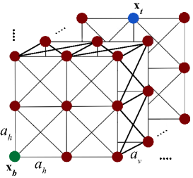
Figure 1: A fragment of the 3D path graph, arbitrary base position ${\bf x}_{b},$ and terminal position ${\bf x}_{t}$ .

IV Communication trajectory Optimization

Based on the acquired knowledge of the channel parameters from the learning phase, we are now concerned with the design of a communication trajectory in an uplink IoT data harvesting scenario. For the ease of exposition, the communication phase is designed based on the perfect channel model parameter estimates, while the impact of imperfect estimation is addressed in Section VI-B.

IV-A Communication System Model

We assume that the ground nodes are served by the drone in a time-division multiple access (TDMA) manner. Let $q_{k}[n]$ denotes the scheduling variable, then the TDMA constraints can be written as

$$\sum_{k=1}^{K}q_{k}[n]\leq 1\,,\,n\in[1,N_{c}],$$ (25)

$$q_{k}[n]\in\left\{0,1\right\},\,n\in[1,N_{c}],\,k\in[1,K],$$ (26)

where $q_{k}[n]=1$ indicates that the node $k$ is scheduled in time slot $n$. For the scheduled node, the average throughput is given by

$$C_{k}[n]=\text{E}\,\log_{2}\left(1+\frac{P\gamma_{k}[n]}{\sigma^{2}}\right),$$ (27)

where $\gamma_{k}[n]$ is the channel gain between the $k$-th node and the UAV at time step $n$, $P$ denotes the up-link transmission power of the ground node, and the additive white Gaussian noise power at the receiver is denoted by $\sigma^{2}$. Hence, the average achievable throughput of the $k$-th ground node over the course of the communication trajectory is given by

$$C_{k}=\frac{1}{N_{c}}\sum_{n=1}^{N_{c}}q_{k}[n]C_{k}[n].$$ (28)

IV-B Joint Scheduling and Trajectory Optimization

We consider the problem of efficient data harvesting where data originates from ground nodes and efficiency is meant in a max-min sense across the nodes. The problem of maximizing the minimum average throughput among all ground nodes by jointly optimizing node scheduling and UAV’s trajectory can be formulated as

$$\max_{\mathcal{X},z,Q}\ \underset{k\in[1,K]}{\min}\,C_{k}$$ (29a)

s.t. $$\left\|{\bf v}[n]-{\bf v}[n-1]\right\|\leq\rho_{max}\ ,n\in[2,N_{c}],$$ (29b)

$${\bf v}[1]={\bf v}[N_{c}],$$ (29c)

$$\eqref{eq:Alt_const},\,\eqref{eq:TDD_Cons},\,\eqref{eq:Sch_Var_Cons},$$ (29d)

where $Q=\{q_{k}[n],\,\forall n,\,\forall k\}$ is the set of scheduling variables, and $\mathcal{X}=\{(x[n],y[n]),\>\forall n\}$ denotes the discretized trajectory set of length $N_{c}$ in 2D. We assume that the drone flies at a fixed altitude $z[n]=z,\,\forall n$. The maximum speed constraint of the UAV is reflected in (29b), where $\rho_{max}=v_{max}T_{c}/N_{c}$. (29c) implies a possible loop trajectory constraint.

Problem (29) is challenging to solve due to the following issues:

• The scheduling variables $q_{k}[n]$ are binary and include integer constraints.

• The objective function (29a) is a non-convex with respect to the drone trajectory variables.

• Since the 3D city map, node locations, and UAV location at time $n$ are known, then in theory the LoS or NLoS status of the link can be finely predicted and, hence, the link gain $\gamma_{k}[n]$ can be computed from (2) up to the random shadowing. Unfortunately, such a direct exploitation of the rich raw map data leads to a highly non-differentiable problem in (29).

We overcome these difficulties by approximation using the same framework as [11] by employing the block-coordinate descent [22] and sequential convex programming [23] techniques. However, the key difference is that we optimize the drone’s altitude, and also exploit the 3D city map by introducing a statistical map compression approach that enables us to take into account the LoS and NLoS predictions.

IV-C LoS Probability Model Using Map Compression

Statistical map compression approach relies on converting 3D map data to build a reliable node location dependent LoS probability model. The LoS probability for the link between the drone located at altitude $z$ and the $k$-th ground node in the $n$-th time slot is given by

$$p_{k}[n]=\frac{1}{1+\exp(-a_{k}\theta_{k}[n]+b_{k})},$$ (30)

where $\theta_{k}[n]=\arctan(z/r_{k}[n])$ denotes the elevation angle and $r_{k}[n]$ is the ground projected distance between the drone and the $k$-th node located at ${\bf u}_{k}$ in the time slot $n$, and $\{a_{k},b_{k}\}$ are the model coefficients.

The LoS probability model coefficients $\{a_{k},b_{k}\}$ are learned (i.e. by utilizing logistic regression method[19]) by using a training data set formed by a set of tentative UAV locations around the $k$-th ground node along with the true LoS/NLoS label obtained from the 3D map. Interestingly, the model in (30) can be seen as a localized extension of the classical (global) LoS probability model used in [4, 5]. The key difference lies in the fact that, a local LoS probability model will give performance guarantees which a global model cannot.

Using (30), the average channel gain of the link between the drone and the $k$-th ground node in the $n$-th time slot is

$$\text{E}[\gamma_{k}[n]]= \left(\frac{d_{k}^{(A-1)\alpha_{\lx@glossaries@gls@link{acronym}{los}{\leavevmode\text{LoS}}}}-B}{1+\exp(-a_{k}\theta_{k}+b_{k})}+B\right)\frac{\beta_{\lx@glossaries@gls@link{acronym}{los}{\leavevmode\text{LoS}}}}{d_{k}^{\alpha_{\lx@glossaries@gls@link{acronym}{nlos}{\leavevmode\text{NLoS}}}}},$$ (31)

where $B=\frac{\beta_{\lx@glossaries@gls@link{acronym}{nlos}{\leavevmode\text{NLoS}}}}{\beta_{\lx@glossaries@gls@link{acronym}{los}{\leavevmode\text{LoS}}}},\,A=\frac{\alpha_{\lx@glossaries@gls@link{acronym}{nlos}{\leavevmode\text{NLoS}}}}{\alpha_{\lx@glossaries@gls@link{acronym}{los}{\leavevmode\text{LoS}}}}\geq 1$, and $d_{k}[n]=\sqrt{z^{2}+r_{k}^{2}[n]}$ is the distance between the $k$-th ground node and the drone. The details of the proof are given in Appendix -A.

V proposed solution for communication trajectory optimization

In this section, we first approximate the original optimization problem in (29) to a map-compressed problem and then present an iterative algorithm using block coordinate descent for solving it. Using (31) and the Jensen’s inequality, the average throughput upper-bound then can be written as

$$C_{k}^{\text{\text{up}}}=\frac{1}{N_{c}}\sum_{n=1}^{N_{c}}q_{k}[n]C_{k}^{\text{\text{up}}}[n]\ ,\,k\in[1,K],$$ (32)

where

$$C_{k}^{\text{\text{up}}}[n]=\log_{2}\left(1+\frac{P\,\text{E}[\gamma_{k}[n]]}{\sigma^{2}}\right).$$ (33)

We then approximate the original problem in (29) into the following map-compressed problem:

$$\max_{\mathcal{X},z,Q,\mu} \ \mu$$ (34a)

s.t. $$C_{k}^{\text{\text{up}}}\geq\mu\ ,\,\forall k,$$ (34b)

$$0\leq q_{k}[n]\leq 1\ ,\,\forall k,\,\forall n,$$ (34c)

$$\eqref{eq:GenProb_Dmax},\,\eqref{eq:GenProb_loopconst},\,\eqref{eq:Alt_const},\,\eqref{eq:TDD_Cons},$$ (34d)

where the constraints in (34c) represent the relaxation of the binary scheduling variable into continuous variables. Moreover, map compression allows us to circumvent the non-differentiability aspect of the original problem (29) by compressing the 3D map information into a probabilistic LoS model. However, (34) is still difficult to solve since it is a joint scheduling and path planning problem and is not convex. To make this problem more tractable, we split it up into three optimization sub-problems and then classically iterate between them to converge to a final solution. Note that, the iteration index of the proposed algorithm is denoted by “$j$”.

V-A Scheduling

For a given UAV planar trajectory $\mathcal{X}$ and altitude $z$, the ground node scheduling can be optimized as

$$\max_{Q,\mu}\ \ \mu$$ (35a)

s.t. $$\ C_{k}^{\text{\text{up}}}\geq\mu\ ,\,\forall k,$$ (35b)

$$\eqref{eq:TDD_Cons},\,\eqref{eq:Relaxed_Sche_Var}.$$

This problem is a standard Linear Program (LP) and can be solved by using any optimization tools such as CVX [24].

V-B Optimal Horizontal UAV Trajectory

For a given scheduling decision $Q$, and drone’s altitude $z$, we now aim to find the optimal planar trajectory by solving

$$\max_{\mathcal{X},\,\mu}\ \mu$$ (36a)

s.t. $$C_{k}^{\text{\text{up}}}\geq\mu\ ,\,\forall k,$$ (36b)

$$\eqref{eq:GenProb_Dmax},\,\eqref{eq:GenProb_loopconst}.$$ (36c)

The optimization problem (36) is not convex, since the constraint (36b) is neither convex nor concave. In general, there is no efficient method to obtain the optimal solution. Therefore, we adopt sequential convex programming technique for solving (36). To this end, the following results are helpful.

Lemma 1.

The function $h(x,y)\triangleq\text{$\log$}\left(1+f\left(x\right)g\left(y\right)\right)$ is convex if $\hat{h}(x,y)\triangleq\text{$\log$}\left(f\left(x\right)g\left(y\right)\right)$ is convex and $f(x)>0,\,\text{and }g(y)>0$.

Proof.

See Appendix -B. ∎

Proposition 1.

For any constant $\tau,\lambda>0$, the function $c(x,y,d)\triangleq\log\left(1+\left[(\frac{1}{1+x})(\frac{1}{y})+\tau\right]\frac{1}{d^{\lambda}}\right)$ is convex.

Proof.

See Appendix -C. ∎

By defining the auxiliary variables $f_{k}[n],\,w_{k}[n]$, $l_{k}[n]$, and $\theta_{k}[n]$, we can rewrite (36) as follows

$$\max_{\mathbb{V},\mathcal{X},\mu} \ \mu$$ (37a)

s.t. $$\frac{1}{N_{c}}\sum_{n=1}^{N_{c}}c_{k}^{\text{ }}\left(f_{k}[n],w_{k}[n],l_{k}[n]\right)\geq\mu\ ,\,\forall k,$$ (37b)

$$w_{k}[n]=\left(\left(z^{2}+l_{k}[n]\right)^{(A-1)\alpha_{\lx@glossaries@gls@link{acronym}{los}{\leavevmode\text{LoS}}}/2}-B\right)^{-1}\ ,\,\forall k,\,\forall n,$$ (37c)

$$f_{k}[n]=\exp\left(-a_{k}\theta_{k}[n]+b_{k}\right)\ ,\,\forall k,\,\forall n,$$ (37d)

$$l_{k}[n]=r_{k}^{2}[n]\ ,\,\forall k,\,\forall n,$$ (37e)

$$\theta_{k}[n]=\arctan\left(z/\sqrt{l_{k}[n]}\right)\ ,\,\forall k,\,\forall n,$$ (37f)

$$f_{k}[n],w_{k}[n],l_{k}[n],\theta_{k}[n]\geq 0\ ,\,\forall k,\,\forall n,$$ (37g)

$$\eqref{eq:GenProb_Dmax},\,\eqref{eq:GenProb_loopconst},$$ (37h)

where $\mathbb{V}=\{f_{k}[n],w_{k}[n],l_{k}[n],\theta_{k}[n]\,|\,\forall k,\,\forall n\}$ consists of all the auxiliary variables and

$$c_{k}^{\text{ }}\left(f_{k}[n],w_{k}[n],l_{k}[n]\right)\triangleq\qquad\qquad\qquad\qquad\qquad\qquad\qquad$$

$$\log_{2}\left(1+\left(\frac{1}{w_{k}[n](1+f_{k}[n])}+B\right)\frac{P\,\beta_{\lx@glossaries@gls@link{acronym}{los}{\leavevmode\text{LoS}}}}{\sigma^{2}\left(z^{2}+l_{k}[n]\right)^{\alpha_{\lx@glossaries@gls@link{acronym}{nlos}{\leavevmode\text{NLoS}}}/2}}\right).$$ (38)

Using Proposition 1, it can be easily seen that (38) is a convex function of variables $f_{k}[n],w_{k}[n],\text{ and }l_{k}[n]$. In constraint (37c), $w_{k}[n]$ can be convex or concave function depending on the value of $B$. However, in our case it is always convex since $z\geq h_{min}$, in a realistic scenario $\left(z^{2}+l_{k}[n]\right)^{(A-1)\alpha_{\lx@glossaries@gls@link{acronym}{los}{\leavevmode\text{LoS}}}/2}\gg B$. Moreover, all constraints (37d) to (37f) comprise convex functions. In order to solve problem (37), we utilize the sequential convex programming technique which solves instead the local linear approximation of the original problem. To form the local linear approximation, we use the given variables $\mathcal{X}^{j},z^{j}$ in the $j$-th iteration of the algorithm to convert the above problem to a standard convex form. For the ease of exposition, we use $c_{k}^{\text{ }}[n]$ instead of $c_{k}^{\text{ }}\left(f_{k}[n],w_{k}[n],l_{k}[n]\right)$. First, let’s start with constraint (37b), since any convex functions can be lower-bounded by its first order Taylor expansion, then we can write

$$\frac{1}{N_{c}}\sum_{n=1}^{N_{c}}q_{k}[n]c_{k}^{\text{ }}[n]\geq\frac{1}{N_{c}}\sum_{n=1}^{N_{c}}q_{k}[n]\tilde{c}_{k}^{\text{ }}[n]\geq\mu_{hp},$$

where $\tilde{c}_{k}^{\text{ }}[n]$ is an affine function and equals to the local first order Taylor expansion of $c_{k}^{\text{ }}[n]$ and $\mu_{hp}$ is a lower bound of $\mu$. Similarly, We can convert (37c) to (37f) into the standard convex form by replacing them with their first order Taylor expansion. We can approximate problem (37) as follows

$$\max_{\mathbb{V},\mathcal{X},\mu_{hp}} \ \mu_{hp}$$ (39a)

s.t. $$\frac{1}{N_{c}}\sum_{n=1}^{N_{c}}q_{k}[n]\tilde{c}_{k}^{\text{ }}[n]\geq\mu_{hp}\,,\,\forall k,$$ (39b)

$$f_{k}[n]\geq\widetilde{f}_{k}[n]\ ,\,\forall k,\,\forall n,$$ (39c)

$$w_{k}[n]\geq\widetilde{w}_{k}[n]\ ,\,\forall k,\,\forall n,$$ (39d)

$$l_{k}[n]\geq\widetilde{l}_{k}[n]\ ,\,\forall k,\,\forall n,$$ (39e)

$$\theta_{k}[n]\geq\widetilde{\theta}_{k}[n]\ ,\,\forall k,\,\forall n,$$ (39f)

$$\eqref{eq:EqualOptProb_Vge0},\,\eqref{eq:GenProb_Dmax},\,\eqref{eq:GenProb_loopconst},$$ (39g)

where the superscript “ ~ ” denotes the local first order Taylor expansion. Now, we have a standard convex problem which can be solved by any convex optimization tools like CVX. We denote the generated trajectory by solving (39) as $\mathcal{X}^{j+1}$.

V-C Optimal UAV Altitude

Now we proceed to optimize the UAV altitude for a given horizontal UAV trajectory $\mathcal{X}$ and scheduling decision $Q$. Similar to the preceding section, first we introduce auxiliary variables $h,\,m_{k}[n],\text{ and }o_{k}[n]$ consisting of convex functions as follows

$$m_{k}[n] =\exp\left(-a_{k}\arctan\left(z/r_{k}[n]\right)+b_{k}\right)\ ,\,\forall k,\,\forall n,$$

$$o_{k}[n] =\left(\left(h+r_{k}^{2}[n]\right)^{(A-1)\alpha_{\lx@glossaries@gls@link{acronym}{los}{\leavevmode\text{LoS}}}/2}-B\right)^{-1}\ ,\,\forall k,\,\forall n,$$

$$h =z^{2}.$$

In a similar manner to section V-B, we find the UAV altitude by using the sequential convex programming with given local point $z^{j}$ in the $j$-th iteration and the generated horizontal trajectory $\mathcal{X}^{j+1}$ in the last section. Finally, the UAV altitude is optimized as follows

$$\max_{\mathbb{W},z,\,\mu_{alt}}\ \mu_{alt}$$ (40a)

s.t. $$\frac{1}{N_{c}}\sum_{n=1}^{N_{c}}q_{k}[n]\,\tilde{c}_{k}[n]\geq\mu_{alt}\ ,\,\forall k,$$ (40b)

$$m_{k}[n]\geq\widetilde{m}_{k}[n]\ ,\,\forall k,\,\forall n,$$ (40c)

$$o_{k}[n]\geq\widetilde{o}_{k}[n]\ ,\,\forall k,\,\forall n,$$ (40d)

$$h\geq\widetilde{h},$$ (40e)

$$m_{k}[n],o_{k}[n],\,h>0,\,\forall k,\,\forall n,$$ (40f)

$$\eqref{eq:Alt_const},$$ (40g)

where $\tilde{c}_{k}[n]$ is the first order Taylor expansion of $c_{k}\left(m_{k}[n],o_{k}[n],h\right)$ which is a convex function and is defined similar to (38), and $\mathbb{W}=\left\{m_{k}[n],o_{k}[n],h\,|\,\forall k,\,\forall n\right\}$ comprises all the auxiliary variables. The superscript “ ~ ” denotes the local first order Taylor expansion, and $\mu_{alt}$ is a lower bound of $\mu$. We denote the drone altitude which is obtained by solving (40) as $z^{j+1}$ to be used in the next iteration.

V-D Iterative Algorithm

According to the preceding analysis, now we propose an iterative algorithm to solve the original optimization problem (29) by applying the block-coordinate descent method[22]. As mentioned earlier, we split up our problem into three phases (or blocks) of ground node scheduling, drone horizontal trajectory design, and flying altitude optimization over variables $\left\{Q,\mathcal{X},z\right\}$. In each iteration, we update just one set of variables at a time, rather than updating all the variables together, by fixing the other two sets of variables. Then, the output of each phase is used as an input for the next step. The rigorous description of this algorithm is summarized in Algorithm 1.

1. Initialize all variables $\left\{Q^{j},\mathcal{\mathcal{X}}^{j},z^{j}\right\}\,,j=1$.

2. Find the optimal solution of the scheduling problem (35) for given $\left\{\mathcal{\mathcal{X}}^{j},z^{j}\right\}$. Denote the optimal solution as $Q^{j+1}$.

3. Generate the optimal communication trajectory in horizontal plane ($\mathcal{\mathcal{X}}^{j+1}$) by solving (39) with given variables $\left\{Q^{j+1},\mathcal{\mathcal{X}}^{j},z^{j}\right\}$.

4. Solving optimization problem (40) given variables $\left\{Q^{j+1},\mathcal{\mathcal{X}}^{j+1},z^{j}\right\}$ and denote the solution as $z^{j+1}$.

5. Update $j:=j+1$.

6. Go to step 2 and repeat until the convergence (i.e. until observing a small increase in objective value).

Algorithm 1 Iterative algorithm for solving optimization problem (29).

V-E Proof of Convergence

In this section we prove the convergence of Algorithm 1 in a similar manner of [11]. To this end, in the $j$-th iteration we denote the $\mu(Q^{j},\mathcal{\mathcal{X}}^{j},z^{j}),\,\mu_{hp}(Q^{j},\mathcal{\mathcal{X}}^{j},z^{j}),\,\mu_{alt}(Q^{j},\mathcal{\mathcal{X}}^{j},z^{j})$ as the optimal objective values of problems (35), (39), and (40) , respectively. From step $(2)$ of Algorithm 1 for the given solution $Q^{j+1}$, we have

$$\mu(Q^{j},\mathcal{\mathcal{X}}^{j},z^{j})\leq\mu(Q^{j+1},\mathcal{\mathcal{X}}^{j},z^{j}),$$

since the optimal solution of problem (35) is obtained. Moreover, we can write

$$\mu(Q^{j+1},\mathcal{\mathcal{X}}^{j},z^{j}) \overset{(a)}{=}\mu_{hp}(Q^{j+1},\mathcal{\mathcal{X}}^{j},z^{j})$$

$$\overset{(b)}{\leq}\mu_{hp}(Q^{j+1},\mathcal{\mathcal{X}}^{j+1},z^{j})$$

$$\overset{(c)}{\leq}\mu(Q^{j+1},\mathcal{\mathcal{X}}^{j+1},z^{j}).$$

Step $(a)$ holds due to $\mu_{hp}(Q^{j+1},\mathcal{\mathcal{X}}^{j},z^{j})$ being a tight local first order Taylor approximation of problem (37) at the local points. Step $(b)$ is true, since we can find the optimal solution of problem (39) with the given variables $\{Q^{j+1},\mathcal{\mathcal{X}}^{j},z^{j}\}$, and $(c)$ holds because $\mu_{hp}(Q^{j+1},\mathcal{\mathcal{X}}^{j+1},z^{j})$ is the lower bound of the objective value $\mu(Q^{j+1},\mathcal{\mathcal{X}}^{j+1},z^{j})$. Then, by proceeding to step $(4)$ of Algorithm 1 and given variables $\{Q^{j+1},\mathcal{\mathcal{X}}^{j+1},z^{j}\}$, we obtain

$$\mu(Q^{j+1},\mathcal{\mathcal{X}}^{j+1},z^{j}) \overset{(d)}{=}\mu_{alt}(Q^{j+1},\mathcal{\mathcal{X}}^{j+1},z^{j})$$

$$\overset{(e)}{\leq}\mu_{alt}(Q^{j+1},\mathcal{\mathcal{X}}^{j+1},z^{j+1})$$

$$\overset{(f)}{\leq}\mu(Q^{j+1},\mathcal{\mathcal{X}}^{j+1},z^{j+1}).$$

Step $(d)$ is true since the local first order Taylor approximation in (40) is tight for the given local variables $\{Q^{j+1},\mathcal{\mathcal{X}}^{j+1},z^{j}\}$. $(e)$ holds since, the optimization problem (40) can be optimally solved, and $(f)$ is true due to $\mu_{alt}(Q^{j+1},\mathcal{\mathcal{X}}^{j+1},z^{j+1})$ is a lower bound of the objective value $\mu(Q^{j+1},\mathcal{\mathcal{X}}^{j+1},z^{j+1})$. Finally, we have

$$\mu(Q^{j},\mathcal{\mathcal{X}}^{j},z^{j})\leq\mu(Q^{j+1},\mathcal{\mathcal{X}}^{j+1},z^{j+1}).$$

Which indicates that the objective value of Algorithm 1 after each iteration is non-decreasing and since it is upper bounded by a finite value, so the convergence of Algorithm 1 is guaranteed.

V-F Trajectory Initializing

In this section, we propose a simple strategy to initialize the drone trajectory to be optimized later on by the introduced Algorithm 1. The initial trajectory is in form of a circle which is centered at ${\bf c}_{\text{trj}}=\left(x_{\text{trj}},y_{\text{trj}}\right)$ and the radius $r_{\text{trj}}$ which is given by

$$r_{\text{trj}}=\frac{L_{max}}{2\pi},$$

where $L_{max}=T_{c}\cdot v_{max}$. To determine the ${\bf c}_{\text{trj}}$, we use the notion of the (weighted) center of gravity of the ground nodes [7]. Moreover, the flying altitude is initialized at $h_{max}$.

VI Numerical Results

We consider a dense urban Manhattan-like area of size $600\times 600$ square meters, consisting of a regular street and buildings. The height of the building is Rayleigh distributed within the range of $5$ to $40$ meters [4]. The average building height is $14$ m. True propagation parameters are chosen as $\alpha_{\lx@glossaries@gls@link{acronym}{los}{\leavevmode\text{LoS}}}=2.27,\,\alpha_{\lx@glossaries@gls@link{acronym}{nlos}{\leavevmode\text{NLoS}}}=3.64,\,\ss_{\lx@glossaries@gls@link{acronym}{los}{\leavevmode\text{LoS}}}=-30\,\text{dB},\,\ss_{\lx@glossaries@gls@link{acronym}{nlos}{\leavevmode\text{NLoS}}}=-40\,\text{dB}$ according to an urban micro scenario in [20]. The variances of the shadowing component in LoS and NLoS scenarios are $\sigma_{\lx@glossaries@gls@link{acronym}{los}{\leavevmode\text{LoS}}}^{2}=2$ and $\sigma_{\lx@glossaries@gls@link{acronym}{nlos}{\leavevmode\text{NLoS}}}^{2}=5$, respectively. The transmission power for ground nodes is chosen as $P=30$ dBm, and the noise power at the receiver is -80 dBm. The UAV has a maximum speed of $v_{max}=10\,\text{m}/\text{s}$.

VI-A Learning Trajectory

(a)
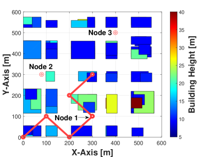
(b)

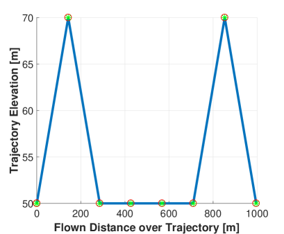
Figure 2: (a) Top view of the optimal learning trajectory using proposed algorithm. (b) The UAV elevation along the trajectory.

An illustration of the optimal learning trajectory is presented in Fig. 2 for $K=3$ ground nodes. In this scenario, the UAV flies from the base position ${\bf x}_{b}(0,0,50)$ towards the terminal location ${\bf x}_{t}=(300,300,50)$ under the flight time constraint $T_{l}=100\,\text{s}$. To discretize the search space over the city for creating the 3D path graph, we chose $a_{h}=100$ m and $a_{v}=20$ m as defined in section III-C. It is interesting to note that, the trajectory experiences a wide array of altitudes there by improving the learning performance of both LoS and NLoS segments. For the ease of exhibition, we plotted the generated trajectory in two different figures. Fig. 2-a shows the top view of the generated trajectory while the elevation of the trajectory as a function of the flown distance is depicted in Fig. 2-b.

In Fig. 3 the performance of the optimal trajectory in terms of the mean squared error (MSE) of the learned channel parameters $(\alpha_{s},\ss_{s};s=\left\{\lx@glossaries@gls@link{acronym}{los}{\leavevmode\text{LoS}},\lx@glossaries@gls@link{acronym}{nlos}{\leavevmode\text{NLoS}}\right\})$ is shown as a function of the number of ground nodes. The duration of the learning phase $T_{l}=100$ s. We perform Monte-Carlo simulations over random user locations. We also compare the performance of the optimal trajectory with that of randomly generated arbitrary trajectories. For a given realization, arbitrary trajectory of duration $T_{l}$ is generated. It is clear that, the channel can be learned more precisely by taking the optimized learning trajectory. Also, the learning error is reduced when the number of ground nodes increases, since the chance of obtaining measurement from both LoS and NLoS segments increases.

VI-B Communication Trajectory

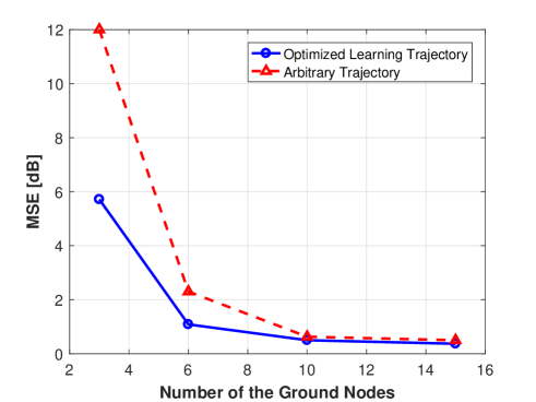
Figure 3: Comparison of the MSE for different learning trajectories.

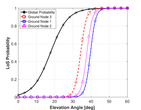
Figure 4: Global LoS probability compared with the local LoS probability learned form the 3D map for three ground nodes.

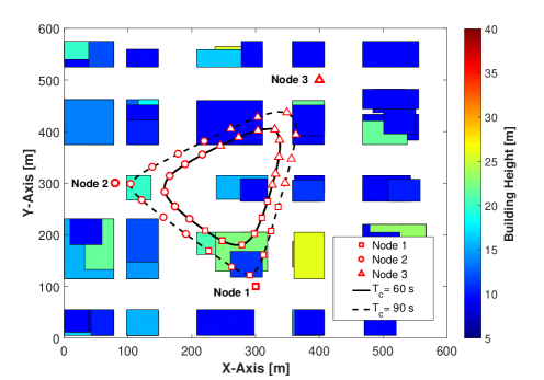
Figure 5: Optimal drone trajectory and ground node scheduling for different flight times. As the flight time increases, the UAV gets closer to individual ground nodes.

In this section, we evaluate the performance of the communication path planning algorithm. Since the communication trajectory design depends on the local LoS probability model, we first need to learn the probability model coefficients in (30). For this, we employed the logistic regression method on the training data set obtained by randomly sampling around each ground node. The labeling is done with the true LoS status obtained from the 3D city map. Fig.4 shows the obtained LoS probabilities for $K=3$ ground nodes whose locations are shown in Fig. 5. We also plot the global LoS probability which is computed from the characteristics of the 3D map according to [4]. It is clear that the local probabilities have the sharper transitions and thus provide more information per ground node (i.e. if the node is surrounded by the tall buildings or is in a large open area), while the global probability can be considered as the average of the local LoS probability of the nodes in different locations.

In Fig. 5, we show the generated trajectory over the city buildings for different flight times $(T_{c})$. It is clear that by increasing $T_{c}$, the UAV exploits the flight time to improve the ground node link quality by enlarging the trajectory and moving towards the ground nodes. It is crucial to note that the generated trajectory is closer to the ground nodes which has the less LoS probability (i.e. the ground nodes who are close to buildings or surrounded by tall skyscrapers). In Fig. 5, the drone tries to get closer to the ground nodes 1 and 2 since they are close to the buildings which mostly block the LoS link to the drone. Moreover, we illustrated the result of the ground node scheduling during the trajectory with different markers which are assigned to each node. Namely triangles, squares, and circles pertain, respectively, to ground nodes 1 to 3. For example, square markers shown on the trajectory indicate that the drone is serving the ground node 1 at that time.

We then outline the convergence behavior of Algorithm 1 by assuming $K=3$ and $T_{c}=90$ s. The drone altitude and worst ground node throughput versus iteration are shown in Fig.6. As we expected, the worst ground node throughput in each iteration improves and finally converges to a finite value.

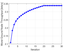
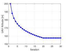
(a)	(b)

Figure 6: (a) Throughput performance versus iteration and (b) drone altitude evolution versus iteration.

In Fig. 7, the performance of the proposed map-based algorithm in comparison with two other approaches, which are briefly explained below, versus the flight time by considering $K=6$ ground nodes is shown.

• Probabilistic algorithm

  In the probabilistic approach, we consider the same trajectory design algorithm as proposed in this paper with the difference that for a link between the drone located at altitude $z$ and the $k$-th ground node, the LoS probability at the time step $n$ is given by

  $$p_{k}[n]=\frac{1}{1+\exp\left(-a\,\theta_{k}[n]+b\right)},$$

  where parameters $\left\{a,b\right\}$ are computed according to [4] and based on the characteristics of the 3D map. In other words, we use a global LoS probability model.

• Deterministic algorithm

  In the deterministic algorithm, an optimal trajectory is generated based on the method introduced in [11] which considers a single deterministic LoS channel model for the link between the drone and the ground nodes. In order to have a fair comparison, we modified this method by using an average path-loss instead of the pure LoS channel model. the channel parameters pertaining to the average path-loss model are learned by fitting one channel model for the whole measurements gathered from both LoS and NLoS ground nodes.

We have also investigated the impact of the imperfect estimation of the channel parameters on the performance of the map-based algorithm. The result of the algorithm using the learned channel parameters is illustrated in Fig. 7. As it can be seen, the channel estimation uncertainty stemming from the learning part has a minor effect on the performance of the map-based algorithm and in general the map-based algorithm outperforms the other approaches which is expected since in the proposed algorithm we utilize more information through the 3D map.

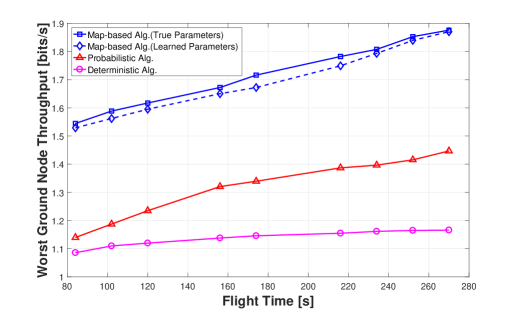
Figure 7: Performance of the map-based algorithm for the learned and true channel parameters in comparison with the probabilistic approach and the deterministic Algorithm for 6 ground nodes versus increasing the flight time.

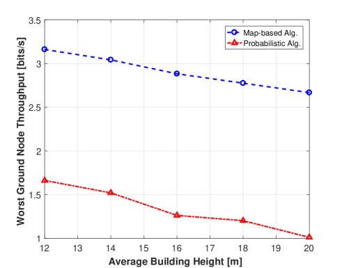
Figure 8: Performance comparison of the map-based Algorithm and the probabilistic approach versus the average building height for a fixed flight time.

In Fig. 8 a performance comparison of the proposed map-based algorithm and the probabilistic approach under a fixed flight time by increasing the average buildings height is illustrated. The map-based algorithm provides a better services to the ground nodes. For both algorithms by increasing the buildings height, the performance degraded since it is more likely that the link between the ground nodes and the drone over the course of the trajectory being NLoS.

VII Conclusion

This work has considered the problem of trajectory design for an UAV BS that is providing communication services for a number of ground nodes in the context of an IoT data harvesting scenario. In contrast to the existing literature, we assume that the propagation parameters are unknown and we devise an optimized trajectory for the UAV that allows it to learn the parameters efficiently. The learning trajectory optimization relies on the dynamic programming techniques and the knowledge of the 3D city map. Once the channel parameters are learned, we have developed throughput-optimized trajectories such that the amount of data collected from each of the ground nodes is maximized. We have proposed an iterative algorithm that leverages the knowledge of the 3D city map via a novel map-compression method and uses the block coordinate descent and sequential convex programming techniques. It is also shown that the proposed algorithm is guaranteed to converge to at least a locally optimal solution. The advantages of the learning trajectory optimization and communication path planning algorithm by utilizing the proposed map compression method are illustrated in an urban IoT setting.

-A Proof of the average channel gain

The average channel gain of the link between the drone and the $k$-th ground node in the $n$-th time slot is given by

$$\text{E}[\gamma_{k}[n]] =p_{k}[n]\gamma_{\lx@glossaries@gls@link{acronym}{los}{\leavevmode\text{LoS}},k}[n]+(1-p_{k}[n])\gamma_{\lx@glossaries@gls@link{acronym}{nlos}{\leavevmode\text{NLoS}},k}[n],$$ (41)

where $p_{s,k}[n]$ denotes the LoS probability, $\gamma_{\lx@glossaries@gls@link{acronym}{los}{\leavevmode\text{LoS}},k}[n]$ and $\gamma_{\lx@glossaries@gls@link{acronym}{nlos}{\leavevmode\text{NLoS}},k}[n]$, respectively, denote the channel gain in LoS and NLoS propagation segments. Expanding (41) we have

$$\text{E}[\gamma_{k}[n]]\overset{(a)}{=}\, p_{k}[n]\frac{\beta_{\lx@glossaries@gls@link{acronym}{los}{\leavevmode\text{LoS}}}}{d_{k}^{\alpha_{\lx@glossaries@gls@link{acronym}{los}{\leavevmode\text{LoS}}}}[n]}+(1-p_{k}[n])\frac{\beta_{\lx@glossaries@gls@link{acronym}{nlos}{\leavevmode\text{NLoS}}}}{d_{k}^{\alpha_{\lx@glossaries@gls@link{acronym}{nlos}{\leavevmode\text{NLoS}}}}[n]}$$

$$\overset{(b)}{=} \left(\frac{d_{k}^{(A-1)\alpha_{\lx@glossaries@gls@link{acronym}{los}{\leavevmode\text{LoS}}}}-B}{1+\exp\left(-a_{k}\theta_{k}+b_{k}\right)}+B\right)\frac{\beta_{\lx@glossaries@gls@link{acronym}{los}{\leavevmode\text{LoS}}}}{d_{k}^{\alpha_{\lx@glossaries@gls@link{acronym}{nlos}{\leavevmode\text{NLoS}}}}},$$ (42)

where step $(a)$ holds by substituting the values of $\gamma_{\lx@glossaries@gls@link{acronym}{los}{\leavevmode\text{LoS}},k}[n]$ and $\gamma_{\lx@glossaries@gls@link{acronym}{nlos}{\leavevmode\text{NLoS}},k}[n]$ form (2) into (41), $(b)$ is obtained by substituing (30), where $B=\frac{\beta_{\lx@glossaries@gls@link{acronym}{nlos}{\leavevmode\text{NLoS}}}}{\beta_{\lx@glossaries@gls@link{acronym}{los}{\leavevmode\text{LoS}}}},\,A=\frac{\alpha_{\lx@glossaries@gls@link{acronym}{nlos}{\leavevmode\text{NLoS}}}}{\alpha_{\lx@glossaries@gls@link{acronym}{los}{\leavevmode\text{LoS}}}}\geq 1$, and $d_{k}[n]=\sqrt{z^{2}+r_{k}^{2}[n]}$ is the distance between the $k$-th ground node and the drone. Note that, in order to ease the notation, the average random shadowing is assumed absorbed into $\beta_{s}$ in (42) i.e., $\beta_{s}\triangleq\beta_{s}exp(\sigma_{s}^{2}/2)$ , $s\in\{\lx@glossaries@gls@link{acronym}{los}{\leavevmode\text{LoS}},\lx@glossaries@gls@link{acronym}{nlos}{\leavevmode\text{NLoS}}\}$.

-B Proof of Lemma 1

By proving that the Hessian of the function $h\triangleq h(x,y)$, is a positive semi-definite (PSD) matrix, we prove the convexity of $h$. We start by considering the Hessian of function $\hat{h}\triangleq\hat{h}(x,y)$

$$\nabla^{2}\hat{h}=\left[\begin{array}[]{cc}\frac{f_{xx}f-f_{x}^{2}}{f^{2}}&0\\ 0&\frac{g_{yy}g-g_{y}^{2}}{g^{2}}\end{array}\right]\geq 0,$$ (43)

where $f\triangleq f(x)$, $g\triangleq g(x)$, $f_{x}\triangleq\frac{\partial f}{\partial x}$, $g_{y}\triangleq\frac{\partial g}{\partial y}$, $f_{xx}\triangleq\frac{\partial^{2}f}{\partial x^{2}}$, and $g_{yy}\triangleq\frac{\partial^{2}g}{\partial y^{2}}$. Since $\hat{h}$ is convex, $\nabla^{2}\hat{h}$ is PSD and has non-negative diagonal elements. Hence, for $f>0$, $g>0$,

$$f_{xx}\geq\frac{f_{x}^{2}}{f} ,g_{yy}\geq\frac{g_{y}^{2}}{g}.$$ (44)

Also, it can easily be deduced that

$$f_{xx}g\geq 0,\,g_{yy}f\geq 0.$$ (45)

The hessian of $h\triangleq h(x,y)$ is given by

$$\nabla^{2}h=\left[\begin{array}[]{cc}\frac{g^{2}\left(f_{xx}f-f_{x}^{2}\right)+f_{xx}g}{\left(1+fg\right)^{2}}&\frac{f_{x}g_{y}}{\left(1+fg\right)^{2}}\\ \frac{f_{x}g_{y}}{\left(1+fg\right)^{2}}&\frac{f^{2}\left(g_{yy}g-g_{y}^{2}\right)+g_{yy}f}{\left(1+fg\right)^{2}}\end{array}\right].$$

If $\det(\nabla^{2}h)\geq 0$ and $\text{tr}(\nabla^{2}h)\geq 0$, then $\nabla^{2}h$ is PSD [25]. Let us rewrite $\nabla^{2}h$ as a summation of two matrices $\nabla^{2}h={\bf M}_{1}+{\bf M}_{2}$, where

$${\bf M}_{1} =\left[\begin{array}[]{cc}\frac{g^{2}\left(f_{xx}f-f_{x}^{2}\right)}{\left(1+fg\right)^{2}}&0\\ 0&\frac{f^{2}\left(g_{yy}g-g_{y}^{2}\right)}{\left(1+fg\right)^{2}}\end{array}\right],$$

$${\bf M}_{2} =\left[\begin{array}[]{cc}\frac{f_{xx}g}{\left(1+fg\right)^{2}}&\frac{f_{x}g_{y}}{\left(1+fg\right)^{2}}\\ \frac{f_{x}g_{y}}{\left(1+fg\right)^{2}}&\frac{g_{yy}f}{\left(1+fg\right)^{2}}\end{array}\right].$$

Since $\det(\nabla^{2}h)$ is a $2\times 2$ matrix, we can write it as [26],

$$\det(\nabla^{2}h)=\det({\bf M}_{1})+\det({\bf M}_{2})+\text{tr}({\bf M}_{1}^{\dagger}{\bf M}_{2}),$$

where ${\bf M}_{1}^{\dagger}$ is the adjugate of ${\bf M}_{1}$. From (43), it can easily be shown that $\det({\bf M}_{1})\geq 0$. Also, using (44) we can see that

$$\det({\bf M}_{2}) =\left(1+fg\right)^{-2}\left[(f_{xx}f)\,(g_{yy}g)-f_{x}^{2}g_{y}^{2}\right]$$

$$\geq 0.$$

Finally, from (43) and (45), we have

$$\text{tr}({\bf M}_{1}^{\dagger}{\bf M}_{2}) =f^{2}\left(g_{yy}g-g_{y}^{2}\right)f_{xx}g+g^{2}\left(f_{xx}f-f_{x}^{2}\right)g_{yy}f$$

$$\geq 0.$$

Therefore, we can conclude that $\det(\nabla^{2}h)\geq 0$. It remains to prove that $\text{tr}\left(\nabla^{2}h\right)\geq 0$. Using (43) and (45), we can see that the diagonal elements of $\nabla^{2}h$ are positive and hence the $\text{tr}\left(\nabla^{2}h\right)\geq 0$. Consequently, we can see $\nabla^{2}h$ is PSD, which concludes the proof.

-C Proof of Proposition 1

Let $f(x)=\frac{1}{1+x}$, $g(y)=\frac{1}{y}$, $h(d)=1/d^{\lambda}$ and $q(x,y)=f(x)g(y)+\tau,\,\tau\geq 0$. For positive $f\triangleq f(x)$ and $g\triangleq g(y)$, since $\log(f\,g)$ is strictly convex, using Lemma 1, we can infer that $\log\left(q(x,y)\right)$ is also strictly convex. Finally, from the above arguments we can easily see that the function

$$\hat{c}(x,y,d)=\log\left(q(x,y)\,h(d)\right),\,k\geq 0$$

is also strictly convex.

The Hessian of $\hat{c}(x,y,d)$ is given by

$$\nabla^{2}\hat{c}=\left[\begin{array}[]{ccc}\frac{\left(q_{xx}q-q_{x}^{2}\right)}{q^{2}}&\frac{\left(q_{xy}q-q_{x}q_{y}\right)}{q^{2}}&0\\ \frac{\left(q_{yx}q-q_{x}q_{y}\right)}{q^{2}}&\frac{\left(q_{yy}q-q_{y}^{2}\right)}{q^{2}}&0\\ 0&0&\frac{\left(h_{dd}h-h_{d}^{2}\right)}{h^{2}}\end{array}\right],$$ (46)

where $q\triangleq q(x,y)$ and $h\triangleq h(d)$. $q_{x},\,q_{xy}$ stand for the partial derivative of $q$ and are defined as $q_{x}=\frac{\partial q}{\partial x},\,q_{yx}=q_{xy}=\frac{\partial^{2}q}{\partial x\partial y}$. $q_{xx},q_{yy},h_{d},h_{dd}$ also are defined similarly. Since $\nabla^{2}\hat{c}$ is a positive definite (PD) and symmetric matrix, it has positive diagonal elements. Hence,

$$q_{xx}>\frac{q_{x}^{2}}{q}>0.$$ (47)

Since $h>0$, from (47) we have

$$h\,q_{xx}>0.$$ (48)

Moreover, since $\log\left(f\,g\right)$ is strictly convex, we can write

$$f_{xx}f>f_{x}^{2},\ g_{yy}g >g_{y}^{2}.$$ (49)

Using the above results, we now prove that the function

$$c(x,y,d)=\log\left(1+q(x,y)\,h(d)\right)$$

is convex. The Hessian of $c\triangleq c(x,y,d)$ is

$$\nabla^{2}c=\frac{1}{\left(1+q\,h\right)^{2}}\left({\bf P}+{\bf Q}\right),$$

where

$${\bf P}= \left(q\,h\right)^{2}\nabla^{2}\hat{c},$$

$${\bf Q}= \left[\begin{array}[]{ccc}q_{xx}h&q_{xy}h&q_{x}h_{d}\\ q_{yx}h&q_{yy}h&q_{y}h_{d}\\ q_{x}h_{d}&q_{y}h_{d}&q\,h_{dd}\end{array}\right].$$

Matrix ${\bf P}$ is PD since $\nabla^{2}\hat{c}$ is PD and $q,h>0$. In order to show that the Hessian matrix $\nabla^{2}c$ is PD, we need to prove that ${\bf Q}$ is PD as the sum of two PD matrices is PD. According to [27], if all upper left $n\times n$ determinants of a symmetric matrix are positive, the matrix is PD. Matrix ${\bf Q}$ is symmetric, since $q_{xy}$ and $q_{yx}$ are equal to $f_{x}\,g_{y}$.

We start from the upper left $1\times 1$ determinants of ${\bf Q}$ which equals to $q_{xx}h$. It follows from (48), that $q_{xx}h>0$. Now, we proceed to show that the determinant of upper left $2\times 2$ matrix of ${\bf Q}$ is positive. So, we can write

$$\frac{\det\left({\bf Q}_{2\times 2}\right)}{h^{2}} =\left(q_{xx}\,q_{yy}-q_{xy}^{2}\right)$$ (50)

$$\overset{\left(a\right)}{=}(f_{xx}f)(g_{xx}g)-f_{x}^{2}g_{y}^{2}$$ (51)

$$\overset{\left(b\right)}{>}0,$$ (52)

where ${\bf Q}_{2\times 2}$ denotes the upper left $2\times 2$ matrix of ${\bf Q}$, $(a)$ is obtained by substituting $q_{xx}=f_{xx}g,\,q_{yy}=g_{yy}f,\>q_{xy}=f_{x}\,g_{y}$ in (50) and step $(b)$ follows from (49). Then, we compute

$$\det\left({\bf Q}\right) =h_{d}^{2}\left(h\,m\right)+h_{dd}h\left(h\,q\,p\right),$$

where $m=2q_{xy}q_{x}q_{y}-q_{xx}q_{y}^{2}-q_{yy}q_{x}^{2},\,p=q_{xx}q_{yy}-q_{xy}^{2}$. From (49), it can be shown that $m<0$. From the convexity of $\hat{c}(x,y,d)$ , by computing the determinant of upper left $2\times 2$ matrix of $\nabla^{2}\hat{c}$ and performing some algebraic reductions we obtain

$$m+q\,p>0$$

$$\Rightarrow h\,q\,p>-h\,m>0.$$ (53)

Also, since $\log\left(h\right)$ is strictly convex, we can write

$$h_{dd}h>h_{d}^{2}.$$ (54)

Therefore, according to (53), (54), it can be seen that $\det\left({\bf Q}\right)>0$. Since all upper left $n\times n$ determinants of ${\bf Q}$ are positive, we conclude that the matrix ${\bf Q}$ is PD. Hence, $\nabla^{2}c$ is also PD.

Omid Esrafilian received the B.Sc. degree in control and electrical engineering from K. N. Toosi University of Technology, Tehran, Iran, in 2014. He was accepted as a talented student for M.Sc. studies and he graduated as the ranked first student from K. N. Toosi University of Technology, Tehran, Iran, in 2016. He is currently pursuing the Ph.D. degree at EURECOM (Sorbonne University). He received awards from robotic competitions in the level of national and international. His main research interests include unmanned aerial vehicle communication, path planning and optimization, robotics, and control theory.

Rajeev Gangula (S’13, M’15) received the M.Tech. degree specializing in signal processing from Indian Institute of Technology, Guwahati, in June 2010. He obtained the M.Sc. and Ph.D. degrees from Telecom ParisTech (EURECOM) in 2011 and 2015, respectively. He was awarded the Orange-MEEA scholarship for M.Sc. studies. His research interests lie in the areas of optimization and communication theory.

David Gesbert (IEEE Fellow) is Professor and Head of the Communication Systems Department, EURECOM. He obtained the Ph.D. degree from Ecole Nationale Superieure des Telecommunications, France, in 1997. From 1997 to 1999 he has been with the Information Systems Laboratory, Stanford University. He was then a founding engineer of Iospan Wireless Inc, a Stanford spin off pioneering MIMO-OFDM (now Intel). Before joining EURECOM in 2004, he has been with the Department of Informatics, University of Oslo as an adjunct professor. D. Gesbert has published about 280 papers and 25 patents, some of them winning the 2015 IEEE Best Tutorial Paper Award (Communications Society), 2012 SPS Signal Processing Magazine Best Paper Award, 2004 IEEE Best Tutorial Paper Award (Communications Society), 2005 Young Author Best Paper Award for Signal Proc. Society journals, and paper awards at conferences 2011 IEEE SPAWC, 2004 ACM MSWiM. He has been a Technical Program Co-chair for ICC2017. He was named a Thomson-Reuters Highly Cited Researchers in Computer Science. Since 2015, he holds the ERC Advanced grant “PERFUME”on the topic of smart device Communications in future wireless networks. He held visiting professor positions in KTH (2014) and TU Munich (2016). Since 2017 he is also a visiting Academic Master within the Program 111 at the Beijing University of Posts and Telecommunications. He sits in a Board of Directors for the OpenAirInterface Software Alliance.

References

- [1] Y. Zeng, R. Zhang, and T. J. Lim, “Wireless communications with unmanned aerial vehicles: opportunities and challenges,” IEEE Communications Magazine, vol. 54, no. 5, pp. 36–42, 2016.
- [2] S. Hayat, E. Yanmaz, and R. Muzaffar, “Survey on unmanned aerial vehicle networks for civil applications: A communications viewpoint,” IEEE Communications Surveys & Tutorials, vol. 18, no. 4, pp. 2624–2661, 2016.
- [3] M. Mozaffari, W. Saad, M. Bennis, Y.-H. Nam, and M. Debbah, “A tutorial on UAVs for wireless networks: Applications, challenges, and open problems,” arXiv preprint arXiv:1803.00680, 2018.
- [4] A. Al-Hourani, S. Kandeepan, and S. Lardner, “Optimal LAP altitude for maximum coverage,” IEEE Wireless Communications Letters, vol. 3, no. 6, pp. 569–572, 2014.
- [5] M. Mozaffari, W. Saad, M. Bennis, and M. Debbah, “Optimal transport theory for power-efficient deployment of unmanned aerial vehicles,” in IEEE International Conference on Communications (ICC), 2016.
- [6] M. Alzenad, A. El-Keyi, F. Lagum, and H. Yanikomeroglu, “3-D placement of an unmanned aerial vehicle base station (UAV-BS) for energy-efficient maximal coverage,” IEEE Wireless Communications Letters, vol. 6, no. 4, pp. 434–437, 2017.
- [7] O. Esrafilian and D. Gesbert, “Simultaneous User Association and Placement in Multi-UAV Enabled Wireless Networks,” in 22nd International ITG Workshop on Smart Antennas (WSA). VDE, 2018.
- [8] Ladosz Pawel and Hyondong Oh and Wen-Hua Chen, “Optimal positioning of communication relay unmanned aerial vehicles in urban environments.” in IEEE International Conference on Unmanned Aircraft Systems (ICUAS), 2016.
- [9] J. Chen and D. Gesbert, “Optimal positioning of flying relays for wireless networks: A LOS map approach,” in IEEE International Conference on Communications (ICC), 2017.
- [10] R. Gangula, P. de Kerret, O. Esrafilian, and D. Gesbert, “Trajectory optimization for mobile access point,” in IEEE 51st Asilomar Conference on Signals, Systems, and Computers, 2017.
- [11] Wu, Qingqing, Y. Zeng, and R. Zhang, “Joint trajectory and communication design for multi-UAV enabled wireless networks.” IEEE Transactions on Wireless Communications, vol. 17, no. 3, pp. 2109–2121, 2018.
- [12] A. T. Klesh, P. T. Kabamba, and A. R. Girard, “Path planning for cooperative time-optimal information collection,” in IEEE American Control Conference, 2008.
- [13] Y. Zeng, R. Zhang, and T. J. Lim, “Throughput maximization for UAV-enabled mobile relaying systems,” IEEE Transactions on Communications, vol. 64, no. 12, pp. 4983–4996, 2016.
- [14] Y. Zeng and R. Zhang, “Energy-efficient UAV communication with trajectory optimization,” IEEE Trans. Wireless Commun, vol. 16, no. 6, pp. 3747–3760, 2017.
- [15] A. Goldsmith, Wireless communications. Cambridge university press, 2005.
- [16] J. Chen, U. Yatnalli, and D. Gesbert, “Learning radio maps for UAV-aided wireless networks: A segmented regression approach,” in IEEE International Conference on Communications (ICC), 2017.
- [17] J. Chen, O. Esrafilian, D. Gesbert, and U. Mitra, “Efficient algorithms for air-to-ground channel reconstruction in UAV-aided communications,” in IEEE Globecom Workshop on Wireless Networking and Control for Unmanned Autonomous Vehicles, 2017.
- [18] O. Esrafilian and D. Gesbert, “3D city map reconstruction from UAV-based radio measurements,” in IEEE Global Communication Conference (GLOBECOM), 2017.
- [19] S. Rogers and M. Girolami, A first course in machine learning. CRC Press, 2016.
- [20] 3GPP TR 38.901 version 14.0.0 Release 14, “Study on channel model for frequencies from 0.5 to 100 GHz,” ETSI, Tech. Rep., 2017.
- [21] D. E. Kirk, Optimal control theory: an introduction. Courier Corporation, 2012.
- [22] Y. Xu and W. Yin, “A block coordinate descent method for regularized multiconvex optimization with applications to nonnegative tensor factorization and completion.” SIAM Journal on imaging sciences, vol. 6, no. 3, pp. 1758–1789, 2013.
- [23] Q. T. Dinh and M. Diehl, “Local convergence of sequential convex programming for nonconvex optimization.” Recent Advances in Optimization and its Applications in Engineering, pp. 93–102, 2010.
- [24] M. Grant, S. Boyd, and Y. Ye, “CVX: Matlab software for disciplined convex programming, version 2.0 beta. http://cvxr.com/cvx.” 2013.
- [25] E. D. Klerk, Appendix A of Aspects of semidefinite programming: interior point algorithms and selected applications. Springer Science & Business Media, 2006, vol. 65.
- [26] U. Prells, M. I. Friswell, and S. D. Garvey, “Use of geometric algebra: compound matrices and the determinant of the sum of two matrices.” in Proceedings of the Royal Society of London A: Mathematical, Physical and Engineering Sciences, vol. 459, no. 2030. The Royal Society, 2003, pp. 273–285.
- [27] G. Strang, Section 6.5 of Introduction to linear algebra. Wellesley, MA: Wellesley-Cambridge Press, 1993, vol. 3.