The entrainment matrix of a superfluid nucleon mixture at finite temperatures

Abstract

It is considered a closed system of non-linear equations for the entrainment matrix of a non-relativistic mixture of superfluid nucleons at arbitrary temperatures below the onset of neutron superfluidity, which takes into account the essential dependence of the superfluid energy gap in the nucleon spectra on the velocities of superfluid flows. It is assumed that the protons condense into the isotropic ¹S₀ state, and the neutrons are paired into the spin-triplet ³P₂ state. It is derived an analytic solution to the non-linear equations for the entrainment matrix under temperatures just below the critical value for the neutron superfluidity onset. In general case of an arbitrary temperature of the superfluid mixture the non-linear equations are solved numerically and fitted by simple formulas convenient for a practical use with an arbitrary set of the Landau parameters.

1 Introduction

It is usually assumed that neutron stars (NSs) are composed mainly of superfluid nucleons (see, e.g. Takatsuka, 1972; Shternin et al., 2011). After the pioneering work by Tamagaki (1970), it is adopted to assume that the superfluid protons are paired into the spin singlet ¹S₀, and the superfluid neutrons are in the spin-triplet ³P₂ state in the NS core. Observations of pulsating NSs, which make it possible to obtain a unique information on the properties of the superdense matter, are of a great interest (see, e.g. Andersson et al., 1999; Andersson, 1998; Friedman & Morsink, 1998; Andersson et al., 2003; Andersson & Kokkotas, 2001; Gusakov et al., 2014; Arras et al., 2003; Gusakov et al., 2005; Sidery et al., 2010; Prix & Rieutord, 2002). The hydrodynamic theory describing global pulsations of superfluid NSs must necessarily involve the non-dissipative coupling between the nucleons in the NS interior known as the entrainment effect. Another phenomenon that is also influenced by the entrainment is the post-glitch response of the NSs. The core of the star, consisting of the neutron superfluid and plasma of electrons, muons, superconducting protons and, probably, charged and neutral hyperons responds to the glitch via magnetic, viscous and mutual friction forces (Alpar et al., 1984). The mutual entrainment in the superfluid nucleon mixture directly influences the star’s response following a glitch via the strong impact on kinetic coefficients of the NS matter, in particular, on the bulk and shear viscosities (Alford et al., 2012; Haensel et al., 2000, 2001; Shternin & Yakovlev, 2008).

The entrainment effect was included in the rotational dynamics of pulsars and in the hydrodynamics of NS pulsations by many authors within the framework of the Fermi liquid theory (see, e.g. Prix & Rieutord, 2002; Prix et al., 2002; Prix, 2004; Gusakov & Andersson, 2006; Chugunov & Gusakov, 2011). Usually the mutual entrainment of supercurrents is described with the aid of the entrainment matrix first introduced by Andreev and Bashkin (Andreev & Bashkin, 1975) in the hydrodynamics of the superfluid mixture ³He and ⁴He. For the baryon matter of a NS core the most interest represents the entrainment matrix which relates the mass current density of the baryons with the relative velocity of their superfluid and normal components.

For the case of zero temperature the entrainment matrix of the superfluid neutron-proton mixture was calculated in Borumand et al. (1996); Comer & Joynt (2003); Chamel & Haensel (2006); Gusakov et al. (2009a). These calculations assume that the energy gaps of superfluid nucleons are constant and, because of a strong dependence of the energy gaps on superfluid velocities, are valid only for small amplitudes of the neutron star’s pulsations. Namely, the superfluid velocities of the neutron and proton flows relative the normal (non-superfluid) nucleons should be small as compared to the critical flow velocity at which the superfluidity is destroyed. The formalism for calculations of the entrainment matrix at a zero temperature valid for arbitrary superfluid velocities was developed by Leinson (2017).

Obviously, the zero-temperature theory can be applied in many cases, since most of isolated objects older than $10^{5}$ years have the temperature much below the critical temperature for the nucleon superfluidity onset (see, e.g. Yakovlev & Pethick, 2004; Brown et al., 2017). However, there are many cases when the temperature dependence of the entrainment matrix is very important, for example, in pulsations of warm neutron stars, with the temperature of the order of the critical temperature for the neutron (or proton) superfluidity. The temperature dependence can be also important when the NS pulsation energy is higher than its thermal energy and the star can heat by the pulsation energy dissipation (Gusakov et al., 2005). As the mutual entrainment in the superfluid nucleon mixture has a strong impact on the bulk and shear viscosities its temperature dependence is crucial in the study of the kinetics of NS. In these cases the conditions for the unchanged energy gaps become stronger restricted. Namely, the superfluid velocities of the neutron and proton ($a=n,p$) flows relative the normal (non-superfluid) nucleons are restricted by the condition $v_{a}\ll v_{a}^{max}(T)$, where $v_{a}^{max}(T)\sim\Delta^{\left(a\right)}\left(T\right)/k_{Fa}$ is the critical speed of the superfluid flow at which the superfluidity is destroyed, $\Delta^{\left(a\right)}\left(T\right)$ is the temperature-dependent energy gap for Bogoliubov excitations in the superfluid at rest, and $k_{Fa}$ is the Fermi momentum of the nucleon specie $a$ (We use natural units $c=\hbar=1$, and $k_{\mathrm{B}}=1$.). This condition particularly restricts the theory at the temperatures $T\sim T_{ca}$, where the superfluid energy gap is reduced in comparison with its value at zero temperature.

The aim of this paper is to develop a non-linear theory of the non-relativistic entrainment matrix accounting for the gap dependence on the superfluid velocities and the temperature. The current work is an extension of the special cases of Leinson (2017) and Gusakov & Haensel (2005).

The paper is organized as follows. In Sec. 2, we derive the general form of the non-linear equations for calculating the entrainment matrix of the superfluid nucleon mixture. Further we discuss the gap equations for the spin-singlet pairing of protons and for the spin-triplet pairing of neutrons in a moving superfluid. In Sec. 3, we specify typical values of the physical system parameters under consideration. Sec. 4 contains the solution to the non-linear equations for the entrainment matrix under the temperature regime typical for a superfluid core of a NS. Section 5 contains the summary of the obtained results. Appendixes A and B contain some additional information on the spin-triplet pairing of neutrons.

2 Basic equations

For simplicity let us consider the mixture of superfluid neutrons and protons which contains also normal electrons and, probably, muons providing the electric quasi-neutrality of the system. In the non-relativistic system, the symmetric entrainment matrix $\rho_{ab}$ $\left(a,b=n,p\right)$ can be defined by the relation:

$$\mathbf{j}_{n} =\left(m_{n}n_{n}-\rho_{nn}-\rho_{np}\right)\bm{v}_{q}+\rho_{nn}\bm{v}_{n}+\rho_{np}\bm{v}_{p},$$ (1)

$$\mathbf{j}_{p} =\left(m_{p}n_{p}-\rho_{pp}-\rho_{pn}\right)\bm{v}_{q}+\rho_{pp}\bm{v}_{p}+\rho_{pn}\bm{v}_{n},$$ (2)

where $m_{a}$ and $n_{a}$ are the nucleon mass and number density of nucleon species $a$, respectively; $\mathbf{j}_{a}$ and $\bm{v}_{a}$ denote the mass current densities and the superfluid velocities of the neutron and proton components. To avoid confusion notice that the phenomenological superfluid velocities $\bm{v}_{a}$ do not represent the nucleon velocities (see Prix, 2004; Chamel & Haensel, 2006). From Eqs. (1), (2) it is apparent that in general the mass currents are not aligned with the respective superfluid velocities. We will see below that the kinematic quantities directly proportional to the mass currents are related to the so-called effective velocity, defined in Eq. (7). Finally, $\bm{v}_{q}$ is the hydrodynamic velocity of the normal constituent consisting of electrons and Bogoliubov excitations of the nucleons. At a finite temperature, excitations are present in both superfluid systems, in principle moving at different speeds. However, because of collisions, all these normal particles (bogolons) quickly reach equilibrium acquiring a common hydrodynamic velocity and can be considered comoving in the absence of external fields.

We assume that the charge densities of electrons, muons and protons are strictly balanced, $n_{e}+n_{\mu}=n_{p}$. Since the NS pulsations period is usually much larger than the inverse plasma frequency of electrons and protons in npe matter (see, e.g. Prix & Rieutord, 2002; Gusakov et al., 2005) we neglect the electrodynamic effects and assume the electrons and protons to be strictly moving together.

From Eqs. (1), (2) it follows that the entrainment matrix connects the mass current densities and the velocities of the superfluid flows of nucleons relative to their normal components $\bm{v}_{a}-\bm{v}_{q}$. For the sake of simplicity we consider the mixture of superfluids in the comoving coordinate frame, where $\bm{v}_{q}=0$. In this case the superfluid velocities $\bm{v}_{a}$ coincide with their relative velocities.

The mutual entrainment in the mixture of superfluids is caused by the Fermi-liquid interactions. Since the uniform motion of a unitary superfluid liquid induces no spin polarization we shall use the spin-averaged Fermi-liquid interactions, which are parametrized by the functions $f^{ab}\left(\mathbf{k,k}^{\prime}\right)$. In this case a summation over the spin projections $\sigma=\uparrow,\downarrow$ leads to a simple multiplication by a factor of two. Assuming that the velocities of superfluid flows are small in a scale of the Fermi velocities one may approximately put the arguments of the functions $f^{ab}\left(\mathbf{k,k}^{\prime}\right)$ be equal to their values at the corresponding Fermi surfaces. This allows one to write the interaction function in the form of expansion in Legendre polynomials parametrized by the Landau parameters $f_{l}^{ab}$:

$$f^{ab}\left(\mathbf{k,k}^{\prime}\right)=\sum_{l}f_{l}^{ab}P_{l}\left(\cos\theta_{\mathbf{kk}^{\prime}}\right),~{}\ \ \cos\theta_{\mathbf{kk}^{\prime}}\equiv\mathbf{\hat{k}\hat{k}}^{\prime}.$$ (3)

Hereafter $\mathbf{\hat{k}=k}/k$ means a unit vector in the direction of a quasi-particle momentum $\mathbf{k}$.

We restrict our consideration to a uniform motion of the superfluid flows of protons and neutrons in unitary states. In this case a uniform motion of all or part of the liquid induces no spin polarization, nor any change of the total density, so the only Landau parameters to come in are the $f_{l}^{ab}$ with $l\geq 1$. For a nucleon matter the corresponding Landau parameters were calculated for various mean-field models in a series of papers (Matsui, 1981; Henning & Manakos, 1987; Caillon et al., 2001, 2002, 2003), where it is shown that only first two spin-averaged Landau parameters are non-zero, i.e., $f_{l}^{ab}=0$ at $l\geq 2$. In view of this observation, one can employ only the parameter $f_{1}^{ab}$, which satisfies the condition $f_{1}^{ab}=f_{1}^{ba}$ (Sjöberg, 1973; Lifshitz & Pitaevskii, 1980). For more convenience we define the standard dimensionless Landau parameters

$$F_{1}^{ab}\equiv f_{1}^{ab}\sqrt{N_{0a}N_{0b}},$$ (4)

where $N_{0a}=m_{a}^{\ast}k_{Fa}/\pi^{2}$. Hereafter $m_{a}^{\ast}$ is the effective mass of the nucleon which is defined via the Fermi velocity $v_{Fa}=k_{Fa}/m_{a}^{\ast}$.

Since we adopt that the flow velocities are small compared to the Fermi velocity of the nucleons the correction to the quasi-particle energy caused by the superfluid motion can be written up to the first order in small parameters $v_{a}/v_{Fa}\ll 1$. Then the quasi-particle energy can be written in the form

$$\tilde{\varepsilon}_{\mathbf{k}}^{(a)}=\xi_{k}^{\left(a\right)}+\sum_{b}\mathsf{\tilde{\gamma}}_{ab}\mathbf{k}\bm{v}_{b},$$ (5)

where

$$\xi_{k}^{\left(a\right)}=v_{Fa}\left(k-k_{Fa}\right)$$ (6)

is the quasi-particle energy in the superfluid at rest, and $\mathsf{\tilde{\gamma}}_{ab}$ is some unknown matrix, which is taken at the Fermi surface of particle species (at $k=k_{Fb}$). This matrix depends on the velocities $\bm{v}_{p}$ and $\bm{v}_{n}$ since the energy gaps in the excitation spectra of the quasi-particles depend on the velocities of the superfluid motion. Throughout the text we shall omit the velocity arguments, using instead a tilde above a letter thus indicating the quantities that depend on the velocities of the superfluid flows.

In the case of spin-singlet isotropic pairing of protons the form (5) is quite general because there are only two vectors $\mathbf{k}$ and $\bm{v}_{p}$ to form a scalar correction to the energy. It will be shown below that this form is also justified in the case of anisotropic spin-triplet neutron pairing, since it corresponds to the lowest energy of a homogeneous superfluid flow at a fixed velocity.

It is convenient to introduce the auxiliary vector functions $\mathbf{\tilde{V}}_{a}$, which components are defined as

$$\mathbf{\tilde{V}}_{a}\equiv\sum_{b}\mathsf{\tilde{\gamma}}_{ab}\bm{v}_{b}.$$ (7)

These functions will be called the effective velocities of the superfluid flows. With the aid of the effective velocities the quasi-particle energy in the mixture of moving superfluid Fermi liquids can be written as

$$\tilde{\varepsilon}_{\mathbf{k}}^{(a)}=\xi_{k}^{\left(a\right)}+\mathbf{k\tilde{V}}_{a}.$$ (8)

Comparison of this expression with the equation (86) tells us that in order to take into account Fermi-liquid interactions, in the mixture of superfluids, one only needs to replace the flow velocity $\mathbf{v}_{s}$ in the single-particle Green’s function (see Appendix A) by the effective velocity $\mathbf{\tilde{V}}_{a}$. This allows one to immediately obtain the distribution functions of nucleon quasi-particles in the mixture of moving superfluid liquids. For the nucleon constituent "$a$" we get (Greek letters $\alpha,\beta$ refer to the spin indices):

$$\tilde{n}_{\alpha\beta}^{\left(a\right)}\left(\mathbf{k}\right)=T\sum_{r=-\infty}^{\infty}\mathcal{\tilde{G}}_{\alpha\beta}^{\left(a\right)}\left(\omega_{r},\mathbf{k}\right),$$ (9)

where the Green function $\tilde{G}_{\alpha\beta}^{\left(a\right)}$ is as given in Eq. (89) but with $\mathbf{v}_{s}$ replaced by the effective velocity $\mathbf{\tilde{V}}_{a}$. Using the formula for summation over fermion Matsubara frequencies $\omega_{r}=\left(2r+1\right)\pi T$:

$$T\sum_{r=-\infty}^{\infty}\frac{1}{i\omega_{r}-x}=\frac{1}{1+e^{x/T}}$$ (10)

one can get $\tilde{n}_{\alpha\beta}^{\left(a\right)}\left(\mathbf{k}\right)=\delta_{\alpha\beta}\tilde{n}_{\mathbf{k}}^{\left(a\right)}$, where

$$\tilde{n}_{\mathbf{k}}^{\left(a\right)}=\mathtt{\tilde{v}}_{\mathbf{k}}^{\left(a\right)2}+\mathtt{\tilde{u}}_{\mathbf{k}}^{\left(a\right)2}\mathcal{\tilde{F}}_{+}^{\left(a\right)}-\mathtt{\tilde{v}}_{\mathbf{k}}^{\left(a\right)2}\mathcal{\tilde{F}}_{-}^{\left(a\right)}.$$ (11)

The parameters $\mathtt{\tilde{u}}_{\mathbf{k}}^{\left(a\right)}$ and $\mathtt{\tilde{v}}_{\mathbf{k}}^{\left(a\right)}$ are defined as

$$\mathtt{\tilde{u}}_{\mathbf{k}}^{\left(a\right)2}=\frac{1}{2}\left(1+\frac{\xi_{k}^{\left(a\right)}}{\tilde{E}_{\mathbf{k}}^{\left(a\right)}}\right),$$ (12)

$$\mathtt{\tilde{v}}_{\mathbf{k}}^{\left(a\right)2}=\frac{1}{2}\left(1-\frac{\xi_{k}^{\left(a\right)}}{\tilde{E}_{\mathbf{k}}^{\left(a\right)}}\right),$$ (13)

and the distribution functions for Bogoliubov excitations (bogolons) are given by

$$\mathcal{\tilde{F}}_{\pm}^{\left(a\right)}\left(\mathbf{k}\right)=\frac{1}{1+e^{\left(\tilde{E}_{\mathbf{k}}^{\left(a\right)}\pm\mathbf{k\tilde{V}}_{a}\right)/T}}.$$ (14)

The bogolon energy,

$$\tilde{E}_{\mathbf{k}}^{\left(a\right)}=\sqrt{\xi_{k}^{\left(a\right)2}+\tilde{D}_{a}^{2}(T,\mathbf{\hat{k}})},$$ (15)

depends on the effective flow velocity $\mathbf{\tilde{V}}_{a}$ through the energy gap $\tilde{D}_{a}^{2}(T,\mathbf{\hat{k}})$ (see below).

To derive equations for the unknown matrix $\mathsf{\tilde{\gamma}}_{ab}$ let us write the change of the quasi-particle energy due to the superfluid motion, which follows from the Fermi liquid theory in the limit $\left|\bm{Q}_{a}\right|\ll k_{Fa}$

$$\tilde{\varepsilon}_{\mathbf{k}}^{(a)}=\xi_{k}^{\left(a\right)}+\frac{\mathbf{kQ}_{a}}{m_{a}^{\ast}}+2\sum_{\mathbf{k}^{\prime}b}f_{1}^{ab}\mathbf{\hat{k}\hat{k}}^{\prime}\delta\tilde{n}^{\left(b\right)}\left(\mathbf{k}^{\prime}\right).$$ (16)

Here $\mathbf{Q}_{a}=m_{a}\bm{v}_{a}$; the Landau effective mass accounts for the Fermi liquid interactions in the superfluid at rest. The factor of $2$ in the last term arises due to summation over spins. The change of the distribution functions because of the supercurrents is given by

$$\delta\tilde{n}_{\mathbf{k}}^{(a)}\equiv\left(\tilde{n}_{\mathbf{k}}^{(a)}-\Theta_{\mathbf{k+Q}_{a}}^{(a)}\right)-\left(n_{\mathbf{k}}^{(a)}-\Theta_{\mathbf{k}}^{(a)}\right),$$ (17)

where $\Theta_{\mathbf{k}}^{\left(a\right)}\equiv\Theta\left(k_{Fa}-\left|\mathbf{k}\right|\right)$ is the step function, and $n_{\mathbf{k}}^{(a)}$ and $n_{\mathbf{k}}^{(a)}$ stands for the distribution of quasi-particles in the superfluid mixture at rest. It is given by the same expression (11) but with $\mathbf{\tilde{V}}_{a}=0$. Since the relations $Q_{a}\ll k_{Fa}$, or equivalently, $v_{a}\ll v_{Fa}$ are well fulfilled, in superfluid Fermi liquids, one can write $\Theta_{\mathbf{k+Q}_{a}}^{(a)}-\Theta_{\mathbf{k}}^{(a)}\simeq-m_{a}\mathbf{\tilde{V}}_{a}\mathbf{\hat{k}\,}\delta\left(k-k_{Fa}\right)$.

Equations for the unknown components of the matrix $\mathsf{\tilde{\gamma}}_{ab}$ can be obtained from a comparison of Eqs. (16) and (5). We get

$$\sum_{b}\mathsf{\tilde{\gamma}}_{ab}\mathbf{k}\bm{v}_{b}=\frac{m_{a}}{m_{a}^{\ast}}\mathbf{k}\bm{v}_{a}+2\sum_{b\mathbf{k}^{\prime}}f_{1}^{ab}\mathbf{\hat{k}\hat{k}}^{\prime}\delta\tilde{n}^{\left(b\right)}\left(\mathbf{k}^{\prime}\right).$$ (18)

In a standard way the summation over $\mathbf{k}^{\prime}$ can be converted into the integral

$$2\sum_{\mathbf{k}}\equiv\int\frac{2d^{3}k}{\left(2\pi\right)^{3}}\cdot\cdot\cdot\simeq\frac{k_{F_{a}}m_{a}^{\ast}}{\pi^{2}}\int_{-\infty}^{\infty}d\xi_{k}\int\frac{d\mathbf{\hat{k}}}{4\pi}\cdot\cdot\cdot.$$ (19)

The integral with respect to the angles on the right-hand side of Eq. (18) can be carried out using the addition theorem, which is valid for the Legendre polynomials:

$$\mathbf{\hat{k}\hat{k}}^{\prime}=\cos\theta_{\mathbf{kV}}\cos\theta_{\mathbf{k}^{\prime}\mathbf{V}}+\sin\theta_{\mathbf{kV}}\sin\theta_{\mathbf{k}^{\prime}\mathbf{V}}\cos\left(\phi-\phi^{\prime}\right).$$ (20)

After integration we write $\mathbf{\hat{k}\tilde{V}}_{a}=\sum_{b}\mathsf{\tilde{\gamma}}_{ab}\mathbf{\hat{k}}\bm{v}_{b}$ and equate terms with the same $\mathbf{\hat{k}}\bm{v}_{a}$ in the left- and right-hand sides thus obtaining the set of equations for $\mathsf{\tilde{\gamma}}_{ab}$:

$$\mathsf{\tilde{\gamma}}_{aa} ={\frac{m_{a}}{m_{a}^{\ast}}\frac{1}{S}}\left[\left(1+{\frac{F_{1}^{aa}}{3}}\right)\left(1+{\frac{F_{1}^{bb}}{3}}\,\tilde{\Phi}_{b}\right)-{\frac{F_{1}^{ab}F_{1}^{ba}}{9}}\tilde{\Phi}_{b}\right],$$ (21)

$$\mathsf{\tilde{\gamma}}_{ab} ={\frac{1}{3}}\,\,{\frac{m_{b}}{\sqrt{m_{a}^{\ast}\,m_{b}^{\ast}}}}\,\,{\frac{1}{S}}\,\,\left({\frac{k_{Fb}}{k_{Fa}}}\right)^{3/2}\,\,F_{1}^{ab}\,(1-\tilde{\Phi}_{b})\,,$$ (22)

$$S \equiv\left(1+{\frac{F_{1}^{aa}}{3}}\,\tilde{\Phi}_{a}\right)\,\left(1+{\frac{F_{1}^{bb}}{3}}\,\tilde{\Phi}_{b}\right)-{\frac{F_{1}^{ab}F_{1}^{ba}}{9}}\,\tilde{\Phi}_{a}\tilde{\Phi}_{b}.$$ (23)

Here $a\neq b$ so that if $a=n$ then $b=p$ and vice-versa. The functions $\tilde{\Phi}_{a}$ are defined by the integral

$$\tilde{\Phi}_{a}\equiv-\frac{3}{N_{0a}}\frac{1}{k_{Fa}\tilde{V}_{a}}\int\frac{d^{3}k}{8\pi^{3}}\left(\mathcal{\tilde{F}}_{\mathbf{+}}^{(a)}-\mathcal{\tilde{F}}_{-}^{(a)}\right)\cos\theta_{\mathbf{k\tilde{V}}_{a}}.$$ (24)

The equations must be supplemented by an expression for the effective mass which follows from Galilean invariance (Sjöberg, 1973; Borumand et al., 1996):

$${\frac{m_{a}^{\ast}}{m_{a}}}\,\,=1+\frac{N_{0a}}{3}\left[f_{1}^{aa}+\frac{m_{b}}{m_{a}}\left(\frac{k_{Fb}}{k_{Fa}}\right)^{2}f_{1}^{ab}\right].$$ (25)

It is convenient to recast this relation in terms of the dimensionless Landau parameters separately for protons and neutrons:

$${\frac{m_{p}^{\ast}}{m_{p}}}\,\,=1+\frac{1}{3}F_{1}^{pp}+\frac{1}{3}\sqrt{\frac{m_{p}^{\ast}}{m_{n}^{\ast}}}\frac{m_{n}}{m_{p}}\left(\frac{k_{Fn}}{k_{Fp}}\right)^{3/2}F_{1}^{pn},$$ (26)

$${\frac{m_{n}^{\ast}}{m_{n}}}\,\,=1+\frac{1}{3}F_{1}^{nn}+\frac{1}{3}\sqrt{\frac{m_{n}^{\ast}}{m_{p}^{\ast}}}\frac{m_{p}}{m_{n}}\left(\frac{k_{Fp}}{k_{Fn}}\right)^{3/2}F_{1}^{np}.$$ (27)

The system of equations (26) and (27) along with the $F_{1}^{np}=F_{1}^{pn}$ symmetry ratio makes it possible to calculate the effective masses of protons and neutrons for a given set of dimensionless Landau parameters.

Notice, the effective velocity $\mathbf{\tilde{V}}_{a}$, as defined by Eq. (7), substantially depends on the unknown matrix $\mathsf{\tilde{\gamma}}_{ab}$, so that the Eqs. (21)-(23) are highly non-linear. If the superfluid velocities are small in comparison with the critical velocities necessary for the destruction of superfluidity, $v_{a}\ll\Delta^{\left(a\right)}\left(T\right)/k_{Fa}$, one may neglect the dependence on the velocities in the functions (24) and adopt the gap amplitude be constant. In this limit, Eqs. (21)-(23) recover the result obtained in Gusakov & Haensel (2005).

Following the Fermi-liquid theory, the mass current density can be evaluated from the same expression, which is normally used in the case of non-superfluid matter (see Leggett, 1965, 1975)

$$\mathbf{j}_{a}=\sum_{\mathbf{k,}\sigma}m_{a}\frac{\partial\tilde{\varepsilon}_{\mathbf{k}}^{(a)}}{\partial\mathbf{k}}\tilde{n}_{\mathbf{k}}^{(a)}.$$ (28)

Substituting Eqs. (5) and (11) into Eq. (28) and performing simple integrations we find

$$\mathbf{j}_{a}=m_{a}n_{a}\mathbf{\tilde{V}}_{a}(1-\tilde{\Phi}_{a}),$$ (29)

where the functions $\tilde{\Phi}_{a}$ is defined in Eq. (24).

Having obtained the matrix $\mathsf{\tilde{\gamma}}_{ab}$ one can write the entrainment matrix for arbitrary velocities of the superfluid flows (Leinson, 2017)

$${\rho}_{ab}=\rho_{a}\,\mathsf{\tilde{\gamma}}_{ab}\,\left(1-\tilde{\Phi}_{a}\right),$$ (30)

where $\rho_{a}=m_{a}n_{a}$. It represents a complicated non-linear function of the velocities of superfluid flows $\bm{v}_{p}$ and $\bm{v}_{n}$.

The Eqs. (21)-(23) should be solved simultaneously with the gap equations in order to consistently take into account the gap dependence on the flow velocities and temperature. It is thought that pairing of neutrons in superdense core of NSs occurs into the ³P₂ state (with a small admixture of ³F₂) while other baryons undergo the spin-singlet pairing ¹S₀ below the corresponding critical temperature $T_{ca}$ for the superfluidity onset. Suppose we know the amplitude of the gap in the superfluid liquid, which is at rest at zero temperature. Our goal is to find the dependence of the energy gap on the velocities of the superfluid flows at different temperatures. This problem has been repeatedly considered for the superfluid flow in the BCS approximation neglecting the Fermi-liquid effects (Bardeen, 1962; Alexandrov, 2003; Gusakov & Kantor, 2013; Fujita & Tsuneto, 1972; Leinson, 2017).

It is easy to see from Eqs. (21)-(23) that $\mathsf{\tilde{\gamma}}_{ab}\rightarrow\delta_{ab}m_{a}/m_{a}^{\ast}$, if we turn off the Fermi-liquid interactions, by putting formally $F_{1}^{aa}=F_{1}^{ab}=0$. In this case from Eq. (7) we find $\mathbf{\tilde{V}}_{a}\rightarrow\left(m_{a}/m_{a}^{\ast}\right)\bm{v}_{a}$, and the distribution functions, given by Eq. (14), transform to the standard distribution functions for bogolons in a free nucleon gas with pairing. This observation tells us that the effects of a Fermi liquid, in the superfluid mixture of nucleons, will be taken into account if, in the gap equations obtained in the BCS theory, we replace the velocity $\mathbf{v}_{a}$ of a superfluid flow of one type of nucleons onto the effective velocity $\mathbf{\tilde{V}}_{a}$, which is defined in Eq. (7).

2.1 Spin-singlet pairing of protons in a moving condensate

Consider, for instance, the spin-singlet pairing of protons in the nucleon liquid. The BCS equation for the gap amplitude in the moving ¹S₀ superfluid at temperature $T$, is well known. See e.g. Eq. (B7) in Bardeen (1962). From the above discussion it follows that the Fermi liquid interactions can be taken into account with the aid of the replacement $\mathbf{v}_{p}\rightarrow\mathbf{\tilde{V}}_{p}$ in this equation. Combining the obtained equation for the gap amplitude $\tilde{\Delta}^{\left(p\right)}$ in the superfluid mixture with supercurrents at temperature $T$ with the same equation for the immovable superfluid at $T=0$ one can obtain [compare with Alexandrov (2003); Gusakov & Kantor (2013)]

$$\frac{k_{Fp}m_{p}^{\ast}}{\pi^{2}}\ln\frac{\Delta_{0}^{\left(p\right)}}{\tilde{\Delta}^{\left(p\right)}} =\sum_{\mathbf{k}}\frac{1}{\tilde{E}_{\mathbf{k}}^{\left(p\right)}}\left[\frac{1}{1+e^{\left(\tilde{E}_{\mathbf{k}}^{\left(p\right)}+\mathbf{k\tilde{V}}_{p}\right)/T}}\right.$$

$$\left.+\frac{1}{1+e^{\left(\tilde{E}_{\mathbf{k}}^{\left(p\right)}-\mathbf{k\tilde{V}}_{p}\right)/T}}\right],$$ (31)

where the bogolon energy

$$\tilde{E}_{\mathbf{k}}^{\left(p\right)}=\sqrt{\xi_{k}^{\left(p\right)2}+\tilde{\Delta}^{\left(p\right)2}}$$ (32)

depends on the effective flow velocity $\mathbf{\tilde{V}}_{p}$ through the isotropic energy gap $\tilde{\Delta}^{\left(p\right)}$. We denote $\Delta_{0}^{\left(p\right)}$ the energy gap amplitude in the superfluid at rest and temperature $T=0$. In the case of ¹S₀ pairing of protons this value is known to be

$$\Delta_{0}^{\left(p\right)}=\pi e^{-C}T_{cp}=1.\,\allowbreak 764T_{cp},$$ (33)

where $C=0.577216$ is Euler’s constant.

2.2 Spin-triplet pairing of neutrons in a moving condensate

For the spin-triplet pairing the equation that allows one to find the gap amplitude $\tilde{\Delta}^{\left(n\right)}$ as a function of the temperature and effective velocity $\tilde{V}$_n, in the superfluid mixture, can be written in the form (Fujita & Tsuneto, 1972; Leinson, 2017):

$$\frac{k_{Fn}m_{n}^{\ast}}{\pi^{2}}\ln\frac{\Delta_{0}^{\left(n\right)}}{\tilde{\Delta}^{\left(n\right)}}=\sum_{\mathbf{k}}\frac{\bar{b}^{2}(\mathbf{\hat{k}})}{\tilde{E}_{\mathbf{k}}^{\left(n\right)}}\left(\mathcal{\tilde{F}}_{+}^{\left(n\right)}+\mathcal{\tilde{F}}_{-}^{\left(n\right)}\right).$$ (34)

In this equation, $\Delta_{0}^{\left(n\right)}$ is the energy gap amplitude in the superfluid at rest (i.e. for $\tilde{V}$${}_{n}=0$) and temperature $T=0$. The distribution functions for the Bogoliubov excitations $\mathcal{\tilde{F}}_{\pm}^{\left(n\right)}$ are as defined in Eq. (14) with

$$\tilde{E}_{\mathbf{k}}^{\left(n\right)}=\sqrt{\xi_{k}^{\left(n\right)2}+\tilde{\Delta}^{\left(n\right)2}\bar{b}^{2}(\mathbf{\hat{k}})}.$$ (35)

The real vector $\mathbf{\bar{b}}(\mathbf{\hat{k}})$ defines the angle anisotropy of the energy gap which depends on the phase state of the superfluid condensate (see Appendix B). Note that if one formally puts $\bar{b}\rightarrow 1$, the equation (34) becomes identical to Eq. (31).

3 Formulation of the problem

Apparently, the system of non-linear equations for the entrainment matrix can not be solved in general form. To proceed one needs to specify typical values of the physical system parameters under consideration.

Although microscopic calculations are model dependent, it is customary to assume that the critical temperature for a superfluidity onset typical for ¹S₀ pairing of protons or hyperons are about an order of magnitude higher than the critical temperature for the ³P₂ pairing of neutrons in the NS core (see, e.g. Takatsuka et al., 2001; Wang & Shen, 2010; Chen et al., 1991; Elgaroy et al., 1996a; Takatsuka & Tamagaki, 2004). Thus at a temperature $T\lesssim T_{{cn}}$, when the superfluid liquid of neutrons should be considered warm, the superfluid protons and hyperons are cold, $T\ll T_{{ca}}$ ($a=p,\Lambda,\Sigma^{-}$) and can be considered in the limit of zero temperature. Let us adopt this assumption, which substantially simplifies the problem.

Another important observation is that the neutron Fermi momentum is the largest among the baryon constituents of the NS core. Since the critical superfluid flow velocity necessary to destroy the superfluidity of the baryon specie "$a$" ($a=n,p,\Lambda,\Sigma^{-}$) is of the order of

$$v_{a}^{\max}\sim\frac{T_{ca}}{k_{Fa}},$$ (36)

the superfluid velocity necessary to destroy the spin-triplet pairing of neutrons is small as compared to the critical velocity destroying the spin-singlet pairing of protons or hyperons.

If we assume that all the components of the baryon mixture participating in the superfluid motion have superfluid velocities of the same order of magnitude, we can conclude that only the neutron energy gap will be sensitive to superfluid motions. On the contrary, the change in the energy gaps caused by the spin-singlet pairing of protons and hyperons should be negligibly small, since the existence of neutron superfluidity indicates that the velocities of the superfluid flows are small in comparison with the critical velocities for pairing of protons or hyperons.

From the above discussion it follows that generalization to the case of the baryon matter involving hyperons is straightforward. Therefore we restrict our analysis to the case of $npe\mu$ matter.

The equations (21)-(24) assume that the superfluid velocities of neutrons and protons are independent parameters of the problem. This, however, is not the case in actual applications. Consider, for example, the motion of superfluid nucleon mixture in the inner core of pulsating neutron star. Suppose that the normal (not superfluid) component of the nucleon matter consists of nucleon excitations, electrons and, probably, muons. In the absence of external fields, collisions between these particles lead to the fact that they have the same hydrodynamic velocity $\bm{v}_{q}$. This velocity is equal to zero in the comoving coordinate system, which we use. This means that the electric currents in the comoving system can be written as

$$\mathbf{j}_{p}=\rho_{pp}\bm{v}_{p}+\rho_{pn}\bm{v}_{n},~{}\mathbf{j}_{e}=\mathbf{j}_{\mu}=0.$$ (37)

The pulsations period is usually much greater than the inverse plasma frequency (see, e.g. Gusakov & Andersson, 2006). In this case, only longitudinal oscillations are possible in a quasi-neutral liquid, and the quasi-neutrality condition must hold. In the case of $npe\mu$ matter this means

$$n_{p}=n_{e}+n_{\mu}.$$ (38)

Then from the particle conservation laws ($l=n,p,e,\mu$),

$$\partial_{t}n_{l}+\bm{\nabla}\mathbf{j}_{l}=0,$$ (39)

one gets $\bm{\nabla}\mathbf{j}_{p}=0$. For longitudinal plane waves of the form $\sim e^{i\left(\omega t-\mathbf{qr}\right)}$, where $\omega$ is the perturbation frequency and $\mathbf{q}$ is the wave vector, this yields

$$\rho_{pp}\bm{v}_{p}+\rho_{pn}\bm{v}_{n}=0\text{.}$$ (40)

This condition is normally used in studying the oscillation spectrum of pulsating superfluid NSs (see, e.g. Mendell, 1991; Gusakov & Andersson, 2006; Chugunov & Gusakov, 2011).

Making use of Eqs. (7), (30) and (40) we get

$$\mathbf{\tilde{V}}_{p}\equiv\mathsf{\tilde{\gamma}}_{pp}\bm{v}_{p}+\mathsf{\tilde{\gamma}}_{pn}\bm{v}_{n}=0\text{.}$$ (41)

This equation tells us that the superfluid liquids move in such a way that the effective velocity of the superfluid protons stay zero (insuring conservation of the electric charge). In this case, it follows from Eq. (31) that the energy gap, in the proton spectrum, remains constant under oscillations of the superfluid mixture of nucleons.

3.1 Anisotropy of the ³P₂ order parameter in the superfluid flow

Before proceeding to solutions for the mixture of superfluid nucleons let us determine the most energetically favourable state of the triplet condensate in the neutron superfluid flow moving uniformly with the velocity $\tilde{V}_{n}$ at temperatures just below $T_{cn}$.

Assuming that the neutron gap is small, it is possible to expand Eq. (34) for the ³P₂ pairing in powers of $(\tilde{\Delta}^{\left(n\right)}/T)^{2}\ll 1$ and $(\mathbf{k\tilde{V}}_{n}/T)^{2}\ll 1$ to get

$$\frac{7\zeta\left(3\right)}{8\pi^{2}}\frac{\tilde{\Delta}^{\left(n\right)2}}{T_{cn}^{2}}\left\langle\bar{b}^{4}(\mathbf{\hat{k})}\right\rangle =\frac{T_{cn}-T}{T_{cn}}$$

$$+\frac{7\zeta^{\prime}\left(-2\right)}{T_{cn}^{2}}\left\langle\bar{b}^{2}(\mathbf{\hat{k})}\,\left(\mathbf{k}_{Fn}\allowbreak\mathbf{\tilde{V}}_{n}\right)^{2}\right\rangle,$$ (42)

where $\zeta^{\prime}$ is a derivative of the Riemann zeta function, $\zeta^{\prime}\left(-2\right)=-0.03045$. The angle brackets denote the average over the Fermi surface,

$$\left\langle\cdot\cdot\cdot\right\rangle=\int\frac{d\mathbf{\hat{k}}}{4\pi}\cdot\cdot\cdot.$$ (43)

When the superfluid condensate is at rest relative the normal component the preferred direction of the quantization axis can be chosen arbitrary. In equilibrium at a non-zero temperature this leads to the formation of a loose domain structure, where each domain has a preferred orientation, and these domains are randomly oriented in space (Andersson, 1958). However, the superfluid motion violates the degeneration over the directions of quantization axes in different domains. To demonstrate this consider first a separate domain in the moving superfluid of a size, much larger than the correlation length, when the influence of the domain walls can be neglected .

Suppose the superfluid flow moves with the effective velocity $\mathbf{\tilde{V}}_{n}$ relative the normal component. In this case to perform the angle averaging in Eq. (42) we introduce the spherical polar coordinates $(k,\theta,\varphi)$ for the quasi-particle momentum $\mathbf{k}$ relative the preferred direction $\mathbf{n}$, and adopt that the vector $\mathbf{\tilde{V}}_{n}$ has spherical angle coordinates $\left(\vartheta,\phi\right)$ relative to the polar axis directed along $\mathbf{n}$, as depicted in Fig. 1.

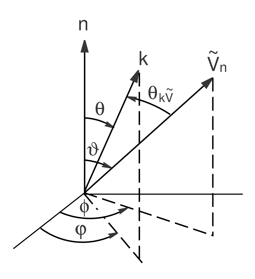
Figure 1: A sketch of the geometry and the different coordinate systems that are used to address the minimum energy state in a moving triplet-paired neutron condensate.

Than, by the addition theorem, the angle $\theta_{\mathbf{k\tilde{V}}}$ between the quasi-particle momentum and the flow direction can be written as

$$\cos\theta_{\mathbf{k\tilde{V}}}=\cos\vartheta\cos\theta+\sin\vartheta\sin\theta\cos\left(\varphi-\phi\right),$$ (44)

and the average over directions of the quasi-particle momentum is given by the integral

$$\left\langle\cdot\cdot\cdot\right\rangle=\frac{1}{4\pi}\int\sin\theta\,d\theta\,d\varphi\cdot\cdot\cdot.$$

In what follows we abbreviate the quantum numbers $M=0$ and $\left|M\right|=2$ as $M$. Taking into account the cylindrical symmetry of the anisotropic energy gap about the quantization axis: $\bar{b}_{M}^{2}(\mathbf{\hat{k})}=\bar{b}_{M}^{2}\left(\cos\theta\right)$, from Eq. (42) we obtain

$$\frac{\tilde{\Delta}_{M}^{\left(n\right)}}{T_{cn}} =\left[\frac{8\pi^{2}}{7\zeta\left(3\right)}\frac{5}{6}\frac{T_{cn}-T}{T_{cn}}\right.$$

$$\left.-\frac{5}{3}\frac{k_{Fn}^{2}}{T_{cn}^{2}}\allowbreak\tilde{V}_{n}^{2}\,\,\left(K_{1}^{\left(M\right)}\cos^{2}\vartheta+K_{2}^{\left(M\right)}\sin^{2}\vartheta\right)\right]^{1/2},$$ (45)

where

$$K_{1}^{\left(M\right)}=\int_{0}^{1}d\left(\cos\theta\right)\,\bar{b}_{M}^{2}\left(\cos\theta\right)\cos^{2}\theta\,$$ (46)

and

$$K_{2}^{\left(M\right)}=\frac{1}{2}\int_{0}^{1}d\left(\cos\theta\right)\,\bar{b}_{M}^{2}\left(\cos\theta\right)\sin^{2}\theta\,$$ (47)

When obtaining Eq. (45) the fact is used that $\left\langle\bar{b}_{M}^{4}(\mathbf{\hat{k})}\right\rangle=6/5$ in both the cases $M=0$ and $\left|M\right|=2$.

In order to choose the most favourable state of the moving condensate, it is necessary to estimate the free energy of the superfluid flow. The kinetic part of the free energy of the flow is the same for the ³P₂ states with $M=0$ and $\left|M\right|=2$. Therefore one has to consider only the internal part of the free energy excess, that is, the difference between the free energy of the superfluid state $F_{\mathtt{s}}$ and that of the normal state $F_{\mathtt{norm}}$. The corresponding expression for the case of spin-singlet pairing was obtained in Abrikosov et al. (1965). Following this work in the case of spin-triplet pairing for $T-T_{cn}\ll T_{cn}$, we get

$$F_{s}-F_{\mathtt{norm}}=-\left(\frac{k_{F}m^{\ast}}{2\pi^{2}}\right)\frac{7\zeta\left(3\right)}{16\pi^{2}}\frac{\tilde{\Delta}^{4}}{T^{2}}\left\langle\bar{b}_{M}^{4}\right\rangle$$ (48)

This expression is very similar to that obtained for the case of isotropic spin-singlet pairing, except of the factor $\left\langle\bar{b}_{M}^{4}\right\rangle$, which is caused by the anisotropy of the energy gap in the ³P₂ state. As was mentioned above, this factor, $\left\langle\bar{b}_{M}^{4}\right\rangle=6/5$, is the same in both the cases, $M=0$ and $\left|M\right|=2$. As can be seen, the excess free energy is a monotonic function of the amplitude of the energy gap $\tilde{\Delta}$, whose dependence on the effective flow velocity is given in Eq. (45). A larger energy gap corresponds to a lower energy of the moving condensate.

It follows from Eq. (45) that the total energy is minimal for $\vartheta=0$ or $\pi$ if $K_{1}^{\left(M\right)}<K_{2}^{\left(M\right)}$, and for $\vartheta=\pi/2$ if $K_{1}^{\left(M\right)}>K_{2}^{\left(M\right)}$. For the pairing case with $\left|M\right|=2$ when $\bar{b}_{\left|M\right|=2}^{2}=(3/2)\sin^{2}\theta$ the simple integration yields

$$K_{1}^{\left(\left|M\right|=2\right)}=\frac{1}{5},~{}\ K_{2}^{\left(\left|M\right|=2\right)}=\frac{2}{5}.$$ (49)

For the pairing with $M=0$ when $\bar{b}_{M=0}^{2}=\left(1+3\cos^{2}\theta\right)/2$ one gets

$$K_{1}^{\left(M=0\right)}=\frac{7}{15},~{}\ K_{2}^{\left(M=0\right)}=\frac{4}{15}.$$ (50)

At fixed temperature the right-hand side of Eq. (45) depends on the effective velocity $\tilde{V}_{n}$ of superfluid neutrons and is a monotonic function of the angle $\vartheta$ between the quantization axis and the direction of the effective flow velocity. Figure 2 shows the dependence of the energy gap amplitude on the effective velocity $\tilde{V}_{n}$ for $\vartheta=0$ and $\vartheta=\pi/2$. The solid lines are prepared for a spin-triplet condensate with $\left|M\right|=2$, the dashed lines correspond to Cooper pairs with $M=0$. All the curves are plotted for the dimensionless temperature $\tau\equiv T/T_{cn}=0.95$.

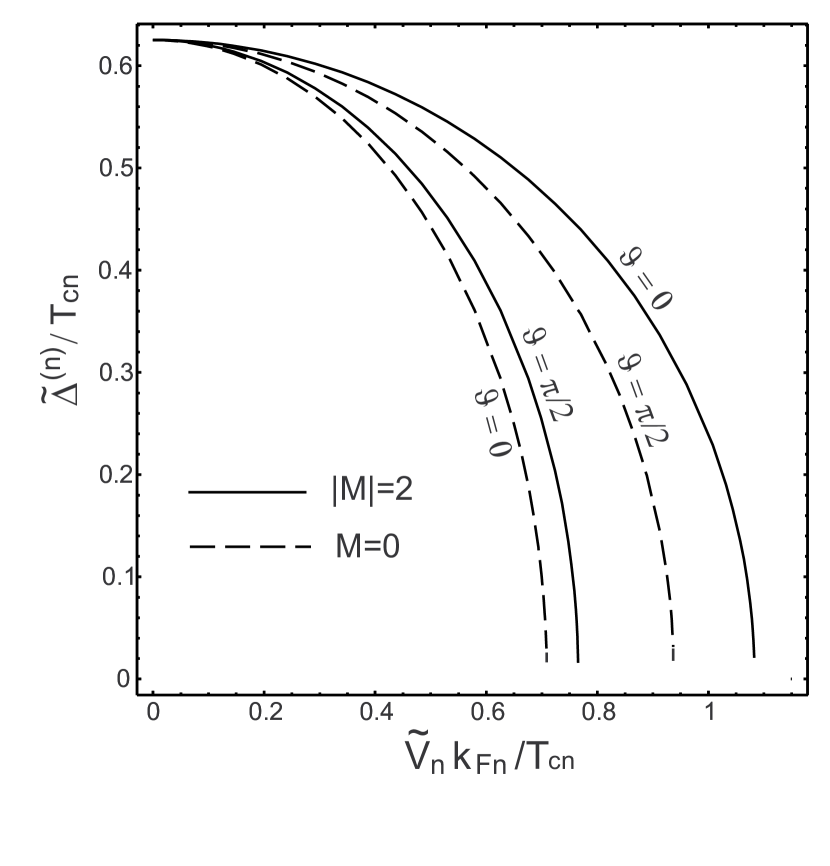
Figure 2: The dependence of the energy gap amplitude on the effective velocity $\tilde{V}_{n}$ for $\vartheta=0$ and $\vartheta=\pi/2$. The solid lines are prepared for a spin-triplet condensate with $\left|M\right|=2$, the dashed lines correspond to Cooper pairs with $M=0$. All the curves are plotted for the dimensionless temperature $\tau=0.95$.

As follows from this figure in an immovable superfluid liquid, all directions of the principal axis of the gap matrix are equivalent, because the corresponding states are degenerate. However, the superfluid motion eliminates the degeneration over the directions of the quantization axis. Moreover, states with $M=0$ and $\left|M\right|=2$, degenerate in an immovable superfluid liquid, are also split by a superfluid motion. The splitting of the energy levels rapidly increases with the increase in the effective flow velocity.

From this figure one may conclude:

(1) At temperatures just below the critical temperature $T_{cn}$ the superfluid motion makes the condensate with $\left|M\right|=2$ more energetically favourable than the condensate with $M=0$.

(2) The largest gap amplitude (the lowest flow energy) is realised when the quantization axis is directed along the superfluid flow velocity.

Since at the fixed velocity the pairing always occurs into the state of lowest energy, in what follows, we focus on the spin-triplet condensation with $\left|M\right|=2$ assuming that the quantization axis is directed along the flow direction. This justifies the general form (8) of the correction to the quasi-particle energy caused by the motion in superfluid neutron-proton mixture.

At lower temperatures such that $T_{cn}-T\sim T_{cn}$ the physical picture is more complicated. As, at zero temperature, the ground state with $M=0$ is preferable for a superfluid condensate at rest (see Appendix B) one can expect that, at lower temperatures, there exists some domain of the superfluid velocities and temperatures, where the state with $M=0$ has the lowest energy. Fig. 3 shows the dependence of the energy gap amplitude on the effective velocity $\tilde{V}_{n}$ at different temperatures $\tau$ for a moving condensate with $\left|M\right|=2$ and $\vartheta=0$ (the quantization axis along the flow velocity) and for the competitive superfluid state with $M=0$ and $\vartheta=\pi/2$, when the quantization axis is perpendicular the flow velocity.

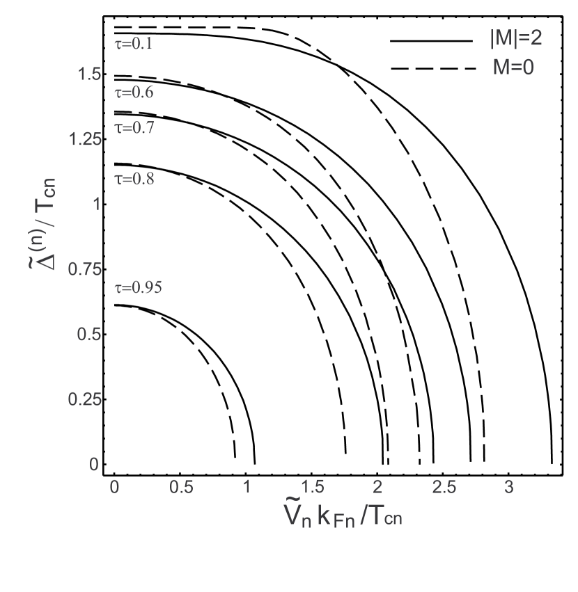
Figure 3: The energy gap amplitude against the effective velocity $\tilde{V}_{n}$ at different temperatures $\tau$ for a moving condensate with $\left|M\right|=2$ and $\vartheta=0$ (the quantization axis along the flow velocity) and for the competing superfluid state with $M=0$ and $\vartheta=\pi/2$ (the quantization axis is perpendicular the flow velocity),

Numerical estimates show a strong competition of the ³P₂ states with $M=0$ and $|M|=2$, which takes place near small superfluid velocities below the temperature about $(0.6\div 0.7)T_{cn}$. Let us notice that, in these domain of temperatures and superfluid velocities, the energy difference of the competing states of the triplet condensate does not exceed two percent, and the change of the gap value due to the superfluid motion is relatively small. We therefore restrict our analysis to the neutron condensation into the ³P${}_{2}(|M|=2)$ state at arbitrary temperatures below $T_{cn}$. We assume also that the quantization axis is directed along the superfluid flow velocity, as it follows from the above arguing.

4 A superfluid neutron-proton mixture with supercurrents.

4.1 Case of $(T_{cn}-T)/T_{cn}<<1$

For temperatures just below the critical temperature for the neutron superfluidity onset one can derive the analytic solution to the non-linear equations for the entrainment matrix. At temperatures near $T_{cn}$, such that $\left(\mathbf{k\tilde{V}}_{n}/T\right)^{2}\ll 1$ and $\left(\tilde{\Delta}^{\left(n\right)}\left(T\right)/T\right)^{2}\ll 1$, one can expand in a series in these small parameters the distribution functions under the integral in Eq. (24) to obtain

$$\tilde{\Phi}_{n}=3\int\frac{d\mathbf{\hat{k}}}{4\pi}\left(\mathbf{\hat{k}\hat{V}}_{n}\right)^{2}\left(1+7\zeta^{\prime}\left(-2\right)\frac{\tilde{\Delta}^{\left(n\right)2}}{T_{cn}^{2}}\bar{b}^{2}\left(\mathbf{\hat{k}}\right)\right),$$ (51)

where $\bar{b}^{2}=3/2\sin^{2}\theta$ and $\mathbf{\hat{V}}_{n}$ is a unit vector in the direction of the effective velocity of the neutron superfluid flow, so that $\mathbf{\hat{k}}\mathbf{\hat{V}}_{n}=\cos\theta$.

After performing the trivial integration over the solid angle we get

$$\tilde{\Phi}_{n}=1+\frac{3}{5}7\zeta^{\prime}\left(-2\right)\frac{\tilde{\Delta}^{\left(n\right)2}\left(T\right)}{T_{cn}^{2}}.$$ (52)

To obtain a consistent solution, we must substitute here the gap amplitude from Eq. (45) with $\vartheta=0$ and with $K_{1}^{\left(\left|M\right|=2\right)}$ and $K_{2}^{\left(\left|M\right|=2\right)}$ from Eq (49):

$$\frac{\tilde{\Delta}_{|M|=2}^{\left(n\right)2}}{T_{cn}^{2}}=\frac{8\pi^{2}}{7\zeta\left(3\right)}\frac{5}{6}\frac{T_{cn}-T}{T_{cn}}-\frac{1}{3}\frac{k_{Fn}^{2}}{T_{cn}^{2}}\allowbreak\tilde{V}_{n}^{2}.$$ (53)

Making use of the identity

$$\zeta^{\prime}\left(-2\right)\frac{8\pi^{2}}{\zeta\left(3\right)}=-2,$$ (54)

and combining Eqs. (52), (53) and (45) we find

$$\tilde{\Phi}_{n}=1-\left(1-\tau\right)\left(1-\frac{\tilde{V}_{n}^{2}}{V_{n\max}^{2}}\right),$$ (55)

where $\tau=T/T_{cn}$, and the maximal effective velocity is

$$V_{n\max}=\sqrt{\frac{20\pi^{2}}{7\zeta\left(3\right)}\left(1-\tau\right)}\frac{T_{cn}}{k_{Fn}}.$$ (56)

Making use of Eq. (102) we find

$$T_{cn}=\Delta_{0}^{\left(n\right)}\frac{\sqrt{6}}{\pi}e^{C-5/6}\simeq 0.6034\Delta_{0}^{\left(n\right)}.$$ (57)

This allows us to write the maximal effective velocity in the form

$$V_{n\max}=\sqrt{\frac{120e^{2C-5/3}}{7\zeta\left(3\right)}\left(1-\tau\right)}\upsilon_{n}^{cr},$$ (58)

where

$$\upsilon_{n}^{cr}=\frac{\Delta_{0}^{\left(n\right)}}{k_{Fn}}.$$ (59)

In Eq. (55), the function $\tilde{\Phi}_{n}$ has written in terms of the effective velocity of neutrons $\mathbf{\tilde{V}}_{n}$. To calculate the entrainment matrix we need this function in terms of the superfluid velocity of neutrons $\bm{v}_{n}$. To derive this function let us combine the equation

$$\mathbf{\tilde{V}}_{n}=\mathsf{\tilde{\gamma}}_{nn}\bm{v}_{n}+\mathsf{\tilde{\gamma}}_{np}\bm{v}_{p},$$ (60)

which follows from Eq. (7) with Eq. (41) to obtain

$$\mathbf{\tilde{V}}_{n}=\frac{1}{\mathsf{\tilde{\gamma}}_{pp}}\left(\mathsf{\tilde{\gamma}}_{nn}\mathsf{\tilde{\gamma}}_{pp}-\mathsf{\tilde{\gamma}}_{np}\mathsf{\tilde{\gamma}}_{pn}\right)\bm{v}_{n}.$$ (61)

Here the functions $\mathsf{\tilde{\gamma}}_{ab}$ are defined in the equations (21) - (23), where one has to put $\tilde{\Phi}_{p}=0$.

We now use the fact that the function $(1-\tilde{\Phi}_{n})$ is small as $\left(1-\tau\right)\ll 1$ [see Eq. (55)]. Therefore, in Eq. (61) one can take $\tilde{\Phi}_{n}$ in the lowest (zero) order, by replacing $\tilde{\Phi}_{n}\rightarrow 1$. From Eq. (58) we thus obtain

$$\frac{\tilde{V}_{n}}{V_{n\max}}=\sqrt{\frac{7\zeta\left(3\right)e^{5/3-2C}}{120\left(1-\tau\right)}}\frac{m_{n}}{m_{n}^{\ast}}\frac{v_{n}}{\upsilon_{n}^{cr}}.$$ (62)

Substituting this expression in Eq. (55) we obtain the function

$$\tilde{\Phi}_{n}\simeq\tau+\left(1-\tau\right)\left(\frac{v_{n}}{v_{n}^{\max}}\right)^{2},~{}v_{n}<v_{n}^{\max},$$ (63)

and $\tilde{\Phi}_{n}=1$ if $v_{n}\geq v_{n}^{\max}$, where

$$v_{n}^{\max}=\frac{m_{n}^{\ast}}{m_{n}}\sqrt{\frac{120\left(1-\tau\right)}{7\zeta\left(3\right)e^{5/3-2C}}}\upsilon_{n}^{cr}$$ (64)

is the velocity of the superfluid flow at which the neutron superfluidity collapses at temperature $\tau$.

Further calculation can be done with the aid of Eqs. (21)-(23) and (30), where one has to put $\tilde{\Phi}_{p}=0$, as the superfluid protons are considered in the low-temperature limit. We thus obtain

$${\rho}_{nn}=\rho_{n}\,\mathsf{\tilde{\gamma}}_{nn}\,\left(1-\tilde{\Phi}_{n}\right),~{}\ {\rho}_{pp}=\rho_{p}\,\mathsf{\tilde{\gamma}}_{pp}\,,$$ (65)

and

$${\rho}_{pn}={\rho}_{np}=\rho_{n}\,\mathsf{\tilde{\gamma}}_{np}\,\left(1-\tilde{\Phi}_{n}\right),$$ (66)

where

$$\mathsf{\tilde{\gamma}}_{pp} = {\frac{m_{p}}{m_{p}^{\ast}}}\left(1+{\frac{F_{1}^{pp}}{3}}-\frac{1}{9}\frac{F_{1}^{pn}F_{1}^{np}\tilde{\Phi}_{n}}{1+\,\tilde{\Phi}_{n}F_{1}^{nn}/3}\right)$$ (67)

$$\mathsf{\tilde{\gamma}}_{nn} = {\frac{m_{n}}{m_{n}^{\ast}}\frac{1+F_{1}^{nn}/3}{1+\,\tilde{\Phi}_{n}F_{1}^{nn}/3}}$$ (68)

$$\mathsf{\tilde{\gamma}}_{np} = {\frac{m_{p}}{\sqrt{m_{n}^{\ast}\,m_{p}^{\ast}}}}\left({\frac{k_{Fp}}{k_{Fn}}}\right)^{3/2}{\frac{\,F_{1}^{np}/3}{1+\,\tilde{\Phi}_{n}F_{1}^{nn}/3}}\,.\,\,\,$$ (69)

4.2 General case

Calculation of the non-linear entrainment matrix at arbitrary temperature of the mixture of superfluid nucleons to require numerical computations. Let us write the function $\tilde{\Phi}_{n}$ and the gap equation, defined in Eqs. (24) and (34) as

$$\tilde{\Phi}_{n}=\frac{3}{k_{Fn}\tilde{V}_{n}}\int\frac{d\mathbf{\hat{k}}}{4\pi}\int_{0}^{\infty}d\xi\left(\mathcal{\tilde{F}}_{-}^{\left(n\right)}-\mathcal{\tilde{F}}_{+}^{\left(n\right)}\right)\cos\theta,$$ (70)

$$\ln\frac{\Delta_{0}^{\left(n\right)}}{\tilde{\Delta}^{\left(n\right)}}=\int\frac{d\mathbf{\hat{k}}}{4\pi}\int_{0}^{\infty}d\xi\frac{\bar{b}^{2}(\mathbf{\hat{k}})}{\tilde{E}_{\mathbf{k}}^{\left(n\right)}}\left(\mathcal{\tilde{F}}_{+}^{\left(n\right)}+\mathcal{\tilde{F}}_{-}^{\left(n\right)}\right),$$ (71)

where the distribution functions and the bogolon energy are of the form

$$\mathcal{\tilde{F}}_{\pm}^{\left(n\right)}=\frac{1}{1+e^{\left(\tilde{E}_{\mathbf{k}}^{\left(n\right)}\pm k_{Fn}\tilde{V}_{n}\cos\theta\right)/T}},$$ (72)

and

$$\tilde{E}_{\mathbf{k}}^{\left(n\right)}=\sqrt{\xi^{2}+\tilde{\Delta}^{\left(n\right)2}\bar{b}^{2}},$$ (73)

respectively. Since the quantization axis $\mathbf{n}$ to be directed along the effective velocity $\mathbf{\tilde{V}}_{n}$, in Eq. (72) it is assumed $\theta\equiv\theta_{\mathbf{\hat{k}\tilde{V}}_{n}}=\theta_{\mathbf{\hat{k}n}}$.

Let us remind that the ³P₂ states with $M=0$ and $|M|=2$, are very close to one other below the temperature about $(0.6\div 0.7)T_{cn}$ when the superfluid velocity substantially smaller the critical value. The change of the gap value due to the superfluid motion in this domain is relatively small. Therefore it is sufficient to restrict our analysis to the neutron condensation into the ³P${}_{2}(|M|=2)$ state at arbitrary temperatures below $T_{cn}$.

The advantage of Eqs. (70) and (71) is that their solution $\tilde{\Phi}_{n}\left(T\right)$ is a function of the temperature $T$ and absolute value of the effective velocity $\tilde{V}_{n}$, which (at this stage of calculations) can be considered as external parameters. Self-consistent numerical solutions to these equations are depicted in Fig. 4 by solid curves. The function $\tilde{\Phi}_{n}$ is plotted against $\tilde{V}_{n}$ for a set of dimensionless temperatures $\tau=T/T_{cn}$, ranging from $0$ to $1$.

The function $\tilde{\Phi}_{n}\left(T\right)$ is independent explicitly of the Landau parameters. For practical calculations this function can be fitted by the expressions:

$$\tilde{\Phi}_{n}=f+\frac{g\,\left(1-f\right)\left(\tilde{V}_{n}/V_{\max}\right)^{2}}{1+\left(g-1\right)\left(\tilde{V}_{n}/V_{\max}\right)^{3/2}},~{}\ \tilde{V}_{n}<V_{\max}$$ (74)

and

$$\tilde{\Phi}_{n}=1,~{}\ \tilde{V}_{n}\geq V_{\max},$$ (75)

where

$$f=\frac{2.3197\tau^{2}\exp\left(0.0082\sqrt{1-\tau}+0.4829\tau\right)}{1+0.0788\tau+2.6808\tau^{2}},$$ (76)

$$g=\frac{2.9699+0.7847\tau+1.9295\tau^{2}}{1+0.4844\tau+5.1598\tau^{2}}.$$ (77)

The maximum effective velocity possible for the superfluid flow at the temperature $\tau$ can be found from Eq. (71) in the limit $\tilde{\Delta}^{\left(n\right)}\rightarrow 0$. In units of $\Delta_{0}^{(n)}/k_{Fn}$, it varies from $V_{\max}=\sqrt{3e/2}$ at $\tau=0$ to zero at $\tau=1$, see Leinson (2017), and can be fitted as

$$V_{\max}=2.0702\left(1-\tau^{2}\right)^{1/2}-0.051\left(1-\tau^{2}\right)^{2}.$$ (78)

Figure 4: The function $\tilde{\Phi}_{n}$ vs the dimensionless effective velocity at different temperatures indicated near the curves in units $\tau=T/T_{cn}$. Solid curves are as calculated numerically from a self-consistent solution of Eqs. (70) and (71). The dashed lines are computed from the fit presented in Eqs.(74)-(78).

Dashed lines in Fig. 4 show the fitted function $\tilde{\Phi}_{n}$. As can be seen the fit describes the curves with a good accuracy, so one can use it for a calculation of the entrainment matrix in superfluid nucleon mixtures with an arbitrary set of the Landau parameters. We now focus on this calculation.

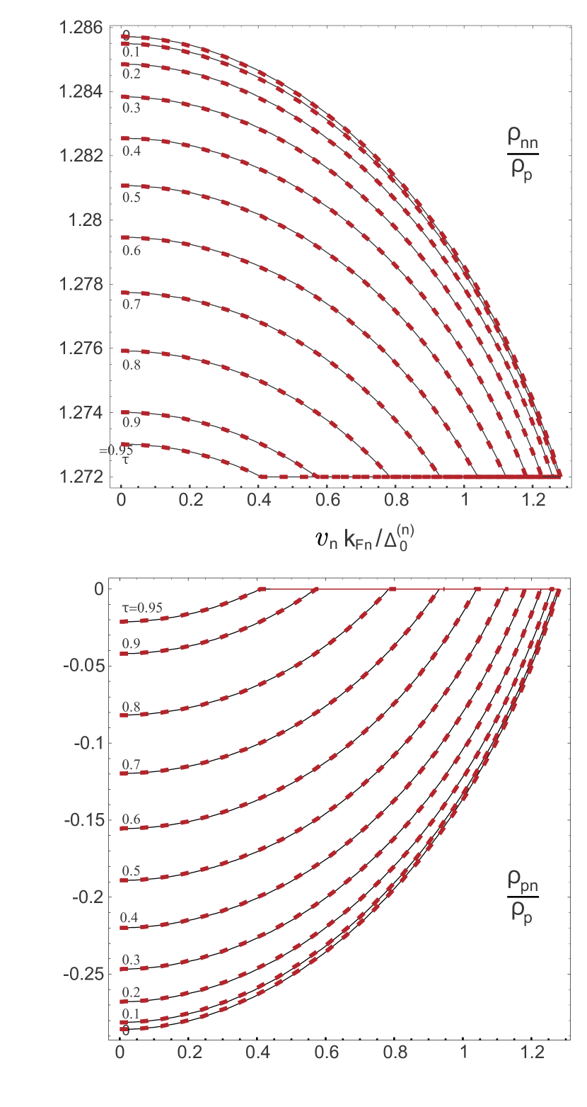
Figure 5: The components of the entrainment matrix as functions of the neutron superfluid flow velocity $v_{n}$ in the mixture of ¹S₀ superfluid protons and ³P${}_{2}(|M|=2)$ superfluid neutrons for different temperatures indicated near the curves in units $\tau=T/T_{cn}$. The superfluid flow velocity is indicated in units of the critical velocity $\Delta_{0}^{(n)}/k_{Fn}$. Solid curves demonstrate the exact numerical result. The curves obtained with the aid of the fitted expressions (74)-(78) are shown in dashed lines.

As we consider the proton superfluid in the low-temperature limit, the entrainment matrix is given by Eqs. (21)-(23) and (30), with $\tilde{\Phi}_{p}=0$. In this case, the right sides of these equations depend on the temperature and effective velocity $\mathbf{\tilde{V}}_{n}$ of neutrons. We, however, need the dependence of the entrainment matrix on the superfluid velocity $\bm{v}_{n}$.

To this end let us combine Eq. (60), with Eq. (41) to obtain the superfluid velocity $\bm{v}_{n}$ as a function of the effective velocity $\mathbf{\tilde{V}}_{n}$. Making also use of Eqs. (21)-(23) and (30) with $\tilde{\Phi}_{p}=0$ we finally get

$$v_{n}={\frac{m_{n}^{\ast}}{m_{n}}}\frac{\left(1+\,\tilde{\Phi}_{n}\,F_{1}^{nn}/3\right)\,\left(1+F_{1}^{pp}/3\,\right)-\,\tilde{\Phi}_{n}\,F_{1}^{np}F_{1}^{pn}/9}{\left(1+F_{1}^{pp}/3\right)\left(1+F_{1}^{nn}/3\,\right)-F_{1}^{pn}F_{1}^{np}/9}\tilde{V}_{n},$$ (79)

$$\frac{{\rho}_{nn}}{\rho_{n}} = {\frac{m_{n}}{m_{n}^{\ast}}\frac{1+F_{1}^{nn}/3}{1+\,\tilde{\Phi}_{n}F_{1}^{nn}/3}}(1-\tilde{\Phi}_{n})$$ (80)

$$\frac{{\rho}_{np}}{\rho_{n}} = {\frac{m_{p}}{\sqrt{m_{n}^{\ast}\,m_{p}^{\ast}}}}\left({\frac{k_{Fp}}{k_{Fn}}}\right)^{3/2}{\frac{\left(1-\tilde{\Phi}_{n}\right)\,F_{1}^{np}/3}{1+\,\tilde{\Phi}_{n}F_{1}^{nn}/3}}\,\,,\,\,$$ (81)

and $\rho_{np}=\rho_{pn}$. Since we consider the proton superfluid in the low-temperature limit the $\rho_{pp}$ matrix element can be obtained from the identity due to Galilean invariance

$$\rho_{pp}+\rho_{pn}=\rho_{p}.$$

The right sides of Eqs. (79), (80) and (81) depend on the temperature and effective velocity $\tilde{V}_{n}$ which can take the values between $0$ and $V_{\max}(\tau)$. The Eq. (79) in a pair with each of Eqs. (80) and (81) allows one to get the parametric curves ${\rho}_{ab}(v_{n},T)$ employing $\tilde{V}_{n}$ as a parameter.

For illustration, of the temperature and supercurrents effects on the entrainment efficiency in the neutron star core we have considered a superfluid nucleon liquid with a total density of baryons $n_{b}=n_{n}+n_{p}=2n_{0}$, where $n_{0}=0.16$ fm^-3 is the normal nuclear density. We use realistic parameters obtained with the use of APR equation of state (Akmal et al., 1998) in many calculations of a NS with the mass $1.4M_{\odot}$ (see, e.g. Gualtieri et al., 2014). Assuming the nucleon matter in beta-equilibrium the asymmetry parameter $\delta=(n_{n}-n_{p})/n_{b}$ is adopted to be $\delta=0.7$. Following Gusakov et al. (2013) we employ the density-dependent model for spin-singlet pairing of protons and spin-triplet pairing for neutrons in the NS core. This model is in agreement with microscopic calculations (see, e.g. Yakovlev et al., 1999a) and is similar to the model of nucleon pairing used in cooling simulations of the NS in Cassiopea A supernova remnant (Shternin et al., 2011). For $n_{b}=2n_{0}$ this model suggests the critical temperatures for the proton and neutron superfluidity onset $T_{cp}=6\times 10^{9}\,\mathsf{K}$ and $T_{cn}=5\times 10^{8}\,\mathsf{K}$, respectively.

Information on the Landau parameters for asymmetric nuclear matter is very limited. We use the density-dependent Landau parameters obtained microscopically in Gusakov et al. (2009b), which turn out to be $F_{1}^{nn}=-1$, $F_{1}^{pp}=-0.3$, $F_{1}^{np}=F_{1}^{pn}=-0.24$ for $n_{b}=2n_{0}$.

The components of the entrainment matrix $\rho_{nn}$ and $\rho_{pn}$, as functions of the superfluid velocity $v_{n}$ of the neutron flow, are depicted in Fig. 5. Solid curves demonstrate the exact numerical result. The curves obtained with the aid of the fitted expressions (74)-(78) are shown in dashed lines. The $\rho_{pp}$ component of the entrainment matrix is almost independent of the velocities of superfluid flows because the Eq. (41) insures that the velocity of superfluid protons is small in comparison with its critical value

$$v_{p}\sim v_{n}<\Delta_{0}^{\left(n\right)}/k_{Fn}\ll\Delta_{0}^{\left(p\right)}/k_{Fp}.$$

This means that the the superfluid energy gap of protons remains constant at this motion. In the considered case we got $\rho_{pp}=1.285\rho_{p}$.

Let us notice that the function $\tilde{\Phi}_{n}$, defined in Eq. (70) and fitted by the expressions (74)-(78) universally depends on only the dimensionless temperature $\tau$ and parameter $k_{Fn}\tilde{V}_{n}/\Delta_{0}^{\left(n\right)}$. This function can be applied for any density of superfluid neutrons and any model of the ³P₂ neutron pairing. Thus, a change of the entrainment matrix $\rho_{ab}$, as the function of the temperature and parameter $k_{Fn}\tilde{V}_{n}/\Delta_{0}^{\left(n\right)}$, can be caused by only a varying of the Landau parameters and the effective nucleon masses along with the density change. To get an idea about the range of this changes let us calculate the entrainment matrix for the nucleon density $n=3n_{0}$ in the same model assumptions. In this case we take the asymmetry parameter in beta-equilibrium to be $\delta=0.837$, the critical temperatures for the proton and neutron superfluidity onset $T_{cp}=5\times 10^{9}\,\mathsf{K}$ and $T_{cn}=6\times 10^{8}\,\mathsf{K}$, respectively, and the Landau parameters $F_{1}^{nn}=-1$, $F_{1}^{pp}=-0.55$, $F_{1}^{np}=F_{1}^{pn}=-0.3$.

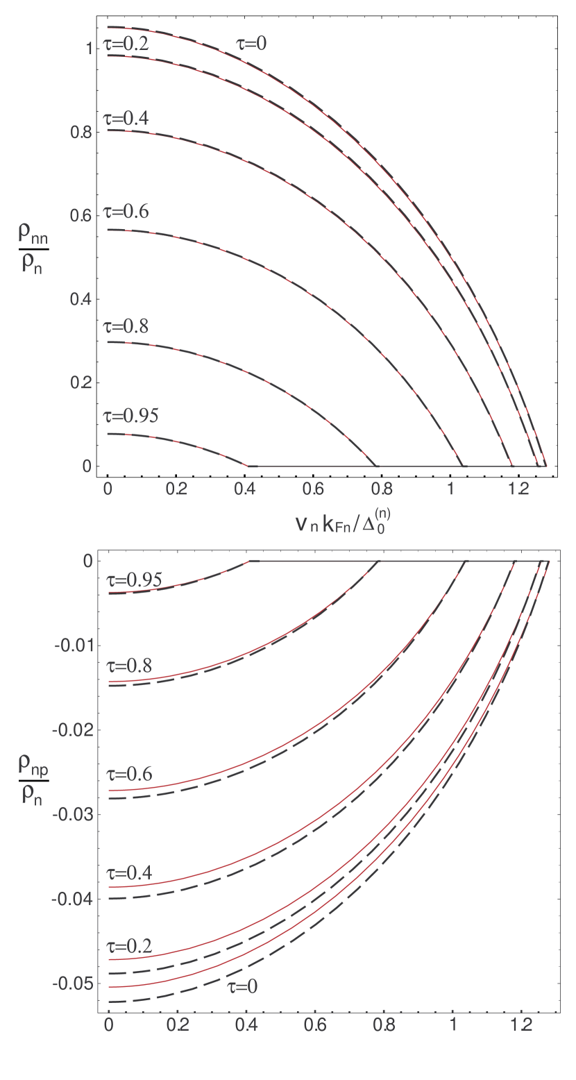
Figure 6: The components of the entrainment matrix $\rho_{nn}$ and $\rho_{np}$, as functions of the superfluid velocity $v_{n}$ of the neutron flow. Solid curves correspond to $n=2n_{0}$. The dashed lines are same but for the baryon density $n_{b}=3n_{0}$.

The result of this calculation is depicted in Fig. 6. For a comparison we show the curves calculated for $n_{b}=3n_{0}$ together with the results of the previous calculation for $n_{b}=2n_{0}$. One can see that the $\rho_{nn}$ component of the entrainment matrix is practically unchanged with the density increase, while the $\rho_{np}$ (and consequently $\rho_{pn}$) have slightly changed. Maximal change is about $4\%$

5 Summary

We considered the entrainment effect in a warm mixture of superfluid baryons in the core of an oscillating neutron star with an internal temperature below the critical temperature $T_{cn}$ for the onset of neutron superfluidity. It is assumed that the critical temperature for Cooper pairing of protons $T_{cp}$ is substantially higher than that for neutrons and thus protons are also superfluid. The suggested theory takes into account the entrainment dependence on the superfluid velocities and temperature. The velocity dependence of the entrainment matrix is caused by a strong suppression of the superfluid energy gaps by supercurrents. Recently this effect was considered for the superfluid mixture of nucleons at zero temperature (Leinson, 2017). Calculations that also take into account temperature effects are proposed in the present work for the first time.

A closed system of non-linear equations for the entrainment matrix is considered taking into account the dependence of the superfluid gap on the temperature and velocities of superfluid nucleons. Below the critical temperature $T_{cn}$, the entrainment matrix can be completely described by the Landau parameters and function $\tilde{\Phi}_{n}$ which universally depends on only the dimensionless temperature $\tau$ and parameter $k_{Fn}\tilde{V}_{n}/\Delta_{0}^{\left(n\right)}$. This function has been calculated numerically and fitted by simple formulas convenient for a practical use. It can be applied for any density of superfluid neutrons and any model of the ³P₂ neutron pairing.

The simple procedure is suggested for a construction of the entrainment matrix for arbitrary set of the Landau parameters $F_{1}^{nn}$, $F_{1}^{pp}$ and $F_{1}^{np}=F_{1}^{pn}$ with the aid of the fitted function $\tilde{\Phi}_{n}$ . The entrainment matrix, calculated in this way, is shown together with the exact numerical solution in Fig. 5, which demonstrates very good agreement.

From the plots it is seen also the strong dependence of the entrainment efficiency on the temperature and the neutron superfluid velocity. The value of superfluid velocity at which the neutron superfluidity is destroyed and the entrainment disappears crucially depends on the temperature and becomes very small at temperatures just below the critical value $T_{cn}$. This effect significantly distinguishes our result from the entrainment matrix derived in Gusakov & Haensel (2005), where the energy gaps and, consequently, the entrainment matrix are assumed be independent of the superfluid velocities.

Let us notice that the simple expressions for a calculation of the entrainment matrix fitted in Eqs. (74)-(78) of the present work are valid for any temperature below $T_{cn}$ and can be employed also for the case of very low temperature by substituting $\tau=0$. This limiting case is important for the most neutron stars older then $\sim 10^{5}$ years. However, for oscillations of young neutron stars at the cooling epoch one has to take into consideration the temperature impact (see, e.g. Gusakov & Andersson, 2006).

The entrainment effect plays very important role in NS pulsations dynamics (Prix, 2004; Carter et al., 2005; Chamel & Carter, 2006). Due to the complicated dependence on superfluid velocities, the entrainment matrix will become a non-linear function of the oscillation amplitude. Owing to the temperature effects, considered in the paper, the non-linearity will affect the pulsations in the warm superfluid mixture of nucleons at lower amplitudes than it takes place at zero temperature. The reduction of the neutron gap due to joint impact of the superfluid velocity and temperature should greatly influence the eigenfrequencies and eigenfunctions of oscillating NS. This will also influence the dissipation processes, because bulk viscosity of the nucleon superfluid mixture explicitly depends on the entrainment matrix (Alford et al., 2012). The dependence of the entrainment matrix on temperature and on superfluid velocities is important for mutual friction and related phenomena. The potential possibility of these effects has already been noted in the work by Gusakov & Kantor (2013).

In addition, one can expect that the destruction of neutron superfluidity caused by the critical supercurrents in oscillating neutron stars should alternate with the subsequent condensation of superfluid neutrons in the comoving reference frame (in our case in the rest frame). Indeed, as we have discussed, the destruction of the neutron superfluidity results in the bogolons forming the normal liquid, which should be unstable with respect to Cooper pairing. As can be seen from Fig. 3, below the critical temperature, the neutron liquid is the most unstable to the condensation with the effective velocity $\mathbf{\tilde{V}}_{n}=0$, which corresponds to the superfluid velocity $\bm{v}_{n}=-(\rho_{np}/\rho_{nn})\bm{v}_{p}$. Under the influence of the pressure gradient and the force of gravity, the newly created superfluid liquid will be accelerated to the critical velocity and again destroyed. This new regime of oscillations has not been discussed in the literature and deserves a separate study.

Appendix A Single-particle Green function in a superfluid flow of fermions

Consider a fermion system described by the following Hamiltonian with pairing (For brevity, the volume of the system is set to $\Omega=1$.)

$$\mathcal{H} =\sum_{\mathbf{k}\alpha}\xi_{\mathbf{k}}a_{\mathbf{k}\alpha}^{\dagger}a_{\mathbf{k}\alpha}$$

$$+ \frac{1}{2}\sum_{\begin{subarray}{c}\mathbf{k}_{1}\alpha,\mathbf{k}_{2}\beta,\\ \mathbf{k}_{3}\gamma,\mathbf{k}_{4}\delta\end{subarray}}\left\langle\mathbf{k}_{1}\alpha,\mathbf{k}_{2}\beta\left|U\right|\mathbf{k}_{4}\delta,\mathbf{k}_{3}\gamma\right\rangle a_{\mathbf{k}_{1}\alpha}^{\dagger}a_{\mathbf{k}_{2}\beta}^{\dagger}a_{\mathbf{k}_{3}\gamma}a_{\mathbf{k}_{4}\delta}$$ (82)

where the Greek letters denote spin indices; $\xi_{\mathbf{k}}=p^{2}/2m-\mu$ and $\mu$ is the Fermi·energy of the system. Since the pairing interaction conserves the total momentum, its matrix element can be written in the form

$$\left\langle\mathbf{k}_{1}a,\mathbf{k}_{2}\beta\left|U\right|\mathbf{k}_{4}\delta,\mathbf{k}_{3}\gamma\right\rangle$$

$$=\delta_{\mathbf{k}_{1}+\mathbf{k}_{2},\mathbf{k}_{3}+\mathbf{k}_{4}}U_{\alpha\gamma,\beta\delta}\left(\frac{\mathbf{k}_{1}-\mathbf{k}_{2}}{2}\mathbf{,}\frac{\mathbf{k}_{4}-\mathbf{k}_{3}}{2}\right)$$ (83)

Consider the case where the center of mass of all the pairs are moving with velocity $\mathbf{v}_{s}$, that is, when there is a uniform flow of the superfluid. If the total momentum of a Cooper pair at the point $\mathbf{R=}\left(\mathbf{r}_{1}+\mathbf{r}_{2}\right)/2$ is $2\mathbf{Q}=2m\mathbf{v}_{s}$, the initial momenta of the pairing nucleons should be $\left(\mathbf{k}+\mathbf{Q},-\mathbf{k}+\mathbf{Q}\right)$ rather than with $\left(\mathbf{k},-\mathbf{k}\right)$. For this case the Gor’kov equations for the ordinary and anomalous Green’s functions have been derived in Fujita & Tsuneto (1972). In particular, the equation for the ordinary Green function is of the following form in the Matsubara representation

$$\left(i\omega_{r}-\xi_{\mathbf{k}^{+}}\right)\left(i\omega_{r}+\xi_{\mathbf{k}^{-}}\right)\mathcal{\tilde{G}}_{\alpha\beta}\left(\omega_{r},\mathbf{k}\right)-\sum_{\gamma\delta}\tilde{\Delta}_{\alpha\gamma}\left(\mathbf{\hat{k}}\right)$$

$$\times\tilde{\Delta}_{\gamma\delta}^{\dagger}\left(\mathbf{\hat{k}}\right)\mathcal{\tilde{G}}_{\delta\beta}\left(\omega_{r},\mathbf{k}\right)=\left(i\omega_{r}+\xi_{\mathbf{k}^{-}}\right)\delta_{\alpha\beta},$$ (84)

Here and below $\mathbf{\hat{k}}=\mathbf{k}/k$,

$$\omega_{r}=\left(2r+1\right)\pi T,~{}\ r=1,2,3,\cdot\cdot\cdot$$ (85)

is the fermion Matsubara frequency, and the tilde above a letter indicates values that depend on the velocity of the superfluid flow. The order parameter $\tilde{\Delta}_{\alpha\beta}$ represents a $2\times 2$ matrix in spin space $\left(\alpha,\beta=\uparrow,\downarrow\right)$, and

$$\xi_{\mathbf{k}^{\pm}}=\frac{\left(\mathbf{k}\pm m\mathbf{v}_{s}\right)^{2}}{2m}-\mu\simeq\xi_{k}\pm\mathbf{k}\mathbf{v}_{s}.$$ (86)

In obtaining this equality we have neglected the term $mv_{s}^{2}/2$ assuming $mv_{s}\ll k_{F}$, where the Fermi momentum is specified by the particle number density $N$ of the degenerate Fermi gas

$$k_{F}=\left(3\pi^{2}N\right)^{1/3}.$$ (87)

If we restrict our consideration to the case of a non rotating neutron star and consider the unitary states of the gap matrix then

$$\sum_{\gamma}\tilde{\Delta}_{\alpha\gamma}\left(\mathbf{\hat{k}}\right)\tilde{\Delta}_{\gamma\delta}^{\dagger}\left(\mathbf{\hat{k}}\right)=\delta_{\alpha,\delta}\tilde{D}^{2\,}\left(\mathbf{\hat{k}}\right),$$ (88)

where $\tilde{D}^{2\,}\left(\mathbf{\hat{k}}\right)$ is real, and Eq. (84) takes the simple form

$$\mathcal{\tilde{G}}_{\alpha\beta}\left(\omega_{r},\mathbf{k}\right)=\delta_{\alpha\beta}\frac{1}{2}\left(\frac{1+\xi_{k}/\tilde{E}_{\mathbf{k}}}{i\omega_{r}-\tilde{E}_{\mathbf{k}}-\mathbf{k}\mathbf{v}_{s}}+\frac{1-\xi_{k}/\tilde{E}_{\mathbf{k}}}{i\omega_{r}+\tilde{E}_{\mathbf{k}}-\mathbf{k}\mathbf{v}_{s}}\right),$$ (89)

where

$$\tilde{E}_{\mathbf{k}}=\sqrt{\xi_{k}^{2}{}+\tilde{D}^{2\,}\left(\mathbf{\hat{k}}\right)}.$$ (90)

The only change brought to these formulae by the supercurrent is that instead of $i\omega_{r}$ we have $i\omega_{r}-\mathbf{k}\mathbf{v}_{s}$, and the chemical potential is shifted as well: $\mu\rightarrow\mu-mv_{s}^{2}/2$.

Appendix B Spin-triplet pairing of neutrons

As is well known the spin-triplet neutron condensate arises in the high-density neutron matter mostly owing to the attractive spin-orbit and tensor interactions in the channel of two quasi-particles Takatsuka (1972). However, the tensor interactions are not very significant in the beta-stable baryon matter [see, e.g. Takatsuka (1972); Baldo et al. (1992); Elgaroy et al. (1996b); Khodel et al. (2001)]. Therefore to avoid cumbersome calculations we restrict our analysis to the case of neutron pairing in the unitary ³P₂ channel. In this case the energy gap

$$\tilde{D}_{\mathbf{\hat{k}}}=\tilde{\Delta}^{\left(n\right)}\bar{b}(\mathbf{\hat{k}})$$ (91)

depends on the direction of the quasi-particle momentum $\mathbf{\hat{k}=k}/k$ and, in general, has nodes. The amplitude of the energy gap $\tilde{\Delta}^{\left(n\right)}$ must be real up to an arbitrary overall phase factor. We, therefore, may adopt that the gap amplitude $\tilde{\Delta}^{\left(n\right)}$ is a real function which depends on the temperature $T$ and the effective flow velocity $\tilde{V}$_n. The gap anisotropy is determined by some vector $\mathbf{\bar{b}}(\mathbf{\hat{k}})$ in the spin space, which is chosen to be real in accordance to the unitary condition and is normalized by the condition

$$\int\frac{d\mathbf{\hat{k}}}{4\pi}\bar{b}^{2}(\mathbf{\hat{k}})=1~{}.$$ (92)

It should be noted that, by virtue of Eq. (92), the amplitudes $\Delta_{0}^{\left(n\right)}$ and $\tilde{\Delta}^{\left(n\right)}$ are chosen as to represent the energy gap averaged over the solid angle. Defined in this way, the average energy gap furnishes an overall measure of the pairing correction to the ground-state energy in the preferred state.

The equation that allows one to find the gap amplitude $\tilde{\Delta}^{\left(n\right)}$ as a function of the temperature and velocity $\tilde{V}$_n of the superfluid flow can be written in the form Fujita & Tsuneto (1972); Leinson (2017):

$$\frac{k_{Fn}m_{n}^{\ast}}{\pi^{2}}\ln\frac{\Delta_{0}^{\left(n\right)}}{\tilde{\Delta}^{\left(n\right)}}=\sum_{\mathbf{k}}\frac{\bar{b}^{2}(\mathbf{\hat{k}})}{\tilde{E}_{\mathbf{k}}^{\left(n\right)}}\left(\mathcal{\tilde{F}}_{+}^{\left(n\right)}+\mathcal{\tilde{F}}_{-}^{\left(n\right)}\right).$$ (93)

In this equation, $\Delta_{0}^{\left(n\right)}$ is the energy gap amplitude in the superfluid at rest (i.e. for $\tilde{V}$${}_{n}=0$) and temperature $T=0$. The distribution functions for the Bogoliubov excitations $\mathcal{\tilde{F}}_{\pm}^{\left(n\right)}$ are as defined in Eq. (14) with

$$\tilde{E}_{\mathbf{k}}^{\left(n\right)}=\sqrt{\xi_{k}^{\left(n\right)2}+\tilde{\Delta}^{\left(n\right)2}\bar{b}^{2}(\mathbf{\hat{k}})}.$$ (94)

Note that if one formally puts $\bar{b}\rightarrow 1$, the equation (34) becomes identical to Eq. (31).

The vector $\mathbf{\bar{b}}(\mathbf{\hat{k}})$ defines the angle anisotropy of energy gap which depends on the phase state of the superfluid condensate. In general form, this vector can be written as $\bar{b}_{i}=\bar{A}_{ij}\hat{k}_{j}$, where $\bar{A}_{ij}$ is a $3\times 3$ matrix. In the case of a unitary ³P₂ condensate this matrix must be a real symmetric traceless tensor. It may be specified by giving the orientation of its principal axes and its two independent diagonal elements in its principal-axis coordinate system.

In total, there are five matrices $\ A_{ij}^{\left(M\right)}$, in accordance with the five possible projections $M=0,\pm 1,\pm 2$ of the total angular momentum of a pair in the ³P₂ state. Since the ground state should be invariant under time reversal, the states with magnetic quantum numbers $\pm M$ must be populated with equal likelihood. This requirement yields the following five symmetric combinations

$$A^{\left(0\right)}=\frac{1}{\sqrt{2}}\left(\begin{array}[]{ccc}-1&0&0\\ 0&-1&0\\ 0&0&2\end{array}\right),$$ (95)

$$A^{\left(2\right)}+A^{\left(-2\right)}=\sqrt{\frac{3}{2}}\left(\begin{array}[]{ccc}1&0&0\\ 0&-1&0\\ 0&0&0\end{array}\right),$$ (96)

$$A^{\left(1\right)}-A^{\left(-1\right)}=-\sqrt{\frac{3}{2}}\left(\begin{array}[]{ccc}0&0&1\\ 0&0&0\\ 1&0&0\end{array}\right),~{}$$ (97)

$$A^{\left(2\right)}-A^{\left(-2\right)}=i\sqrt{\frac{3}{2}}\left(\begin{array}[]{ccc}0&1&0\\ 1&0&0\\ 0&0&0\end{array}\right),~{}$$ (98)

$$\ A^{\left(1\right)}+A^{\left(-1\right)}=-i\sqrt{\frac{3}{2}}\left(\begin{array}[]{ccc}0&0&0\\ 0&0&1\\ 0&1&0\end{array}\right).$$ (99)

On the other hand, the gap tensor $\bar{A}_{ij}$ should be diagonal, which excludes the possibility of populating states with $M=\pm 1$.  Therefore within the preferred coordinate system, there exist two simple solutions of Eq. (93) with $\bar{A}=A^{\left(0\right)}$ and with $\bar{A}=A^{\left(2\right)}+A^{\left(-2\right)}$. For the first solution, which represents a condensation of the pairs into the state with $M=0$, we have $\bar{b}_{M=0}^{2}(\mathbf{\hat{k}})=1/2\left(1+3\cos^{2}\theta\right)$. The second solution corresponds to $\left|M\right|=2$. In this case $\bar{b}_{\left|M\right|=2}^{2}(\mathbf{\hat{k}})=3/2\sin^{2}\theta$. The ³P₂ condensates, with $M=0$ and $\left|M\right|=2$, are known to be almost degenerate in the neutron superfluid at rest.

In Eq. (93), $\Delta_{0}^{\left(a\right)}$ is uniquely related to the temperature of the superfluid transition $T_{ca}$, which is assumed to be known, and $\tilde{\Delta}^{\left(a\right)}$ is the energy gap, which for a fixed density depends on the temperature and velocity $\tilde{V}$_a of the superfluid flow relative the normal (non-superfluid ) component.

The critical temperature for the onset of superfluidity can be found from Eq. (93) with the flow velocity equal to zero, $\tilde{V}$${}_{n}=0$. The summation on the right-hand side can be done with the aid of the formula

$$\int\frac{d^{3}k}{\left(2\pi\right)^{3}}\cdot\cdot\cdot=\frac{k_{F}m^{\ast}}{2\pi^{2}}\int\frac{d\mathbf{\hat{k}}}{4\pi}\int_{-\infty}^{\infty}d\xi_{k}\cdot\cdot\cdot.$$ (100)

Close to the transition point $T\rightarrow T_{cn}$, when $\Delta^{\left(n\right)2}/T^{2}\ll 1$, the equation with $\tilde{V}$${}_{n}=0$ takes the form

$$\ln\frac{\Delta_{0}^{\left(n\right)}}{T}=\ln\pi-C+\left\langle\bar{b}^{2}\ln\frac{1}{\bar{b}}\right\rangle+\frac{7\zeta\left(3\right)}{8\pi^{2}}\frac{\Delta^{\left(n\right)2}}{T^{2}},$$ (101)

where $C=0.577216$ - Euler’s constant, $\zeta\left(x\right)$ is the Riemann zeta function, $\zeta\left(3\right)=1.202$; and the angle brackets denote the average over directions of the quasi-particle momentum, as indicated in Eq. (43). Details of similar calculations can be found in Lifshitz & Pitaevskii (1980). Additionally the fact is used that $\left\langle\bar{b}^{2}\right\rangle=1$, according to the normalization condition (92). By Eq. (101) the gap vanishes at the temperature

$$T_{cn}=\Delta_{0}^{\left(n\right)}\frac{e^{C}}{\pi}\exp\left\langle\bar{b}^{2}\ln\bar{b}\right\rangle.$$ (102)

In the case of ³P₂ pairing with $M=0$ this equation gives $\Delta_{0}^{\left(n\right)}=1.\,\allowbreak 681T_{cn}~{}$while for $\left|M\right|=2$ one gets $\Delta_{0}^{\left(n\right)}=1.\noindent 657T_{cn}.$

Note that if one formally puts $\bar{b}$ equal to unity, the equation (102) recover the well-known results of the ¹S₀ pairing, presented in Eq. (33).

Figure 7: The temperature dependence of the energy gap in the superfluid at rest found from Eq. (93) with $\bm{v}_{n}=0$. The gap amplitudes $\Delta^{\left(n\right)}$ for a spin-triplet condensation with $M=0$ and $\left|M\right|=2$ are shown in units of the critical temperature $T_{cn}$ against the dimensionless temperature $\tau=T/T_{cn}$.

The temperature dependence of the energy gap in the superfluid at rest can be found from Eq. (93) with $\tilde{V}$${}_{n}=0$. Numerical solution to this equation is depicted in Fig. 7, where the energy gap amplitude $\Delta^{\left(n\right)}$ is shown in units of the critical temperature $T_{cn}$ versus the dimensionless temperature $\tau=T/T_{cn}$ for a spin-triplet condensation with $M=0$ and $\left|M\right|=2$. It can be seen that in an immovable superfluid liquid, the two condensate states have a very close energies. We can consider them degenerate in the temperature range just below the critical value.

References

- Abrikosov et al. (1965) Abrikosov A. A., Gor’kov L. P., Dzyaloshinski I. E., 1965, Methods of Quantum Field Theory in Statistical Physics, 2nd ed.. Pergamon Press
- Akmal et al. (1998) Akmal A., Pandharipande V. R., Ravenhall D. G., 1998, Phys. Rev. C58, 1804
- Alexandrov (2003) Alexandrov A. S., 2003, Theory of Superconductivity: From Weak to Strong Coupling. IOP publishing. Bristol & Philadelphia
- Alford et al. (2012) Alford M. G., Reddy S., Schwenzer K., 2012, Phys. Rev. Lett. 108, 111102
- Alpar et al. (1984) Alpar M. A., Langer S. A., Sauls J. A., 1984, Astrophys. J. 282, 533
- Andersson (1958) Andersson P. V., 1958, Phys. Rev. 112, 1900
- Andersson (1998) Andersson N., 1998, ApJ, 502, 708
- Andersson & Itoh (1975) Andersson P. V., Itoh N., 1975, Nature, 256, 25
- Andersson & Kokkotas (2001) Andersson N., Kokkotas K. D., 2001, Int. J. of Modern Phys. D10, 381
- Andersson et al. (1999) Andersson N., Kokkotas K. D., Stergioulas N., 1999, Astrophys. J. 516, 307
- Andersson et al. (2003) Andersson N., Comer G. L., Prix R., 2003, Phys. Rev. Lett. 90, 091101
- Andreev & Bashkin (1975) Andreev A. F., Bashkin E. P., 1975, Zh. Exp. Teor. Fiz. 69, 319
- Arras et al. (2003) Arras P., Flanagan E. E., Morsink S. M., Schenk A. K., Teukolsky S. A., Wasserman I., 2003, ApJ, 591, 1129
- Baldo et al. (1992) Baldo M., Cugnon J., Lejeune A., Lombardo U., 1992, Nucl. Phys. A536 and349
- Bardeen (1962) Bardeen J., 1962, Rev. of Modern Phys. 34, 667
- Borumand et al. (1996) Borumand M., Joynt R., Kluźniak W., 1996, Phys. Rev. C, 54, 2745
- Brown et al. (2017) Brown E. F., Cumming A., Fattoyev F. J., Horowitz C. J., Page D., Reddy S., 2017, Phys. Rev. Lett. 120 , 182701
- Caillon et al. (2001) Caillon J. C., Gabinski P., Labarsouque J., 2001, Nucl. Phys. A, 696, 623
- Caillon et al. (2002) Caillon J. C., Gabinski P., Labarsouque J., 2002, J. Phys. G, 28, 189
- Caillon et al. (2003) Caillon J. C., Gabinski P., Labarsouque J., 2003, J. Phys. G, 29, 2291
- Carter et al. (2005) Carter B., Chamel N., Haensel P., 2005, Nucl. Phys. A, 748, 675
- Chamel & Carter (2006) Chamel N., Carter B., 2006, Mon. Not. Roy. Astron. Soc. 368, 796
- Chamel & Haensel (2006) Chamel N., Haensel P., 2006, Phys. Rev. C, 73, 045802
- Chen et al. (1991) Chen J., Clark J., Davé R., Khodel V., 1991, Nucl. Phys. A555, 59
- Chugunov & Gusakov (2011) Chugunov A. I., Gusakov M. E., 2011, Mon. Not. R. Astron. Soc. 418, L54
- Comer & Joynt (2003) Comer G. L., Joynt R., 2003, Phys. Rev. D, 68, 023002
- Elgaroy et al. (1996a) Elgaroy O., Engvik L., Hjorth-Jensen M., Osnes E., 1996a, Nucl. Phys. A604, 466
- Elgaroy et al. (1996b) Elgaroy O., Engvik L., Hjorth-Jensen M., Osnes E., 1996b, Phys. Rev. Lett. 77, 1428
- Friedman & Morsink (1998) Friedman J. L., Morsink S. M., 1998, ApJ, 502, 714
- Fujita & Tsuneto (1972) Fujita T., Tsuneto T., 1972, Prog. Theor. Phys. 48, 766
- Gualtieri et al. (2014) Gualtieri L., Kantor E. M., Gusakov M. E., 2014, Phys.Rev. D90, 024010
- Gusakov & Andersson (2006) Gusakov M. E., Andersson N., 2006, Mon. Not. R. Astron. Soc. 372, 1776
- Gusakov & Haensel (2005) Gusakov M. E., Haensel P., 2005, Nucl.Phys. A, 761, 333
- Gusakov & Kantor (2013) Gusakov M. E., Kantor E. M., 2013, MNRAS, 428, L26
- Gusakov et al. (2005) Gusakov M. E., Yakovlev D. G., Gnedin O. Y., 2005, MNRAS, 361, 1415
- Gusakov et al. (2009a) Gusakov M. E., Kantor E. M., Haensel P., 2009a, Phys. Rev. C, 79, 055806
- Gusakov et al. (2009b) Gusakov M. E., Kantor E. M., Haensel P., 2009b, Phys. Rev. C, 80, 015803
- Gusakov et al. (2013) Gusakov M. E., Kantor E. M., Chugunov A. I., Gualtieri L., 2013, MNRAS, 428, 1518
- Gusakov et al. (2014) Gusakov M. E., Chugunov A. I., Kantor E. M., 2014, Phys. Rev. Lett. 112, 151101
- Haensel et al. (2000) Haensel P., Levenfish K. P., Yakovlev D. G., 2000, A&A, 357, 1157
- Haensel et al. (2001) Haensel P., Levenfish K. P., Yakovlev D. G., 2001, A&A, 372, 130
- Henning & Manakos (1987) Henning P. A., Manakos P., 1987, Nucl. Phys. A, 466, 487
- Khodel et al. (2001) Khodel V. A., Clark J. W., Zverev M., 2001, Phys. Rev. Lett. 87, 031103
- Leggett (1965) Leggett A. J., 1965, Phys. Rev. A, 140, 1869
- Leggett (1975) Leggett A. J., 1975, Rev. of Modern Phys. 47, 331
- Leinson (2017) Leinson L. B., 2017, Mon. Not. Roy. Astron. Soc. 470. 3374
- Lifshitz & Pitaevskii (1980) Lifshitz E. M., Pitaevskii L. P., 1980, Statistical Physics, Part 2. Pergamon, Oxford
- Matsui (1981) Matsui T., 1981, Nucl. Phys. A, 370, 365
- Mendell (1991) Mendell G., 1991, ApJ, 380, 515
- Prix (2004) Prix R., 2004, Phys. Rev. D, 69, 043001
- Prix & Rieutord (2002) Prix R., Rieutord M. L. E., 2002, A&A, 393, 949
- Prix et al. (2002) Prix R., Comer G. L., Andersson N., 2002, A&A, 381, 178
- Richardson (1972) Richardson R. W., 1972, Phys. Rev. D, 5, 1883
- Shternin & Yakovlev (2008) Shternin P. S., Yakovlev D. G., 2008, Phys. Rev. D78, 063006
- Shternin et al. (2011) Shternin P. S., Yakovlev D. G., Heinke C. O., Ho W. C. G., Patnaude D. J., 2011, Mon. Not. Roy. Astron. Soc. 412, L108
- Sidery et al. (2010) Sidery T., Passamonti A., Andersson N., 2010, MNRAS, 405, 1061
- Sjöberg (1973) Sjöberg O., 1973, Ann. Phys. 78, 39
- Takatsuka (1972) Takatsuka T., 1972, Prog. Theor. Phys. 48, 1517
- Takatsuka & Tamagaki (2004) Takatsuka T., Tamagaki R., 2004, Prog. Theor. Phys. 112, 37
- Takatsuka et al. (2001) Takatsuka T., Nishizaki S., Yamamoto Y., Tamagaki R., 2001, Nuclear Physics A691, 254c
- Tamagaki (1970) Tamagaki R., 1970, Prog. Theor. Phys. 44, 905
- Wang & Shen (2010) Wang Y. N., Shen H., 2010, Phys. Rev. C 81, 025801
- Yakovlev & Pethick (2004) Yakovlev D. G., Pethick C., 2004, Ann.Rev.Astron.Astrophys. 42, 169
- Yakovlev et al. (1999a) Yakovlev D. G., Levenfish K. P., Shibanov Y. A., 1999a, Phys. Usp. 42, 737
- Yakovlev et al. (1999b) Yakovlev D. G., Kaminker A. D., Levenfish K. P., 1999b, Astron. Astrophys. 343, 650
- Yakovlev et al. (2001) Yakovlev D. G., Kaminker A. D., Gnedin O. Y., Haensel P., 2001, Phys. Rep., 354, 1