Analysis of the image of pion-emitting sources in source center of mass frame

Abstract

In this paper, we try a method to extract the image of pion-emitting source function in the center-of-mass frame of source (CMFS). We choose the identical pion pairs according to the difference of their energy and use these pion pairs to build the correlation function. The purpose is to reduce the effect of $\triangle E\triangle t$, thus the corresponding imaging result can tend to the real source function. We examine the effect of this method by comparing its results with real source functions extracted from models directly.

1 Introduction

Two-pion Hanbury-Brown-Twiss (HBT) interferometry is a valid tool for probing the space-time structure of the particle-emitting sources in high energy heavy ion collisions UAW99 ; RMW00 ; MAL05 . For getting the space-time information of the sources, people have developed many methods to analyze the interferometry results. These methods can be summarized into two categories. In conventional HBT analysis one needs to fit the correlation functions with a parametrized Guassian formula UAW99 ; Cha95 ; Spr98 ; UHE99 ; while the imaging technique introduced by Brown and Danielewicz DAB97 ; DAB98 ; DAB01 can obtain the two-pion source function directly from the HBT correlation functions.

In conventional HBT analysis, the corresponding HBT results are model dependent, because people have to introduce a Gaussian emission function before fitting the HBT parameters. If the particle-emitting sources produced in relativistic heavy ion collisions are far from Gaussian distributed PHE07 ; PCH05 ; PCH07 ; PCH08 ; PHE08 ; RAL08 ; ZTY09 ; ZWL02 ; ZWL04 ; TCS04 ; WNZ06 ; YYR08 , this conventional HBT method is inappropriate UHE99 ; TCS04 ; SNI98 ; DHA00 ; EFR06 . In contrast, the imaging technique is a model-independent method. It has been developed and used in analyzing one- and multi-dimensional source geometry in relativistic heavy ion collisions DAB01 ; PHE07 ; PCH05 ; PCH07 ; PCH08 ; PHE08 ; RAL08 ; ZTY09 ; SYP01 ; GVE02 ; PCH03 ; PDA04 ; DAB05 ; PDA05 ; PDA07 ; ZWN09 .

The imaging analysis is performed in the center-of-mass frame of the pion pair (CMFP) at present. Because of the different velocities of different pion pairs, the geometry meaning of source function extracted by the imaging method in the CMFP is cryptic and distorted. However, the source image extracted in the center-of-mass frame of the source (CMFS) will be affected by the duration of particle emission. In this paper, we examine the source images extracted in the CMFS. We implement a cut to the energy difference of the pion pair to decrease the duration effect on the source image. It is found that the source image extracted in the CMFS with the energy cut $\Delta E<10$ MeV is quite the same as the real source function.

2 Extracting two-pion source functions in the CMFS

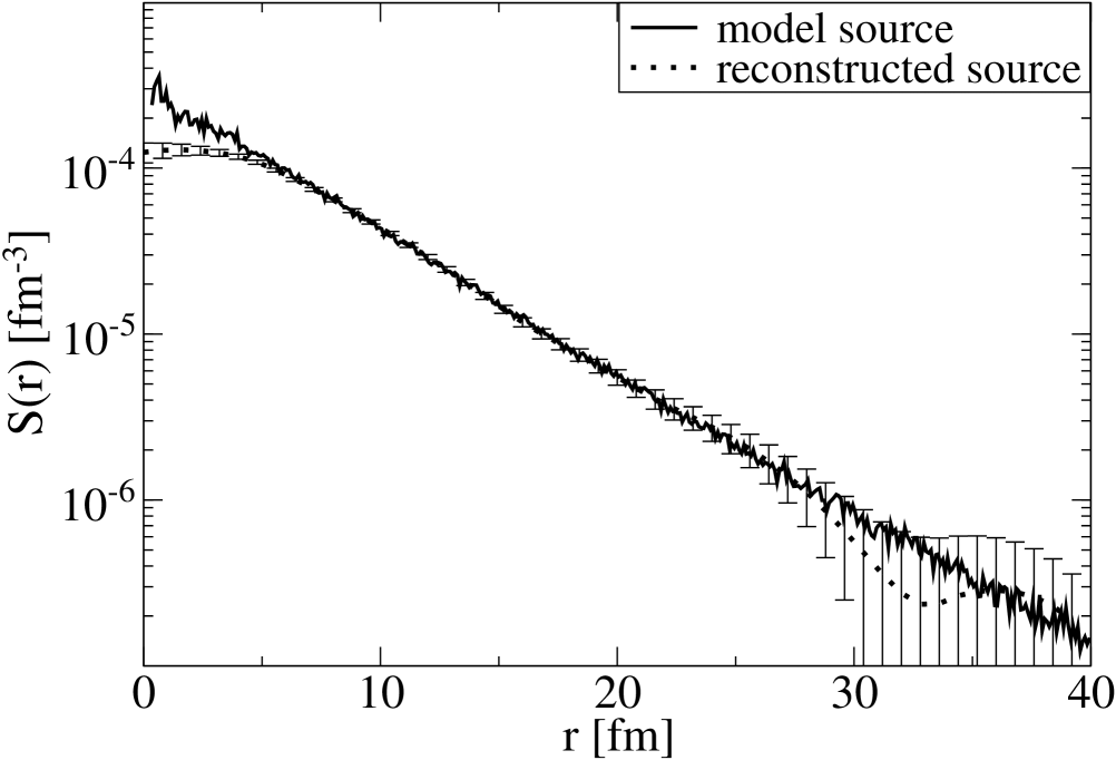
Figure 1: Comparison between the model source (solid curve) and the reconstructed source (dotted curve) with the AMPT model in the CMFP.

The imaging technique can be generalized as follows DAB97 ; DAB01 . Ignoring the interactions between the pions, the two-pion correlation function can be represented as UAW99

$$C({\bf q})=1+\int d^{4}{x}\cos({\bf q}\cdot{\bf r}-{\bigtriangleup E}{\bigtriangleup t})d(x),$$ (1)

where $d(x)$ is the so-called relative distance distribution. If we write this equation in the CMFP, the value of ${\bigtriangleup E}{\bigtriangleup t}$ is zero. Then, Eq. (1) can be written as

$$C({\bf q})=1+\int\cos({\bf q}{\cdot}{\bf r})S({\bf r})d{\bf r}.$$ (2)

Here $S({\bf r})=\int d(x)dt$ is the source function which describes the distribution of the relative separation of emission points for two particles. The angle-averaged version of Eq. (2) is

$$\mathcal{R}({q}) = C({q})-1=4\pi\int\frac{1}{{q}}{\sin({q}r)}{r}S(r)dr.$$ (3)

Finally, the one-dimensional source function $S(r)$ can be calculated by Fourier transform

$$S(r)=\frac{1}{2\pi^{2}}\frac{1}{r}\int\mathcal{R}({q}){q}\sin({q}{r})d{q}.$$ (4)

From above equations, we can see that the imaging technique is a model-independent way to obtain the source function in CMFP. The way of testing the validity of imaging technique is comparing the reconstructed source with the model sourceDAB01 ; DAB05 . The reconstructed source is the $S(r)$ calculated by imaging technique. The model source is gained by computing pairs of pions generated from the source with relative momentum less than $60$ MeV/$c$ DAB05 ; PAN99 . Now we take the String Melting AMPT(A Multi-Phase Transport) modelZWL05 for example, the source function of which has been analyzed by two-pion correlation functionsZWL09 ; Shan09 . We simulate Au+Au collisions source for the $\sqrt{s_{{}_{NN}}}=200$ GeV with $b=0$ fm, the number of events is 200. From Fig. 1 we can give corresponding result: the solid curve is computed by all the $\pi^{+}$ pairs which relative momentum is less than $60$ MeV/$c$ (similarly hereinafter); the dotted curve is calculated from correlation function with imaging technique. We can see that two curves are in good agreement, which means the imaging technique can work well in CMFP. The above is the brief summary of current one-dimensional imaging technique.

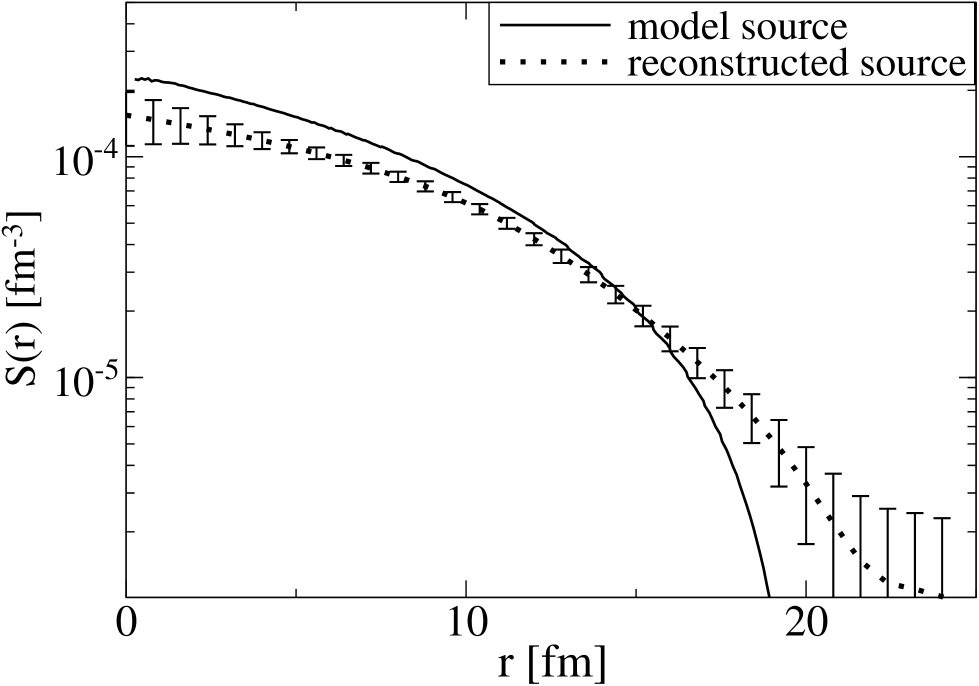
Figure 2: Comparison between the model source (solid curve) and the reconstructed source (dotted curve) with a homogeneous spherical model in the CMFS.

However, the CMFP is not a fixed frame, since different pair of pions has different center of mass velocity. In this paper, we try to improve this technique and intend to extract the source function $S(r)$ in the CMPS. To achieve this point, it is natural for us to use the Eq. (1)-(4) in the CMFS. We take the simple homogeneous spherical pion-emitting source with radius $r=10$ fm as the preliminary analysis object and set the momentum for the Boltzmann distribution ($T_{f}=158$ MeV). The purpose of setting such a simple source is not to conform experimental data, but convenient for us to analyze. In particular, we set the duration of particle emission time also in Gaussian distribution

$$f(t)=\left\{\begin{array}[]{l}\sqrt{{2}/{\pi}}\exp\left(-{t^{2}}/{2\tau^{2}}\right)/\tau~{}~{}~{}~{}~{}~{}~{}~{}~{}~{}~{}t>0,\\ \\ ~{}~{}~{}~{}~{}~{}~{}~{}~{}~{}~{}~{}0~{}~{}~{}~{}~{}~{}~{}~{}~{}~{}~{}~{}~{}~{}~{}~{}~{}~{}~{}~{}\hskip 10.243pt~{}~{}~{}~{}~{}t<0.\end{array}\right.$$ (8)

We set the standard deviation with $\tau=10$ fm/$c$ (similarly hereinafter). In Fig. 2, we compare the model source (solid curve) with the reconstructed source (dotted curve). Here the model source is gained by computing $10^{7}$ pairs of pions generated from the source. It can be seen that there exists obvious deviation. The reason is obvious: although the Eq. (1) can be written in any frame, $\triangle E\triangle t$ is not zero in the CMFS, which make the Eq. (2) inaccurate. To solve this problem, we intend to cut the pion pairs according to the difference of their energy and use the remaining pion pairs to build the correlation functions in CMFS. The reasons are as follows: For one thing, the Eq. (2) is close to accurate when the difference of energy tends to zero. For another, the energy of particle can be observed in laboratory. So this method can be used to analyse the experimental data.

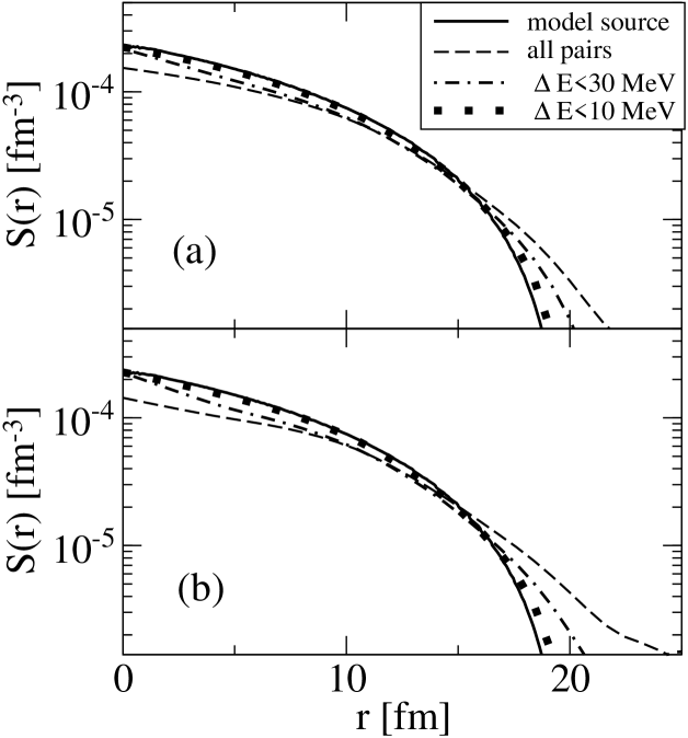
Figure 3: Correction of imaging results in the CMFS by cutting pairs according to their energy difference. In Fig. 3(a) we use the same model as in Fig. 2, while in Fig. 3(b) the momentum distribution is changed to a uniform form with $0$ to $1$ GeV/$c$.

In Fig. 3, we plot the reconstructed sources in the CMFS with the cuts of the energy difference of pion pair ($\triangle E$) less than $30$ MeV and $10$ MeV. (The dashed curve, dash-dotted curve and dotted curve are all imaging results. Due to the large number of curves, their error bars are not given in this figure.) From this figure, it can be seen that the difference between the imaging result and the real model source becomes smaller and smaller as the $\triangle E$ reduce. And we also find that when $\triangle E$ is set within $10$ MeV, this difference can almost be ignored, because $\triangle E\triangle t$ is very small in this situation. In Fig. 3 (b) we set the momentum to uniform distribution and get the corresponding result. We can see this method of $\triangle E$ cut is little influenced by momentum spectrum.

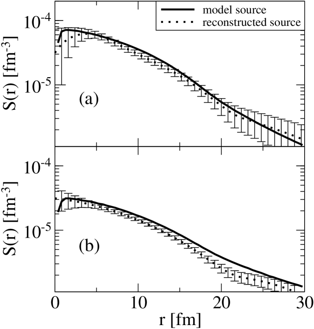
Figure 4: The same result of Fig. 3 but in the CMFP. The momentum is set for Boltzmann distribution (a) and uniform distribution from $0$ to $1$ GeV/$c$ (b).

For further discussing the feature of source function in the CMFS, in Fig. 4 we give the corresponding results of Fig. 3 but in the CMFP. Comparing with these results, we find two features claim out attention. First, in Fig. 3(a) and (b), we can see that the model source functions (solid curves) are almost exactly the same. While in Fig. 4(a) and (b), the model source functions (solid curves) exist obvious difference with different distribution of momentum. We think the reason is that they have the same source functions in a fixed frame. But this source function must be changed in the CMFP for the Lorentz transform. Obviously, the velocity of every pion pair must be influenced by the distribution of momentum. And then the source function will be influenced by the distribution of momentum in the CMFP. But the source function in the CMPS only depend on the scale of the particle emitting source and is little influenced by the distribution of momentum. Second, in the CMFS there does not exist the pairs of particles which distance is more than the diameter of the source obviously. This character can be seen in Fig. 3(a) and (b) where the radius is set to $10$ fm. But in Fig. 4(a) and (b) the source functions does not reduce to zero at the distance even more than $25$ fm. This means the source function in the CMFS can reflect the scale of the particle emitting source more directly.

3 Testing the imaging results in the CMFS

Figure 5: The model source function $S(r)$ obtained from the AMPT model with $b=0$ fm in the CMFS.

However, the problem is not the end. In our approach, the $\triangle t$ is gotten by counting the freeze out time in the CMFS. Of course, the $\triangle t$ is not zero and cannot be counted by experimental data. For removing the influence of $\triangle t$, we have to use the pion pairs with very small $\triangle E$ to build the correlation functions. More specifically, our investigation can only reconstruct the $S(r)$ of these pairs. Although this cut of pion pairs is according to the energy, it will influence the distribution of $S(r)$ more or less. Therefore, we must check the effect of this scheme with more realistic event generators. In Fig. 5 we give the model source functions with AMPT model. The situation is just the same as Fig. 1 but in the CMFS. The solid curve is the true model source. The dotted curve is also the model source which only computed by the $\pi^{+}$ pairs with $\bigtriangleup E<10$ MeV. It can be seen that the influence of $\bigtriangleup E$ cut on $S(r)$ is very small. In Fig. 6, we compare the model source and the reconstructed source (also with $\bigtriangleup E<10$ MeV) with different impact parameters. The number of events is 200 ($b=0$ fm), 500 ($b=5$ fm) and 10000 ($b=10$ fm), respectively. It can be seen that the two curves are in good agreement, except for the disagreement between the two curves in Fig.6(a) around $r=30$ fm. The actually obtained correlation function is discrete but not continuous, which is the reason for this disagreementDAB01 . We also tried to get the reconstructed source with smaller $\bigtriangleup E$, the result of which is the same as Fig. 6. This means $\bigtriangleup E<10$ MeV is small enough for giving the correct imaging results.

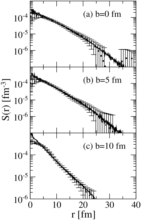
Figure 6: The comparison between the model source (solid curve) and the reconstructed source (dotted curve) in the CMFS. We set impact parameter (a) $b=0$ fm, (b) $b=5$ fm and (c) $b=10$ fm.

4 Summary

In this paper, we try to improve the imaging method for reconstructing the source function in the CMFS and obtain the following conclusions: Firstly, the source function in the CMFS can reflect the scale of the particle emitting source more directly than the CMFP. Secondly, we give a method to obtain the source function in the CMFS by cutting the pairs according to the difference of their energy which can be observed in laboratory. Using various models to test this method, we find when the energy difference $\bigtriangleup E<10$ MeV, the reconstructed source is a good approximation to the true model source. Finally, it is still a preliminary method which ignores interactions between the pions and is limited to one-dimensional problem at present. It means this method can only deal with the correlation function which is constructed by the Coulomb corrected experimental data. Further investigation of analysis and verification the possibility of getting more abundant and reliable information in the CMFS will also be of interest.

References

- (1) U. A. Wiedemann, U. Heinz, Phys. Rept. 319, 145 (1999).
- (2) R. M. Weiner, Phys. Rept. 327, 249 (2000).
- (3) M. A. Lisa, S. Pratt, R. Soltz, U. Wiedemann, Ann. Rev. Nucl. Part. Sci. 55, 357 (2005).
- (4) S. Chapman, P. Scotto, U. Heinz. Phys. Rev. Lett. 74, 4400 (1995).
- (5) S. Pratt. Nucl. Phys. A638, 125 (1998).
- (6) U. Heinz, B. V. Jacak, Ann. Rev. Nucl. Part. Sci. 49, 529 (1999).
- (7) D. A. Brown, P. Danielewicz, Phys. Lett. B 398, 252 (1997).
- (8) D. A. Brown, P. Danielewicz, Phys. Rev. C 57, 2474 (1998).
- (9) D. A. Brown, P. Danielewicz, Phys. Rev. C 64, 014902 (2001).
- (10) S. S. Adler et al., (PHENIX Collaboration), Phys. Rev. Lett. 98, 132301 (2007).
- (11) P. Chung, A. Taranenko, R. Lacey, W. Holzmann, J. Alexander, M. Issah, Nucl. Phys. A 749, 275 (2005).
- (12) P. Chung and P. Danielewicz (for the NA49 Collaboration), J. Phys. G 34, 1109 (2007).
- (13) P. Chung (for the PHENIX Collaboration), J. Phys. G 35, 044034 (2008).
- (14) S. Afanasiev et al., (PHENIX Collaboration), Phys. Rev. Lett. 100, 232301 (2008).
- (15) R. A. Lacey (for the PHENIX Collaboration), J. Phys. G 35, 104139 (2008).
- (16) Z. T. Yang, W. N. Zhang, L. Huo, J. B. Zhang, J. Phys. G 36, 015113 (2009).
- (17) Z. W. Lin, C. M. Ko, S. Pal, Phys. Rev. Lett. 89, 152301 (2002).
- (18) Z. W. Lin, C. M. Ko, J. Phys. G 30, 263 (2004).
- (19) T. Csögrő, S. Hegyi, W. A. Zajc, Eur. Phys. J. C 36, 67 (2004).
- (20) W. N. Zhang, Y. Y. Ren, C. Y. Wong, Phys. Rev. C 74, 024908 (2006).
- (21) Y. Y. Ren, W. N. Zhang, J. L. Liu, Phys. Lett. B 669, 317 (2008).
- (22) S. Nickerson, T. Csörgő, D. Kiang, Phys. Rev. C 57, 3251 (1998).
- (23) D. Hardtke, S. A. Voloshin, Phys. Rev. C 61, 024905 (2000).
- (24) E. Frodermann, U. Heinz, M. A. Lisa, Phys. Rev. C 73, 044908 (2006).
- (25) S. Y. Panitkin et al., (E895 Collaboration), Phys. Rev. Lett. 87, 112304 (2001).
- (26) G. Verde, D. A. Brown, P. Danielewicz, C. K. Gelbke, W. G. Lynch, M. B. Tsang, Phys. Rev. C 65, 054609 (2002).
- (27) P. Chung et al., (E895 Collaboration), Phys. Rev. Lett. 91, 162301 (2003).
- (28) P. Danielewicz, D. A. Brown, M. Heffner, S. Pratt, R. Soltz, Acta Phys. Hung. A 22, 253 (2005).
- (29) D. A. Brown, A. Enokizono, M. Heffner, R. Soltz, P. Danielewicz, S. Pratt, Phys. Rev. C 72, 054902 (2005).
- (30) P. Danielewicz, S. Pratt, Phys. Lett. B 618, 60 (2005).
- (31) P. Danielewicz, S. Pratt, Phys. Rev. C 75, 034907 (2007).
- (32) W. N. Zhang, Z. T. Yang, Y. Y. Ren, Phys. Rev. C 80, 044908 (2009).
- (33) S. Y. Panitkin, D. A. Brown, Phys. Rev. C 61, 021901 (1999).
- (34) Z. W. Lin, C. M. Ko, B. A. Li, B. Zhang, S. Pal, Phys. Rev. C 72, 064901 (2005).
- (35) Z. W. Lin, J. Phys. G 35, 104138 (2008).
- (36) L. Q. Shan, F. J. Wu, J. L. Liu, Q. C. Feng, Q. S. Wang, J. B. Zhang, L. Huo, J. Phys. G 36, 115102 (2009).