MAP inference via Block-Coordinate Frank-Wolfe Algorithm

Abstract

We present a new proximal bundle method for Maximum-A-Posteriori (MAP) inference in structured energy minimization problems. The method optimizes a Lagrangean relaxation of the original energy minimization problem using a multi plane block-coordinate Frank-Wolfe method that takes advantage of the specific structure of the Lagrangean decomposition. We show empirically that our method outperforms state-of-the-art Lagrangean decomposition based algorithms on some challenging Markov Random Field, multi-label discrete tomography and graph matching problems.

1 Introduction

Maximum-A-Posteriori (MAP) inference, that is minimizing an energy function $f:\mathcal{X}\rightarrow\mathbb{R}$ over a discrete set of labelings $\mathcal{X}$ is a central tool in computer vision and machine learning. Many solvers have been proposed for various special forms of energy $f$ and labeling space $\mathcal{X}$, see [11] for an overview of solvers and applications for the prominent special case of Markov Random Fields (MRF). Solvers can roughly be categorized into three categories: (i) Exact solvers that use search techniques (e.g. branch-and-bound) and possibly rely on solving lower bounds with LP-solvers to speed up search, (ii) primal heuristics that find a suboptimal solution with an ad-hoc search strategy adapted to the specific problem and (iii) Lagrangean decomposition (a.k.a. dual decomposition) based algorithms that decompose the original problem into smaller efficiently optimizable subproblems and exchange Lagrangean multipliers between subproblems until consensus between subproblems is achieved.

Except when the energy fulfills special assumptions, exact solvers are usually not applicable, since problem sizes in computer vision are too large. On the other hand, primal heuristics can be fast but solution quality need not be good and no information is given to judge it. Moreover, algorithms from the first two paradigms are usually developed ad-hoc for specific optimization problems and cannot be easily extended to other ones. Lagrangean decomposition based algorithms are a good middle ground, since they optimize a dual lower bound, hence can output a gap that shows the distance to optimum, yet use techniques that scale to large problem sizes. Generalization to new problems is also usually much easier, since subproblems can be readily combined.

A large number of algorithmic techniques have been proposed for optimizing a Lagrangean decomposition for MRFs, including (i) Message passing [16, 41, 37, 6] (a.k.a. block coordinate ascent, belief propagation), (ii) first order proximal splitting methods [26, 31] and (iii) Smoothing based methods [9, 29], (iv) Nesterov schemes [28, 10], (v) mirror descent [22], (vi) subgradient based algorithms [30, 36, 18]. In the case of MAP inference in MRFs, the study [11] has shown that message passing techniques outperform competing Lagrangean decomposition based methods by a large margin. However, there are two main practical shortcomings of message passing algorithms: (i) they need not converge to the optimum of the relaxation corresponding to the Lagrangean decomposition: while well-designed algorithms monotonically improve a dual lower bound, they may get stuck in suboptimal fixed points. (ii) So called min-marginals must be computable fast for all the subproblems in the given Lagrangean decomposition. While the above problems do not seem to be an issue for most MAP inference tasks in MRFs, for other problems they are. In such cases, alternative techniques must be used. Subgradient based methods can help here, since they do not possess the above shortcomings: They converge to the optimum of the Lagrangean relaxation and only require finding solutions to the subproblems of the decomposition, which is easier than their min-marginals (as needed for (i)), proximal steps (as needed for (ii)) or smoothed solutions (as needed for (iii) and (iv)).

The simplest subgradient based algorithm is subgradient ascent. However, its convergence is typically slow. Bundle methods, which store a series of subgradients to build a local approximation of the function to be optimized, empirically converge faster.

1.1 Contribution & Organization

We propose a multi plane block-coordinate version of the Frank-Wolfe method to find minimizing directions in a proximal bundle framework, see Section 2. Our method exploits the structure of the problem’s Lagrangean decomposition and is inspired by [34]. Applications of our approach to MRFs, discrete tomography and graph matching are presented in Section 3. An experimental evaluation on these problems is given in Section 4 and suggests that our method is superior to comparable established methods.

All proofs are given in the Appendix A. A C++-implementation of our Frank-Wolfe method is available at http://pub.ist.ac.at/~vnk/papers/FWMAP.html. The MRF, discrete tomography and graph matching solvers built on top of our method can be obtained at https://github.com/LPMP/LPMP.

1.2 Related work

To our knowledge, the Frank-Wolfe method has not yet been used in our general setting, i.e. underlying a proximal bundle solver for a general class of structured energy minimization problems. Hence, we subdivide related work into (i) subgradient/bundle methods for energy minimization, (ii) ad-hoc approaches that use Frank-Wolfe for specific tasks and (iii) proximal bundle methods.

Subgradient based solvers   have first been proposed by [36] for MAP-inference in MRFs and were later popularized by [18]. These works rely on a decomposition of MRFs into trees. New decompositions for certain MRFs were introduced and optimized in [25] for max-flow subproblems and in [32] for perfect matching subproblems. The work [43] used a covering of the graph by a tree and optimized additional equality constraints on duplicated nodes via subgradient ascent. Usage of bundle methods that store a series of subgradients to build a local approximation of the objective function was proposed by [12, 32] for MAP inference in MRFs.

The Frank-Wolfe   algorithm was developed in the 50s [4] and was popularized recently by [8]. In [20] a block coordinate version of Frank-Wolfe was proposed and applied to training structural SVMs. Further improvements were given in [34, 24] where, among other things, caching of planes was proposed for the Frank-Wolfe method. Several works have applied Frank-Wolfe to the MAP-MRF inference problem: (1) [33] used Frank-Wolfe to compute an approximated steepest-descent direction in the local polytope relaxation for MRFs. (2) [23] used Frank-Wolfe to solve a modified problem obtained by adding a strictly convex quadratic function to the original objective (either primal or dual). In contrast to these works, we use Frank-Wolfe inside a proximal method. Furthermore, the papers above use a fine decomposition into many small subproblems (corresponding to pairwise terms of the energy function), while we decompose the problem into much larger subproblems. In general, our decomposition results in fewer dual variables to optimize over, and each Frank-Wolfe update can be expected to give a much larger gain. Frank-Wolfe was also used in [1] for MAP inference in dense MRFs with Potts interactions and Gaussian weights. As we do, they use Frank-Wolfe to optimize proximal steps for MAP-inference. In constrast to our work, they do not optimize Lagrangean multipliers, but the original variables directly. In other words, they work in the primal, while we work in the dual. We remark that our formulation is applicable to more general integer optimization problems than either [33, 23, 1] and it does not seem straightforward to apply these approaches to our more general setting while only requiring access to MAP-oracles of subproblems.

Proximal bundle methods   were introduced in [13, 21] to accelerate subgradient descent algorithms. They work by locally building an approximation (bundle) to the function to be optimized and use this bundle to find a descent direction. For stability, a quadratic (proximal) term is added [14]. While not theoretically guaranteed, proximal bundle methods are often faster than subgradient methods.

2 Method

Original problem   We consider the problem of minimizing a function of Boolean variables represented as a sum of individual terms:

$$\min_{x\in\{0,1\}^{d}}f(x),\quad f(x):=\sum_{t\in T}f_{t}(x_{A_{t}})$$ (1)

Here term $t\in T$ is specified by a subset of variables $A_{t}\subseteq[d]$ and a function $f_{t}:\{0,1\}^{A_{t}}\rightarrow\mathbb{R}\cup\{+\infty\}$ of $|A_{t}|$ variables. Vector $x_{A_{t}}\in\mathbb{R}^{A_{t}}$ is the restriction of vector $x\in\mathbb{R}^{d}$ to $A_{t}$. The arity $|A_{t}|$ of function $f_{t}$ can be arbitrarily large, however we assume the existence of an efficient min-oracle that for a given vector $\lambda\in\mathbb{R}^{A_{t}}$ computes $x\in\operatorname*{arg\,min}\limits_{x\in\operatorname*{dom}f_{t}}\left[f_{t}(x)+\langle\lambda,x\rangle\right]$ together with the cost $f_{t}(x)$, where $\operatorname*{dom}f_{t}=\{x\in\{0,1\}^{A_{t}}\>|\>f_{t}(x)<+\infty\}\neq\varnothing$ is the effective domain of $f_{t}$. It will be convenient to denote

$$h_{t}(\lambda)\!=\!\!\!\!\!\min\limits_{\stackrel{{\scriptstyle}}{{x\in\operatorname*{dom}f_{t}}}}\!\!\!\!\!\left[f_{t}(x)+\langle\lambda,x\rangle\right]\!=\!\min\limits_{y\in\mathcal{Y}_{t}}\langle y,[\lambda\;1]\rangle\!=\!\min\limits_{y\in\mathbb{Y}_{t}}\langle y,[\lambda\;1]\rangle$$

where subsets $\mathcal{Y}_{t},\mathbb{Y}_{t}\subseteq[0,1]^{A_{t}}\otimes\mathbb{R}$ are defined as follows:

$$\mathcal{Y}_{t}=\{[x\;f_{t}(x)]\>:\>x\in\operatorname*{dom}f_{t}\}\;\quad\mathbb{Y}_{t}=\operatorname{conv}(\mathcal{Y}_{t})$$

The assumption means that we can efficiently compute a supergradient of concave function $h_{t}(\lambda)$ at a given $\lambda\in\mathbb{R}^{A_{t}}$.

Since (1) is in general an NP-hard problem, our goal will be to solve a certain convex relaxation of (1), which will turn out to be equivalent to the Basic LP relaxation (BLP) of (1) [17]. This relaxation has been widely studied in the literature, especially for the MAP-MRF problem (in which case it is usually called the local polytope relaxation [40, 41]). We emphasize, however, that our methodology is different from most previous works: before applying the BLP relaxation, we represent the objective as a function of Boolean indicator variables. This allows expressing complicated combinatorial constraints such as those in multi-label discrete tomography and graph matching problems (see Section 3).

Lagrangean relaxation   For a vector $y\in\mathbb{Y}_{t}$ let us denote the first $|A_{t}|$ components as $y_{\star}\in[0,1]^{A_{t}}$ and the last one as $y_{\circ}\in\mathbb{R}$ (so that $y=[y_{\star}\;y_{\circ}]$). We also denote $\mathcal{Y}=\bigotimes_{t\in T}\mathcal{Y}_{t}$ and $\mathbb{Y}=\bigotimes_{t\in T}\mathbb{Y}_{t}=\operatorname{conv}(\mathcal{Y})$. The $t$-th component of vector $y\in\mathbb{Y}$ will be denoted as $y^{t}\in\mathbb{Y}_{t}$. Problem (1) can now be equivalently written as

$$\min_{\begin{subarray}{c}y\in\mathbb{Y}\;,\;x\in\{0,1\}^{d}\\ y^{t}_{\star}=x_{A_{t}}\;\forall t\in T\end{subarray}}\;\;\sum_{t\in T}y^{t}_{\circ}$$ (2)

We form the relaxation of (2) by removing the non-convex constraint $x\in\{0,1\}^{d}$:

$$\min_{\begin{subarray}{c}y\in\mathbb{Y}\;,\;x\in\mathbb{R}^{d}\\ y^{t}_{\star}=x_{A_{t}}\;\forall t\in T\end{subarray}}\;\;\sum_{t\in T}y^{t}_{\circ}$$ (3)

It can be shown that problem (3) is equivalent to the BLP relaxation of (1), see [swoboda:2018arxiv].

We will not directly optimize this relaxation, but its Lagrangean dual [35]. For each equality constraint $y^{t}_{\star}=x_{A_{t}}$ we introduce Lagrange multipliers $\lambda^{t}\in\mathbb{R}^{A_{t}}$. The collection of these multipliers will be denoted as $\lambda\in\bigotimes_{t\in T}\mathbb{R}^{A_{t}}$. The dual will be optimized over the set

$$\Lambda=\left\{\lambda\>:\>\sum\limits_{t\in T_{i}}\lambda^{t}_{i}=0\;\;\;\forall i\in[d]\right\}$$ (4)

where we denoted

$$T_{i}=\{t\in T\>:\>i\in A_{t}\}\,.$$

Proposition 1.

The dual of (3) w.r.t. the equality constraints $y^{t}_{\star}=x_{A_{t}}$ is

$$\max_{\lambda\in\Lambda}h(\lambda),\quad h(\lambda):=\sum_{t\in T}h_{t}(\lambda^{t})$$ (5)

Furthermore, the optimal values of problems (3) and (5) coincide. (This value can be $+\infty$, meaning that (3) is infeasible and (5) is unbounded).

Next, we describe how we maximize function $h(\lambda)$.

Proximal term   We have a non-smooth concave maximization problem in $\lambda$, hence algorithms that require a differentiable objective functions will not work. In proximal bundle methods [14] an additional proximal term is added. This results in the new objective

$$\max_{\lambda\in\Lambda}h_{\mu,c}(\lambda),\quad h_{\mu,c}(\lambda):=h(\lambda)-\frac{1}{2c}\lVert\lambda-\mu\rVert^{2}$$ (6)

for a center point $\mu\in\Lambda$. The proximal quadratic terms act as a trust-region term in the vicinity of $\mu$ and make the function strongly concave, hence smoothing the dual. A successively refined polyhedral approximation [21] is typically used for solving (6). We develop a proximal method that will alternate between minimizing (6) with the help of a multi-plane block coordinate Frank-Wolfe method and updating the proximal center $\mu$.

2.1 Maximizing $h_{\mu,c}(\lambda)$: BCFW algorithm

Objectives similar to (6) (without the summation constraint on the $\lambda$-variables) are used for training structural Support Vector Machines (SSVMs). Following [20, 34, 24], we use a block-coordinate Frank-Wolfe algorithm (BCFW) applied to the dual of (6), more specifically its multi-plane version MP-BCFW [34]. The dual of (6) is formulated below.

Proposition 2.

The dual problem to $\max_{\lambda\in\Lambda}h_{\mu,c}(\lambda)$ is

$$\min\limits_{y\in\mathbb{Y}}f_{\mu,c}(y),\\ f_{\mu,c}(y):=\max\limits_{\lambda\in\Lambda}\sum_{t\in T}\left[\langle y^{t},[\lambda^{t}\;1]\rangle-\frac{1}{2c}\lVert\lambda^{t}-\mu^{t}\rVert^{2}\right]$$ (7)

Define $\nu\in\mathbb{R}^{d}$ by $\nu_{i}=\frac{1}{|T_{i}|}\sum_{t\in T_{i}}(c\cdot y^{t}_{i}+\mu^{t}_{i})$ for $i\in[d]$. Then the optimal $\lambda$ in (7) is $\lambda^{t}=c\cdot y^{t}_{\star}+\mu^{t}-\nu_{A_{t}}$ and

$$f_{\mu,c}(y) = \sum_{t\in T}\left(\frac{c}{2}\lVert y^{t}_{\star}\rVert^{2}+\langle y^{t},[\mu^{t}\;1]\rangle\right)-\sum_{i=1}^{d}\frac{|T_{i}|}{2c}\nu_{i}^{2}$$

$$\nabla_{t}f_{\mu,c}(y) = [\lambda^{t}\;1]$$ (8)

where $\nabla_{t}$ denotes the derivative w.r.t. variables $y^{t}$.

Next, we review and adapt to our setting BCFW and MP-BCFW algorithms for minimizing function $f_{\mu,c}(y)$ over $y\in\mathbb{Y}$. We will also describe a practical improvement to the implementation, namely compact representation of planes, and discuss the problem of estimating the duality gap.

BCFW [20]   The algorithm maintains feasible vectors $y\in\mathbb{Y}$. At each step BCFW tries to decrease the objective $f_{\mu,c}(y)$ by updating component $y^{t}$ for a chosen term $t$ (while maintaining feasibility). To achieve this, it first linearizes the objective by using the Taylor expansion around the current point:

$$f_{\mu,c}(z)\approx\langle\nabla f_{\mu,c}(y),z\rangle+{\tt const}\,.$$ (9)

The optimal solution $z^{t}\in\mathbb{Y}_{t}$ of the linearized objective is computed by calling the $t$-th oracle: $z^{t}\leftarrow\operatorname*{arg\,min}\limits_{z^{t}\in\mathcal{Y}_{t}}\langle\nabla_{t}f_{\mu,c}(y),z^{t}\rangle$. The new vector $y$ is obtained as the best interpolation of $y^{t}$ and $z^{t}$ with all other components $s\neq t$ fixed to $y^{s}$, i.e. $y^{s}(\gamma)\leftarrow\left\{\begin{array}[]{ll}y^{s},&s\neq t\\ (1-\gamma)y^{t}+\gamma z^{t},&s=t\end{array}\right.$. The step size $\gamma\in[0,1]$ is chosen to minimize the objective. The optimal $\gamma$ can be easily computed in closed form (see Lemma 1 in [swoboda:2018arxiv]). One pass of BCFW is summarized in Algorithm 1. To avoid the expensive recomputation of the sum $\nu$ in Prop. 2 needed for computing the gradient and the step size, it is held and updated explicitly in Algorithm 1.

Algorithm 1 One pass of BCFW. Input: vectors $y\in\mathbb{Y}$, $\mu\in\Lambda$ and $\nu\in\mathbb{R}^{d}$ computed as in Prop. 2.

1:  for each $t\in T$ do in a random order

2:    set $\lambda^{t}=c\cdot y^{t}_{\star}+\mu^{t}-\nu_{A_{t}}$

3:    call $t$-th oracle for $\lambda^{t}$:   $z^{t}\leftarrow\operatorname*{arg\,min}\limits_{z^{t}\in\mathcal{Y}_{t}}\langle z^{t},[\lambda^{t}\;1]\rangle$    (i.e. let $x\leftarrow\operatorname*{arg\,min}\limits_{x\in\mathcal{X}_{t}}[f_{t}(x)+\langle\lambda^{t},x\rangle]$ and $z^{t}=[x\;f_{t}(x)]$)

4:    interpolate $y(\gamma)^{s}\leftarrow\left\{\begin{array}[]{ll}y^{s},&s\neq t\\ (1-\gamma)y^{t}+\gamma z^{t},&s=t\end{array}\right.$

5:    compute $\gamma\leftarrow\operatorname*{arg\,min}_{\gamma\in[0,1]}f_{\mu,c}(y(\gamma))$:   set $\gamma\leftarrow\frac{\langle[\lambda^{t}\;1],z^{t}-y^{t}\rangle}{c\lVert y^{t}_{\star}-z^{t}_{\star}\rVert^{2}}$ and clip $\gamma$ to $[0,1]$

6:    set $\nu_{i}\leftarrow\nu_{i}+\frac{c}{|T_{i}|}(y(\gamma)^{t}_{i}-y^{t}_{i})$ for $i\in A_{t}$ and $y^{t}\leftarrow y(\gamma)^{t}$ ​​​​

7:  end for

MP-BCFW [34]   In this paper we use the multi-plane version of BCFW. This method caches planes $z^{t}$ returned by min-oracles for terms $h_{t}(\lambda^{t})=\min_{z^{t}\in\mathcal{Y}_{t}}\langle z^{t},[\lambda^{t}\ 1]\rangle$. Let $\tilde{\mathcal{Y}}_{t}\subset\mathcal{Y}_{t}$ be the set of planes currently stored in memory for the $t$-th subproblem. It defines an approximation $\tilde{h}_{t}(\lambda^{t})=\min_{z^{t}\in\tilde{\mathcal{Y}}^{t}}\langle z^{t},[\lambda^{t}\ 1]\rangle$ of term $h_{t}(\lambda^{t})$. Note that $\tilde{h}_{t}(\lambda^{t})\geq h_{t}(\lambda^{t})$ for any $\lambda^{t}$.

MP-BCFW uses exact passes (that call the “exact” oracle for $h_{t}(\lambda^{t})$ in line 3 of Algorithm 1) and approximate passes (that call the “approximate” oracle for $\tilde{h}_{t}(\lambda^{t})$). One MP-BCFW iteration consists of one exact pass followed by several approximate passes. The number of approximate passes is determined automatically by monitoring how fast the objective decreases per unit of time. Namely, the method computes the ratio $\frac{f_{\mu,c}(y^{\circ})-f_{\mu,c}(y)}{\Delta t}$ where $y^{\circ}$ is the vector at the beginning of the MP-BCFW iteration, $y$ is the current vector and $\Delta t$ is the time passed since the beginning of the MP-BCFW iteration. If this ratio drops after an approximate pass then the iteration terminates, and a new MP-BCFW iteration is started with an exact pass. The number of approximate passes will thus depend on the relative speed of exact and approximate oracles.

Note that the time for an approximate oracle call is proportional to the size of the working set $|\tilde{\mathcal{Y}}_{t}|$. The method in [34] uses a common strategy for controlling this size: planes that are not used during the last $K$ iterations are removed from $\mathcal{Y}_{t}$. We use $K=10$, which is the default parameter in [34].

Compact representation of planes   Recall that planes in the set $\tilde{\mathcal{Y}}_{t}$ have the form $[x\;f_{t}(x)]$ for some $x\in\operatorname*{dom}f_{t}\subseteq\{0,1\}^{A_{t}}$. A naive approach (used, in particular, in previous works [34, 24]) is to store them explicitly as vectors of size $|A_{t}|+1$. We observe that in some applications a special structure of $\mathcal{X}_{t}$ allows storing and manipulating these planes more efficiently. For example, in MAP-MRF inference problems a variable with $k$ possible values can be represented by a single integer, rather than $k$ indicator variables.

In our implementation we assume that each vector $x\in\operatorname*{dom}f_{t}$ can be represented by an object $s$ in a possibly more compact space ${\mathbb{X}}_{t}$. To specify term $f_{t}$, the user must provide an array $\operatorname{map}_{t}:[|A_{t}|]\rightarrow[d]$ that determines set $A_{t}\subseteq[d]$ in a natural way, specify the size of objects $s\in{\mathbb{X}}_{t}$, and implement the following functions:

• A bijection $\sigma_{t}:{\mathbb{X}}_{t}\rightarrow\mathcal{X}_{t}$.

• Min-oracle that for a given $\lambda_{t}$ computes $x\in\operatorname*{arg\,min}\limits_{x\in\operatorname*{dom}f_{t}}[f_{t}(x)+\langle\lambda^{t},x\rangle]$ and returns its compact representation $s$ (i.e.  $\sigma_{t}(s)\!=\!x$) together with the cost $f_{t}(x)$.

• A function that computes inner product $\langle\lambda^{t},\sigma_{t}(s)\rangle$ for a given vector $\lambda^{t}$ and object $s\in{\mathbb{X}}_{t}$.

Note, calling the approximate oracle in line 3 involves calling the function in (F3) $|\tilde{\mathcal{Y}}_{t}|$ times; it typically takes $O(|\tilde{\mathcal{Y}}_{t}|\cdot{\tt size}_{t})$ time where ${\tt size}_{t}$ is the length of the array for storing $s\in{\mathbb{X}}_{t}$.

Remark 1.

The efficient plane storage mechanism gives roughly a $25\%$ speedup of a single MP-BCFW pass on the protein-folding MRF dataset (see Sections 3 and 4). Moreover, it typically results in a slightly better objective value obtained after each MP-BCFW pass, since more approximate passes can be done before an exact pass is called (since approximate passes are accelerated by the compact plane storage, their objective decrease per unit of time is higher, hence they are called more often).

2.2 Algorithm’s summary

Recall that our goal is to maximize function $h(\lambda)$ over $\lambda\in\Lambda$; this gives a lower bound on the original discrete optimization problem $\min_{x\in\mathcal{X}}f(x)$. We now summarize our algorithm for solving $\max_{\lambda\in\Lambda}h(\lambda)$, and describe our choices of parameters. To initialize, we set $\mu^{t}={\bf 0}$, $y^{t}\leftarrow\operatorname*{arg\,max}_{y^{t}\in\mathcal{Y}_{t}}\langle y^{t},[\mu^{t}\;1]\rangle$ and $\tilde{\mathcal{Y}}=\{y^{t}\}$ for each $t\in T$. Then we start the main algorithm. After every 10 iterations of MP-BCFW we update $\mu\leftarrow\lambda^{\ast}$ (keeping vectors $y^{t}$ and sets $\tilde{\mathcal{Y}}_{t}$ unchanged), where $\lambda^{\ast}$ is the vector with the largest value of objective $h(\lambda^{\ast})$ seen so far. Since evaluating $h(\lambda)$ is an expensive operation, we do it for the current vector $\lambda$ only after every 5 iterations of MP-BCFW.

Remark 2 (Convergence).

If we evaluated the inner iterations in MP-BCFW exactly, our method would amount to the proximal point algorithm which is convergent [27]. Even with non-exact evaluation, convergence can be proved when the error in the evaluation of the proximal is shrinking fast enough towards zero. However, we have use a more aggressive scheme that updates the proximal point every 10 iterations and does not bound the inexactness of the proximal step evaluation. Experimentally, we have found that it gives good results w.r.t. the objective of the overall problem (5).

2.3 Estimating duality gap

To get a good stopping criterion, it is desirable to have a bound on the gap $h(\lambda)-h(\lambda^{\ast})$ between the current and optimal objectives. This could be easily done if we had feasible primal and dual solutions. Unfortunately, in our case vector $y\in\mathbb{Y}$ is not a feasible solution of problem (3), since it does not satisfy equality constraints $y^{t}_{\star}=x_{A_{t}}$. To get a handle on the duality gap, we propose to use the following quantities:

$$A_{y,\lambda}\!=\!\sum_{t\in T}\langle y^{t},[\lambda^{t}\;1]\rangle-h(\lambda)\;,\;B_{y}\!=\!\sum_{i=1}^{d}\left[\max_{t\in T_{i}}y^{t}_{i}-\min_{t\in T_{i}}y^{t}_{i}\right]$$ (10)

Proposition 3.

Consider pair $(y,\lambda)\in\mathbb{Y}\!\times\!\Lambda$.
(a) There holds $A_{y,\lambda}\geq 0$, $B_{y}\geq 0$ and

$$h(\lambda^{\ast})-h(\lambda)\leq A_{y,\lambda}+B_{y}\cdot\lVert\lambda^{\ast}-\lambda\rVert_{1,\infty}\quad\forall\lambda^{\ast}\in\Lambda$$ (11)

where we denoted $\lVert\delta\rVert_{1,\infty}=\max_{i\in[d]}\sum_{t\in T_{i}}|\delta^{t}_{i}|$.
(b) We have $A_{y,\lambda}=B_{y}=0$ if and only if $y$ and $\lambda$ are optimal solutions of problems (3) and (5), respectively.

Note, if we knew that an optimal solution $\lambda^{\ast}\in\max_{\lambda\in\Lambda}h(\lambda)$ belongs to some bounded region then we could use (11) to obtain a bound on the duality gap. Such region can be obtained for some applications, but we did not pursue this direction.

3 Applications

In this section we give a detailed description of the three applications used in the evaluation: Markov Random Fields (MRFs), discrete tomography and the graph matching problem. The latter two are both extensions of the MAP-inference problems for MRFs. Those three problems are reviewed below.

3.1 Markov Random Fields

An MRF consists of a graph $G=(V,E)$ and a discrete set of labels $\mathcal{X}_{v}$ for each $v\in V$. The goal in Maximum-A-Posteriori (MAP) inference is to find labeling $(x_{v})_{v\in V}\in\bigotimes_{v\in V}\mathcal{X}_{v}=:\mathcal{X}$ that is minimal with respect to the potentials:

$$\min_{x\in\mathcal{X}}f(x),\;f(x):=\sum_{v\in V}\theta_{v}(x_{v})+\sum_{uv\in E}\theta_{uv}(x_{u},x_{v})\,.$$ (12)

This problem is NP-hard for general graphs $G$, but can be solved efficiently for trees. Hence, we choose a covering $G$ by trees, as done in [18]. Additionally, we seek a small number of trees, such that the number of Lagrangean variables stays small and optimization becomes faster.

Arboricity   A tree covering of a graph is called a minimal tree cover, if there is no covering consisting of fewer trees. The associated number of trees is called the graph’s arboricity. We compute the graph’s arboricity together with a minimal tree cover efficiently with the method [5]

Boolean encoding   To phrase the problem as an instance of (1), we encode labelings $x\in\mathcal{X}$ via indicator variables $x_{i;a}=[x_{i}=a]\in\{0,1\}$ for $i\in V,a\in\mathcal{X}_{i}$ while adding constraints $\sum_{a}x_{i;a}=1$ (i.e. assigning infinite cost to configurations that do not satisfy this constraint).

A tree cover and a Boolean encoding are also used for the two problems below; we will not explicitly comment on this anymore.

3.2 Discrete tomography

Figure 1: Illustration of a discrete tomography problem. Image intensity values are 0 (white), 1 (gray) and 2 (black). Small arrows on the side denote the three tomographic projection directions (horizontal, vertical, and diagonal). Values at arrow heads denote the intensity value along tomographic projections.

Figure 2: Illustration of a graph matching problem matching nose and left/right feet of two penguins. The blue nodes on the left penguin correspond to the underlying node set $V$, while the blue nodes on the right penguin correspond to the labels $\mathcal{L}$. The green lines denotes the matching. Note that no two labels are matched twice. The red springs denote pairwise costs $\theta_{ij}$ that encourage geometric rigidity of the matching.

The discrete tomography problem is to reconstruct an image from a set of linear (tomographic) projections taken at different angles, where image intensity values are restricted to be from a discrete set of intensities. See Figure 2 for an illustration. The problem is ill-posed, since the number of linear projections is smaller than the number of pixels to reconstruct. Hence, we use a regularizer to penalize non-regular image structures. Formally, we have an MRF $G=(V,E)$, where the node set corresponds to the pixel grid and the edges connect nodes which correspond to neighboring pixels. The label space is $\mathcal{X}_{v}=\{0,1,\ldots,k\}$ for some $k\in\mathbb{N}$. Additionally, the labeling $x\in\mathcal{X}$ must satisfy linear projections $Ax=b$ with $A\in\{0,1\}^{\lvert V\rvert\times l}$. Usually, no local information is available, hence the unary potentials are zero: $\theta_{v}\equiv 0$ for $v\in V$. The problem reads

$$\min_{x\in\mathcal{X}}f(x),\quad f(x):=\sum_{ij\in E}\theta_{ij}(x_{i},x_{j})$$ (13)

where $\mathcal{X}=\{x\in\{0,1,\ldots,k\}^{V}\>:\>Ax=b\}$. A typical choice for the pairwise potentials $\theta_{ij}$ is the truncated $L_{1}$-norm $\theta_{ij}(x_{i},x_{j})=\min(\lvert x_{i}-x_{j}\rvert,c)$. Each row of the projections $Ax=b$ forms another subproblem. The $i$-th row of $Ax=b$ hence is of the form $\sum_{v\in V:A_{iv}=1}x_{v}=b_{i}$. Efficient solvers for this problem were recently considered in [19]. We follow their recursive decomposition approach for the solution of the projection subproblems. Details are given below.

Discrete tomography subproblems

We use a simplified version of the recursive decomposition approach of [19] for efficiently solving the summation constraints $Ax=b$ of the discrete tomography problem. Below we give the corresponding details. Let the $i$-th row of $Ax=b$ be of the form $\sum_{v\in V:A_{iv}=1}x_{v}=b_{i}$ and recall that $x_{v}\in\{0,1,\ldots,k\}$. Each such tomographic projection will correspond to a single subproblem. Taking care of Lagrangean multipliers $\lambda$, we can rename variables and rewrite the problem as

$$\min_{x_{1},\ldots,x_{n}\in\{0,\ldots,k\}^{n}}\sum_{i=1}^{n}\sum_{l=0}^{k}\lambda_{i}(l)\cdot\mathbbmss{1}_{x_{i}=l}\quad\text{s.t.}\quad\sum_{i=1}^{n}x_{i}=b$$ (14)

We will follow a recursive decomposition approach. To this end, we introduce helper summation variables $s_{i:j}=\sum_{u=i}^{j}x_{u}$.

Variable partitions

We partition the set $[1,n]$ into $\Pi_{1:\lfloor\frac{n}{2}\rfloor}=\{x_{1},\ldots,x_{\lfloor\frac{n}{2}\rfloor}\}$ and $\Pi_{\lfloor\frac{n}{2}\rfloor+1:n}=\{x_{\lfloor\frac{n}{2}\rfloor+1},\ldots,x_{n}\}$. We recursively partition $\Pi_{1:\lfloor\frac{n}{2}\rfloor}$ and $\Pi_{\lfloor\frac{n}{2}\rfloor+1:n}$ analoguously until reaching single variables. This results in a tree with $\Pi_{1:n}$ as root.

Constraints on summation variables

Whenever we have partitions $\Pi_{i:j}=\Pi_{i:k}\cup\Pi_{k+1:j}$, we add the constraint $s_{i:j}=s_{j:k}+s_{k+1:j}$.

Solving (14)

We will propose a dynamic programming approach to solving (14). First, for each value $l$ of summation variable $s_{i:j}$ we store a value $\phi_{i:j}(l)\in\mathbb{R}$. We compute $\phi_{i:j}$ recursively from leaves to the root. For partitions $\Pi_{i:j}=\Pi_{i:k}\cup\Pi_{k+1:j}$ we compute

$$\phi_{i:j}(l)=\min_{l^{\prime}=0,\ldots,l}\phi_{i:k}(l^{\prime})+\phi_{k+1,j}(l-l^{\prime})\quad\forall l\,.$$ (15)

After having computed $\phi_{1:n}$, we set $s^{*}_{1:n}=b$. Subsequently, we make a pass from root to leaves to compute the optimal label sum for each variable $s_{i:j}$ as follows:

$$s^{*}_{i:k},s^{*}_{k+1:j}=\min_{s_{i:k}+s_{k+1:j}=s^{*}_{i:j}}\phi_{i:k}(s_{i:k})+\phi_{k+1:j}(s_{k+1:j})\,.$$ (16)

Fast dynamic programming

Naively computing (15) needs $O(((j-i)\cdot k)^{2})$ steps. However, we use an efficient heuristic [3] that tends to have subquadratic complexity in practice.

3.3 Graph matching

The graph matching problem consists of finding a MAP-solution in an MRF $G=(V,E)$ where the labels for each node come from a common universe $\mathcal{X}_{v}\subset\mathcal{L}$ $\forall v\in V$. The additional matching constraint requires that two nodes cannot take the same label: $x_{u}\neq x_{v}$ $\forall u,v\in V,u\neq v$. Hence, any feasible solution defines an injective mapping into the set of labels. For an illustration see Figure 2. The problem is

$$\min_{x\in\mathcal{X}}f(x)\quad\text{ s.t. }\quad x_{u}\neq x_{v}\quad\forall u\neq v\,.$$ (17)

We use a minimum cost flow solver for handling the matching constraint, see e.g. [39, 44, 38] for an explanation of the minimum cost flow solver construction.

4 Experiments

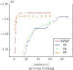
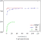
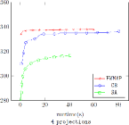
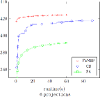
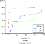
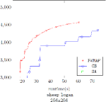
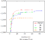
Figure 3: Averaged lower bound vs. runtime plots for the protein folding MRF dataset, discrete tomography (synthetic images with $2$, $4$ and $6$ projections, sheep logan image of sizes $64\times 64$ and $256\times 256$ with $2$, $4$ and $6$ projections), and the 6d scene flow graph matching dataset. Values are averaged over all instances of the dataset.

Dataset	# I	$\lvert V\rvert$	$\lvert E\rvert$	FWMAP	CB	SA	MP
MRF
protein folding	11	33-40	528-780	-12917.44	-12970.61	-12960.30	-13043.67
Discrete tomography
synthetic 2 proj.	9	1024	1984	266.12	265.89	239.39	$\dagger$
synthetic 4 proj.	9	1024	1984	337.88	336.33	316.61	$\dagger$
synthetic 6 proj.	9	1024	1984	424.36	417.76	391.09	$\dagger$
sheep logan $\mathbf{64\times 64}$	3	4096	8064	897.18	847.87	701.93	$\dagger$
sheep logan $\mathbf{256\times 256}$	3	65536	130560	4580.06	4359.24	370.63	$\dagger$
Graph matching
6d scene flow	6	48-126	1148-5352	-2864.2	-2865.61	-2867.60	-2877.08

Table 1: Dataset statistics and averaged maximum lower bound. # I denotes number of instances in dataset, $\lvert V\rvert$ the number of nodes and $\lvert E\rvert$ the number of edges in the underlying graphical model. $\dagger$ means method is not applicable. Bold numbers indicate highest lower bound among competing algorithms.

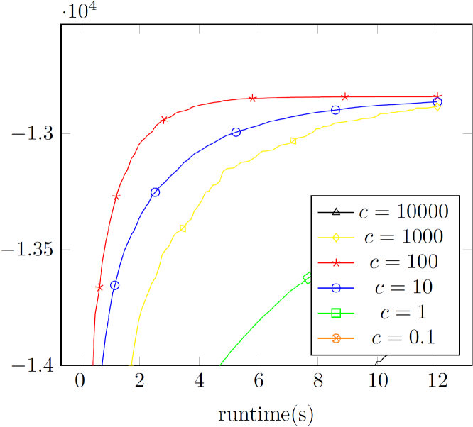
Figure 4: lower bound vs. runtime on instance 1CKK of the protein folding dataset solved with FWMAP and different values of proximal weight $c$ from (6).

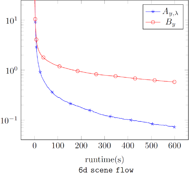
Figure 5: Duality gap quantities $A_{y,\lambda}$ and $B_{y}$ from (10) over time for the synthetic 6 proj. dataset from discrete tomography.

We have chosen a selection of challenging MRF, discrete tomography and graph matching problems where message passing methods struggle or are not applicable. Detailed descriptions of these problems can be found in Appendix A.

Remark 3.

Note that there are a large number of MRF and graph matching problems where message passing is the method of choice due to its greater speed and sufficient solution quality, see [11, 38]. In such cases there is no advantage in using subgradient based solvers, which tend to be slower. However, our chosen evaluation problems contain some of the most challenging MRF and graph matching problems with corresponding Lagrangean decompositions not solved satisfactorily with message passing solvers.

We have excluded primal heuristics that do not solve a relaxation corresponding to our Lagrangean decomposition at all from comparison. First, they do not deliver any lower bounds, hence cannot be directly compared. Second, we see them as complementary solvers, since, when they are applied on the solved dual problem, their solution quality typically improves. We have run every instance for 10 minutes on a Intel i5-5200U CPU. Per-dataset plots showing averaged lower bound over time can be seen in Figure 3. Dataset statistics and final lower bounds averaged over datasets can be seen in Table 1. Detailed results for each instance in each dataset can be found in in Appendix A.

Solvers   We focus our evaluation on methods that are able to handle general MAP inference problems in which the access to subproblems is given by min-oracles.

• Our solver as described in Section 2.

• The state-of-the-art bundle method ConicBundle [7], which does not treat individual subproblems individually, but performs ascent on all Lagrangean multipliers $\lambda$ simultaneously.

• Subgradient ascent with a Polyak step size rule. This solver was also used in [12] for MRFs.

Additionally, we tested state-of-the-art versions of message passing (MP) solvers, when applicable. MP is a popular method for MAP-MRF problems, and has recently been applied to the graph matching problem [38].

All solvers optimize the same underlying linear programming relaxation. Additionally, all subgradient based solvers also use the same decomposition. This ensures that we compare the relevant solver methodology, not differences between relaxations or decompositions.

Choice of proximal weight $c$ from (6)   The performance of our algorithm depends on the choice of the proximal weight parameter $c$ from (6). A too large value will make each proximal step take long, while a too small value will mean too many proximal steps until convergence. This behaviour can be seen in Figure 5, where we have plotted lower bound against time for an MRF problem and FWMAP with different choices of proximal weight $c$. We see that there is an optimal value of $100$, with larger and smaller values having inferior performance. However, we can also observe that performance of FWMAP is good for values an order of magnitude larger or smaller, hence FWMAP is not too sensitive on $c$. It is enough to choose roughly the right order of magnitude for this parameter.

We have observed that the more subproblems there are in a problem decomposition (1), the smaller the proximal weight $c$ should be. Since more subproblems usually translate to more complex dependencies in the decomposition, a smaller value of $c$ will be beneficial, as it makes the resulting more complicated proximal steps better conditioned. A good formula for $c$ will hence be decreasing for increasing numbers of subproblems $\lvert T\rvert$. We have taken three instances out of the 50 we evaluated on and roughly fitted a curve that takes suitable values of proximal weight for these three instances, resulting in

$$c=\frac{1500000}{(\lvert T\rvert+22)^{2}}\,.$$ (18)

Duality gap   We have plotted the duality gap quantities $A_{y,\lambda}$ and $B_{y}$ from (10) for the synthetic 6 proj. dataset from discrete tomography in Figure 5.

4.1 Markov Random Fields.

Most MRFs can be efficiently solved with message passing techniques [11], e.g. with the TRWS algorithm [15], which we denote by MP. However, there are a few hard problems where TRWS gets stuck in suboptimal points, an example being the protein folding dataset [42] from computational biology.

4.2 Discrete tomography.

In [19] a dual decomposition based solver was proposed for the multi-label discrete tomography problem. The decomposition was optimized with ConicBundle [7]. For our decomposition, message passing solvers are unfortunately not applicable. The main problem seems that due to the unary potentials being zero, min-marginals for all subproblems are also zero. Hence any min-marginal based step used in message passing will result in no progress. In other words, the initially zero Lagrangean multipliers are a local fix-point for message passing algorithms. Therefore, we only compare against SA and CB.

Datasets   We compare on the synthetically generated text images from [19], denoted by synthetic. These are $32\times 32$ images of random objects with $2$, $4$ and $6$ projections directions. We also compare on the classic sheep logan image with resolution $64\times 64$ and $256\times 256$ and $2$, $4$ and $6$ projections.

4.3 Graph matching.

As shown in [39, 44], Lagrangean decomposition based solvers are superior to solvers based on primal heuristics also in terms of the quality of obtained primal solutions. In particular, [38] has proposed a message passing algorithm that is typically the method of choice and is on par/outperforms other message passing and subgradient based techniques on most problems. We denote it by MP.

Datasets   There are a few problems where message passing based solvers proposed so far get stuck in suboptimal fixed points. This behaviour occurred e.g. on the dataset [2] in [38], which we denote by graph flow.

4.4 Discussion

Our solver FWMAP achieved the highest lower bound on each instance. It was substantially better on the hardest and largest problems, e.g. on sheep logan. While message passing solvers were faster (whenever applicable) in the beginning stages of the optimization, our solver FWMAP was fastest among subgradient based ones and eventually achieved a higher lower bound than the message passing one. We also would like to mention that our solver had a much lower memory usage than the competing bundle solver CB. On the larger problem instances, CB would often use all available memory on our 8 GB machine.

Appendix A Proofs

The BLP relaxation [17] introduces a probability distribution $\mu_{i}$ over $\{0,1\}$ for each $i\in[d]$ and a probability distribution $\mu_{t}$ over $\operatorname*{dom}f_{t}$ for each $t\in T$. It can be written as follows:

$$\begin{array}[]{rll}\min\limits_{\mu\geq{\bf 0}}&\sum\limits_{t\in T}\sum\limits_{z\in\operatorname*{dom}f_{t}}\mu_{t}(z)f_{t}(z)\\ \mbox{s.t.}&\mu_{i}(0)+\mu_{i}(1)=1&\forall i\in[d]\\ &\sum\limits_{z\in\operatorname*{dom}f_{t}}\mu_{t}(z)=1&\forall t\in T\\ &\!\!\!\!\!\!\sum\limits_{z\in\operatorname*{dom}f_{t}:z_{i}=a}\!\!\!\!\!\mu_{t}(z)_{i}=\mu_{i}(a)&\forall t\in T,i\in A_{t},a\in\{0,1\}\end{array}$$ (19)

Let us show that the optimal values of (19) and (3) coincide.

Proof of equivalence of (19) and (3).

Define an extension $\hat{f}_{t}:\mathbb{R}^{A_{t}}\rightarrow\mathbb{R}\cup\{+\infty\}$ of function $\hat{f}:\{0,1\}^{A_{t}}\rightarrow\mathbb{R}\cup\{+\infty\}$ as follows: for a vector $x\in\mathbb{R}^{A_{t}}$ set

$$\begin{array}[]{rll}\hat{f}_{t}(x)=\min\limits_{\mu_{t}\geq{\bf 0}}&\sum\limits_{z\in\operatorname*{dom}f_{t}}\mu_{t}(z)f_{t}(z)\\ \mbox{s.t.}&\sum\limits_{z\in\operatorname*{dom}f_{t}}\mu_{t}(z)=1&\\ &\!\!\!\!\!\!\sum\limits_{z\in\operatorname*{dom}f_{t}}\!\!\!\!\!\mu_{t}(z)\cdot z=x\end{array}$$ (20)

Note, if $x\notin[0,1]^{A_{t}}$ then (20) does not have a feasible solution, and so $\hat{f}_{t}(x)=+\infty$. Observe that the constraints in the last line of (19) for $a=0$ are redundant - they follow from the remaining constraints. Also observe that constraints $\sum_{z\in\operatorname*{dom}f_{t}:z_{i}=1}\mu_{t}(z)_{i}=\mu_{i}(1)$ for $i\in A_{t}$ can be written as $\sum_{z\in\operatorname*{dom}f_{t}}\mu_{t}(z)\cdot z=x$ if we denote $x_{i}=\mu_{i}(1)$ for $i\in A_{t}$. Therefore, problem (19) can be equivalently rewritten as follows:

$$\min_{x\in\mathbb{R}^{d}}\;\sum_{t\in T}\hat{f}(x_{A_{t}})$$ (21)

It can be seen that the last problem is equivalent to (3). Indeed, we just need to observe that for each $t\in T$ and $x\in\mathbb{R}^{A_{t}}$ we have

$$\min_{\begin{subarray}{c}y\in\operatorname{conv}(\mathcal{Y}_{t})\\ y_{\ast}=x\end{subarray}}y_{\circ}=\min_{\begin{subarray}{c}\alpha\geq{\bf 0},\;\sum_{z\in\operatorname*{dom}f_{t}}\alpha(z)=1\\ y=\sum_{z\in\operatorname*{dom}f_{t}}\alpha(z)\cdot[z\;f(z)]\\ y_{\ast}=x\end{subarray}}y_{\circ}\hskip 30.0pt$$

$$\begin{array}[]{c}=\min\limits_{\begin{subarray}{c}\alpha\geq{\bf 0},\;\sum_{z\in\operatorname*{dom}f_{t}}\alpha(z)=1\\ \sum_{z\in\operatorname*{dom}f_{t}}\alpha(z)\cdot z=x\end{subarray}}\sum_{z\in\operatorname*{dom}f_{t}}\alpha(z)f(z)=\hat{f}_{t}(x)\end{array}$$

∎

Proof of Proposition 1.

Write $f(y):=\sum_{t\in T}y^{t}_{\circ}$, then problem (3) can be written as

$$\min_{\begin{subarray}{c}(y,x)\in\mathbb{Y}\times\mathbb{R}^{d}\\ y^{t}_{\star}=x_{A_{t}}\;\forall t\in T\end{subarray}}\;\;f(y)$$ (22)

The Lagrangian w.r.t. the equality constraints is given by

$$L(y,x,\lambda) = f(y)+\sum_{t\in T}\langle y^{t}_{\star}-x_{A_{t}},\lambda^{t}\rangle$$

$$= \sum_{t\in T}\langle y^{t},[\lambda^{t}\;1]\rangle-\sum_{t\in T}\langle x_{A_{t}},\lambda^{t}\rangle$$

Therefore, the dual function for $\lambda\in\bigotimes_{t\in T}\mathbb{R}^{A_{t}}$ is

$$h(\lambda) = \min_{(y,x)\in\mathbb{Y}\times\mathbb{R}^{d}}L(y,x,\lambda)$$

$$= \begin{cases}\sum\limits_{t\in T}\min\limits_{y^{t}\in\mathbb{Y}_{t}}\langle y^{t},[\lambda^{t}\;1]\rangle&\mbox{if }\lambda\in\Lambda\\ -\infty&\mbox{otherwise}\end{cases}$$

The problem can thus be formulated as $\max_{\lambda}h(\lambda)$, or equivalently as $\max_{\lambda\in\Lambda}h(\lambda)$. This coincides with formulation given in Proposition 1.

Since constraint $y\in\mathbb{Y}$ can be expressed as a linear program, the duality between (3) and (5) can be viewed as a special case of linear programming (LP) duality (where the value of function $h(\lambda)$ is also written as a resulting of some LP). For LPs it is known that strong duality holds assuming that either the primal or the dual problems have a feasible solution. This holds in our case, since vector $\lambda={\bf 0}\in\Lambda$ is feasible. We can conclude that we have a strong duality between (3) and (5). ∎

Proof of Proposition 2.

First, we derive the dual of $h_{\mu,c}$:

$$\begin{array}[]{rl}&\max\limits_{\lambda\in\Lambda}h_{\mu,c}(\lambda)\\ =&\max\limits_{\lambda\in\Lambda}\sum\limits_{t\in T}\min\limits_{y^{t}\in\mathbb{Y}_{t}}\langle y^{t},[\lambda^{t}\ 1]\rangle-\frac{1}{2c}\lVert\lambda^{t}-\mu^{t}\rVert^{2}\\ =&\min\limits_{y\in\mathbb{Y}}\underbrace{\max\limits_{\lambda\in\Lambda}\sum\limits_{t\in T}\langle y^{t},[\lambda^{t}\ 1]\rangle-\frac{1}{2c}\lVert\lambda^{t}-\mu^{t}\rVert^{2}}_{=:f_{\mu,c}(y)}\\ \end{array}$$

The function $f_{\mu,c}(y)$ has a closed form expression, since it is a quadratic function subject to linear equalities. Write $\nu_{i}=\frac{1}{|T_{i}|}\sum_{t\in T_{i}}(c\cdot y^{t}_{i}+\mu^{t}_{i})$ for $i\in[d]$. The $\operatorname*{arg\,max}$ in the expression defining $f_{\mu,c}(y)$ are

$$\lambda^{t}=(c\cdot y^{t}_{\star}+\mu^{t})-\nu_{A_{t}}$$ (23)

The function value is

$$\begin{array}[]{rl}f_{\mu,c}(x)&=\sum\limits_{t\in T}\langle y^{t},[\lambda^{t}_{\star}\ 1]\rangle-\frac{1}{2c}\lVert\lambda^{t}_{\star}-\mu^{t}\rVert^{2}\\ &=\sum\limits_{t\in T}\left(\begin{array}[]{cc}\langle y^{t}_{\star},c\cdot y^{t}_{\star}+\mu^{t}-\nu_{A_{t}}\rangle+y^{t}_{\circ}\\ -\frac{1}{2c}\lVert cx^{t}_{\star}+\mu^{t}-\nu_{A_{t}}-\mu^{t}\rVert^{2}\end{array}\right)\\ &=\sum\limits_{t\in T}\left(\begin{array}[]{cc}c\lVert y^{t}_{\star}\rVert^{2}+\langle y^{t}_{\star},\mu^{t}-\nu_{A_{t}}\rangle+y^{t}_{\circ}\\ -\frac{1}{2c}\lVert cy^{t}_{\star}-\nu_{A_{t}}\rVert^{2}\end{array}\right)\\ &=\sum\limits_{t\in T}\left(\begin{array}[]{cc}c\lVert y^{t}_{\star}\rVert^{2}+\langle y^{t}_{\star},\mu^{t}-\nu_{A_{t}}\rangle+y^{t}_{\circ}\\ -\frac{1}{2c}\left\{\lVert cy^{t}_{\star}\rVert^{2}-2c\langle y^{t}_{\star},\nu_{A_{t}}\rangle+\lVert\nu_{A_{t}}\rVert^{2}\right\}\end{array}\right)\\ &=\sum\limits_{t\in T}\left(\frac{c}{2}\lVert y^{t}_{\star}\rVert^{2}+\langle y^{t}_{\star},\mu^{t}\rangle+y^{t}_{\circ}-\frac{1}{2c}\lVert\nu_{A_{t}}\rVert^{2}\right)\,.\end{array}$$

The gradient is $\nabla_{t}f_{\mu,c}(y)=[c\cdot y^{t}+\mu^{t}-\nu_{A_{t}}\ 1]=[\lambda^{t}\ 1]$. ∎

Proof of Proposition 3.

Let $\overline{\mathbb{Y}\times\mathbb{R}^{d}}$ be the set of vectors $(y,x)\in\mathbb{Y}\times\mathbb{R}^{d}$ satisfying the equality constraints $y^{t}_{\star}=x_{A_{t}}$ for all $t$. By construction, for any $\lambda\in\Lambda$ we have

$$f(y) \!\!\!\!=\!\!\!\! L(y,x,\lambda)\quad\forall(y,x)\in\overline{\mathbb{Y}\times\mathbb{R}^{d}}\quad$$ (24a)

$$L(y,x,\lambda) \!\!\!\!\geq\!\!\!\! h(\lambda)\hskip 31.0pt\forall(y,x)\in{\mathbb{Y}\times\mathbb{R}^{d}}$$ (24b)

$$L(y,x,\lambda) \!\!\!\!=\!\!\!\! \sum_{t\in T}\langle y^{t},[\lambda^{t}\;1]\rangle$$ (24c)

Eq. (24c) gives that $A_{y,\lambda}=L(y,x,\lambda)-h(y)$ for any $(y,\lambda)\in\mathbb{Y}\times\Lambda$ and $x\in\mathbb{R}^{d}$, and so from (24b) we get that $A_{y,\lambda}\geq 0$. Clearly, we have $B_{y}\geq 0$. The following two facts imply part (b) of Proposition 3:

• Consider vector $y\in\mathbb{Y}$. Then $B_{y}=0$ if and only if $(y,x)\in\overline{\mathbb{Y}\times\mathbb{R}^{d}}$ for some $x$. (This can be seen from the definition of $B_{y}$ in Section 2.3).

• Consider vectors $(y,x)\in\overline{\mathbb{Y}\times\mathbb{R}^{d}}$ and $\lambda\in\Lambda$. They are an optimal primal-dual pair if and only if $f(y)=h(\lambda)$, which in turn holds if and only if $A_{y,\lambda}=0$ (since $A_{y,\lambda}=L(y,x,\lambda)-h(\lambda)=f(y)-h(\lambda)$).

It remains to show inequality (11). Denote $\delta=\lambda^{\ast}-\lambda$, then $\sum\limits_{t\in T_{i}}\delta^{t}_{i}=0$ for any $i\in[d]$. Denoting $y^{-}_{i}=\min\limits_{t\in T_{i}}y^{t}_{i}$ and $y^{+}_{i}=\max\limits_{t\in T_{i}}y^{t}_{i}$, we get

$$\sum_{t\in T_{t}}y^{t}_{i}\cdot\delta^{t}_{i} = \sum_{t\in T_{t}}\left[y^{t}_{i}-y^{-}_{i}\right]\cdot\delta^{t}_{i}$$

$$\leq \sum_{t\in T_{t}}\left[y^{+}_{i}-y^{-}_{i}\right]\cdot|\delta^{t}_{i}|$$

$$\leq \left[y^{+}_{i}-y^{-}_{i}\right]\cdot\lVert\delta\rVert_{1,\infty}$$

Summing these inequalities over $i\in[d]$ gives

$$\sum_{t\in T}\langle y^{t}_{\star},\delta^{t}\rangle\leq B_{y}\cdot\lVert\delta\rVert_{1,\infty}$$

Recalling that $A_{\lambda^{\ast},y}\geq 0$, we obtain the desired claim:

$$h(\lambda^{\ast}) \leq \sum_{t\in T}\langle y^{t},[(\lambda^{\ast})^{t}\;1]\rangle$$

$$= \sum_{t\in T}\langle y^{t},[\lambda^{t}\;1]\rangle+\sum_{t\in T}\langle y^{t}_{\star},\delta^{t}\rangle$$

$$\leq \sum_{t\in T}\langle y^{t},[\lambda^{t}\;1]\rangle+B_{y}\cdot\lVert\delta\rVert_{1,\infty}$$

∎

Lemma 1 (step size in Algorithm 1).

The optimal step size $\gamma$ in Algorithm 1 is

$$\gamma=\frac{\langle\nabla_{t}f_{\mu,c}(y),y^{t}-z^{t}\rangle}{c\lVert y^{t}_{\star}-z^{t}_{\star}\rVert^{2}}=\frac{\langle[c\cdot y^{t}_{\star}+\mu^{t}-\nu_{A_{t}}\ 1],y^{t}-z^{t}\rangle}{c\lVert y^{t}_{\star}-z^{t}_{\star}\rVert^{2}}$$ (25)

and clip $\gamma$ to [0,1].

Proof.

Recall that $y(\gamma)$ in algorithm 1 is defined as $y(\gamma)^{s}=\left\{\begin{array}[]{ll}y^{s},&s\neq t\\ (1-\gamma)y^{t}+\gamma z^{t},&s=t\end{array}\right.$. The derivative $f_{\mu,c}(y(\gamma))^{\prime}=\langle\nabla f_{\mu,c}(y(\gamma)),y(\gamma)^{\prime}\rangle$ is hence zero except in the $t$-th place. Thus,

$$\begin{array}[]{rl}&f_{\mu,c}(x(\gamma))^{\prime}\\ =&\langle\nabla_{t}f_{\mu,c}(y),-y^{t}+z^{t}\rangle\\ =&\langle[c\cdot y^{t}_{\star}(\gamma)+\mu^{t}-\nu_{A_{t}}\ 1],-y^{t}+z^{t}\rangle\\ =&\begin{array}[]{c}\langle[c\cdot y^{t}_{\star}+\mu^{t}-\nu_{A_{t}}\ 1],-y^{t}+z^{t}\rangle\\ +\gamma\langle c\cdot(-y^{t}_{\star}+z^{t}_{\star}),-y^{t}_{\star}+z^{t}_{\star}\rangle\end{array}\end{array}$$ (26)

Setting the above derivative zero yields

$$\gamma=\frac{\langle[c\cdot y^{t}_{\star}+\mu^{t}-\nu_{A_{t}}\ 1],y^{t}-z^{t}\rangle}{c\lVert y^{t}_{\star}-z^{t}_{\star}\rVert^{2}}\,.$$

Recalling that we require $\gamma\in[0,1]$, we get the desired formula. ∎

Appendix B Detailed experimental evaluation

In Table LABEL:fig:instance-table we give the final lower bound obtained by each tested algorithm for every instance of every dataset we evaluated on. The averaged numbers are given in Table 1.

Table 2: Lower bound of each instance. $\dagger$ means method not applicable. Bold numbers indicate highest lower bound among competing methods.

Instance	FWMAP	CB	SA	MP
MRF
protein folding
1CKK	-12840.23	-12857.29	-12945.39	-12924.97
1CM1	-12486.15	-12499.21	-12591.23	-12488.10
1SY9	-9193.38	-9196.14	-9293.58	-9194.77
2BBN	-12396.51	-12461.89	-12585.85	-12417.20
2BCX	-14043.57	-14144.89	-14231.86	-14112.73
2BE6	-13311.78	-13381.35	-13410.24	-13438.23
2F3Y	-14572.71	-14619.70	-14672.71	-14641.60
2FOT	-12049.52	-12112.31	-12154.66	-12103.75
2HQW	-13514.79	-13573.99	-13610.14	-13539.69
2O60	-13557.32	-13664.00	-13718.71	-13565.42
3BXL	-14125.86	-14165.97	-14266.01	-14136.79
Discrete tomography
2 projections
0.10_0.10_2	97.99	97.94	96.46	$\dagger$
0.20_0.20_2	226.81	226.66	222.05	$\dagger$
0.30_0.30_2	205.65	205.25	194.49	$\dagger$
0.40_0.40_2	271.23	270.99	253.94	$\dagger$
0.50_0.48_87	340.13	339.98	315.41	$\dagger$
0.60_0.58_28	313.19	312.80	288.73	$\dagger$
0.70_0.67_47	287.11	286.83	246.04	$\dagger$
0.80_0.76_72	338.97	338.78	290.73	$\dagger$
0.90_0.85_63	313.98	313.77	246.63	$\dagger$
4 projections
0.10_0.10_2	102.00	101.55	99.50	$\dagger$
0.20_0.20_2	250.61	250.02	245.30	$\dagger$
0.30_0.30_2	247.86	246.44	233.65	$\dagger$
0.40_0.40_2	365.05	364.00	346.89	$\dagger$
0.50_0.48_87	439.60	435.50	412.32	$\dagger$
0.60_0.58_28	400.91	400.05	368.05	$\dagger$
0.70_0.67_47	393.88	392.57	371.80	$\dagger$
0.80_0.76_72	443.87	440.91	413.42	$\dagger$
0.90_0.85_63	397.14	395.93	358.60	$\dagger$
6 projections
0.10_0.10_2	102.00	102.00	101.82	$\dagger$
0.20_0.20_2	256.00	255.85	254.74	$\dagger$
0.30_0.30_2	295.85	292.28	272.74	$\dagger$
0.40_0.40_2	461.27	456.70	433.89	$\dagger$
0.50_0.48_87	533.95	526.86	494.29	$\dagger$
0.60_0.58_28	514.05	507.34	474.61	$\dagger$
0.70_0.67_47	577.38	566.15	530.47	$\dagger$
0.80_0.76_72	542.96	534.01	488.62	$\dagger$
0.90_0.85_63	535.78	518.67	468.60	$\dagger$
sheep logan 64x64
Logan_64_2	582.52	541.62	392.47	$\dagger$
Logan_64_4	871.58	831.63	702.32	$\dagger$
Logan_64_6	1237.44	1170.36	1011.00	$\dagger$
sheep logan 256x256
Logan_256_2	3709.46	3505.46	2599.41	$\dagger$
Logan_256_4	4888.25	4739.40	976.29	$\dagger$
Logan_256_6	5142.48	4832.85	-2463.81	$\dagger$
Graph matching
6d scene flow
board	-2262.66	-2262.66	-2262.89	-2262.66
books	-4179.79	-4186.16	-4191.30	-4204.14
hammer	-2125.87	-2127.66	-2130.58	-2146.81
party	-3648.03	-3648.71	-3649.41	-3657.12
table	-3340.59	-3341.12	-3343.81	-3363.98
walking	-1627.30	-1627.34	-1627.58	-1627.79

References

- [1] T. Ajanthan, A. Desmaison, R. Bunel, M. Salzmann, P.H.S. Torr, and M. P. Kumar. Efficient linear programming for dense CRFs. In IEEE Conference on Computer Vision and Pattern Recognition (CVPR), 2017.
- [2] H. A. Alhaija, A. Sellent, D. Kondermann, and C. Rother. Graphflow - 6d large displacement scene flow via graph matching. In GCPR, 2015.
- [3] M. Bussieck, H. Hassler, G. J. Woeginger, and U. T. Zimmermann. Fast algorithms for the maximum convolution problem. Oper. Res. Let., 15(3):133–141, 1994.
- [4] M. Frank and P. Wolfe. An algorithm for quadratic programming. Naval Research Logistics Quarterly, 3:149–154, 1956.
- [5] H. N. Gabow and H. H. Westermann. Forests, frames, and games: Algorithms for matroid sums and applications. Algorithmica, 7(1):465, Jun 1992.
- [6] A. Globerson and T. S. Jaakkola. Fixing max-product: Convergent message passing algorithms for MAP LP-relaxations. In Conference on Neural Information Processing Systems (NIPS), 2007.
- [7] C. Helmberg. The conicbundle library for convex optimization v0.3.11., 2011. https://www-user.tu-chemnitz.de/~helmberg/ConicBundle/.
- [8] M. Jaggi. Revisiting Frank-Wolfe: Projection-free sparse convex optimization. In International Conference on Machine Learning (ICML), pages 427–435, 2013.
- [9] J. Johnson, D. M. Malioutov, and A. S. Willsky. Lagrangian relaxation for map estimation in graphical models. In 45th Annual Allerton Conference on Communication, Control and Computing, 2007.
- [10] V. Jojic, S. Gould, and D. Koller. Accelerated dual decomposition for MAP inference. In International Conference on Machine Learning (ICML), 2010.
- [11] J. H. Kappes, B. Andres, F. A. Hamprecht, C. Schnörr, S. Nowozin, D. Batra, S. Kim, B. X. Kausler, T. Kröger, J. Lellmann, N. Komodakis, B. Savchynskyy, and C. Rother. A comparative study of modern inference techniques for structured discrete energy minimization problems. International Journal of Computer Vision, 115(2):155–184, 2015.
- [12] J. H. Kappes, B. Savchynskyy, and C. Schnörr. A bundle approach to efficient MAP-inference by Lagrangian relaxation. In Computer Vision and Pattern Recognition (CVPR), 2012 IEEE Conference on, pages 1688–1695. IEEE, 2012.
- [13] K. C. Kiwiel. Methods of Descent for Nondifferentiable Optimization. Lecture Notes in Computer Science. Springer-Verlag, 1985.
- [14] K. C. Kiwiel. Proximity control in bundle methods for convex nondifferentiable minimization. Mathematical Programming, 46(1):105–122, Jan 1990.
- [15] V. Kolmogorov. Convergent tree-reweighted message passing for energy minimization. IEEE Trans. Pattern Anal. Mach. Intell., 28(10):1568–1583, 2006.
- [16] V. Kolmogorov. A new look at reweighted message passing. IEEE Trans. Pattern Anal. Mach. Intell., 37(5):919–930, 2015.
- [17] V. Kolmogorov, J. Thapper, and S. Živný. The power of linear programming for general-valued csps. SIAM Journal on Computing, 44(1):1–36, 2015.
- [18] N. Komodakis, N. Paragios, and G. Tziritas. MRF energy minimization and beyond via dual decomposition. IEEE Transactions on Pattern Analysis and Machine Intelligence, 33(3):531–552, March 2011.
- [19] J. Kuske, P. Swoboda, and S. Petra. A novel convex relaxation for non-binary discrete tomography. In Scale Space and Variational Methods in Computer Vision - 6th International Conference, SSVM 2017, 2017, Proceedings, pages 235–246, 2017.
- [20] S. Lacoste-Julien, M. Jaggi, M. Schmidt, and P. Pletscher. Block-coordinate Frank-Wolfe optimization for structural SVMs. In International Conference on Machine Learning (ICML), 2013.
- [21] C. Lemarechal. Constructing bundle methods for convex optimization. North-Holland Mathematics Studies, 129:201–240, 1986.
- [22] D. V. N. Luong, P. Parpas, D. Rueckert, and B. Rustem. Solving MRF minimization by mirror descent. In Advances in Visual Computing - 8th International Symposium, ISVC 2012, Rethymnon, Crete, Greece, July 16-18, 2012, Revised Selected Papers, Part I, pages 587–598, 2012.
- [23] Ofer Meshi, Mehrdad Mahdavi, and Alex Schwing. Smooth and strong: MAP inference with linear convergence. In Conference on Neural Information Processing Systems (NIPS), 2015.
- [24] A. Osokin, J.-B. Alayrac, I. Lukasewitz, P. K. Dokania, and S. Lacoste-Julien. Minding the gaps for block Frank-Wolfe optimization of structured SVMs. In International Conference on Machine Learning (ICML), 2016.
- [25] A. Osokin and D. P. Vetrov. Submodular relaxation for inference in markov random fields. IEEE Transactions on Pattern Analysis & Machine Intelligence, 37(7):1347–1359, July 2015.
- [26] P. Ravikumar, A. Agarwal, and M. J. Wainwright. Message-passing for graph-structured linear programs: Proximal methods and rounding schemes. Journal of Machine Learning Research, 11:1043–1080, 2010.
- [27] R Tyrrell Rockafellar. Monotone operators and the proximal point algorithm. SIAM journal on control and optimization, 14(5):877–898, 1976.
- [28] B. Savchynskyy, J. Kappes, S. Schmidt, and C. Schnörr. A study of nesterov’s scheme for lagrangian decomposition and map labeling. In Computer Vision and Pattern Recognition (CVPR), 2011 IEEE Conference on, pages 1817–1823. IEEE, 2011.
- [29] B. Savchynskyy, S. Schmidt, J. H. Kappes, and C. Schnörr. Efficient MRF energy minimization via adaptive diminishing smoothing. In Uncertainty in Artificial Intelligence (UAI), 2012.
- [30] M. I. Schlesinger and V. V. Giginyak. Solution to structural recognition (MAX,+)-problems by their equivalent transformations. (2):3–18, 2007.
- [31] S. Schmidt, B. Savchynskyy, J. H. Kappes, and C. Schnörr. Evaluation of a first-order primal-dual algorithm for mrf energy minimization. In International Workshop on Energy Minimization Methods in Computer Vision and Pattern Recognition, pages 89–103. Springer, 2011.
- [32] N. N. Schraudolph. Polynomial-time exact inference in NP-hard binary MRFs via reweighted perfect matching. In 13th Intl. Conf. Artificial Intelligence and Statistics (AIstats), volume 9 of Workshop and Conference Proceedings, pages 717–724. Journal of Machine Learning Research (JMLR), 2010.
- [33] Alexander Schwing, Tamir Hazan, Marc Pollefeys, and Raquel Urtasun. Globally convergent parallel MAP LP relaxation solver using the Frank-Wolfe algorithm. In International Conference on Machine Learning (ICML), 2014.
- [34] N. Shah, V. Kolmogorov, and C. H. Lampert. A multi-plane block-coordinate Frank-Wolfe algorithm for training structural SVMs with a costly max-oracle. In IEEE Conference on Computer Vision and Pattern Recognition (CVPR), 2015.
- [35] David Sontag, Amir Globerson, and Tommi Jaakkola. Introduction to dual decomposition for inference. In Suvrit Sra, Sebastian Nowozin, and Stephen J. Wright, editors, Optimization for Machine Learning, pages 219–254. MIT Press, 2012.
- [36] G. Storvik and G. Dahl. Lagrangian-based methods for finding map. IEEE Trans. on Image Processing, 9(3):469–479, march 2000.
- [37] P. Swoboda, J. Kuske, and B. Savchynskyy. A dual ascent framework for Lagrangean decomposition of combinatorial problems. In CVPR, 2017.
- [38] P. Swoboda, C. Rother, H. Abu Alhaija, D. Kainmueller, and B. Savchynskyy. Study of Lagrangean decomposition and dual ascent solvers for graph matching. In CVPR, 2017.
- [39] L. Torresani, V. Kolmogorov, and C. Rother. A dual decomposition approach to feature correspondence. IEEE Trans. Pattern Anal. Mach. Intell., 35(2):259–271, 2013.
- [40] Martin J Wainwright, Michael I Jordan, et al. Graphical models, exponential families, and variational inference. Foundations and Trends® in Machine Learning, 1(1–2):1–305, 2008.
- [41] T. Werner. A linear programming approach to max-sum problem: A review. IEEE Trans. Pattern Analysis and Machine Intelligence, 29(7):1165–1179, 2007.
- [42] Chen Yanover, Ora Schueler-Furman, and Yair Weiss. Minimizing and learning energy functions for side-chain prediction. In Annual International Conference on Research in Computational Molecular Biology, pages 381–395. Springer, 2007.
- [43] Julian Yarkony, Charless Fowlkes, and Alexander Ihler. Covering trees and lower-bounds on quadratic assignment. In Computer Vision and Pattern Recognition (CVPR), 2010 IEEE Conference on, pages 887–894. IEEE, 2010.
- [44] Z. Zhang, Q. Shi, J. McAuley, W. Wei, Y. Zhang, and A. van den Hengel. Pairwise matching through max-weight bipartite belief propagation. In The IEEE Conference on Computer Vision and Pattern Recognition (CVPR), June 2016.