Additional Bending of Light in Sun’s Vicinity
by its Interior Index of Refraction

Abstract

In the seventies, scientists observed discrepancies of the bending of light around the Sun based on Einstein’s prediction of the curvature of star light due to the mass of the Sun. We claim that the interior electromagnetic properties of the Sun influence the curvature of the light path outside the Sun as well. In this paper, we investigate the additional deflection of light in the vacuum region surrounding the Sun by its electromagnetic parameters. Starting with Maxwell’s equations, we show how the deflection of light passing the Sun depends on the electric permittivity and the magnetic permeability of the interior of the Sun. The electromagnetic field equations in Cartesian coordinates are transformed to ones in a Riemannian geometry defined through an appropriate metric. The metric is generated by the introduction of a refractional potential. The geodetic lines are constructed from this potential. As far as the deflection of light propagating along these geodetic lines is concerned, we show that the existence of a refractional potential influences the light path outside any object with a typical refractive index. Our results add new aspects to the bending of star light explained by general relativity. Some astrophysical observations, which cannot be explained by gravity in a satisfactory manner, are justified by the electromagnetic model. In particular, the frequency dependency of the light deflection is discussed. We show that the additional bending due to the refractive index is proportional to the third power of the inverse distance. The general relativity predicts that the bending due to the mass is proportional to the inverse distance.

I Introduction

Albert Einstein Einstein (1911) predicted the bending of light from a distant star by the mass of our Sun through the heaviness of light. The experimental verification in 1919 by Eddington, see Dyson et al. (1920), of the apparent position shift of the star on the firmament, corroborated the theory of general relativity of Einstein Einstein (1916). An overview of the 1919 measurements is given by Will Will (2015). Einstein explained the bending of the grazing starlight by the gravity of the Sun as it followed the curved geodetic path of light in four-dimensional space. A total deflection angle of 1.75 arcsec is arrived at. Woodward and Yourgrau Woodward and Yourgrau (1970a, b) discussed a paradox in the interaction of the gravitational and electromagnetic fields. To solve this paradox they introduced a frequency dependency of the speed of light in the gravitational field, while Treder Treder (1971) used a nonlinear generalizations of Maxwell’s dynamics in the general relativity. Merat et al Merat et al. (1974) explained the effect on the light deflection close to the vicinity of the solar limb by introducing a dispersive layer.

The leading question is: are Maxwell’s equations able to explain the change of the light path in the vicinity a refractive object? This investigation is the aim of the present paper. We consider Maxwell’s equations with a Riemannian metric. In this geometry we have a bounded object of general form and composition. Let us denote the fastest path of light waves as the geodetic line. We choose a non-trivial metric and we arrive at a tensor form of the electromagnetic equations. We determine the geodetic lines from the Helmholtz decomposition theorem for the spatial coordinate changes as a function of refractive index. This leads to the introduction of a global refractional potential, which indeed influences the curvature of the geodetic line outside the object.

In this paper, the deflection of star light passing the Sun is discussed. We consider a radially inhomogeneous sphere model with a certain refractive index depending on the radial position. We derive a relation, in which the total deflection angle is related to the mean value of the refractive index of the Sun. This refractive index is frequency dependent.

II Maxwell’s equations in tensor notation

Light is an electromagnetic phenomenon. We consider waves with complex time factor $\exp(-{\rm i}\omega t)$, where ${\rm i}$ is imaginary unit, $\omega$ is the radial frequency and $t$ is the time. In a vacuum domain, with Cartesian coordinates $\mbox{{\boldmath$x$}}\in{\cal R}^{3}$, we write Maxwell’s equations in the frequency domain as

$$\begin{array}[]{rcccl}e_{ijk}\partial_{j}B_{k}&+&\displaystyle\frac{1}{c_{0}^{2}}{\rm i}\omega E_{i}&=&0\,,\\[11.38109pt] e_{ijk}\partial_{j}E_{k}&-&{\rm i}\omega B_{i}&=&0\,,\end{array}$$ (1)

where $E_{j}=E_{j}(\mbox{{\boldmath$x$}},\omega)$ is the electric field vector, $B_{j}=B_{j}(\mbox{{\boldmath$x$}},\omega)$ is the magnetic field vector, $c_{0}$ is the velocity of light in vacuum, and $e_{ijk}$ is the Levi-Civita symbol. For repeated subscripts, Einstein’s summation convention is used.

In a subdomain ${\cal S}$ of ${\cal R}^{3}$, containing a material medium, we define the spatially dependent refractive index $n=n(\mbox{{\boldmath$x$}},\omega)=c_{0}/c(\mbox{{\boldmath$x$}},\omega)$. Further $\mu=\mu(\mbox{{\boldmath$x$}},\omega)$ represents the spatially dependent magnetic permeability. Note that the wave velocity is given by $c=1/\sqrt{\varepsilon\mu}$, where $\varepsilon=\varepsilon(\mbox{{\boldmath$x$}},\omega)$ is the spatially dependent electric permittivity. We neglect absorption, so that all material parameters are real valued.

Maxwell’s equations in ${\cal S}$ are given by

$$\begin{array}[]{rcccl}\displaystyle\,e_{ijk}\,\mu\,\partial_{j}\Bigl{(}\frac{1}{\mu}B_{k}\Bigr{)}&+&\displaystyle\frac{n^{2}}{c_{0}^{2}}{\rm i}\omega E_{i}&=&0\,,\\[11.38109pt] e_{ijk}\partial_{j}E_{k}&-&{\rm i}\omega B_{i}&=&0\,.\end{array}$$ (2)

For vacuum in the whole ${\cal R}^{3}$ we have $n=1$ and the constant magnetic permeability $\mu=\mu_{0}$. Then, the geodetic lines are straight. In a vacuum domain outside ${\cal S}$ with a material medium, we are not allowed to conclude that the geodetic lines in that domain are straight. The geodetic lines are not equivalent to the ray paths in optics, which are defined using a high-frequency approximation of Maxwell’s equations. In the neighborhood of domain ${\cal S}$ with $n\neq 1$, these optical rays in vacuum remain straight when they pass ${\cal S}$, because within the ray approximation the interaction with matter in ${\cal S}$ is neglected. However, the presence of the object ${\cal S}$ leads to diffraction of the incident wave and this may influence the path of propagation. In fact, the geodetic line may become curved. Although, with the help of present-day computer codes a more or less complete solution of Maxwell’s equations is possible, the structure of the geodetic lines is hardly to observe from the numerical solution. We therefore investigate the nature of Maxwell’s equations in a different coordinate system.

We introduce a Riemannian geometry with the symmetric metric tensor $g_{ij}$. In tensor notation, Maxwell’s equations are

$$\begin{array}[]{rcccl}\displaystyle\,g_{il}\,\epsilon^{ljk}\,\mu\,\overline{\partial}_{j}\Bigl{(}\frac{1}{\mu}\overline{B}_{k}\Bigr{)}&+&\displaystyle\frac{n}{c_{0}^{2}}\,\,{\rm i}\omega\overline{E}_{i}&=&0\,,\\[11.38109pt] \displaystyle g_{il}\,\epsilon^{ljk}\overline{\partial}_{j}\Bigl{(}\frac{1}{n}\,\overline{E}_{k}\Bigr{)}&-&{\rm i}\omega\overline{B}_{i}&=&0\,,\end{array}$$ (3)

where ${\overline{E}}_{i}$, ${\overline{H}}_{i}$ and $\overline{\partial}_{j}$ are the electric field vector, the magnetic field vector and the partial derivative in the Riemannian geometry, respectively. These vectors are defined as

$$\Bigl{\{}\overline{B}_{i},\overline{E}_{i},\overline{\partial}_{i}\Bigr{\}}=\frac{\partial x^{j}}{\partial\overline{x}^{i}}\Bigl{\{}B_{j},nE_{j},\partial_{j}\Bigr{\}}\,.$$ (4)

The permutation tensor $\epsilon^{ijk}$ is related to the Levi-Civita symbol as

$$\epsilon^{ijk}=\frac{1}{\sqrt{g}}\,e_{ijk}\,,$$ (5)

where $g$ is the determinant of the metric tensor $g_{ij}$, given by

$$g_{ij}=\frac{\partial x^{l}}{\partial\overline{x}^{i}}\,\frac{\partial x^{l}}{\partial\overline{x}^{j}\,}.$$ (6)

Using this definition in Eq. (3), we obtain

$$\begin{array}[]{rcccl}\displaystyle\frac{g_{il}}{n\sqrt{g}}\,e_{ljk}\,\mu\,\overline{\partial}_{j}\Bigl{(}\frac{1}{\mu}\overline{B}_{k}\Bigr{)}&+&\displaystyle\frac{1}{c_{0}^{2}}\,\,{\rm i}\omega\overline{E}_{i}&=&0\,,\\[11.38109pt] \displaystyle\frac{g_{il}}{n\sqrt{g}}\,e_{ljk}\,n\,\overline{\partial}_{j}\Bigl{(}\frac{1}{n}\overline{E}_{k}\Bigr{)}&-&{\rm i}\omega\overline{B}_{i}&=&0\,.\end{array}$$ (7)

In a vacuum domain outside the Sun, these equations simplify to

$$\begin{array}[]{rcccl}\displaystyle\frac{g_{il}}{\sqrt{g}}\,e_{ljk}\overline{\partial}_{j}\overline{B}_{k}&+&\displaystyle\frac{1}{c_{0}^{2}}\,\,{\rm i}\omega\overline{E}_{i}&=&0\,,\\[11.38109pt] \displaystyle\frac{g_{il}}{\sqrt{g}}\,e_{ljk}\overline{\partial}_{j}\overline{E}_{k}&-&{\rm i}\omega\overline{B}_{i}&=&0\,.\end{array}$$ (8)

From the properties of the metric tensor being continuous and differentiable, we conclude that the tensor $g_{ij}=g_{ij}(n)$ is a global function of the refractive index $n=n(\mbox{{\boldmath$x$}})$, for any point $x$ in space. Hence, the curvature in a vacuum domain outside the Sun is completely determined by the refractive index of the interior of the Sun. A wave approaching the Sun is ’feeling’ the presence of the Sun before it has reached the Sun. In this way the Sun shows its emergence to the incident wave field, see also Feynman Feynman , A more precise statement of Fermat’s principle.

In the remainder of the paper, we omit the symbol $\omega$ to denote the frequency dependency of the field and material quantities. If necessary we only give their spatial dependency.

III SPECIFICATION OF THE GEOMETRIC TENSOR

III.1 Orthogonal transformation

If we choose the simple orthogonal transformation

$$\frac{\partial x^{j}}{\partial\overline{x}^{i}}=\frac{1}{n}\delta_{i}^{j}\,,\quad\frac{\partial\overline{x}^{i}}{\partial x^{j}}=n\,\delta_{j}^{i}\,,$$ (9)

where $\delta_{i}^{j}$ is the Kronecker tensor, and the corresponding metric tensor is given by

$$\quad g_{ij}=\frac{1}{n^{2}}\,\delta_{ij}\,.$$ (10)

It is obvious that this transformation is a local operator, viz., in a vacuum domain outside the Sun, it leads to propagation along a straight line in the Cartesian space. Inside an inhomogeneous Sun, this transformation leads to curved paths according to the standard ray theory.

III.2 Symmetric transformation

To find the connection of this local transformation to a global extension, we choose a symmetric transformation matrix (curl-free). The divergence of $\overline{x}^{j}(\mbox{{\boldmath$x$}})$ (trace of the operator) directly follows from the contraction of the second relation of Eq. (9) as

$$\frac{\partial\overline{x}^{j}}{\partial x^{j}}=3n\,.$$ (11)

We maintain these properties in the extension to a global transformation. To this end, we define the position vectors in the Cartesian and Riemannian geometries as $x^{j}$ and $\overline{x}^{j}$, respectively. The values of these coordinates in the Cartesian coordinate system are related to each other as

$$\overline{x}^{j}(\mbox{{\boldmath$x$}})=x^{j}+f^{j}(\mbox{{\boldmath$x$}})\,,$$ (12)

in which $f^{j}$ is a continuous and differentiable vector field. To obtain the new expression for the transformation tensor, we differentiate Eq. (12) with respect to the Cartesian coordinates and arrive at

$$\frac{\partial\overline{x}^{j}}{\partial x^{i}}=\delta^{j}_{i}+\frac{\partial{f}^{j}}{\partial x^{i}}\,.$$ (13)

At this point, we switch to the matrix representation of the tensors and introduce the curvature matrix ${\cal C}_{ij}$ as a representation of the transformation tensor, viz.,

$${\cal C}_{ij}=\delta_{ij}+\partial_{i}f_{j}\,.$$ (14)

To complete the specification of the extended transformation tensor, we contract Eq. (13) and use Eq. (11). We then have

$$\partial_{j}f_{j}=3(n-1)\,.$$ (15)

Then, Helmholtz decomposition theorem for a curl-free field provides the non-trivial solution

$$f_{j}=-\,\partial_{j}\Phi\,,$$ (16)

where we define $\Phi$ as the refractional potential, given by

$$\Phi(\mbox{{\boldmath$x$}})=\int_{\mbox{{\boldmath$x$}}^{\prime}\in{\cal S}}\frac{3\,[n(\mbox{{\boldmath$x$}}^{\prime})-1]}{4\pi|\mbox{{\boldmath$x$}}-\mbox{{\boldmath$x$}}^{\prime}|}\,{\rm d}V\,.$$ (17)

Obviously, $f_{j}$ is the tension due to the difference in refractive index with respect to vacuum. We denote $f_{j}$ as the refractional tension. This representation is valid under the condition that $n-1$ vanishes at the boundary surface of the domain ${\cal S}$.

Before, we continue with our analysis, we conclude that Eqs. (12), (16) and (17) define our spatial transformation from $x$ to $\overline{\mbox{{\boldmath$x$}}}$ coordinates. This definition holds for any distribution of the refractive index inside domain ${\cal S}$. Note that the expression of the refractive potential yields a non-zero value outside ${\cal S}$ and this confirms that the refractive index distribution inside the object ${\cal S}$ not only determines the spatial coordinate transformation inside this object, but also outside. Hence, the geodetic lines in the vacuum domain around ${\cal S}$ are influenced by the inner refractive index of the object. It is obvious that $\overline{\mbox{{\boldmath$x$}}}$ is a nonlinear function of $x$ and therefore it is difficult to find directly the geodetic lines.

Next we consider the scalar arclength $\overline{{\rm d}s}$ given by

$$\overline{{\rm d}s}=\left[\overline{{\rm d}x}_{i}\,\overline{{\rm d}x}_{i}\right]^{\frac{1}{2}}\,.$$ (18)

Introducing the unit vector $\hat{s}_{k}={\rm d}x_{k}/{\rm d}s$, $\hat{s}_{k}\hat{s}_{k}=1$, we write $\overline{{\rm d}s}=\overline{{\rm d}s}(\mbox{{\boldmath$x$}},\hat{\mbox{{\boldmath$s$}}})$ as

$$\overline{{\rm d}s}=\left[{\cal C}_{jl}\,{\cal C}_{jk}\,\hat{s}_{l}\,\hat{s}_{k}\right]^{\frac{1}{2}}\,{\rm d}s\,.$$ (19)

To investigate the dynamic behavior, see p. 114 of Born and Wolf Born and Wolf (1959), we consider the optical length of the geodetic path, which is defined by the actual length of the path times the index of refraction. Hence, the left-hand side of Eq. (19) represents the optical length of the path. Therefore, we introduce the virtual refraction index ${n^{\rm g}}$ along the geodetic path as

$${n^{\rm g}}(\mbox{{\boldmath$x$}},\hat{\mbox{{\boldmath$s$}}})=\left[{\cal C}_{jl}\,{\cal C}_{jk}\,\hat{s}_{l}\hat{s}_{k}\right]^{\frac{1}{2}}\,.$$ (20)

We remark that the actual computation of this refractive index is simplified by employing an eigenvalue decomposition of the matrix $C_{jk}$. Using Eqs. (14) and (15) we observe that the trace of this matrix is equal to $3n$ . The trace of a linear operator is the divergence of that linear operator with respect to its linear argument. Since the matrix $C_{jk}$ is real and symmetric, an eigenvalue decomposition with positive eigenvalues exists and the sum of the eigenvalues is equal to the trace. The procedure to determine the eigenvalues are discussed in our spherical example.

Basically, the virtual refractive index ${n^{\rm g}}(\mbox{{\boldmath$x$}},\hat{\mbox{{\boldmath$s$}}})$ controls the path of the geodetic line in a similar way as the refractive index $n(\mbox{{\boldmath$x$}})$ controls the path of optical rays. Note that the virtual refractive index is not only determined by the local position of the geodetic line, but it also depends on the direction of the geodetic line at this position. We construct this geodetic line by considering the explicit Eulor integration of the classic differential equation for the evolution of an optical ray path, see p. 121 of Born and Wolf Born and Wolf (1959), but we replace the physical refractive index $n$ by the virtual counterpart ${n^{\rm g}}$, viz.

$$\frac{d[{n^{\rm g}}(\mbox{{\boldmath$x$}},\hat{\mbox{{\boldmath$s$}}})\,\hat{s}_{j}]}{d{s}}=\partial_{j}\,{n^{\rm g}}\,,\quad{\rm with}\;\hat{s}_{j}=\frac{dx_{j}}{ds}\,,$$ (21)

where $x_{j}=x_{j}(s)$ is the trajectory of the geodetic line and $s$ is the parametric distance along this trajectory, while $\hat{s}_{j}$ is the tangential unit vector along the geodetic line. We note that this differential equation holds for refractive indices, which are invariant for the direction of the geodetic path. However, the explicit Euler integration updates the ray position and ray direction in such a way that only the previous information of position and direction is used over the pertaining path segment. During each integration step, the path directions are taken to be constant.

For a rotationally symmetric configuration the present analysis simplifies. For this specific case, we shall discuss the construction of the geodetic lines in full detail.

IV Radially inhomogeneous medium

In order to determine the eigenvalues of the curvature tensor for the spherical example, we remark that the trace of $C_{jk}$ is equal to $3n$, where we used Eq. (15) The eigenvectors are spanned by the unit vectors in the directions of the tension $f$. One of the eigenvalues corresponds to the eigenvector $f_{j}/|\mbox{{\boldmath$f$}}|$, so that this eigenvalue $\lambda$ satisfies

$${\cal C}_{jk}\frac{f_{k}}{|\mbox{{\boldmath$f$}}|}=\lambda\frac{\,f_{j}}{|\mbox{{\boldmath$f$}}|}\,.$$ (22)

Use of Eq. (14) and contraction of the result with $f_{j}/|\mbox{{\boldmath$f$}}|$ leads to

$$\lambda=1+\frac{f_{k}}{|\mbox{{\boldmath$f$}}|}\partial_{k}|\mbox{{\boldmath$f$}}|\,.$$ (23)

At this point we use spherical coordinates. Then, the refractional potential and tension are determined in closed form (see Appendix A). In this case, the tension depends on $R$ only and is directed in the radial direction. Hence, $f_{\theta}=f_{\phi}=0$ and the radial component is given by, see Eq. (59),

$$f_{R}(R)=\frac{3}{R^{2}}\int_{0}^{R}[n(r)-1]\,r^{2}\,{\rm d}r\,.$$ (24)

The Cartesian components of the tension are obtained as

$$f_{k}=\frac{{x_{k}}}{R}f_{R}(R)\,.$$ (25)

From Eq. (23) it follows that the eigenvalue in the radial direction is given by

$$\lambda_{R}=1+\partial_{R}f_{R}\,,$$ (26)

while the eigenvalues in the tangential directions follow from the trace

$$\lambda_{R}+\lambda_{\theta}+\lambda_{\phi}=3n\,.$$ (27)

In view of the axial symmetry of our configuration, the tangential eigenvalues are the same. We therefore confine our analysis to the plane in which the geodetic path is defined. Hence, we suffice with the computation of $\lambda_{\theta}$, viz.,

$$\lambda_{\theta}=(3n-\lambda_{R})/2\,.$$ (28)

The eigenvalues depend only on $\partial_{R}f_{R}$. From Eq. (15) we observe that

$$\frac{1}{R^{2}}\partial_{R}(R^{2}f_{R})=3(n\!-\!1)\,,$$ (29)

or

$$\partial_{R}f_{R}=3(n-1)-\frac{2\,f_{R}}{R}\,.$$ (30)

From Eq. (26) it follows that

$$\lambda_{R}=1-2\frac{f_{R}}{R}+3(n\!-\!1)$$ (31)

and

$$\lambda_{\theta}=1+\frac{f_{R}}{R}\,.$$ (32)

The virtual refractive index is then obtained as, cf. Eq. (20),

$${n^{\rm g}}=\Bigl{[}\Bigl{(}1-2\frac{f_{R}}{R}+3(n\!-\!1)\Bigr{)}^{2}\hat{s}_{R}^{2}+\Bigl{(}1+\frac{f_{R}}{R}\Bigr{)}^{2}\hat{s}_{\theta}^{2}\Bigr{]}^{\frac{1}{2}}\!,$$ (33)

where $\hat{s}_{R}=\cos(\theta-\alpha)$ and $\hat{s}_{\theta}=\sin(\theta-\alpha)$ are the unit eigenvectors. Here, $\theta$ is the angle between $\hat{\mbox{{\boldmath$r$}}}$ and the $x_{1}$-direction, while $\alpha$ is the angle between $\hat{\mbox{{\boldmath$s$}}}$ and the $x_{1}$-direction.

V Geodetic lines outside an inhomogeneous sphere in vacuum

We now consider a radially inhomogeneous sphere with radius $R_{\cal S}$. Let us define the mean value of the refractive index of the sphere as $n_{\cal S}$. Outside the sphere, the second expression for the tension of Eq. (24) simplifies to

$$f_{R}(R)=(n_{\cal S}-1)\frac{R_{\cal S}^{3}}{R^{2}}\,,\quad R>R_{\cal S}\,.$$ (34)

We have computed some geodetic lines by solving the differential equation of Eq. (21), using the method described below this equation. Using our deflection angle $\alpha$, this set of differential equations in the plane $x_{3}=0$ is written as

$$\begin{array}[]{rcl}\frac{\displaystyle d({n^{\rm g}}\,\sin\alpha)}{\displaystyle d{s}}\!\!&\!=\!&\!\!\partial_{2}\,{n^{\rm g}}\,,\\[5.69054pt] \frac{\displaystyle d({n^{\rm g}}\,\cos\alpha)}{\displaystyle d{s}}\!\!&\!=\!&\!\!\partial_{1}\,{n^{\rm g}}\,.\end{array}$$ (35)

These equations holds for refractive indices, which do not depend on the direction of the geodetic path. To include the directional dependence on the direction of the path, we solve this set of first order ordinary differential equations using Euler’s method with step size $\Delta s$. At each step of this explicit scheme, the path direction is determined by the one of the previous step and it does not change over the path segment $\Delta s$. In our linear approximation, the rotational factors $\hat{s}_{R}^{2}$ and $\hat{s}_{\theta}^{2}$ do not change over each path segment and depend only on $R$. This means that the spatial derivatives of the virtual refractive index in the plane $x_{3}=0$ are given by

$$\begin{array}[]{rcl}\partial_{1}{n^{\rm g}}\!\!&\!=\!&\!\!\displaystyle\frac{x_{1}}{R}\partial_{R}n^{\rm g}=A\,\cos\theta\,/\,{n^{\rm g}}\,,\\[11.38109pt] \partial_{2}{n^{\rm g}}\!\!&\!=\!&\!\!\displaystyle\frac{x_{2}}{R}\partial_{R}n^{\rm g}=A\,\sin\theta\,/\,{n^{\rm g}}\,,\end{array}$$ (36)

with

$$A=6\,\Bigl{(}1-2\frac{f_{R}}{R}\Bigr{)}\frac{f_{R}}{R^{2}}\,\hat{s}_{R}^{2}-3\Bigl{(}1+\frac{f_{R}}{R}\Bigr{)}\frac{f_{R}}{R^{2}}\,\hat{s}_{\theta}^{2}\,,$$ (37)

where $f_{R}$ is given by the second relation of Eq. (34).

The Euler method is a first-order method, which means that the local error per step is proportional to the square of the step size, and the global error over the total path is proportional to the step size $\Delta s$. Within this first-order approximation, we may take the virtual refractive index outside the differentiation with respect to $s$ and divide both sides of Eq. (35) by ${n^{\rm g}}$. To reduce the errors, one may apply a so-called predictor-corrector method. Since the spatial variation of the geodetic line is very small and exhibits only some variation during the passage along the sphere, the extra corrector step is not necessary. We use a step size of $\Delta s=0.01\,R_{\cal S}$. After carrying out step (2a), we update the values for the virtual refractive index and its spatial derivatives and we return to step (1). The recursion is terminated, when the geodetic line has reached the boundary of our window of observation. Step (2a) seems superfluous, but we need the expression in our asymptotic analysis for small $\alpha$.

The geodetic line is constructed via the following recursive scheme:

$$\begin{array}[]{lrcl}{\rm Step}\,(1):&x_{2}\!\!&\!:\,=\!&\!\!x_{2}+\sin\alpha\;\Delta s\,,\\[5.69054pt] &x_{1}\!\!&\!:\,=\!&\!\!x_{1}+\cos\alpha\;\Delta s\,,\\[11.38109pt] {\rm Step}\,(2):&\hskip 14.22636pt\sin\alpha\!\!&\!:\,=\!&\!\!\sin\alpha+(\partial_{2}{n^{\rm g}}/{n^{\rm g}})\,\Delta s\,,\\[5.69054pt] &\cos\alpha\!\!&\!:\,=\!&\!\!\cos\alpha+(\partial_{1}{n^{\rm g}}/{n^{\rm g}})\,\Delta s\,,\\[11.38109pt] {\rm Step}\,{\rm(2a)}:&\alpha\!\!&\!:\,=\!&\!\!\arctan\!\left(\displaystyle\frac{\sin\alpha+(\partial_{2}{n^{\rm g}}/{n^{\rm g}})\Delta s}{\displaystyle\cos\alpha+(\partial_{1}{n^{\rm g}}/{n^{\rm g}})\,\Delta s)}\right).\\[14.22636pt] \end{array}$$ (38)

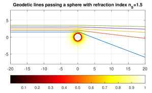
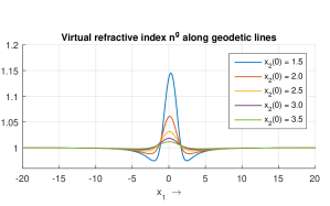
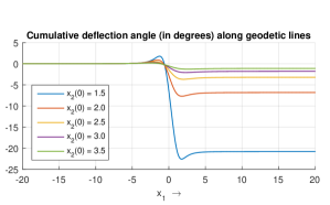
Figure 1: Top figure: Geodetic lines in presence of a homogeneous sphere of radius of 1, starting in the $(x_{1},x_{2})$-plane at $x_{1}(0)=-20$, for various values of $x_{2}(0)$. The refractive index $n_{S}$ of the sphere is 1.5. All coordinates are normalized with respect to the radius $R_{\cal S}$. To indicate the region where the virtual refractive index is effective, we have included an image of the quantity $1-(R_{\cal S}/R)^{2}$. The colorbar indicates these values. Middle figure: The virtual refractive index ${n^{\rm g}}$ as function of $x_{1}$ along the geodetic lines plotted in the top figure. Bottom Figure: The cumulative deflection angles in degrees as function of $x_{1}$ along the geodetic lines plotted in the top figure.

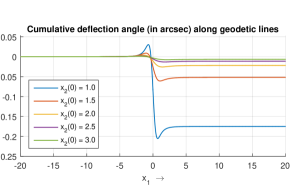
Figure 2: Same as Fig. 1, but now for a refractive index $n_{S}-1=0.53\times 10^{-6}$ and a different set of $x_{2}(0)$. In the middle figure, the vertical axis represents the values of the virtual refraction index ${n^{\rm g}}-1$. In the bottom figure, the angles are given in arcseconds.

In FIG. 1, we show some numerical results of geodetic lines constructed for $n_{\cal S}=1.5$. In its top figure, the phenomenon of bending of the geodetic lines located outside the sphere is clearly visible. We also applied the construction of these geodetic lines with a predictor-corrector method and we did not observe visible differences. To gain some insight on the influence of the virtual refractive index on the course of the geodetic path, we picture in the middle figure its value along the path. Approaching the sphere, the virtual velocity $v=c_{0}/{n^{\rm g}}$ increases and the geodetic line bends away from the sphere. Subsequently, the virtual velocity decreases in the radial direction and the geodetic line bends towards the sphere. The curvature of the wave fronts in the bottom figure of Fig. 1 agrees with this phenomenon. We observe that the presence of the sphere is noticeable in the horizontal range of $(-5R_{\cal S},5R_{\cal S})$. Outside this range the virtual refractive index tends to 1 and the geodetic lines become straight. In the bottom figure, we present the cumulative deflection angles for the different geodetic paths.

In FIG. 2, we mimic the bending of light by the Sun. The mean refractive index of the Sun is close to one. For grazing incidence, its value is chosen such that a total deflection angle of 1.75 arcsec is obtained. This is equivalent by taking $n_{\cal S}=1+0.53\times 10^{-6}$. A comparison with FIG. 1 shows that in the top figure of FIG. 2 the deflection of the geodetic lines is hardly visible. The same applies for the shift of the maximum values of the virtual refractive index in the middle figure. The curves are now almost symmetric with respect to $x_{1}$. In the bottom figure of FIG. 2, we present the cumulative deflection angle in arcsec. Comparing this picture with the bottom picture of FIG. 1, apart of their amplitudes, the global spatial behavior is similar.

Asymptotic analysis for small tension

We take advantage of the very small deflection angles of the geodetic lines outside the sphere. We integrate the differential equation for the geodetic line analytically, after making some appropriate approximations for refractive indices close to one and small deflection angles. We start with the expression for $A$ of Eq. (37). For small values of $n_{\cal S}\!-\!1$, we only retain the terms linear in $f_{R}$, i.e.,

$$A=(n_{\cal S}\!-\!1)\left[-3+9\cos^{2}(\theta\!-\!\alpha)\right]\frac{R_{\cal S}^{3}}{R^{4}}\,.$$ (39)

Further, in the region around the sphere, where $\theta$ has values around $\theta=\frac{1}{2}\pi$, we neglect the influence of $\alpha$. Outside this region, the values of $A$ become negligible. Next we consider the relation for $\alpha$ of Eq. (38). Within our approximations already made, we take $\sin\alpha\approx\alpha$, $\cos(\theta\!-\!\alpha)\approx\cos\theta$ and ${n^{\rm g}}\approx 1$. Subsequently, we expand the quotient of step (2a) of Eq. (38) in terms of small $\Delta s$ to obtain the cumulative deflection angle,

$$\alpha:=\alpha+(\partial_{2}{n^{\rm g}}-\partial_{1}{n^{\rm g}})\,\Delta s\approx\alpha+\left[A\sin\theta-A\cos\theta\right]\Delta s\,,$$ (40)

where we have used Eq. (36). With $\Delta s\approx\Delta x_{1}$ and similar type of approximations made before, the updates for the spatial coordinates become

$$x_{2}\approx x_{2}(0)\;\;{\rm and}\;\;x_{1}:=x_{1}+\Delta x_{1}\,.$$ (41)

Since $x_{2}$ is considered to be constant, we write the radial coordinate as $R=x_{2}(0)/\sin\theta$. The asymptotic expression for $A$ becomes

$$A\approx(n_{\cal S}\!-\!1)\left[-3+9\cos^{2}\theta\right]\frac{R_{\cal S}^{3}}{x_{2}^{4}(0)}\sin^{4}\theta\,.$$ (42)

Combining all these approximations, we observe that Eqs. (40) and (41) represent the numerical counterpart to calculate the following integral for the total deflection in the negative $x_{2}$-direction as:

$$d^{\rm EM}=-\!\int_{-\infty}^{\infty}\left[A\sin\theta-A\cos\theta\right]{\rm d}x_{1}=-2\!\int_{0}^{\infty}\!\!A\sin\theta\,{\rm d}x_{1},$$ (43)

because the first term of the integrand is a symmetric function of $x_{1}$, while the second one is asymmetric. Further, from $x_{1}=x_{2}(0)/\tan\theta$ follows that $\sin^{2}\theta\,{\rm d}x_{1}=-x_{2}(0)\,{\rm d}\theta$, and the integral is rewritten as

$$d^{\rm EM}=2(n_{\cal S}\!-\!1)\left[\frac{R_{\cal S}}{x_{2}(0)}\right]^{3}\int_{0}^{\frac{1}{2}\pi}\left[3-9\cos^{2}\theta\right]\sin^{3}\theta\,{\rm d}\theta\,.$$ (44)

The integral can be calculated analytically and is equal to 4/5. The asymptotic formula for the total deflection is finally obtained as

$$d^{\rm EM}=\frac{8}{5}(n_{\cal S}\!-\!1)\frac{1}{(R_{0}/R_{\cal S})^{3}}\,,\quad\;{\rm for\ small}\;\ n_{\cal S}\!-\!1\,,$$ (45)

where $R_{0}\approx x_{2}(0)$ is the smallest value of $R$ on the geodetic line. The value of $R_{0}/R_{\cal S}$ is often denoted as the impact parameter.

Table 1: Ratio $d^{\rm EM}_{\rm num}/d^{\rm EM}_{\rm asymp}$ of numerical values for total deflection angles and their small-tension approximations

		$\displaystyle n_{\cal S}\!-\!1\!=\!10^{-2}$		$\displaystyle n_{\cal S}\!-\!1\!=\!10^{-3}$		$\displaystyle n_{\cal S}\!-\!1\!=\!10^{-4}$
$R_{0}/R_{\cal S}$		1.02799		1.00278		1.00028
$R_{0}/R_{\cal S}$		1.00831		1.00086		1.00012
$R_{0}/R_{\cal S}$		1.00360		1.00046		1.00014
$R_{0}/R_{\cal S}$		1.00206		1.00044		1.00028
$R_{0}/R_{\cal S}$		1.00158		1.00064		1.00055

Figure 3: Left figure: The GR deflection (black line) and the linear superposition of GR and EM deflection by the tension of Sun’s interior refractive index (red line). The red squares denote the data given by Merat et al Merat et al. (1974). Middle figure: The linear superposition of GR deflection and deflection caused by the Corona (blue dashed line). Right figure: The linear superposition of the GR deflection, the EM deflection caused by the tension of the Sun and the one caused by the Corona (green line).

In TABLE 1, we present the values for the ratio of the deflection angle obtained numerically ($d^{\rm EM}_{\rm num}$) and the one obtained analytically ($d^{\rm EM}_{\rm asymp}$) using the asymptotic approximations. We note that the closer this ratio is to one, the better the asymptotic approach. We observe that the discrepancies in the approximations are of the order of $n_{\cal S}\!-\!1$. For increasing values of $R$ the approximations improve as well; the worst case appears for grazing incidence ($R_{0}/R_{\cal S}=1$); but we may conclude that, for values of $n_{\cal S}\!-\!1<10^{-3}$, the approximation is fully justified. Note that for the Sun case, deflection angles of the order of 1.75 arcsec are arrived at, which correspond to $n_{\cal S}\!-\!1\approx 10^{-6}$. Hence, there is no doubt about the validity of our asymptotic analysis.

From Eq. (45) we conclude that deflection angle is proportional to $(R_{0}/R_{\cal S})^{-3}$, while general relativity predicts a dependency of $(R_{0}/R_{\cal S})^{-1}$, see Fig. 1 of Biswas et al Biswas and Mani (2004). For convenience, we denote the electromagnetic contribution, the near-field term of the bending, while the gravitational contribution dominates the far-field term.

VI Validation on historical data

At this point, we return to the work of Merat et al Merat et al. (1974). They conclude on basis of radio deflection observations Muhleman et al. (1970), that for $R_{0}<5\,R_{\cal S}$ deviations from the Einstein prediction become statistically significant. They have collected the whole set of star deflection data into 4 samples. The weighted mean of the distance $R_{0}/R_{\cal S}$ of each sample has been given, together with the mean deviation of light deflections from the GR prediction. In FIG. 3, the red squares denote the total deflection data values, including the GR predictions. In the left picture of FIG. 3, the GR curve itself is shown as the black curve. The differences of the data with the GR curve are the four data points given in Table 3 of Merat et al Merat et al. (1974). For decreasing $R_{0}/R_{\cal S}$, the discrepancies with the GR prediction increase. The discrepancies between the four data points and this black curve amounts to 0.139, 0.081, 0.023 and 0.013, respectively. The mean square of these residuals with respect to the total deflection error amounts to 31 %.

VI.1 Influence of the EM tension

To improve the GR reflection model, we assume that the total deviation data is a linear superposition of the GR curve $(R_{0}/R_{\cal S})^{-1}$ and our EM curve $(R_{0}/R_{\cal S})^{-3}$. We define

$$d^{\rm EM}=d^{tot}-\frac{1.75\,{\rm arcsec}}{(R_{0}/R_{\cal S})}=\frac{B}{(R_{0}/R_{\cal S})^{3}}\,.$$ (46)

To find the unknown factor $B$, we carry out a least-square fit, which minimizes the deviations and the four data points of Merat et al. (1974). Substituting the resulting value of $B$ in Eq. (46), the total deflection function $d^{\rm GR}+d^{\rm EM}$ is presented as the red line in the left picture of FIG. 3. The discrepancies between the four data points and this red curve amounts to -0.0107, 0.0549, 0.0137 and 0.0091, respectively. The mean square of these residuals with respect to the total deflection error amounts to 14 %. These discrepancies with respect to the four data points may be explained as a Corona effect outside the domain ${\cal S}$ of the Sun.

VI.2 Influence of the Corona

In the Corona, we only take into account the local effect of the refractive index of the Corona. In order to include the plasma effects of the Corona, we start with the refractive index described as a superposition of powers of $R_{\cal S}/R$, with constant factors $\eta_{p}$, viz.

$$n_{\cal C}(R)-1=\sum_{p}\eta_{p}\Bigl{(}\frac{R_{\cal S}}{R}\Bigr{)}^{p}\,,\quad p>1,\quad R>R_{\cal S}\,.$$ (47)

The data under consideration are obtained for $R>3R_{S}$ and we employ the refractive index described in Muhleman et al. (1970), viz.,

$$n_{C}(R)-1=\eta_{p_{1}}\Bigl{(}\frac{R_{\cal S}}{R}\Bigr{)}^{p_{1}}+\eta_{p_{2}}\Bigl{(}\frac{R_{\cal S}}{R}\Bigr{)}^{p_{2}}\,,\quad\frac{R_{\cal S}}{R}>3\,,$$ (48)

where $p_{1}=6$ and $p_{2}=2.33$. Using the results of Appendix B, the electromagnetic deflection is obtained as

$$d^{EM}=\frac{C_{p_{1}}}{(R_{0}/R_{\cal S})^{p_{1}}}+\frac{C_{p_{2}}}{(R_{0}/R_{\cal S})^{p_{2}}}\,.$$ (49)

For the range of $R_{0}>3R_{\cal S}$ we determine the coefficients $C_{p_{1}}$ and $C_{p_{2}}$ by a least-square fitting of Eq. (49) to the four data points given by Merat et al Merat et al. (1974).

In the middle picture of FIG. 3, the deflection by the local coronal medium is presented as the blue dashed line. The discrepancies between the four data points and this blue dashed curve are -0.0002, 0.0071, -0.0119 and -0.0048, respectively. The mean square of these residuals with respect to the total deflection error amounts to 5 %.

VI.3 Influence of the EM tension and the Corona

In the integral expression of $f_{R}$, see Eq. (24), for $R>R_{\cal S}$, we subtract in the integrand $n(r)\!-\!1$ the coronal contribution, $n_{\cal C}(r)\!-\!1$, so that the integral is restricted to the range of $0<r<R^{S}$. Then, the EM deflection is given by Eq. (46). Following the pure gravity light bending theory of Maccone Maccone (2009), we also denote this as the naked-Sun situation. For small deflections, we take a linear superposition of the naked-Sun part and the mantle part (the Corona). We conclude that the total electromagnetic deflection may be written as

$$d^{EM}=\frac{B}{(R_{0}/R_{\cal S})^{3}}+\frac{C_{p_{1}}}{(R_{0}/R_{\cal S})^{p_{1}}}+\frac{C_{p_{2}}}{(R_{0}/R_{\cal S})^{p_{2}}}\,.$$ (50)

In a least-square fitting procedure to the data, we observed that the system matrix is heavily ill-posed and impossible to invert numerically. A stable result is obtained by preconditioning. We rewrite Eq. (50) as

$$d^{EM}=\frac{B}{(R_{0}/R_{\cal S})^{3}}\left[1+\frac{C_{1}}{(R_{0}/R_{\cal S})^{p_{1}-3}}+\frac{C_{2}}{(R_{0}/R_{\cal S})^{p_{2}-3}}\right],$$ (51)

where $C_{1}=C_{p_{1}}/B$ and $C_{2}=C_{p_{2}}/B$. This nonlinear equation is solved with an iterative Gauss-Newton method. As starting values we take zero values for $C_{1}$ and $C_{2}$ and determine $B$ by a direct least-square minimization. After carrying out a few Gauss-Newton iterations a stable result is obtained. The resulting deflection is plotted as the green line in the right picture of Fig. 3. The discrepancies between the four data points and this red curve amounts to -0.0000, 0.0008. -0.0036 and 0.0040, respectively. The mean square of these residuals with respect to the total deflection error amounts to 2 %. In comparison with the deviation as sum of the GR and Corona constituents, the present global error has been halved by more than a factor of two.

Table 2: Parameters $B$, $C_{p_{1}}$ and $C_{p_{2}}$ (in arcsec) substituted into Eq. (51) to plot the three curves of Fig. 4. For convenience we also present the ratio of $C_{p_{1}}/C_{p_{2}}$.

		naked Sun		mantle		naked Sun $\!+\!$ mantle
		(red curve)		(blue dashed)		(green curve)
$B$		6.04		0		36.8
$C_{p_{1}}$		0		-274		$-3.17\times 10^{4}$
$C_{p_{2}}$		0		5		$-1.59\times 10^{2}$
$C_{p_{1}}/C_{p_{2}}$		-		-50		199

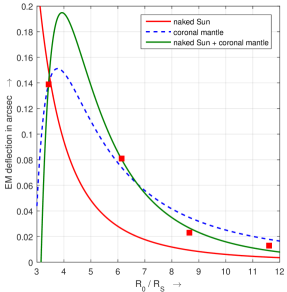
Figure 4: Details of the additional EM deflection in a vacuum medium as function of $R_{0}/R_{\cal S}$. The red line is the deflection result due to the tension of Sun’s interior, without the Corona (naked Sun). The blue dashed line is the deflection result due to propagation of the wave through the Corona only (coronal mantle). The green line denotes the deflection result due to the tension of Sun’s interior and the bending of light through a coronal medium (naked Sun + coronal mantle). The red squares denote the data given by Merat et al Merat et al. (1974).

To judge the value of the different results, in Table 2 we present the values of the three parameters $B$, $C_{p_{1}}$ and $C_{p_{2}}$ obtained from our three fitting procedures. Also the differences between the results of Fig. 3 becomes more visible when we only present the electromagnetic parts of the deflection $d^{\rm EM}$, see Fig. 4. Although the blue dashed and green curve have a similar shape, their parameters $C_{p_{1}}$ and $C_{p_{2}}$ are completely different. Note that the ratio $C_{p_{1}}/C_{p_{2}}=199$, obtained in the fourth column, is close to a similar ratio of 228/1.1 = 207, determined empirically by Turyshev and Andersson Turyshev and Andersson (2003). When we neglect the refractional tension ($B=0$), we observe in the third column a negative ratio $C_{p_{1}}/C_{p_{2}}$, which seems in contradiction to other historical data, e.g. Muhleman et al. (1970). Under condition that we keep the GR prediction unchanged, we claim that the near-field correction due to the tension of the Sun’s interior refractive index is a prerequisite to obtain an accurate model in solar gravitational lensing Eshleman (1979); Maccone (2009).

VI.4 Frequency dependent bending

Consistent with the frequency dependent refractive index $n_{\cal C}=n_{\cal C}(\omega)$ of the coronal medium also the interior refraction index $n_{\cal S}=n_{\cal S}(\omega)$ of the Sun is frequency dependent. The additional EM deflection $d^{\rm EM}$ is linearly related to these frequency-dependent refractive indices. As far as the frequency-dependent refractive index of Sun’s interior is concerned, the outer layer can be represented by a refractive index that differs from the other inner layers. This will change its mean value $n_{\cal S}$.

VII Conclusions

In this paper we demonstrated that apart from a gravitational type and a coronal type of bending along the Sun, Maxwell’s equations predict an additional type of bending by the existence of a refractional tension. The latter is caused by the presence of a non-zero refractive index of the Sun’s interior medium. This electromagnetic addition to the GR tension has been verified on data from historical astrophysical measurements without changing the GR tension. It has been shown that the additional EM tension is an essential ingredient of the prediction of the interstellar wave propagation paths. The influence of the refractional tension becomes more significant for observations closer to the Sun.

The electromagnetic deflection (including the coronal one) is frequency-dependent and dominant in the near- and mid-field, while the GR contribution is frequency independent and it dominates the far-field. Future research is extremely important for gravity lensing and interstellar communication experiments, where accurate electromagnetic predictions of possible interstellar pathways are sought.

We conclude our paper by mentioning that a scaled experiment is possible by using a voluminous object with a noticeable refractive index. This will potentially verify the electromagnetic deflection outside the object, since the gravitational and coronal components can be neglected in this case.

Appendix A The refractional potential and the tension for a radially inhomogeneous sphere and its derivatives

For a radially inhomogeneous sphere, the refractional potential of Eq. (17) can be calculated analytically. We introduce spherical coordinates for the observation points $x$ as

$$x_{1}=R\sin\theta\cos\phi\,,\>x_{2}=R\sin\theta\sin\phi\,,\>x_{3}=R\cos\theta\,,\>$$ (52)

and spherical coordinates for the integration points $\mbox{{\boldmath$x$}}^{\prime}$ as

$$x_{1}^{\prime}=r\sin\theta^{\prime}\cos\phi^{\prime}\,,\>x_{2}=r\sin\theta^{\prime}\sin\phi^{\prime}\,,\>x_{3}=r\cos\theta^{\prime}\,.$$ (53)

For convenience we take the polar axis in the direction of $x$. Then, the Cartesian distance and the volume element become

$$\begin{array}[]{rcl}|\mbox{{\boldmath$x$}}-\mbox{{\boldmath$x$}}^{\prime}|&=&[R^{2}+r^{2}-2\,R\,r\cos\theta^{\prime}]^{\frac{1}{2}}\,,\\[5.69054pt] {\rm dV}&=&r^{2}\sin\theta^{\prime}\,{\rm d}r\,{\rm d}\theta^{\prime}\,{\rm d}\phi^{\prime}\,.\end{array}$$ (54)

In the resulting integral we first carry out the integration with respect to $\phi^{\prime}$; this merely amounts to a multiplication by a factor of $2\pi$, so that Eq. (17) transfers into

$$\Phi(R,\theta,\phi) = \frac{3}{2}\int_{0}^{\infty}\![n(r)-1]\,{\rm}r^{2}\,{\rm d}r$$

$$\hskip 14.22636pt\int_{0}^{\pi}\!\!\frac{\sin\theta^{\prime}}{[R^{2}\!+\!r^{2}\!-\!2Rr\cos\theta^{\prime}]^{\frac{1}{2}}}{\rm d}\theta^{\prime}\,.$$

Next we carry out the integration with respect to $\theta^{\prime}$, which is elementary. After this, we have

$$\Phi(R,\theta,\phi)=\frac{3}{2}\int_{0}^{\infty}[n(r)-1]\,r^{2}\left[\frac{R+r}{Rr}-\frac{|R-r|}{Rr}\right]\,{\rm d}r\,,$$ (55)

which shows that $\Phi$ is independent of $\theta$ and $\phi$. Taking into account the meaning of $|R-r|$, we obtain

$$\Phi(R)=\frac{3}{R}\int_{0}^{R}{\rm}[n(r)-1]\,r^{2}\,{\rm d}r+3\int_{R}^{\infty}[n(r)-1]\,r\,{\rm d}r\,.$$ (56)

Note that this expression holds for all $R$, if $n(r)=O(r^{-2})$ when $r$ tends to infinity.

The gradient of the potential is directed in the radial direction. Hence $\nabla\Phi=(d\Phi/dR)\,{\bf i}_{R}$. Applying Leibniz’ rule for differentiation of an integral to Eq. (56) yields

$$\frac{d\Phi}{dR} = -\frac{3}{R^{2}}\int_{0}^{R}[n(r)-1]\,r^{2}\,{\rm d}r$$ (57)

$$\hskip 28.45274pt+\frac{3}{R}[n(R)-1]\,R^{2}-3[n(R)-1]\,R\,,$$

which simplifies to

$$\frac{d\Phi}{dR}=-\frac{3}{R^{2}}\int_{0}^{R}[n(r)-1]\,r^{2}\,{\rm d}r\,.$$ (58)

With this result, the tension $\mbox{{\boldmath$f$}}=f_{R}{\bf i}_{R}=-({d\Phi}/{dR})\,{\bf i}_{R}$ is obtained as

$$f_{R}(R)=\frac{3}{R^{2}}\int_{0}^{R}[n(r)-1]\,r^{2}\,{\rm d}r\,.$$ (59)

Appendix B Deflection due to presence of the Corona

Let us consider the coronal refractive index for a particular term in which the radial dependence is given a certain inverse power of $p$, viz.,

$$n_{C}(R)=1+\eta_{p}\Bigl{(}\frac{R_{\cal S}}{R}\Bigr{)}^{p}\,,$$ (60)

Then, the partial derivatives with respect to $x_{1}$ and $x_{2}$ are obtained as

$$\partial_{1}n_{C}=\frac{x_{1}}{R}\partial_{R}n_{C}\,,\quad\partial_{2}n_{C}=\frac{x_{2}}{R}\partial_{R}n_{C}\,,$$ (61)

where

$$\partial_{R}n_{C}(R)=-\eta_{p}\,p\,\frac{R_{\cal S}^{p}}{R^{p+1}}\,.$$ (62)

Similar as before, for small values of $\eta$, the cumulative deflection angle is given by

$$\alpha : =\alpha+(\partial_{2}n_{C}-\partial_{1}n_{C})\,\Delta s$$ (63)

$$=\alpha-\eta_{p}\,p\,\frac{R_{\cal S}^{p}}{R^{p+1}}(\sin\theta-\cos\theta)\Delta s\,,$$

and the total deflection caused by the presence of the Corona becomes

$$d^{\rm EM}=-\eta_{p}\,p\left[\frac{R_{\cal S}}{x_{2}(0)}\right]^{p}F(p)\,,$$ (64)

in which

$$F(p) = \int_{0}^{\pi}\!\!\!\left[\sin^{p}\!\theta\!-\!\sin^{p}\,\!\!\theta\,\cos\theta\right]\!{\rm d}\theta=2\!\int_{0}^{\frac{\pi}{2}}\!\!\sin^{p}\!\theta\,{\rm d}\theta$$ (65)

$$= \frac{\sqrt{\pi}\,\Gamma(\frac{1}{2}+\frac{1}{2}p)}{\Gamma(1+\frac{1}{2}p)}\,.$$