Quantum error correction and entanglement spectrum in tensor networks

Abstract

A sort of planar tensor networks with tensor constraints is investigated as a model for holography. We study the greedy algorithm generated by tensor constraints and propose the notion of critical protection (CP) against the action of greedy algorithm. For given tensor constraints, a CP tensor chain can be defined. We further find that the ability of quantum error correction (QEC), the non-flatness of entanglement spectrum (ES) and the correlation function can be quantitatively evaluated by the geometric structure of CP tensor chain. Four classes of tensor networks with different properties of entanglement is discussed. Thanks to tensor constraints and CP, the correlation function is reduced into a bracket of Matrix Production State and the result agrees with the one in conformal field theory.

I Introduction

Quantum entanglement plays a key role in understanding the structure of spacetime from the emergent point of view Maldacena:2001kr ; VanRaamsdonk:2010pw . The Ryu-Takayanagi (RT) formula links the entanglement entropy of a subsystem on the boundary to the area of the minimal homological surface in the bulk Ryu:2006bv . Such an approach has been recently generalized to construct the gravitational dual of Renyi entropy Dong:2016fnf , which provides a correspondence of entanglement spectrum (ES) between the bulk and the boundary. In particular, for the vacuum in $AdS_{3}/CFT_{2}$ correspondence, Renyi entropy satisfies Cardy-Calabrese formula and a non-flat ES is inherent Calabrese:2004eu ; Calabrese:2009qy . Another remarkable feature of AdS space is the subsystem duality, which states that a local operator in the bulk can be reconstructed in a subsystem $A$ on the boundary if it is located within the entanglement wedge of $A$ Hamilton:2006az ; Dong:2016eik ; Cotler:2017erl ; Freivogel:2016zsb ; Mintun:2015qda ; Almheiri:2014lwa ; Harlow:2018fse . It can be be viewed as the accomplishment of Quantum Error Correction (QEC) in quantum information Schumacher:1996dy ; Almheiri:2014lwa ; Pastawski:2015qua ; Harlow:2018fse . Moreover, it is found that RT formula can be derived from QEC Harlow:2016vwg .

It has been revealed that tensor networks provide a geometric picture for entanglement renormalization such that holographic spaces may emerge from the entanglement of a many-body systemVidal:2007hda ; Swingle:2009bg ; Swingle:2012wq , gearing up the exploration on the deep relation between tensor networks and the structure of spacetime Nozaki:2012zj ; Qi:2013caa . One typical kind of tensor networks is the multiscale entanglement renormalization ansatz (MERA), which respects RT formula, exhibiting logarithmic law of entanglement entropy and non-flat entanglement spectrum as the AdS vacuum Vidal:2007hda ; Swingle:2009bg ; Swingle:2012wq ; Kim:2016wby ; Bao:2015uaa . However, MERA breaks the isometry group $SL(2,R)$ and has a preferred direction, implying that QEC can not be realized along all directions. On the other hand, perfect tensors, which are also called as holographic codes, take the advantages of implementing QEC over a $H^{2}$ space Pastawski:2015qua ; Yang:2015uoa ; Donnelly:2016qqt . Unfortunately, it is found that such kind of tensor networks has a flat ES and trivial connected correlation functions, which evidently is not a reflection of the holographic property of AdS spacetime Bhattacharyya:2016hbx ; Evenbly:2017htn . In random tensor networks and spin networks, all the orders of Renyi entropy for the ground state share the same RT formula, leading to a flat ES as well Hayden:2016cfa ; Qi:2018shh ; Chirco:2017wgl ; Han:2016xmb . The attempt to recover the result of Cardy-Calabrese formula of Renyi entropy, $S_{n}=(1+1/n)(c/6)\log(l/\epsilon)$, can be found in Han:2017uco where the bulk dynamics is taken into account.

Recently a new class of tensor networks which is named hyperinvariant tensor networks has been constructed in Evenbly:2017htn , which retains the advantages of both MERA and perfect tensor networks. The key ingredient of hyperinvariant tensor networks is to impose multi-tensor constraints, which demand certain product of multiple tensors to form an isometric mapping. Remarkably, this sort of tensor networks can not only accomplish QEC as perfect tensors, but also generate non-flat ES as MERA, thus qualitatively capturing both holographic features of AdS spacetime.

Nevertheless, some key issues remain unanswered in this approach. First of all, the holographic property of tensor networks depends on the specific structure of tensor constraints. What kind of multi-tensor constraints could endow desirable features of AdS spacetime to a given tensor network? More importantly, to accomplish the holographic features of tensor networks one always faces a dilemma: once the ability of QEC of a tensor network becomes stronger, then more easily its ES becomes flat, and vice versa. Is there any criteria to characterize the ability of QEC and the non-flatness of ES for a tensor network with given constraints? At the same time, can any feature of CFT be reflected by the specific structure of tensor networks? We wish to answer above issues based on some examples of tensor network.

We will construct tensor networks by tiling $H^{2}$ space with identical polygons, and then impose tensor constraints with the notion of tensor chain, which leads to a generalized description of greedy algorithm. We will investigate QEC, ES and correlation function by manipulating tensor networks. For the ES and correlation function, we will also compare our holographic results with the results in conformal field theory. Moreover, we will propose the notion of critical protection (CP) to describe the behavior of tensor networks under the greedy algorithm. A geometric quantity $\kappa_{c}$, named as the average reduced interior angle of a tensor chain, will be proposed to measure the ability of QEC and justify the flatness of ES.

II Constraints on tensor chains

II.1 Tensor Chains

We discretize $H^{2}$ space uniformly by gluing identical polygons composed of $b$ edges, with $a$ edges sharing the same node. We call such discretization as the $\{b,a\}$ tiling of $H^{2}$ space. Since the sum of interior angles of a triangle in a space with negative curvature must be less than $2\pi$, a $\{b,a\}$ tiling of $H^{2}$ space can be realized only if $\frac{1}{a}+\frac{1}{b}<\frac{1}{2}$.

A tensor network can be constructed based on each $\{b,a\}$ tiling, as illustrated in Fig. 2. Associated with each node, we define a tensor $T$ with $a$ indexes, each of which is specified to an edge jointed at the node respectively. Associated with each edge, we define a tensor $E$ with $2$ indexes. Because of the rotational invariance of $H^{2}$ space, we demand that the indexes of tensor $T$ and $E$ have cyclic symmetry

$$T^{i_{1}i_{2}\cdots i_{a}}=T^{i_{2}i_{3}\cdots i_{a}i_{1}},\quad E_{i_{1}i_{2}}=E_{i_{2}i_{1}}.$$ (1)

Consider a tensor network $\Psi$, and let all the indexes of tensors $T$ contract with those of tensors $E$ such that all uncontracted indexes belong to tensors $E$ only. Corresponding to such a network, we define a state $\left|\Psi\right\rangle$ in the Hilbert space on those uncontracted edges.

By dissecting a tensor network, as in Fig. 2, we define a key object called tensor chain $M$, whose general form is shown in Fig. 2. Vividly, the uncontracted edges in $M$ are split into the upper part $A$ and lower part $B$. So we denote its elements as $M^{A}_{B}$. The number of edges at each node satisfies $m_{i}+n_{i}=a-2+\delta_{i1}+\delta_{ik}$, where $i$ is the sequence number labelling the node of tensor chain. Specifically, for the tensor chain in Fig. 2, $k=4,\,\left(m_{1},m_{2},m_{3},m_{4}\right)=\left(2,0,1,1\right),\,\left(n_{1},n_{2},n_{3},n_{4}\right)=\left(1,2,1,2\right)$.

Vice versa, a tensor chain can be mapped into the tiling of $H^{2}$ space and its skeleton forms a directed polyline in the network, where along the direction of the polyline the sequence number $i$ increases and the upper (lower) edges are placed on the left (right) hand side of the polyline. To describe the curvature of its corresponding polyline, we define the average reduced interior angle of a tensor chain as

$$\kappa=\frac{1}{k}\left(\sum_{i=1}^{k}m_{i}+k-1\right),$$ (2)

where “reduced” means that we have taken ${2\pi\over a}$ as the unit of interior angles.

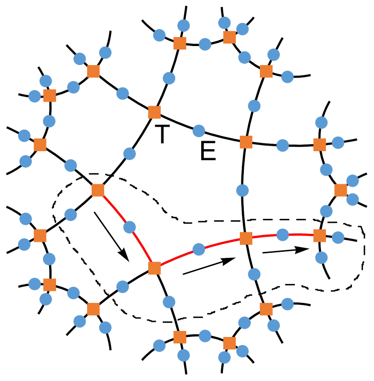
Figure 1: A tensor network with $\left\{5,4\right\}$ tiling. Enclosed by the dashed line is an example of tensor chain. Its skeleton forms a directed polyline which is marked in red.

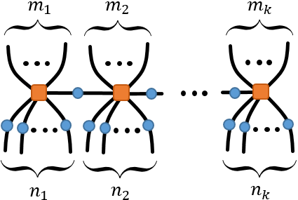
Figure 2: A general form of tensor chain.

We will focus on the tensor network with $\left\{5,4\right\}$ tiling as a typical example to disclose the structure of the tensor chain which is critically protected under the action of greedy algorithm. Our analysis and results can be generalized to the tensor networks with $\left\{a,b\right\}$ tiling.

II.2 Tensor Constraints

II.2.1 Tensor network with $\kappa_{c}=2$

We define tensor constraints as follows. Besides the cyclic symmetry, we further impose constraints on rank-$4$ tensor $T$ (orange square) and rank-$2$ tensor $E$ (blue circle), such that they satisfy the following equations

$$\includegraphics[height=30.35216pt]{541TC.png}\quad,\quad\includegraphics[height=30.35216pt]{542TC.png},$$ (3)

where the conjugation of tensors are marked in dark colors. In other words, the tensor chains

$$\includegraphics[height=25.29604pt]{542PITC.png}.$$ (4)

are proportional to isometries from the Hilbert space on upper edges to the Hilbert space on lower edges. For convenience, in the remainder of this paper we will adopt the expression like (4) to represent tensor constraints for short. The shape of the tensor chain in constraints (4) can be characterized by their average reduced interior angle, which is $\left\{1/1=1,~{}2/1=2\right\}$. We will call the maximal one as the CP reduced interior angle $\kappa_{c}=2$, as the reason will become clear later.

For the simple case as illustrated in (4), each of tensor chains only involves a single tensor $T$. One can derive other tensor chains proportional to isometries as well from the tensor constraints. For instance, from (4), the following tensor chains are proportional to isometries.

$$\includegraphics[height=25.29604pt]{54_11_21.png}.$$ (5)

The detailed analysis is given in Ling:2018ajv . Here we just argue that all of these tensor chains form a set $S_{D}$ with infinite number of elements, and satisfy $\kappa\leq\kappa_{c}$. The subscript $D$ refers to the fact that $S_{D}$ is derived from tensor constraints given. We stress that one should take all these tensor chains into account when justifying whether the contraction of tensor product could be simplified under the action of greedy algorithm.

We further require that any tensor chain which is proportional to isometry can be derived from tensor constraints, which restricts the structure of tensor $T$ and $E$. In other words, we require that those tensor chains which do not belong to the set $S_{D}$ should not be propositional to isometries, which prevents tensor $T$ and $E$ from trivial structure, for instance, the outer product of identity matrices. We point out that many tensor chains do not belong to $S_{D}$, such as the following tensor chains for constraints (4)

$$\includegraphics[height=25.29604pt]{54_3_22.png},$$ (6)

II.2.2 Tensor network with $\kappa_{c}=3/2$

Definitely, we may impose other tensor constraints, for instance, by requiring the following tensor chains to be proportional to isometries.

$$\includegraphics[height=25.29604pt]{5411PITC.png},$$ (7)

whose average reduced interior angles are $\left\{1,3/2\right\}$, then $\kappa_{c}=3/2$. Similarly, from (7), the following tensor chains are proportional to isometries

$$\includegraphics[height=25.29604pt]{54_10_101.png},$$ (8)

but the following tensor chains are not

$$\includegraphics[height=25.29604pt]{54_2_21_111.png}.$$ (9)

The specific construction of tensors $T$ and $E$ subject to above constraints is given in Appendix A.

III Greedy Algorithm and Protection

III.1 General Greedy Algorithm with Tensor Chain

We firstly review the greedy algorithm on a tensor network following the description in Pastawski:2015qua , which provides an intuitive way to figure out the region in which the corresponding sub tensor network must be an isometry. Beginning with an interval $A$ on the boundary of a tensor network $\Psi$, we consider a sequence of cuts $\left\{C_{n}\right\}$, each of which is bounded by $\partial A$ and obtained from the previous one by a local move on the lattice. The corresponding sub tensor networks also form a sequence of $\left\{\Phi_{n}\right\}$, where $\Phi_{n}$ consists of those tensors between $A$ and $C_{n}$. Let $C_{1}=A$ and $\Phi_{1}$ is an identity. For perfect tensors, at each step one figures out a tensor $M_{n}$ which has at least half of its legs contracted with $\Phi_{n}$ and construct $\Phi_{n+1}$ by adding $M_{n}$ to $\Phi_{n}$ such that $\Phi_{n+1}$ must be an isometry as well. The procedure stops when one fails to add such tensors to the sequence.

We can generalize the above description by replacing its single tensor $M_{n}$ by a tensor chain $M_{n}$ which is proportional to isometry, with lower edges contracted with $\Phi_{n}$. According to section II.2, those tensor chains which are proportional to isometries form a set $S_{D}$ derived from tensor constraints.

Furthermore, we can generalize the target of greedy algorithm to a tensor chain $M$ rather than a tensor network $\Psi$. Given a tensor chain $M$, we simplify the contraction $\sum_{B}M_{B}^{A}(M_{B}^{C})^{*}$ subject to tensor constraints. For example, according to (3), we can simplify the contraction

$$\includegraphics[height=40.47212pt]{542GA31.png}.$$ (10)

Similarly, according to (5), we can simplify the contraction

$$\includegraphics[height=40.47212pt]{5411GA1003.png}.$$ (11)

Actually, the above description of greedy algorithm is equivalent to the description in Pastawski:2015qua for a single-interval. At each step from $\Phi_{n}$ to $\Phi_{n+1}$, a $M_{n}\in S_{D}$ is used to simplify a tensor chain $M$. For example, the procedure of simplifying (10) corresponds to the step of extending the shaded region as illustrated in Fig. 4, where the corresponding tensors are enclosed by dashed line in red. Similarly, the process of simplifying (11) corresponds to those steps in Fig. 4.

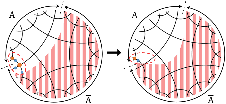
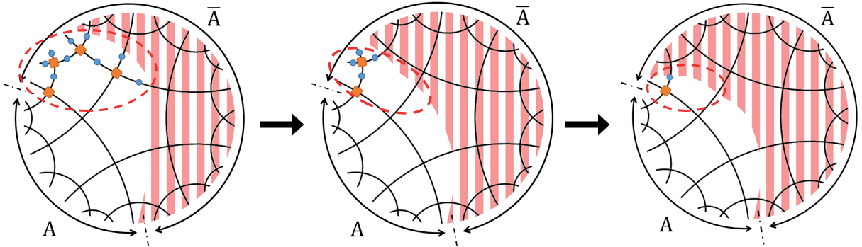
Figure 3: One step in the greedy algorithm generated from (3) beginning at $\bar{A}$.

Figure 4: Two steps in the greedy algorithm generated from (5) beginning at $\bar{A}$.

We define that a tensor chain $M$ is unprotected if it can be simplified under the action of greedy algorithm. Otherwise, say it is protected.

III.2 Critical Protection (CP)

Generally speaking, when the tiling and tensor constraints are given, the larger $\kappa$ is, the easier a tensor chain becomes unprotected. The protected and endless $M$ with largest $\kappa$ is called critically protected (CP) tensor chain $M_{c}$. Equivalently, one can check that $M_{c}$ would become unprotected once the list of its $n_{i}$ are rearranged or increased. Its $\kappa$ is called CP reduced interior angle $\kappa_{c}$.

Under the greedy algorithm generated by (4), if $\exists i$ s.t. $n_{i}>1$, then $M$ is unprotected. So CP tensor chain has the form as plotted on the right hand side of (12)

$$\includegraphics[height=25.29604pt]{542tran.png}\includegraphics[height=25.29604pt]{542CP.png}.$$ (12)

Here we have also presented a scheme to figure out CP tensor chain by a manipulation on the second constraint in (4). The skeleton of such a CP tensor chain forms a polyline in the tensor network, as shown in Fig. 6. For (12), $\kappa_{c}=2/1=2$, which is just equal to the maximal one of the average reduced interior angles of the tensor chains in constraints (4).

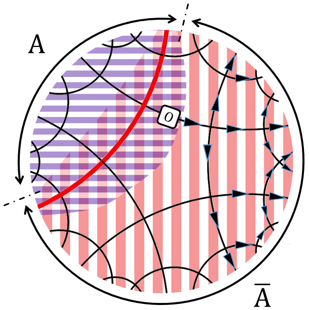
Figure 5: The tensor network with $\{5,4\}$ tiling and tensor constraints (4). Those tensors within the shaded region with purple (red) stripes is absorbed by the greedy algorithm starting from $A$ ($\bar{A}$). The CP tensor chain is marked by a solid line in red. An operator $O$ in the bulk is pushed to a sub-interval of $\bar{A}$.

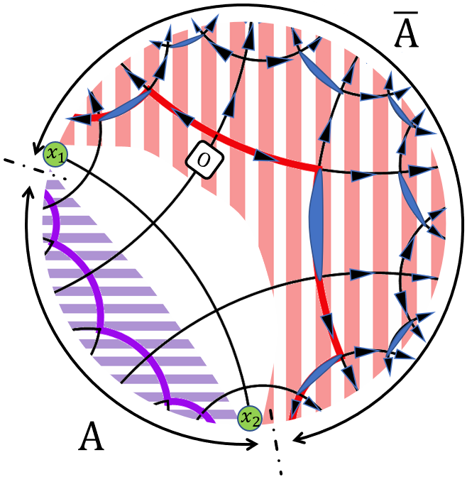
Figure 6: The tensor network with $\{5,4\}$ tiling and tensor constraints (7). The tensors in the blank region are not absorbed by the greedy algorithm. Two CP tensor chains correspond to thick polylines in purple and red, respectively. An operator $O$ enclosed by the CP tensor chain is pushed to a region within $\bar{A}$ on the boundary, where blue edges in the shape of rod indicate the employment of the second constraint in (7).

We deduce the CP tensor chain $M_{c}$ from constraints (7) as follows. From the first constraint, we know the number of lower edges at any node in CP tensor chain should be smaller than three; while from the second constraint, we know any two nodes with two lower edges can not be neighbored (otherwise they would be swallowed by the constraint). Therefore, $M_{c}$ has the form as plotted on the right hand side of (13)

$$\includegraphics[height=25.29604pt]{5411tran.png}\includegraphics[height=25.29604pt]{5411CP.png}.$$ (13)

Similarly, one can construct $M_{c}$ based on the second constraint in (7), as demonstrated in (13). The corresponding polyline in the network is marked in Fig. 6. The CP reduced interior angle is $\kappa_{c}=(1+2)/2=3/2$.

IV QEC and ES

Throughout this paper we will only consider the QEC by inserting an operator into the inter bonds, for instance,

$$\includegraphics[height=25.29604pt]{542in.png}.$$ (14)

By virtue of tensor constraints, one can push an operator $O$ ‘through’ tensor chains in (4) and turn into an operator $O^{\prime}$, namely

$$\includegraphics[height=25.29604pt]{542push13.png}\quad,\quad\includegraphics[height=25.29604pt]{542O13.png},$$ (15)

$$\includegraphics[height=25.29604pt]{542push22.png}\quad,\quad\includegraphics[height=25.29604pt]{542O22.png},$$ (16)

where the conjugation of tensors are marked in dark colors. Then one can realize the algorithm of QEC, as shown in Fig. 6. Actually, pushing an operator to an interval $\bar{A}$ on the boundary is the inverse of the greedy algorithm beginning at $\bar{A}$. So any operator inserted outside the CP tensor chain can be pushed to the boundary.

Next we consider the ES of the reduced density matrix

$$\rho_{A}=\frac{1}{Z}\mathrm{Tr}_{\bar{A}}{\left|\Psi\right\rangle\left\langle\Psi\right|}=\frac{1}{Z}\Psi\Psi^{\dagger},\quad Z=\left\langle\Psi|\Psi\right\rangle,$$ (17)

where $\bar{A}$ is contracted in the matrix production of tensor networks $\Psi$ and $\Psi^{\dagger}$, and the normalized factor $Z$ is obtained by contracting all the indexes between them. $\rho_{A}$ has a flat ES if all the non-zero eigenvalues are identical. From the diagonalization of $\rho_{A}$, we know that the flatness of ES is equivalent to

$$\rho^{2}_{A}\propto\Psi\Psi^{\dagger}\Psi\Psi^{\dagger}\propto\Psi\Psi^{\dagger}\propto\rho_{A},$$ (18)

which is also equivalent to state that all the orders of Renyi entropy are equal. If all the tensors are absorbed by the greedy algorithm starting from $A$ and from $\bar{A}$ respectively, then the relation in (18) holds and leads to a flat ES. Otherwise the ES is generally non-flat. When there exist tensors which are not absorbed by the greedy algorithm, although we can not exclude the tiny possibility that (18) happens to be valid for some construction of tensor $T$ and $E$ under fine-tuning, we still call that the ES is non-flat for a general construction of tensor $T$ and $E$.

We show the result of the greedy algorithm acting on the tensor network with constraints (4) in Fig. 6. It indicates that the ES is flat, which coincides with the results in Bhattacharyya:2016hbx . While for the tensor network with constraints (7), the ES is non-flat as shown in Fig. 6. At the same time, we point out that the ability of QEC in this network is weakened in comparison with that in the network with (4), because the operator inserted into the region enclosed by CP tensor chains will approach the endpoints of $A$ during the pushing process. Such phenomenon may be related to the approximate QEC Schumacher:2002aqe ; Almheiri:2014lwa .

The boundary effect in above analysis should be stressed. One may notice that CP tensor chain $M_{c}$ itself falls into the shaded region, implying that it is absorbed by the greedy algorithm. This phenomenon results from the boundary effect in a network with finite layers, where besides the lower edges of $M_{c}$, the edges at the end of $M_{c}$ need to be contracted as well. The boundary effect of greedy algorithm is investigated with details in Ling:2018ajv . Here we just remark that this effect is very limited, only swallowing finite layers (usually only one layer) of tensors enclosed by $M_{c}$.

Next we investigate the Renyi entropy $S_{n}$ for the tensor network composed of the tensors subjected to constraint Fig. 7. The specific construction of tensors $T$ and $E$ is given in Fig. 19, where elementary tensors $Q$ and $U$ satisfy the relation in (28). We numerically calculate $S_{n}$ for region $A$ in the tensor network in Fig. 6. The result is shown in Fig. 7, reflecting a non-flat ES. For a fixed region $A$, $S_{n}$ has a form of $\left(1+1/n\right)a+b$, which appears to be in agreement with the Cardy-Calabrese formula of Renyi entropy up to a constant. While the constant $b$ depends on the length of $A$.

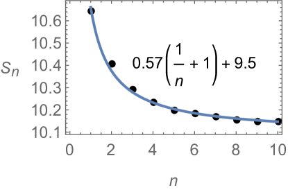
Figure 7: Renyi entropy $S_{n}$ as a function of $n$, denoted by black dots and fitted by blue line.

Our strategy is applicable to other tensor constraints constructed by tensor chains.

$\kappa_{c}=1$.

The tensor network with single constraint is plotted in Fig. 9. Irrespective of the interval $A$ one picks out on the boundary, no tensor is absorbed by the greedy algorithm. The CP tensor chain is closed and we always obtain a non-flat ES. On the other hand, wherever an operator is inserted in the bulk, it can not be pushed to the boundary with the use of the isometry. So such a tensor network does not enjoy QEC.

$\kappa_{c}=5/3$.

The tensor network with the constraint composed of three $T$ tensors is plotted in Fig. 9. Given an interval $A$ on the boundary, an operator inserted in the wedge of $A$ can be pushed to $A$. So such a tensor network enjoys QEC. While, it is subtle to justify whether the ES is flat or not. We find both flat and non-flat ES can be obtained, which depends on the specific choice of the interval $A$, as shown in Fig. 9. So we call this tensor network has a mixed ES.

The constructions of tensors $T$ and $E$ in above two tensor networks are given in Appendix A.

We list the properties of entanglement for above tensor networks with $\left\{5,4\right\}$ tiling in ordering of their $\kappa_{c}$ in Table. 1. We find that the higher $\kappa_{c}$ is, the stronger is the ability of QEC, but the ES more easily becomes flat. We remark that such a relation still holds in general cases. A detailed analysis on tensor networks with general tiling and general constraints is given in Ling:2018ajv , where the tensor networks with general constraints in terms of tensor chains are classified based on their properties of QEC and ES, with the power of CP reduced interior angle $\kappa_{c}$. The four tensor networks considered in this paper are typical examples of their own class.

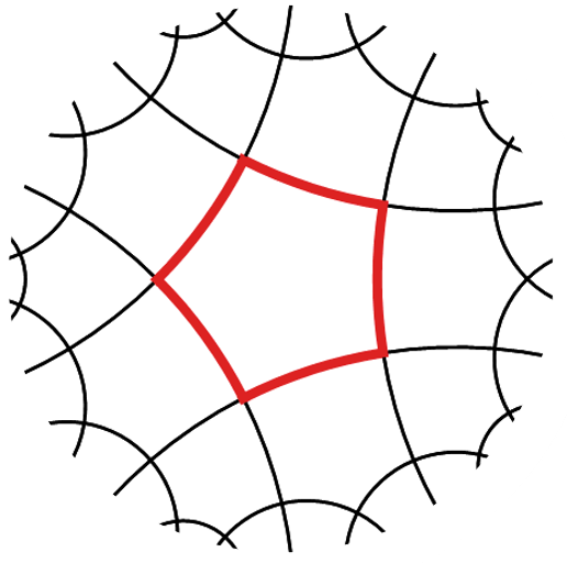
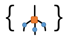
Figure 8: A tensor network with $\{5,4\}$ tiling and its tensor constraint. $\kappa_{c}=1/1=1$.

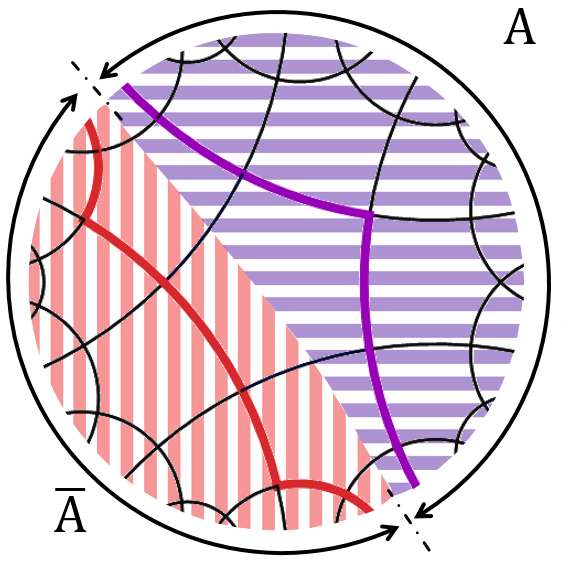
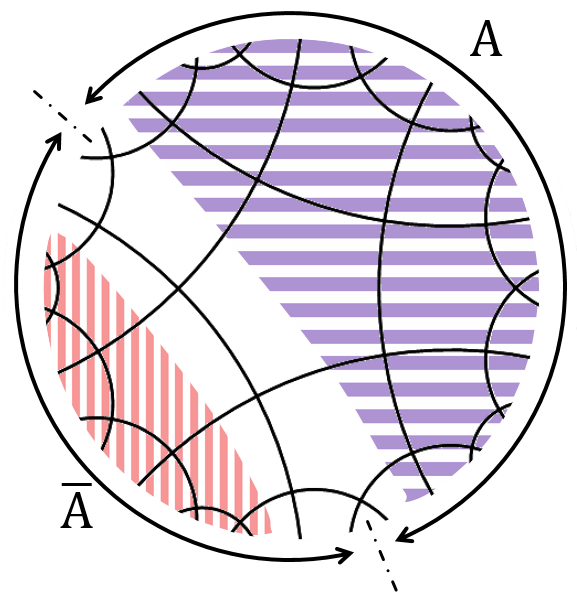
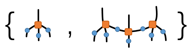
Figure 9: A tensor network with $\{5,4\}$ tiling and its tensor constraints. $\kappa_{c}=(1+2+2)/3=5/3$. Under the greedy algorithm, whether all the tensors are absorbed or not depends on the choice of $A$ and $\bar{A}$.

$\kappa_{c}$	1	3/2	5/3	2
QEC	N	Y	Y	Y
ES	non-flat	non-flat	mixed	flat

Table 1: The entanglement properties of tensor networks.

V Correlation function

Taking the tensor network with constraint (7) as an example, we show that the two-point correlation function in CFT can be reproduced here.

Given a local operator $O$ on the boundary, we may calculate the two-point correlation function

$$C(x_{1},x_{2})$$

$$= \frac{\left\langle\Psi\right|O(x_{1})O(x_{2})\left|\Psi\right\rangle}{Z}-\frac{\left\langle\Psi\right|O(x_{1})\left|\Psi\right\rangle\left\langle\Psi\right|O(x_{2})\left|\Psi\right\rangle}{Z^{2}}.$$

During the course of evaluating $\left\langle\Psi\right|O(x_{1})\left|\Psi\right\rangle$ ($\left\langle\Psi\right|O(x_{2})\left|\Psi\right\rangle$), all of the indexes are contracted except the indexes located at $x_{1}$ ($x_{2}$). It turns out that except those tensors in the neighborhood of $x_{1}$ ($x_{2}$), most of other tensors are absorbed by the greedy algorithm.

In $\left\langle\Psi\right|O(x_{1})O(x_{2})\left|\Psi\right\rangle$, all the indexes are contracted except the indexes located at $x_{1}$ and $x_{2}$. The greedy algorithm functions similarly as the case when we discuss QEC and ES. Let us consider $x_{1}$ and $x_{2}$ as those marked points in Fig. 6, then the tensors which are not absorbed by the greedy algorithm are just illustrated as in Fig. 6. As a result, the survived tensors $T$ and $E$ in $\left\langle\Psi\right|O(x_{1})O(x_{2})\left|\Psi\right\rangle$ form a bracket of matrix product state (MPS) sandwiching $O(x_{1})O(x_{2})$, as shown in Fig.10.

Furthermore, the MPS is formed by the tensors along the geodesic connecting $x_{1}$ and $x_{2}$. The length of the geodesic is proportional to the number of tensor pairs $TT^{\dagger}$ in Fig.10, i.e. the number of sites of the MPS, which is denoted as $l(x_{1},x_{2})$. Because of the tiling of $H^{2}$ space, when two points are far from each other, we have

$$l(x_{1},x_{2})=c\log|x_{1}-x_{2}|,$$ (20)

where $|x_{1}-x_{2}|$ is the number of the indexes between $x_{1}$ and $x_{2}$ on the boundary and $c$ is a constant based on the tiling.

Based on the interpretation of MPS, when $|x_{1}-x_{2}|$ is large enough, we can expect that the correlation function behaves like

$$C(x_{1},x_{2})\sim e^{-ml(x_{1},x_{2})}=|x_{1}-x_{2}|^{-mc},$$ (21)

where the positive coefficient $m$ reflects the gap of the theory describing the MPS. Our interpretation from MPS shares the same strategy with the one from bulk field dynamics in Susskind:1998dq . After all, (21) agrees with the result in CFT.

With the specific construction of tensors $T$ and $E$ in Appendix A, one can derive $C(x_{1},x_{2})$ concretely. In Appendix B, by adopting the construction in Fig. 19, we show that $C(x_{1},x_{2})$ satisfies (21) indeed. Especially, $m$ is determined by the inner construction of tensor $T$ and $E$ as well as the type of the operator $O$.

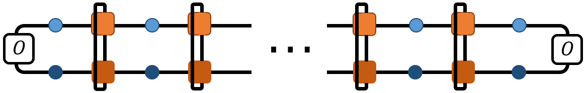
Figure 10: Those tensors which are not absorbed by the greedy algorithm in $\left\langle\Psi\right|O(x_{1})O(x_{2})\left|\Psi\right\rangle$ form a bracket of MPS, where each $TT^{\dagger}$ pair denotes a site.

Similarly, those higher-point functions can be evaluated in tensor networks as well. The network structure of three-point function is simplified under the action of the greedy algorithm into a MPS-like form: three linear MPSs are connected at a point in the bulk $y$, as shown in Fig. 12. The three-point correlation $C(x_{1},x_{2},x_{3})$, characterized by the connected part of $\left\langle\Psi\right|O(x_{1})O(x_{2})O(x_{3})\left|\Psi\right\rangle$, is supported by the two-point correlations of MPS between $\left\{x_{i},y\right\}$ for $i=1,2,3$ in the bulk. Thus,

$$\begin{split}&C(x_{1},x_{2},x_{3})\\ \sim&\exp\left\{-m\left[l(x_{1},y)+l(x_{2},y)+l(x_{3},y)\right]\right\}\\ \sim&\exp\left\{-\frac{1}{2}m\left[l(x_{1},x_{2})+l(x_{2},x_{3})+l(x_{3},x_{1})\right]\right\}\\ =&\left(|x_{1}-x_{2}||x_{2}-x_{3}||x_{3}-x_{1}|\right)^{-mc/2},\end{split}$$ (22)

where (20) is applied at the last step. (22) agrees with the result in CFT as well. Nevertheless, the network structure of four-point function can not be simplified into a MPS-like form any more, as shown in Fig. 12. A block of tensors in the bulk prevents a geometrical estimation of correlation. It also agrees with the fact that conformal symmetry can not fully determine the form of four-point function in CFT.

Above analysis can be applied to other tensor networks. The greedy algorithm plays a similar role as in the evaluation of ES, except that the boundary effect will be suppressed by the insertion of operators on the boundary.

Multi-point correlation functions in tensor networks can be reduced into some brackets of MPS. For a general tensor network, the generated MPS may have multiple layers. The number of layers is approximately proportional to the distance between two CP tensor chains beside the geodesic. It is interesting to notice that given a tiling of tensor network, this distance becomes larger with the increase of $\kappa_{c}$, which is observed if we compare different tensor networks in this paper with each other and is proved in Ling:2018ajv . Such tendency implies that the correlation between two endpoints carried by the MPS becomes stronger as well.

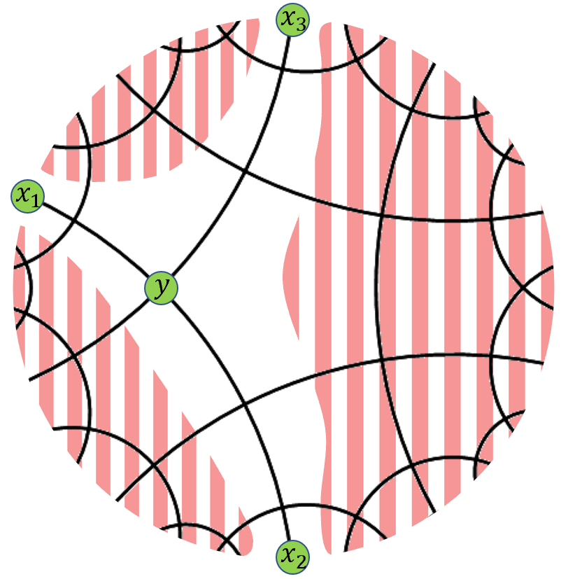
Figure 11: Three-point function.

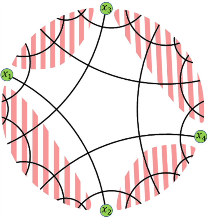
Figure 12: Four-point function.

VI Conclusion and Outlook

In this paper the notion of critical protection based on tensor chain has been proposed to describe the behavior of tensor networks under the action of greedy algorithm. In particular, a criteria has been developed with the help of the average reduced interior angle of CP chain such that for a given tensor network the ability of QEC and the flatness of ES can be justified in a quantitative manner. Currently it is still challenging to construct tensor networks which could capture all the holographic features of AdS spacetime. What we have found in this paper has shed light on this issue. Firstly, we have learned that the notion of critical protection provides a description on the limit of information transmission with full fidelity. CP tensor chain is the maximal boundary which can holographically store the interior information Flammia:2016xvs ; Jacobson:2015hqa . Thus, for a tensor network which is desired to capture the feature of QEC as AdS space, it must not contain circular CP curves. As a result, the tensor network with $\kappa_{c}=1$ in this paper is not a candidate of holography. Furthermore, among the examples of tensor networks considered in this paper, the tensor network with $\kappa_{c}=3/2$ has more likelihood to mimic the AdS holography since it exhibits both features of QEC and non-flat ES, which motivates us to propose some strategy to construct tensor networks in more general setup which could capture the desirable holographic aspects of AdS space, which will be explored in Ling:2018ajv .

The correlation in tensor networks with constraints becomes more transparent since the greedy algorithm reduces the structure of network into MPS lying on the geodesic. The number of layers in MPS is determined by CP tensor chains. This fact can be understood as the realization of Witten diagram in AdS space. Furthermore, from the viewpoint of field theory in bulk, the correlation function is the partition function of a particle in AdS space. Since the classical trajectory of the particle is just the geodesic, the partition function has the same form as (21), where $m$ is the mass of the particle. Therefore, we expect that the MPS may effectively describe the trajectory of a particle in AdS space, where the number of layers in MPS corresponds to the quantum fluctuations of the trajectory near the geodesic.

The geometric description of CP tensor chain is appealing. In the light of its periodic structure, we find the analogy of CP tensor chain is the curve of constant curvature in $H^{2}$ space such that $\kappa_{c}$ is related to the geodesic curvature of the curve Ling:2018ajv . Specifically, an open CP tensor chain corresponds to a hypercircle, which has a constant distance from its axes (a geodesic), as illustrated in Fig. 6. Such a distance measures the deviation from RT formula when evaluating the Renyi entropy, which may be linked to the tension of cosmic brane in Dong:2016fnf .

Because of the chain structure of tensor constraint, in our present framework we have investigated QEC and ES only for a single interval on the boundary. It is an open question whether these properties of entanglement can be realized for multi-intervals on the boundary, as investigated in network with perfect tensors or random tensors Hayden:2016cfa ; Yang:2015uoa ; Pastawski:2015qua .

Finally, beyond the applications in holography, we expect that tensor network models in this paper may be applicable to describe the quantum states of critical system in condensed matter physics as well, because of the $SL(2,R)$ symmetry in $H^{2}$ space. Imposing tensor constraints in terms of tensor chains leads to a generalized greedy algorithm, which is completely under control and would greatly simplify the calculation involved in tensor networks. The correlation and entanglement of the tensor network state will be determined by the tiling style, the tensor constraints ($\kappa_{c}$) as well as the specific construction of elementary tensors.

We are grateful to Long Cheng, Glen Evenbly, Wencong Gan, Muxin Han, Ling-Yan Hung, Shao-Kai Jian, Hai Lin, Wei Li, Fuwen Shu, Yu Tian, Menghe Wu, Xiaoning Wu and Hongbao Zhang for helpful discussions and correspondence. This work is supported by the NSFC under Grant No. 11575195. Y.L. also acknowledges the support from Jiangxi young scientists (JingGang Star) program and 555 talent project of Jiangxi Province. Z.Y.X. is supported by National Postdoctoral Program for Innovative Talents BX20180318.

Appendix A Specific Construction of Tensors Subject to Tensor Constraints

In Fig.15, 15 and 15, we define tensor $U$, tensor $Q$ and tensor $R$ as the building blocks for $T$ and $E$. The elements of tensor $U$ are $U_{\mu\nu}$. They satisfy following relations

$$\begin{split}U_{\mu\nu}=U_{\nu\mu},\\ \sum_{\nu}U_{\mu\nu}U_{\rho\nu}^{*}\propto\delta_{\mu\rho}.\end{split}$$ (23)

The elements of tensor $Q$ are $Q_{\mu\nu\rho\sigma}$ where two indexes $\mu\nu$ ($\rho\sigma$) are grouped together. They satisfy

$$\begin{split}Q_{\mu\nu\rho\sigma}=Q_{\rho\sigma\mu\nu}=Q_{\nu\mu\sigma\rho},\\ \sum_{\rho\sigma}Q_{\mu\nu\rho\sigma}Q_{\mu^{\prime}\nu^{\prime}\rho\sigma}^{*}\propto\delta_{\mu\mu^{\prime}}\delta_{\nu\nu^{\prime}}.\end{split}$$ (24)

The elements of tensor $R$ are $R_{\mu\nu\rho\sigma}$. They satisfy

$$\begin{split}R_{\mu\nu\rho\sigma}=R_{\rho\sigma\mu\nu}=R_{\nu\mu\sigma\rho},\\ \sum_{\rho\sigma}R_{\mu\nu\rho\sigma}R_{\mu^{\prime}\nu^{\prime}\rho\sigma}^{*}\propto\delta_{\mu\mu^{\prime}}\delta_{\nu\nu^{\prime}},\\ \sum_{\nu\sigma}R_{\mu\nu\rho\sigma}R_{\mu^{\prime}\nu\rho^{\prime}\sigma}^{*}\propto\delta_{\mu\mu^{\prime}}\delta_{\rho\rho^{\prime}}.\end{split}$$ (25)

Specifically, we construct the tensor $T$ and tensor $E$ for the tensor network with $\left\{5,4\right\}$ tiling for different tensor constraints, as shown in Fig.19,19,19 and 19. Specific elements of some tensors $Q$ and $R$ are given in Evenbly:2017htn .

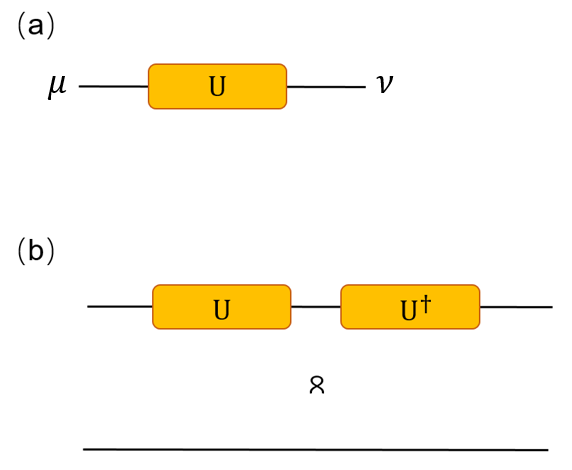
Figure 13: (a) Tensor $U$. (b) Tensor $U$ is proportional to an isometry.

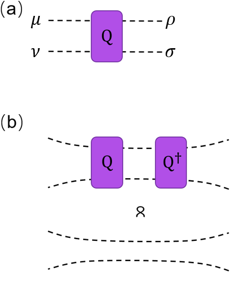
Figure 14: (a) Tensor $Q$, where two indexes on each side are grouped together. (b) Tensor $Q$ is proportional to an isometry between two grouped indexes.

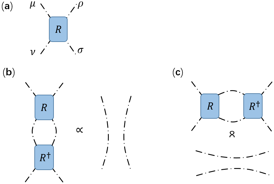
Figure 15: (a) Tensor $R$. (b) Tensor $R$ is proportional to isometries along two directions.

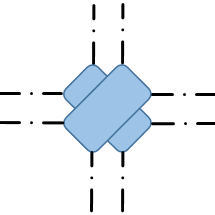
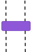
Figure 16: (a) Tensor $T$ and
(b) tensor $E$ in (4) and Fig.6.

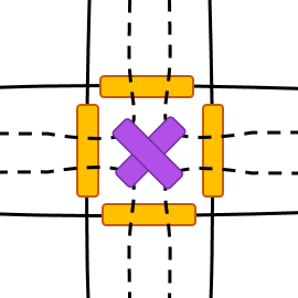
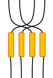
Figure 17: (a) Tensor $T$ and
(b) tensor $E$ in (7) and Fig.6.

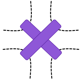
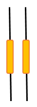
Figure 18: (a) Tensor $T$ and
(b) tensor $E$ in Fig.9).

Figure 19: (a) Tensor $T$ and
(b) tensor $E$ in Fig.9).

Appendix B Correlation Function in a Specific Tensor Network

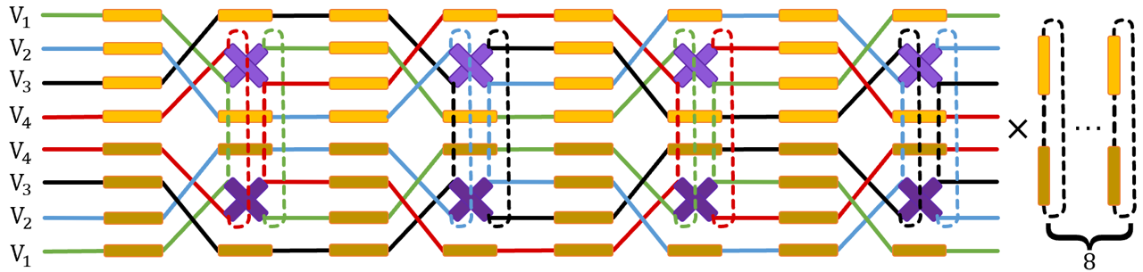
Figure 20: The inner structure of $V$, a part of $\tilde{\rho}$ containing $4$ sites. $V$ is an outer product of $4$ channels $\left\{V_{1},V_{2},V_{3},V_{4}\right\}$.

Given a tensor network, we define the unnormalized reduced density matrix of two points $\left\{x_{1},x_{2}\right\}$ on the boundary as

$$\tilde{\rho}=\mathrm{Tr}_{\complement\left\{x_{1},x_{2}\right\}}\left|\Psi\right\rangle\left\langle\Psi\right|,$$ (26)

where $\complement\left\{x_{1},x_{2}\right\}$ is the supplementary of two points $\left\{x_{1},x_{2}\right\}$. Now we treat $\tilde{\rho}$ as a matrix with column index in $\mathcal{H}_{x_{1}}\otimes\mathcal{H}_{x_{1}}^{*}$ and row index in $\mathcal{H}_{x_{2}}\otimes\mathcal{H}_{x_{2}}^{*}$, where superscript “$*$” refers to the dual space. Meanwhile, operator $O$ is treated as a column vector. Then all the brackets in (V) can be expressed in terms of matrix product, such as $\left\langle\Psi\right|O(x_{1})O^{\prime}(x_{2})\left|\Psi\right\rangle=O^{T}\tilde{\rho}O^{\prime}$. Thanks to greedy algorithm, $\tilde{\rho}$ has a form of MPS, as shown in Fig. 10. One can show that $\tilde{\rho}$ is a symmetric matrix. Those tensors absorbed by the greedy algorithm contribute to $\tilde{\rho}$ as a constant factor but do not affect the correlation function, so we just set it to be $1$.

Adopting the specific construction of tensors in Fig. 19, we demonstrate one part of the inner structure of $\tilde{\rho}$ in Fig. 20, which plays a key role in the evaluation of the reduced density matrix. We observe that such a network which looks complicated is actually an outer product of $4$ individual networks and each of them has a period composed of $4$ sites, where each site is denoted by a pair of tensors $TT^{\dagger}$. We write $l(x_{1},x_{2})$ as $l$ for short. Since we are interested in the behavior of correlation function at large scale, it is enough to consider $l/4\in\mathbb{Z}$. Then $\tilde{\rho}$ can be decomposed into

$$\tilde{\rho}=V^{l/4}F,\quad V=\bigotimes_{i=1}^{4}V_{i},\quad F=E\otimes E^{\dagger}.$$ (27)

Four $V_{i}$’s have been marked out with different colors in Fig. 20. Actually, $\left\{V_{2},V_{3},V_{4}\right\}$ can be obtained by cycling $V_{1}$. So they share the same eigenvalues.

To evaluate these eigenvalues explicitly, we set $U$ and $Q$ to be

$$U_{\mu\nu}=\delta_{\mu\nu},\quad Q_{\mu\nu\rho\sigma}=\sqrt{1-r^{2}}\delta_{\mu\rho}\delta_{\nu\sigma}+ir\delta_{\mu\sigma}\delta_{\nu\rho},$$ (28)

where $\mu,\nu,\rho,\sigma=1,2,\cdots,d$ and $0<r<1$. The case of $r=0,1$ should be excluded, since it leads to the flatness of ES. Plugging it into $V_{1}$, we have

$$(V_{1})_{\mu\nu\rho\sigma}=d^{3}(1-r^{4})\delta_{\mu\nu}\delta_{\rho\sigma}+d^{4}r^{4}\delta_{\mu\rho}\delta_{\nu\sigma},$$ (29)

which is real and symmetric. It can be diagonalized as

$$V_{1} \to d^{4}\text{~{}diag}\left\{1,\underbrace{r^{4},r^{4},\cdots,r^{4}}_{d^{2}-1}\right\},$$ (30)

where the eigenvector of the eigenvalue $d^{4}$ is $\delta_{\mu\nu}$. We can further diagonalize $V$ as

$$V \to \bigotimes^{4}V_{1}$$ (32)

$$\to d^{16}\text{~{}diag}\left\{1,\underbrace{r^{4},\cdots,r^{4}}_{4(d^{2}-1)},\underbrace{r^{8},\cdots,r^{8}}_{6(d^{2}-1)^{2}},\right.$$

$$\left.\underbrace{r^{12},\cdots,r^{12}}_{4(d^{2}-1)^{3}},\underbrace{r^{16},\cdots,r^{16}}_{(d^{2}-1)^{4}}\right\}.$$

The first eigenvector is the identity operator $I$. We use $\alpha=0,1,2,3,4$ to label the degenerate subspace of eigenvalue $d^{16}r^{4\alpha}$. Since $\tilde{\rho}$ and $F$ are symmetric, from (27), we have

$$VF=FV^{T}.$$ (33)

So $F$ is diagonal between different subspaces.

We decompose the operator $O$ according to these five subspaces

$$O=\sum_{\alpha=0}^{4}O_{\alpha},\quad O_{\alpha}V=VO_{\alpha}=d^{16}r^{4\alpha}O_{\alpha}.$$ (34)

We find that

$$I^{T}FI = d^{4},$$ (35)

$$O_{\alpha}^{T}FI=I^{T}FO_{\alpha} = g\delta_{\alpha 0},$$ (36)

$$O_{\alpha}^{T}FO_{\alpha^{\prime}} = f_{\alpha}\delta_{\alpha\alpha^{\prime}},$$ (37)

where coefficients

$$f_{\alpha}=O_{\alpha}^{T}FO_{\alpha},\quad g^{2}=f_{0}d^{4}.$$ (38)

Now those brackets in (V) can be evaluated.

$$Z= I^{T}\tilde{\rho}I= d^{4l+4},$$ (39)

$$\left\langle\Psi\right|O(x_{1})\left|\Psi\right\rangle= O^{T}\tilde{\rho}I= d^{4l}g,$$ (40)

$$\left\langle\Psi\right|O(x_{2})\left|\Psi\right\rangle= I^{T}\tilde{\rho}O= d^{4l}g,$$ (41)

$$\left\langle\Psi\right|O(x_{1})O(x_{2})\left|\Psi\right\rangle= O^{T}\tilde{\rho}O= \sum_{\alpha=0}^{4}d^{4l}r^{\alpha l}f_{\alpha}.$$ (42)

Finally,

$$C(x_{1},x_{2}) = \frac{\sum_{\alpha}d^{4l}r^{\alpha l}f_{\alpha}}{d^{4l+4}}-\left(\frac{d^{4l}g}{d^{4l+4}}\right)^{2}$$ (43)

$$= \sum_{\alpha=1}^{4}f_{\alpha}d^{-4}r^{\alpha l}$$ (44)

$$= \sum_{\alpha=1}^{4}f_{\alpha}d^{-4}e^{-(\alpha\log\frac{1}{r})l}$$ (45)

which behaves like (21) with $m=\alpha\log\frac{1}{r}>0$ for the minimal $\alpha$ such that $f_{\alpha}\neq 0$.

References

- (1) J. M. Maldacena, “Eternal black holes in anti-de Sitter,” JHEP 0304, 021 (2003) [hep-th/0106112].
- (2) M. Van Raamsdonk, “Building up spacetime with quantum entanglement,” Gen. Rel. Grav. 42, 2323 (2010) [Int. J. Mod. Phys. D 19, 2429 (2010)] [arXiv:1005.3035 [hep-th]].
- (3) S. Ryu and T. Takayanagi, “Holographic derivation of entanglement entropy from AdS/CFT,” Phys. Rev. Lett. 96, 181602 (2006) [hep-th/0603001].
- (4) X. Dong, “The Gravity Dual of Renyi Entropy,” Nature Commun. 7, 12472 (2016) [arXiv:1601.06788 [hep-th]].
- (5) P. Calabrese and J. L. Cardy, “Entanglement entropy and quantum field theory,” J. Stat. Mech. 0406, P06002 (2004) [hep-th/0405152].
- (6) P. Calabrese and J. Cardy, “Entanglement entropy and conformal field theory,” J. Phys. A 42, 504005 (2009) [arXiv:0905.4013 [cond-mat.stat-mech]].
- (7) A. Hamilton, D. N. Kabat, G. Lifschytz and D. A. Lowe, “Holographic representation of local bulk operators,” Phys. Rev. D 74, 066009 (2006) [hep-th/0606141].
- (8) A. Almheiri, X. Dong and D. Harlow, “Bulk Locality and Quantum Error Correction in AdS/CFT,” JHEP 1504, 163 (2015) [arXiv:1411.7041 [hep-th]].
- (9) E. Mintun, J. Polchinski and V. Rosenhaus, “Bulk-Boundary Duality, Gauge Invariance, and Quantum Error Corrections,” Phys. Rev. Lett. 115, no. 15, 151601 (2015) [arXiv:1501.06577 [hep-th]].
- (10) X. Dong, D. Harlow and A. C. Wall, “Reconstruction of Bulk Operators within the Entanglement Wedge in Gauge-Gravity Duality,” Phys. Rev. Lett. 117, no. 2, 021601 (2016) [arXiv:1601.05416 [hep-th]].
- (11) B. Freivogel, R. Jefferson and L. Kabir, “Precursors, Gauge Invariance, and Quantum Error Correction in AdS/CFT,” JHEP 1604, 119 (2016) [arXiv:1602.04811 [hep-th]].
- (12) J. Cotler, P. Hayden, G. Salton, B. Swingle and M. Walter, “Entanglement Wedge Reconstruction via Universal Recovery Channels,” arXiv:1704.05839 [hep-th].
- (13) D. Harlow, “TASI Lectures on the Emergence of the Bulk in AdS/CFT,” arXiv:1802.01040 [hep-th].
- (14) B. Schumacher and M. A. Nielsen, “Quantum data processing and error correction,” Phys. Rev. A 54, 2629 (1996) [quant-ph/9604022].
- (15) F. Pastawski, B. Yoshida, D. Harlow and J. Preskill, “Holographic quantum error-correcting codes: Toy models for the bulk/boundary correspondence,” JHEP 1506, 149 (2015) [arXiv:1503.06237 [hep-th]].
- (16) D. Harlow, “The Ryu-Takayanagi Formula from Quantum Error Correction,” Commun. Math. Phys. 354, no. 3, 865 (2017) [arXiv:1607.03901 [hep-th]].
- (17) G. Vidal, “Entanglement Renormalization,” Phys. Rev. Lett. 99, no. 22, 220405 (2007) [cond-mat/0512165].
- (18) B. Swingle, “Entanglement Renormalization and Holography,” Phys. Rev. D 86, 065007 (2012) [arXiv:0905.1317 [cond-mat.str-el]].
- (19) B. Swingle, “Constructing holographic spacetimes using entanglement renormalization,” arXiv:1209.3304 [hep-th].
- (20) M. Nozaki, S. Ryu and T. Takayanagi, “Holographic Geometry of Entanglement Renormalization in Quantum Field Theories,” JHEP 1210, 193 (2012) [arXiv:1208.3469 [hep-th]].
- (21) X. L. Qi, “Exact holographic mapping and emergent space-time geometry,” arXiv:1309.6282 [hep-th].
- (22) I. H. Kim and M. J. Kastoryano, “Entanglement renormalization, quantum error correction, and bulk causality,” JHEP 1704, 040 (2017) [arXiv:1701.00050 [quant-ph]].
- (23) N. Bao, C. J. Cao, S. M. Carroll, A. Chatwin-Davies, N. Hunter-Jones, J. Pollack and G. N. Remmen, “Consistency conditions for an AdS multiscale entanglement renormalization ansatz correspondence,” Phys. Rev. D 91, no. 12, 125036 (2015) [arXiv:1504.06632 [hep-th]].
- (24) Z. Yang, P. Hayden and X. L. Qi, “Bidirectional holographic codes and sub-AdS locality,” JHEP 1601, 175 (2016) [arXiv:1510.03784 [hep-th]].
- (25) W. Donnelly, B. Michel, D. Marolf and J. Wien, “Living on the Edge: A Toy Model for Holographic Reconstruction of Algebras with Centers,” JHEP 1704, 093 (2017) [arXiv:1611.05841 [hep-th]].
- (26) A. Bhattacharyya, Z. S. Gao, L. Y. Hung and S. N. Liu, “Exploring the Tensor Networks/AdS Correspondence,” JHEP 1608, 086 (2016) [arXiv:1606.00621 [hep-th]].
- (27) G. Evenbly, “Hyper-invariant tensor networks and holography,” Phys. Rev. Lett. 119, 141602 [arXiv:1704.04229 [cond-mat, physics:quant-ph]].
- (28) P. Hayden, S. Nezami, X. L. Qi, N. Thomas, M. Walter and Z. Yang, “Holographic duality from random tensor networks,” JHEP 1611, 009 (2016) [arXiv:1601.01694 [hep-th]].
- (29) X. L. Qi and Z. Yang, “Space-time random tensor networks and holographic duality,” arXiv:1801.05289 [hep-th].
- (30) M. Han and L. Y. Hung, “Loop Quantum Gravity, Exact Holographic Mapping, and Holographic Entanglement Entropy,” Phys. Rev. D 95, no. 2, 024011 (2017) [arXiv:1610.02134 [hep-th]].
- (31) G. Chirco, D. Oriti and M. Zhang, “Ryu-Takayanagi Formula for Symmetric Random Tensor Networks,” arXiv:1711.09941 [hep-th].
- (32) M. Han and S. Huang, “Discrete gravity on random tensor network and holographic Renyi entropy,” JHEP 1711, 148 (2017) [arXiv:1705.01964 [hep-th]].
- (33) B. Schumacher, and M. D. Westmoreland, “Approximate Quantum Error Correction,” Quantum Information Processing 1, 5–12 (2002) [arXiv:quant-ph/0112106].
- (34) Y. Ling, Y. Liu, Z. Y. Xian and Y. Xiao, “Tensor chain and constraints in tensor networks,” arXiv:1807.10247 [hep-th].
- (35) L. Susskind and E. Witten, “The Holographic bound in anti-de Sitter space,” hep-th/9805114.
- (36) S. T. Flammia, J. Haah, M. J. Kastoryano and I. H. Kim, “Limits on the storage of quantum information in a volume of space,” Quantum 1, 4 (2017) [arXiv:1610.06169 [quant-ph]].
- (37) T. Jacobson, “Entanglement Equilibrium and the Einstein Equation,” Phys. Rev. Lett. 116, no. 20, 201101 (2016) [arXiv:1505.04753 [gr-qc]].