Proactive Resource Allocation with Predictable Channel Statistics

Abstract

The behavior of users in relatively predictable, both in terms of the data they request and the wireless channels they observe. In this paper, we consider the statistics of such predictable patterns of the demand and channel jointly across multiple users, and develop a novel predictive resource allocation method. This method is shown to provide performance benefits over a reactive approach, which ignores these patterns and instead aims to satisfy the instantaneous demands, irrespective of cost to the system. In particular, we show that our proposed method is able to attain a novel fundamental bound on the achievable cost, as the service window grows. Through numerical evaluation, we gain insights into how different uncertainty sources affect the decisions and the cost.

I Introduction

With the increase in number of users and data traffic per users, come major challenges for network operators, leading to a need for more intelligence at the network side [2]. In the last decade, the predictability of users has been assessed, indicating that users are is not completely random in terms of their demand patterns [3, 4, 5] or in the wireless channel qualities they observe [6, 7, 8, 9]. This latter effect is a consequence of fixed mobility and behavioral patterns, as well as the characteristics of wireless propagation.

Unlike conventional scheduling, which operates at the millisecond time scale, predictability can be exploited for scheduling at a much slower time scale (seconds, minutes) [10, 11]. Networks currently assign resources to users at the slower time scale in a reactive manner, regardless of channel quality (e.g., by setting priority levels) [12]. Future networks on the other hand can collect data regarding users’ demand and mobility patterns, which can be combined with user predictability to forecast the user’s demand and channel. This leads to extra degrees of freedom to be exploited, by allocating resources ahead of time. The main advantage of this approach is network load balancing over large time scale dynamics, at the expense of possible waste of network resources [13].

Predictive resource optimization schemes for efficient video content streaming based on user channel quality metrics (CQM) are studied in [14, 15, 16, 17]. Under known demands, [18, 19] analyzed energy-efficient policies for scheduling with statistical CQM knowledge. In [6, 7, 8, 9], a location-aided framework was proposed and showed how large-scale channel characteristics of the wireless channel can be predicted by exploiting the user’s location information. Since location-aided predicted CQM is coarse, it can be efficiently harnessed in predictive/proactive resource allocation whereby demand dynamics and large-scale channel characteristics vary within the same time scale. These above works focus on channel predictability, ignoring the demand statistics. Demand statistics were considered in the following works. In [20, 21], user delay was evaluated under proactive scheduling and was found to be reduced the longer the prediction window. The predictable demands were exploited in [22, 13]: [22] proposed a proactive resource allocation framework, while [13] derived lower bounds on the cost of such proactive resource allocation with time-varying user demands, as well as policies that can asymptotically attain these bounds, again as the prediction window is increased. The joint treatment of channel predictability and user demand predictability is not considered in these works, which is the gap the current paper aims to address.

In this work, we study proactive resource allocation strategies that exploit both the predictable data demand and channel characteristics, with uncertainties. Our main focus will be on time-varying, but predictable channel statistics, as would be experienced when a user traverses a known path. The main contributions of this paper can be summarized as follows:

• We extend the work in [13, 1]: while [13] did not consider the effect of the channel, here it is included explicitly. Moreover, our preliminary study [1] focused on time-invariant channels, while we here explicitly consider the effect of time-varying channel statistics. In addition, we allow for general correlation among demands and among user statistics.

• We establish global lower bounds on the proactive scheduling cost that capture the impact of demand and channel uncertainties. Specifically, we compute lower bounds for two scenarios: (i) time-invariant demand and channel statistics, (ii) time-invariant demand and time-varying channel statistics.

• We develop asymptotically optimal service policies that can attain the bounds as the proactive service window grows in size.

• Through Monte Carlo simulations, we show the performance benefits of the proactive schedulers over a reactive scheduler, in terms of channel load and network cost.

The remainder of the paper is structured as follows. Section II presents the system model comprising user demand model, wireless channel model, and reactive and proactive network models. Section III provides empirical support for the key assumption related to the channel for the proactive network model. In Section IV, we present a global lower bound for both time-invariant and time-varying channel statistics, as well as asymptotically optimal stationary policies. Finally, numerical results are given in Section V, followed by the conclusions in Section VI.

Notation

Vectors and matrices are written in bold (e.g., a vector $\mathbf{k}$ and a matrix $\mathbf{K}$); $\mathbb{E}[.]$ denotes expectation; $[a_{n}]_{n=1}^{N}$ is a shorthand for $[a_{1},\ldots,a_{N}]^{T}$; $\delta_{n\in\mathcal{B}}=1$ when $n\in\mathcal{B}$ and zero otherwise.

II System Model

We consider a network system wherein the data requests from a set of users are serviced by the SP. The SP provides service to each user on per time slot basis considering the demand request from the users. We assume that the network consists of set of $N$ users $\mathcal{N}=\{1,2,\ldots n,\ldots,N$}. The time slots are indexed by $t$ and all time slots all of them have fixed duration. The users send data requests to the SP based on their data requirements. The data request generation from the user is capture by a binary random variable $d_{n,t}\in\{0,1\}$. When $d_{n,t}=1$, the user $n$ generates a data request in time slot $t$, and when $d_{n,t}=0$, there is no data request from user $n$. Demands may be correlated among users (e.g., based on their social connection). We consider a discrete random variable $g_{n,t}\in\mathbb{R}_{+}$ to capture the user experienced channel quality. The channel qualities may also be correlated among users (e.g., if they are in close proximity). The SP spends $S$ amount of resources for service each request from the user. The statistics of the random variables of $d_{n,t}$ and $g_{n,t}$, as well as the cost function to be minimized by SP are described below.

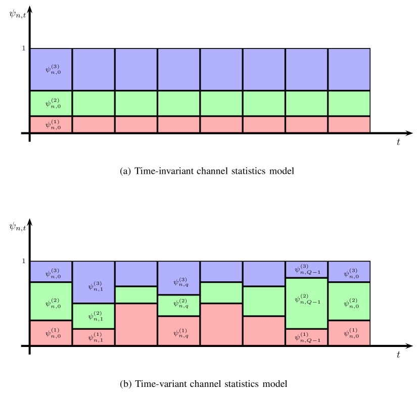
Figure 1: Channel statistics model: Inset (a) time-invariant channel statistics in which the channel state probabilities do not vary with time. Inset (b) time-varying channel statistics, wherein channels exhibit a cyclo-stationarity behavior with period $Q$.

II-A Demand and channel statistics

II-A1 User demand statistics

We assume that the current data request of each user is known to the SP. Furthermore, we consider a time-invariant demand statistics model, where the demand probabilities do not vary in each $t$. The time-invariant demand statistics model is of the form $\pi_{n,t}=p(d_{n,t}=1)$ for all times $t$. For simplicity of exposition, we will assume the statistics to be constant, with $d_{n,t}$ being i.i.d. with $\mathbb{E}[d_{n,t}]=\bar{\pi}_{n}$. We can capture demand profile of all the users in a set $\bar{\boldsymbol{\pi}}=\{\bar{\pi}_{1},\ldots,\bar{\pi}_{N}\}$ and is known to the SP. User demand requests cannot be delayed but can be serviced beforehand, which means the SP has to offer service to a request in time $t$ no later than at time $t$.

II-A2 Channel statistics

The channel gain experienced by user $n$ in time slot $t$ is denoted by $g_{n,t}$. As aforementioned, $g_{n,t}$ is modeled as discrete random variable with $K_{n}$ states. The $K_{n}$ states are from a finite set $\mathcal{C}_{n}=\{g_{n}^{(k)},\,k=1,\ldots,K_{n}$}. The statistics of $g_{n,t}$ are described by $\bm{\psi}_{n,t}=\{\psi_{n,t}^{(k)},k=1,\ldots,K_{n}\}$. The channel is considered to be cyclo-stationary, so that the $\bm{\psi}_{n,t}$ is periodic in $t$ with period $Q$, which is assumed to be the same for all users. Hence, the channel statistics of all users are determined by

$$\boldsymbol{\Psi}^{Q}=\left\{\mathcal{C}_{n},\bm{\psi}_{n,0},\ldots,\bm{\psi}_{n,Q-1}\right\}_{n=1}^{N}.$$

As a special case, when $Q=1$, the channel becomes time-invariant and is characterized by $\boldsymbol{\Psi}=\left\{\mathcal{C}_{n},\bm{\psi}_{n}\right\}_{n=1}^{N}.$ The difference between time-invariant and time-varying channel statistics model is shown in Fig. 1. The channel statistics are assumed to be known to SP. This can be accomplished, e.g., by building a database of the propagation environment combined with users sending their planned trajectory to the scheduler. This is further elaborated in Section III.

II-B Cost function

The load is a function of the amount of service $\mathsf{S}_{n}$ that is provided to a user $n$,

$$L_{n} =\mathsf{S}_{n}.$$ (1)

We can view $\mathsf{S}_{n}$, for example, as the total number of bits to be delivered. The cost to the SP for serving $N$ users, with vector of channels $\mathbf{g}=[g_{1},\ldots,g_{N}]^{T}$ is denoted by $C_{d}(\mathbf{L};\mathbf{g})$, where $C_{d}:(\mathbb{R}_{+}^{N},\mathbb{R}_{+}^{N})\rightarrow\mathbb{R}_{+}$, is strictly convex and increasing in $\mathbf{L}=[L_{1},\ldots,L_{N}]^{T}$, while being decreasing in $\mathbf{g}$ (since a better channel require less cost for a given load $\mathbf{L}$).

We study two network models, reactive and proactive, whose cost functions are further described below.

II-B1 Reactive network model

The reactive network model will be our baseline approach. In the reactive network model, the SP has to serve the user data requests upon their arrival. The amount of load user $n$ generates in time slot $t$ for a reactive network (1) can be computed as

$$L_{n,t}^{\mathcal{R}} =S\,d_{n,t}.$$ (2)

We can write for the reactive network, the time-averaged cost as

$$c^{\mathcal{R}}(\bar{\boldsymbol{\pi}},\boldsymbol{\Psi}^{Q})=\underset{t\rightarrow\infty}{\limsup}\frac{1}{t}\sum_{l=0}^{t-1}\,\mathbb{E}\biggl{[}C_{d}\Bigl{(}\mathbf{L}_{t}^{\mathcal{R}};\mathbf{g}_{t}\Bigr{)}\biggr{]},$$ (3)

where expectation is over the joint demand and joint channel statistics of the users, in which as before $\mathbf{L}_{t}^{\mathcal{R}}$ is the vector of loads and $\mathbf{g}_{t}=[g_{1,t},g_{2,t},\ldots,g_{N,t}]^{T},\,g_{n,t}\in\mathcal{C}_{n}$ is the vector of channels at time $t$.

II-B2 Proactive network model

Unlike reactive network, the proactive network possesses the flexibility in servicing the user data requests before their actual realization. Therefore, the SP utilizes the demand profile $\bar{\boldsymbol{\pi}}$ of the users in providing proactive serve for each request in $T$ time slots ahead, where $T$ denotes the proactive service window (see Fig. 2). The key factor that determines the choice of $T$ is content recency and availability, as users may consume content that is not older than $T$ slots. The SP knows the demand $\bar{\boldsymbol{\pi}}$ and channel $\boldsymbol{\Psi}^{Q}$ profile of the users, and therefore it tries to even out the load over the $T$ time-slot proactive service window. To this end, we denote by $u_{n,t}(\tau)$ the amount of proactive service applied to a user $n$ at time slot $t$ for a possible request, $\tau$ slots in the future, i.e., at time $t+\tau$, where $1\leq\tau\leq T$. The proactive service at times $t-\tau$ for a future request at time $t$ cannot exceed the total demand of $S$ units of service, i.e.,

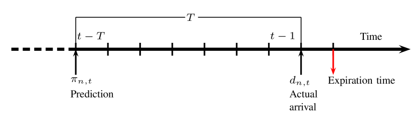
Figure 2: A user request $d_{n,t}$ is proactively served $T$ (proactive service window) slots ahead, where $\pi_{n,t}$ is the probability of request $d_{n,t}$ being realized at time $t$.

$$\sum_{\tau=1}^{T}u_{n,t-\tau}(\tau)\leq S$$ (4)

and the proactive service can never be negative, i.e.,

$$u_{n,t}(\tau)\geq 0.$$ (5)

With the total proactive service at time $t$ denoted by $\mathbf{u}_{n,t}=[u_{n,t}(1),\ldots,u_{n,t}(T)]$, the load of user $n$ is written as

$$L_{n,t}^{\mathcal{\mathcal{P}}}(\mathbf{u}_{n,t})=$$ (6)

$$(S-\sum_{\tau=1}^{T}u_{n,t-\tau}(\tau))d_{n,t}+\sum_{\tau=1}^{T}u_{n,t}(\tau).$$

In 6, the term $\sum_{\tau=1}^{T}u_{n,t-\tau}(\tau)$ denotes the amount of proactive services for user $n$ that was already applied earlier. Therefor in time slot $t$, the remaining data that has to be served by SP based on the user request is $S-\sum_{\tau=1}^{T}u_{n,t-\tau}(\tau)$. Finally, the term $\sum_{\tau=1}^{T}u_{n,t}(\tau)$ corresponds to the proactive service to be applied at time $t$ for user $n$ over the next $T$ slots, to be used in the future. The goal of the proactive controller is to determine the optimal online proactive service policy that minimizes the time averaged expected cost while delivering the content on time:

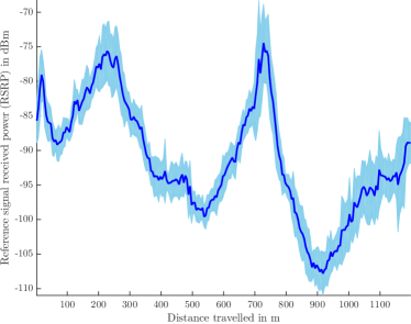
(a)

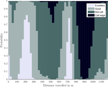
(b)

Figure 3: We have conducted channel measurement campaign using a smart phone, wherein we measured RSRP. Inset (a) a user is walking along a pedestrian path (Pilbågsgatan-Läraregatan). The solid line is the mean RSRP with measurements averaged over different times of the day and at different days. The shaded region captures the standard deviation of the measurements. Inset (b) depicts the channel state probabilities along the path.

$$\underset{\{u_{n,t}(\tau)\}_{n,t,\tau}}{\min} \underset{t\rightarrow\infty}{\limsup}\frac{1}{t}\sum_{t^{\prime}=0}^{t-1}\,\mathbb{E}\biggl{[}C_{d}\Bigl{(}\mathbf{L}_{t^{\prime}}^{\mathcal{P}}(\mathbf{u}_{t^{\prime}});\mathbf{g}_{t^{\prime}}\Bigr{)}\biggr{]}$$ (7)

s.t. $$(\ref{eq:proac_cont_const_1}),\,(\ref{eq:proac_cont_const_2}),$$

the optimal value of which is denoted by $c_{T}^{\mathcal{P}}(\bar{\boldsymbol{\pi}},\boldsymbol{\Psi}^{Q})$. Here we introduced $\mathbf{L}_{t^{\prime}}^{\mathcal{P}}$ as the vector of loads and $\mathbf{u}_{t^{\prime}}=[\mathbf{u}_{1,t^{\prime}}^{T},\ldots,\mathbf{u}_{N,t^{\prime}}^{T}]^{T}$. First, we will derive a global lower bound on the proactive scheduling cost (7) and then design an asymptotically optimal policy that achieves the lower bound. Note that the reactive model is recovered when $u_{n,t}(\tau)\equiv 0$.

III Channel Predictability

The aforementioned proactive model relies on the assumption that channel statistics can be predicted for an extended period of time. To validate this assumption, we have performed a measurement campaign using off-the-shelf hardware in Gothenburg, Sweden [2]. Similar findings have been reported in [9, 8, 23, 24, 25].

III-A Measurement set-up

The channel quality measurements were in the form of reference signal received power (RSRP), an important metric for measuring cell selection and handover. RSRP was collected by using a Google Nexus 5X smartphone and logged using GNet Track Pro by Gyokov solutions. The application allowed logging of signal strength, GPS position and many other parameters. Measurements along pre-specified paths were taken during various times of the day. These measurements were then mapped to a one dimensional space with the distance from a fixed point as one of the parameters. The starting and ending points are located at known fixed geographical positions, allowing the same track to be recorded several times. Three measurement campaigns were conducted: one walking on a street, one in a tram going through a tunnel, and one on a bus touring the city.

III-B Measurement findings

Fig. 3 (a) shows the RSRP values along the track for the walking path. We observe large variations of the RSRP, depending on the position. We also see that over the span of multiple days, the RSRP at a given position is relatively stable, with variations due to environmental factors as well as GPS errors. Peaks in the RSRP are due to direct line of sight connections with base stations, while valleys are due to shadowing by large buildings and other structures. In conclusion, the assumption of predictable received power appears to be reasonable, provided the path of the user along the proactive service window is known. The distributions from Fig. 1 can be related to Fig. 3 (b), where space is mapped into time slots and the RSRP values are quantized. The channel measurements in Fig. 3 (a) are categorized in four channel states namely, excellent ($\textrm{RSRP}\geq-80\,\textrm{dBm}$) , good ($-80\,\textrm{dBm}<\textrm{RSRP}\leq-90\,\textrm{dBm}$), mid cell ($-90\,\textrm{dBm}<\textrm{RSRP}\leq-100\,\textrm{dBm}$), and cell edge ($\textrm{RSRP}\leq-100\text{\,{dBm}}$). In Fig. 3 (b), we can clearly observe channel state probabilities varying with position. Depending on the velocity of the user, the channel state probabilities can be mapped to time. It is clear that the measurements follow the time-varying model in Fig. 1 (b), rather than the time-invariant model from Fig. 1 (a). We note that the corresponding average time-invariant probabilities are [0.11 0.32 0.41 0.16], from excellent to cell edge channel conditions.

IV Proactive Service with Future Channel Statistics

In this section, we aim to find solutions to (7), leading to proactive gains to flatten the load and cost. As the infinite horizon optimization of (7) is of infinite dimensionality, its exact solution is computationally intractable. We thus propose to tackle this problem through a two-step approach. First, we establish a fundamental lower bound on the minimum cost, then we develop an asymptotically optimal proactive caching strategy that achieves the lower bound as the proactive service window grows.

Given $\mathbf{g}_{t}$, a channel realization vector in time $t$, the probability of this vector being realized is $P_{c}(\mathbf{g}_{t})$.

IV-A Time-invariant channel statistics

We establish a global lower bound on the achievable costs by any proactive caching policy. We first introduce the following notation: $\mathcal{B}_{t}=\{n\in\mathcal{N}:\;d_{n,t}=1\}$ with probability $P_{d}(\mathcal{B})$, the set of requesting users at time $t$, and $P_{c}(\mathbf{g})$ the probability of an aggregate channel $\mathbf{g}=[g_{1},\ldots,g_{N}]$. As the channel statistics are time-invariant, therefore $P_{c}(\mathbf{g})$ does not depend on $t$ and can be easily derived from $\boldsymbol{\Psi}$.

Theorem 1.

The optimal time average expected cost $c_{T}^{\mathcal{P}}(\bar{\boldsymbol{\pi}},\boldsymbol{\Psi})$ satisfies

$$c_{T}^{\mathcal{P}}(\bar{\boldsymbol{\pi}},\boldsymbol{\Psi})\geq\underline{c}_{\mathcal{U}}(\bar{\boldsymbol{\pi}},\boldsymbol{\Psi}),$$ (8)

where $\underline{c}_{\mathcal{U}}(\bar{\boldsymbol{\pi}},\boldsymbol{\Psi})$ is the optimal value of

$$\min\Biggl{\{}\sum_{\mathbf{g}\in\mathcal{C}}\sum_{\mathcal{B}\subseteq\mathcal{N}}P_{c}(\mathbf{g})P_{d}(\mathcal{B})$$

$$C_{d}\Biggl{(}\left[(S-\bar{\mu}_{n})+\tilde{\mu}_{n}\left(\mathcal{B},\mathbf{g}\right)\right]_{n=1}^{N};\mathbf{g}\Biggr{)}\Biggr{\}}$$

subject to $$0\leq\tilde{\mu}_{n}\left(\mathcal{B},\mathcal{\mathbf{g}}\right)\leq S$$, (9)

where $\tilde{\mu}_{n}\left(\mathcal{B},\mathcal{\mathbf{g}}\right)$ are the optimization variables and $\bar{\mu}_{n}=\sum_{\mathbf{h}\in\mathcal{C}}\sum_{\mathcal{D}\subseteq\mathcal{N}}P_{c}(\mathbf{h})P_{d}(\mathcal{D})\,\tilde{\mu}_{n}\left(\mathcal{D},\mathcal{\mathbf{h}}\right)$.

Proof:

See Appendix A. ∎

Remark

In the objective of (9), the term $\bar{\mu}_{n}$ represents the average of the proactively cached content at user $n$ for an expected request. The term $\tilde{\mu}_{n}\left(\mathcal{B},\mathbf{g}\right)$ is the average of the total amount of proactively cached content at user $n$ in a time slot, when the set of requesting users is $\mathcal{B}$ and the respective channel gain is $\mathbf{g}$. Now, observing that the optimization problem of $\underline{c}_{\mathcal{U}}(\bar{\boldsymbol{\pi}},\boldsymbol{\Psi})$ is convex with closed and bounded constraints set, the optimization problem has a unique solution.

We now harness the established lower bound and the optimization (9), to develop our proposed asymptotically optimal stationary policy

Definition 2.

(Policy $\wp_{\mathcal{U}}$) Let $\{\tilde{\mu}_{n}\left(\mathcal{B},\mathcal{\mathbf{g}}\right)\}_{n,\mathcal{B},\mathbf{g}}$ be the optimal solution to (9). We consider the proactive scheduling policy $\wp_{\mathcal{U}}$ that in every time slot observes the set of requesting users $\mathcal{B}_{t}$, and channel gain realization $\mathbf{g}_{t}$, and then decides a proactive caching control $u_{n,t}(\tau)=\frac{1}{T}\tilde{\mu}_{n}\left(\mathcal{B}_{t},\mathcal{\mathbf{g}}_{t}\right)$, $\forall n,t,1\leq\tau\leq T$.

The policy $\wp_{\mathcal{U}}$ is determined offline, based on the demand $\bar{\boldsymbol{\pi}}$ and channel $\boldsymbol{\Psi}$ profiles. During online operation, the policy is a function of the current realization of demand and channel and requires a look-up table of length $2^{N}\prod_{n}|\mathcal{C}_{n}|$, which entails a search process of complexity $O(N+\sum_{n}\log(|\mathcal{C}_{n}|))$. Note that, to apply policy $\wp_{\mathcal{U}}$, the solution of (9) has to be obtained offline based on the demand $\bar{\boldsymbol{\pi}}$ and channel $\boldsymbol{\Psi}$ profiles. We can now establish the asymptotic optimality property of policy $\wp_{\mathcal{U}}$.

Theorem 3.

Denote the time average expected cost under policy $\wp_{\mathcal{U}}$ by $c_{T}^{\wp_{\mathcal{U}}}(\bar{\boldsymbol{\pi}},\boldsymbol{\Psi})$. Then policy $\wp_{\mathcal{U}}$ is asymptotically optimal, in the sense that

$$\limsup_{T\to\infty}|c_{T}^{\wp_{\mathcal{U}}}(\bar{\boldsymbol{\pi}},\boldsymbol{\Psi})-c_{T}^{\mathcal{P}}(\bar{\boldsymbol{\pi}},\boldsymbol{\Psi})|=0.$$

Proof:

See Appendix B. ∎

With the relevant characteristics of proactive caching for time-invariant channels have been investigated, we are ready to consider the scenario of of time-varying channel statistics.

IV-B Time-varying channel statistics

In this section, we follow a similar procedure, but for the case with time-varying channel statistics. Due to the cyclo-stationary nature of the channel, we introduce a new random variable, in order to develop a stationary policy. We denote by $s_{t}\in\mathcal{Q}=\{0,1,\ldots,Q-1\}$ the index in the period corresponding to time slot $t$, with $P_{\mathrm{s}}(s_{t})=1/Q$. The channel statistics can thus be interpreted as a function of $s$.

Theorem 4.

When $T$ is an integer multiple of $Q$, the minimum time average cost $c_{T}^{\mathcal{P}}(\bar{\boldsymbol{\pi}},\boldsymbol{\Psi})$ satisfies

$$c_{T}^{\mathcal{P}}(\bar{\boldsymbol{\pi}},\boldsymbol{\Psi}^{Q})\geq\underline{c}_{\mathcal{F}}(\bar{\boldsymbol{\pi}},\boldsymbol{\Psi}^{Q}),$$ (10)

where $\underline{c}_{\mathcal{F}}(\bar{\boldsymbol{\pi}},\boldsymbol{\Psi}^{Q})$ is the optimal value of

$$\min\Biggl{\{}\sum_{s\in\mathcal{Q}}P_{\mathrm{s}}(s)\sum_{\mathbf{g}\in\mathcal{C}}\,P_{c}(\mathbf{g}|s)\sum_{\mathcal{B}\subseteq\mathcal{N}}\,P_{d}(\mathcal{B})$$

$$\times C_{d}\biggl{(}\Bigl{[}\delta_{n\in\mathcal{B}}(S-\bar{\mu}_{n}(s))$$

$$+\sum_{s^{\prime}\in\mathcal{Q}}P_{\mathrm{s}}(s^{\prime})\tilde{\mu}_{n}\left(\mathcal{B},\mathbf{g},s,s^{\prime}\right)\Bigr{]}_{n=1}^{N};\mathbf{g}\biggr{)}\Biggr{\}}$$

$$\text{{}subject to $0\leq\tilde{\mu}_{n}\left(\mathcal{B},\mathbf{g},s,s^{\prime}\right)\leq S$},$$ (11)

where $\tilde{\mu}_{n}\left(\mathcal{B},\mathbf{g},s,s^{\prime}\right)$ are the optimization variables and

$$\bar{\mu}_{n}(s)=$$

$$\sum_{s^{\prime}\in\mathcal{Q}}P_{\mathrm{s}}(s^{\prime})\,\sum_{\mathbf{h}\in\mathcal{C}}P_{c}(\mathbf{h}|s^{\prime})\sum_{\mathcal{D}\subseteq\mathcal{N}}P_{d}(\mathcal{D})\,\tilde{\mu}_{n}\left(\mathcal{D},\mathcal{\mathbf{h}},s^{\prime},s\right).$$

Proof:

Please refer Appendix C. ∎

Remark

Similar to the optimization of $\underline{c}_{\mathcal{U}}(\bar{\boldsymbol{\pi}},\boldsymbol{\Psi})$, the optimization $\underline{c}_{\mathcal{F}}(\bar{\boldsymbol{\pi}},\boldsymbol{\Psi}^{Q})$ is also convex with a unique solution since the constraints set is compact and the objective function $C_{d}(.)$ is strictly convex. In the objective of (11) the term $\bar{\mu}_{n}(s)$ captures the average proactive service offered to the user $n$ before the actual demand request has arrived, when the current time slot corresponds to index $s$. Further, the term $\sum_{s^{\prime}\in\mathcal{Q}}P_{\mathrm{s}}(s^{\prime})\tilde{\mu}_{n}\left(\mathcal{B},\mathbf{g},s,s^{\prime}\right)$ captures the expected amount of content proactively served to user $n$, when the set of demanding users is $\mathcal{B}$, the current slot corresponds to index $s$, and the present channel realization is $\mathbf{g}$.

We now show an asymptotically optimal policy design that attains the lower bound (11).

Definition 5.

(Policy $\wp_{\mathcal{F}}$) Given the current set $\mathcal{B}_{t}$ of requesting users in a time slot $t$, channel gain realization $\mathbf{g}_{t}$, and the current index in the period $s_{t}$, then the proactive scheduler $\wp_{\mathcal{F}}$ assigns proactive controls as $u_{n,t}(\tau)=\frac{1}{T}\tilde{\mu}_{n}\left(\mathcal{B}_{t},\mathbf{g}_{t},s_{t},s_{t+\tau}\right),$ $\forall n,t,1\leq\tau\leq T$, where $\tilde{\mu}_{n}\left(\mathcal{B},\mathbf{g},s,s^{\prime}\right)$ denote the optimal solution to (11).

The proposed policy $\wp_{\mathcal{F}}$ requires a look-up table of length $2^{N}\prod_{n}|\mathcal{C}_{n}|\,|\mathcal{Q}|^{2}$, that matches each combination of a requesting set of users and channel gain realization with a proactive caching control. The complexity of searching such a look-up table is $O(N+\sum_{n}\log(|\mathcal{C}_{n}|)+2\,\log(|\mathcal{Q}|))$. In comparison to $\wp_{\mathcal{U}}$, the policy $\wp_{\mathcal{F}}$ takes in to consideration statistical information not only of the current channel probabilities (represented by $s_{t}$) but also the future set of channel probabilities through $s_{t+\tau},\tau=1,\ldots,T$. This will help scheduler to shift the loads to time slots where the probabilities of higher channel state values are higher in order to minimize the overall network cost.

Theorem 6.

Under the time-invariant demand and time-varying channel statistics model described by $\boldsymbol{\Psi}^{Q}$. The policy $\wp_{\mathcal{F}}$ is asymptotically optimal, in the sense that $\limsup_{T\to\infty}$ $|c_{T}^{\wp_{\mathcal{F}}}(\bar{\boldsymbol{\pi}},\boldsymbol{\Psi}^{Q})-$ $c_{T}^{\mathcal{P}}(\bar{\boldsymbol{\pi}},\boldsymbol{\Psi}^{Q})|$ $=0$, where $c_{T}^{\wp_{\mathcal{F}}}(\bar{\boldsymbol{\pi}},\boldsymbol{\Psi}^{Q})$ denotes the time average expected cost under policy $\wp_{\mathcal{F}}$.

Proof:

The proof is similar to that of Theorem 3, and omitted here. ∎

V Numerical Results and Discussion

We assume that the network scheduler is aware of the user demand $\bar{\boldsymbol{\pi}}$ and channel $\boldsymbol{\Psi}^{Q}$ profiles. The scheduler spends $S=1$ units of service for each request. We take the cost function for the demand to be of a simple polynomial form $C_{d}(\mathbf{L}_{t},\mathbf{g}_{t})=\sum_{n=1}^{N}L_{n,t}^{4}/g_{n,t}$. While this choice of cost function is arbitrary, it is meant merely to illustrate the behavior of the proactive scheduler. Since demands will always be satisfied, performance will be evaluated in terms of the expected cost and the expected load.

V-A Time-invariant demand and channel statistics

We assume each user $n$ observes one of the two possible channel states $\{g_{n}^{(1)},g_{n}^{(2)}\}$ with probabilities $\{\psi_{n}^{(1)},\psi_{n}^{(2)}=1-\psi_{n}^{(1)}\}$. We consider $g_{n}^{(2)}\geq g_{n}^{(1)}$, hence $g_{n}^{(2)}$ is termed the good channel state, while $g_{n}^{(1)}$ is the bad channel state. Furthermore, for convenience we assume same channel state values and corresponding channel probability values for all the users.

V-A1 Impact of demand and channel probabilities on the expected cost

In Fig. 4, we compare the expected cost achieved by proactive and reactive schemes under time-invariant demand and channel statistics model for a single user scenario. We can infer easily from the Fig. 4 that the proactive schemes always offer lower expected cost compared to the reactive scheme irrespective of any demand and channel probability setting $(\bar{\pi}_{1},\psi_{1}^{(1)})$. The main reason for higher expected cost for reactive scheme is that, the reactive scheme does not possess the flexibility to delay the service requests and it has to fulfill the demand requests whenever they are initiated from the user. On the other hand the proactive scheme offers flexibility in the scheduling strategy by exploiting the demand and channel statistics to minimize cost by load balancing. When the demand $\bar{\pi}_{1}$ and channel $\psi_{1}^{(1)}$ probabilities are increased, the expected cost offered by both reactive and proactive is also increased. The cost increases with increase in $\bar{\pi}_{1}$ due to the fact that the system is more loaded with incoming demand requests. The reason for the cost to increase with $\psi_{1}^{(1)}$ is as the user more often experiences a bad channel state $g_{1}^{(1)}$ than a good channel state $g_{1}^{(2)}$.

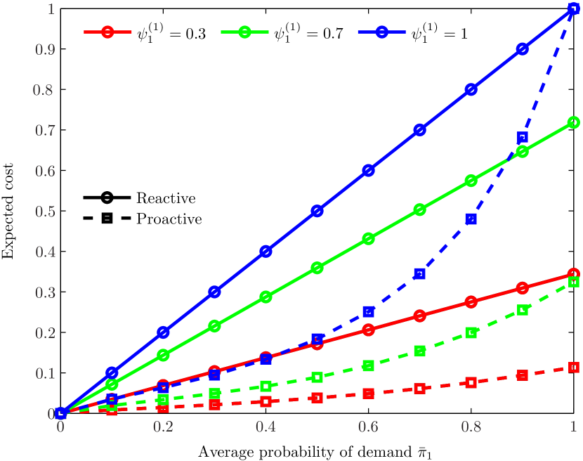
Figure 4: The expected cost for reactive and proactive schemes for single user scenario under the time-invariant demand and channel statistics model. The probabilities of the demand $\bar{\pi}_{1}$ and channel $\psi_{1}^{(1)}$ are varied with the channel states fixed to $g_{1}^{(1)}=1$ (bad channel state), $g_{1}^{(2)}=2$ (good channel state).

In [13], it was shown that both reactive and proactive schemes converge when $\bar{\pi}_{1}=1,$ under time-invariant demand statistics scenario and no channel knowledge. However, from Fig. 4, we can observe that both schemes does not converge for $\bar{\pi}_{1}=1$. We can show easily that expected cost for both schemes is same when the user always observes either the good or bad channel state all the time. So, it can be concluded that there is advantage in apply proactive service, if there is no variation of channels and the demand is certain. However, when the channels vary from one slot to another (i.e., $0<\psi_{1}^{(1)}<1$), then even with certain data demand there is still potential to apply proactive service in the presence of good channel so as to minimize the cost when the bad channel is realized.

V-A2 Impact of the value of channel states on the expected cost

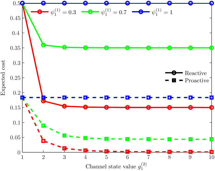
Figure 5: The expected cost for reactive and proactive costs for a single user scenario for time-invariant demand and channel statistics model. The channel probability $\psi_{1}^{(1)}$ and channel state $g_{1}^{(2)}$ are varied with fixed user demand probability to $\bar{\pi}_{1}=0.5$ and fixed $g_{1}^{(1)}=1$.

The impact of channel state on the expected cost for a single user scenario is depicted in Fig. 5. For this scenario, the good channel state $g_{1}^{(2)}$ is increased while the other bad channel state $g_{1}^{(1)}=1$ is kept constant, and the demand probability is set to $\bar{\pi}_{1}=0.5$. When $\psi_{1}^{(1)}=1$ (shown in blue), which means the user always observes $g_{1}^{(1)}$, there is no impact of $g_{1}^{(2)}$ on the expected cost for both the schemes. For $\psi_{1}^{(1)}=0.3$ and $\psi_{1}^{(1)}=0.7$, the cost decreases with increase in $g_{1}^{(2)}$. This is expected, as when one of the channel states becomes good, the applied proactive service is shifted to that channel condition to minimize the cost.

One interesting observation is the decrease in expected cost is significant when when $g_{1}^{(2)}$ is twice $g_{1}^{(1)}$, while beyond this point the reduction in cost is minimal. This phenomenon is related to choice of the fourth-order polynomial for the cost function. It is expected that expected cost will slowly decrease when $g_{1}^{(2)}>2$ for lower-order polynomial cost functions.

V-A3 Impact of proactive service window size on the expected cost

We consider a two-user scenario with demand probability set to $\bar{\pi}_{n}=0.42,n=1,2$, and channel state probabilities set to $\psi_{n}^{(1)}=0.54,n=1,2$, and with same channel state values $g_{n}^{(1)}=0.5,g_{n}^{(2)}=2$, for both users. Under this setting the time averaged cost $\wp_{\mathcal{U}}$ is evaluated when the proactive service window size $T$ is increased. In Fig. 6, we plot the cost of policy $\wp_{\mathcal{U}}$ against asymptotically optimal limit under time-invariant demand and channel statistics. The policy $\wp_{\mathcal{U}}$ converges quickly with $T$ (especially after $T=50$) to the established lower bound $\underline{c}_{\mathcal{U}}(\bar{\boldsymbol{\pi}},\boldsymbol{\Psi})$. To draw more insights, we move on to the more realistic case of time-varying channel statistics in the next subsection.

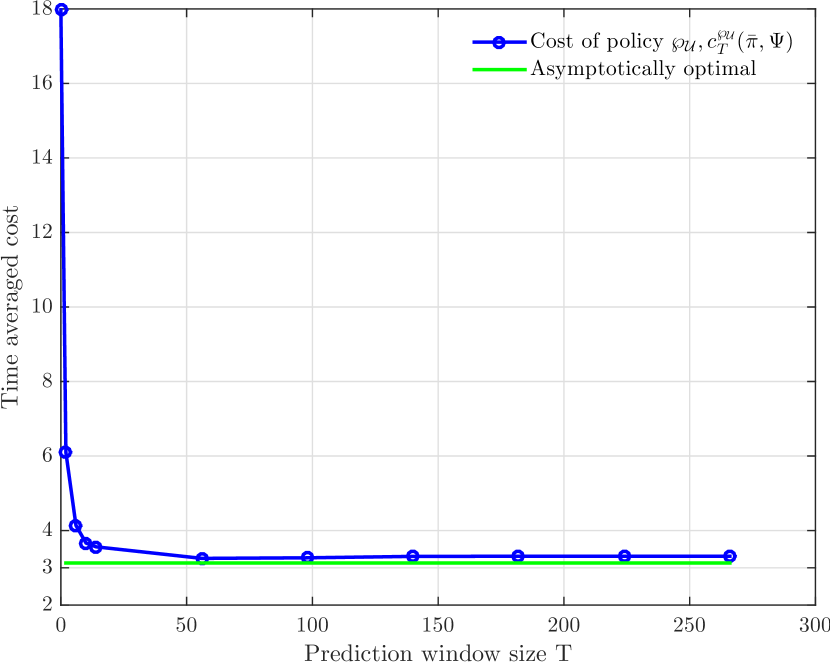
Figure 6: Impact of proactive window size $T$ on achievable cost for time-invariant demand and channel statistics model. The results have been averaged over 40 simulations and for $t=10000$ time slots.

V-B Time-invariant demand and time-varying channel statistics

We consider $N=2$ users and we set demand probability $\bar{\pi}_{n}=0.42,\forall n$ for this scenario in the system. For the time-varying channel statistics, we consider $Q=14$ different channel state probability levels for each state. Similar to earlier numerical results, we consider again two channel states. We set the channel states to $\{g_{n}^{(1)}=0.5,g_{n}^{(2)}=2\}$.

V-B1 Impact of proactive service window size on the expected cost

The time-varying channel probabilities for the channel state $g_{n}^{(1)}$ are (0.8, 0.9, 0.12, 0.24, 0.89, 0.64, 0.9, 0.11, 0.2, 0.27, 0.89, 0.70, 0.59, 0.14). We further assume the channel profile is same for all the users. In Fig. 7, we depict the cost convergence of the policy $\wp_{\mathcal{F}}$ with respect to $\underline{c}_{\mathcal{F}}(\bar{\boldsymbol{\pi}},\boldsymbol{\Psi}^{Q})$ with increase in proactive service window size $T$ under time-invariant demand and time-varying channel statistics. We can clearly observe from the plot that the designed policy $\wp_{\mathcal{F}}$ converges very quickly to the global lower bound $\underline{c}_{\mathcal{F}}(\bar{\boldsymbol{\pi}},\boldsymbol{\Psi}^{Q})$ within proactive service window size of $T=80$. It should be noted that the value of $\underline{c}_{\mathcal{F}}(\bar{\boldsymbol{\pi}},\boldsymbol{\Psi}^{Q})$ is lower compared to $\underline{c}_{\mathcal{U}}(\bar{\boldsymbol{\pi}},\boldsymbol{\Psi})$ (see Fig. 6) for similar settings due to more certain channel statistics.

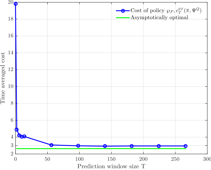
Figure 7: Impact of proactive window size $T$ on achievable cost for time-invariant demand and time-varying channel statistics model. The results have been averaged over 40 simulations and for $t=10000$ time slots.

V-B2 Average load and cost levels of different channel probability levels

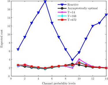
(a)

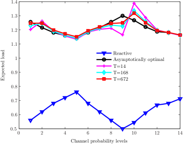
(b)

Figure 8: Inset (a) Average cost levels under reactive and proactive services for time-varying channel statistics. Inset (b) Average load levels under reactive and proactive services for time-varying channel statistics.

In Fig. 8, we show the average cost and load levels for different time periods. For this case, we set the channel probabilities of the channel state $g_{n}^{(1)}$ as (0.4,0.55,0.7,0.8,0.9,0.7,0.55,0.4,0.25,0.36,0.53,0.67,0.7,0.78). We compare proactive scheduler $\wp_{\mathcal{F}}$ for various proactive service window sizes ($T=14,168,672$) against reactive on-time service and asymptotically optimal limit. We can observe in Fig. 8 (a), that the cost of the reactive service varies considerably with changing statistics over time. Reactive service does not possess the flexibility and has to offer service irrespective of the channel conditions. However, it can be observed that the average cost offered by the proactive scheduler is constant. This is due to the fact that the proactive scheduler exhibits flexibility in scheduling and shifts the loads based on the channel conditions. This can be seen in Fig. 8 (b), where the load for the proactive scheduler is less when the channel conditions are worse (i.e., channel time periods $q=1,2,3,4,5$). Furthermore, the load and cost levels of the proactive scheduler approach to corresponding asymptotically optimal limits with increase in $T$. For $T=672$, the proactive scheduler load and cost approach to that of asymptotically optimal (see Fig. 8 (a) and (b)).

VI Conclusions

We studied the impact of demand and channel uncertainties on the design of a proactive scheduler under two scenarios (i) time-invariant demand and channel statistics, (ii) time-invariant demand and time-varying channel statistics. Specifically, we established non-trivial global lower bounds for the two considered scenarios. We showed how to design cyclo-stationary asymptotically optimal proactive service policies that approach such bounds as proactive service window size grow. We observed that the designed proactive resource scheduler provides better performance in terms of lower achievable cost, compared to reactive scheduler. With proactive service, the scheduler has more flexibility to optimize its loads over time depending on the demand and channel levels.

Appendix A Proof of Theorem 1

The optimal value, assuming an optimal policy, is

$$c_{T}^{\mathcal{P}}(\bar{\boldsymbol{\pi}},\boldsymbol{\Psi})=\underset{t\rightarrow\infty}{\limsup}\frac{1}{t}\sum_{l=0}^{t-1}\,\mathbb{E}\biggl{[}C_{d}\bigl{(}\mathbf{L}_{l}^{\mathcal{\mathcal{P}}}(\mathbf{u}_{l},\mathbf{g}_{l})\bigr{)}\biggr{]}$$ (12)

and involves an expectation over all possible sets of requesting users $\mathcal{B}_{l}$ and their channel state realizations $\mathbf{g}_{l}$ at time $l\geq 0$, with associated distribution $P(\mathcal{B}_{l}=\mathcal{B},\mathbf{g}_{l}=\mathbf{g})=P(\mathbf{g}_{l}=\mathbf{g})P(\mathcal{B}_{l}=\mathcal{B})$. Note that both $P(\mathbf{g}_{l}=\mathbf{g})$ and $P(\mathcal{B}_{l}=\mathcal{B})$ are independent of the time $l$. This allows us to write, after substitution of (6) into $L_{n,l}^{\mathcal{\mathcal{P}}}(\mathbf{u}_{n,l},g_{n,l})$:

$$c_{T}^{\mathcal{P}}(\bar{\boldsymbol{\pi}},\boldsymbol{\Psi}) =\underset{t\rightarrow\infty}{\limsup}\frac{1}{t}\sum_{l=0}^{t-1}\sum_{\mathbf{g}\in\mathcal{C}}\sum_{\mathcal{B}\subseteq\mathcal{N}}P_{c}(\mathbf{g})P_{d}(\mathcal{B})$$

$$\times\mathbb{E}\biggl{[}C_{d}\Bigl{(}\Bigl{[}\Bigl{(}S-\sum_{\tau=1}^{T}u_{n,l-\tau}(\tau)$$

$$+\sum_{\tau=1}^{T}u_{n,l}(\tau)\Bigr{)}\Bigr{]}_{n=1}^{N};\mathbf{g}\Bigr{)}\Bigr{|}\mathcal{B},\mathbf{g}\biggr{]}.$$ (13)

Since $C_{d}(\cdot)$ is strictly convex, we can use Jensen’s inequality (i.e., $\mathbb{E}[C_{d}(\cdot)]\geq C_{d}(\mathbb{E}[\cdot])$). The term $\sum_{\tau=1}^{T}u_{n,l-\tau}(\tau)$ is independent on the current channel $\mathbf{g}$ and set $\mathcal{B}$, yielding

$$c_{T}^{\mathcal{P}}(\bar{\boldsymbol{\pi}},\boldsymbol{\Psi}) \geq\underset{t\rightarrow\infty}{\limsup}\frac{1}{t}\sum_{l=0}^{t-1}\sum_{\mathbf{g}\in\mathcal{C}}\sum_{\mathcal{B}\subseteq\mathcal{N}}P_{c}(\mathbf{g})P_{d}(\mathcal{B})$$

$$\times C_{d}\biggl{(}\Bigl{[}\Bigl{(}S-\sum_{\tau=1}^{T}\mathbb{E}[u_{n,l-\tau}(\tau)]\Bigr{)}\delta_{n\in\mathcal{B}}$$

$$+\sum_{\tau=1}^{T}\mathbb{E}[u_{n,l}(\tau)|\mathcal{B},\mathbf{g}]\Bigr{]}_{n=1}^{N};\mathbf{g}\biggr{)}\biggr{]}.$$ (14)

We now push $\underset{t\rightarrow\infty}{\limsup}\frac{1}{t}\sum_{l=0}^{t-1}$ through the summation and through $C_{d}(\cdot)$, using Jensen’s inequality again. Since $\limsup_{t\rightarrow\infty}(-f(t))=-\liminf_{t\rightarrow\infty}(f(t))$, we have

$$c_{T}^{\mathcal{P}}(\bar{\boldsymbol{\pi}},\boldsymbol{\Psi}) \geq\sum_{\mathbf{g}\in\mathcal{C}}\sum_{\mathcal{B}\subseteq\mathcal{N}}P_{c}(\mathbf{g})P_{d}(\mathcal{B})\,C_{d}\biggl{(}\Bigl{[}\delta_{n\in\mathcal{B}}\Bigl{(}S$$

$$-\underset{t\rightarrow\infty}{\liminf}\frac{1}{t}\sum_{l=0}^{t-1}\sum_{\tau=1}^{T}\mathbb{E}[u_{n,l-\tau}(\tau)]\Bigr{)}$$

$$+\underset{t\rightarrow\infty}{\limsup}\frac{1}{t}\sum_{l=0}^{t-1}\sum_{\tau=1}^{T}\mathbb{E}[u_{n,l}(\tau)|\mathcal{B},\mathbf{g}]\Bigr{]}_{n=1}^{N};\mathbf{g}\biggr{)}.$$ (15)

As $C_{d}(x)$ is monotonically increasing in $x$, replacing $\limsup$ on the right hand side of the expression by $\liminf$. We now introduce

$$\tilde{\mu}_{n}\left(\mathcal{B},\mathbf{g}\right)=\underset{t\rightarrow\infty}{\liminf}\frac{1}{t}\sum_{l=0}^{t-1}\sum_{\tau=1}^{T}\mathbb{E}[u_{n,l}^{*}(\tau)|\mathcal{B},\mathbf{g}],$$

and express

$$\mathbb{E}[u_{n,l-\tau}^{*}(\tau)]=\sum_{\mathbf{h}\in\mathcal{C}}\sum_{\mathcal{D}\subseteq\mathcal{N}}P_{c}(\mathbf{h})P_{d}(\mathcal{D})\mathbb{E}[u_{n,l-\tau}^{*}(\tau)|\mathbf{h},\mathcal{D}]$$

allowing us to write

$$c_{T}^{\mathcal{P}}(\bar{\boldsymbol{\pi}},\boldsymbol{\Psi}) \geq\sum_{\mathbf{g}\in\mathcal{C}}\sum_{\mathcal{B}\subseteq\mathcal{N}}P_{c}(\mathbf{g})P_{d}(\mathcal{B})\,C_{d}\biggl{(}\Bigl{[}\delta_{n\in\mathcal{B}}\Bigl{(}S$$

$$-\Bigl{(}\sum_{\mathbf{h}\in\mathcal{C}}P_{c}(\mathbf{h})\sum_{\mathcal{D}\subseteq\mathcal{N}}P_{d}(\mathcal{D})\,\tilde{\mu}_{n}\left(\mathcal{D},\mathcal{\mathbf{h}}\right)\Bigr{)}\Bigr{)}$$

$$+\tilde{\mu}_{n}\left(\mathcal{B},\mathbf{g}\right)\Bigr{]}_{n=1}^{N};\mathbf{g}\biggr{)}.$$ (16)

This proves the theorem.

Appendix B Proof of Theorem 3

It suffices to prove that $\limsup_{T\to\infty}$ $c_{T}^{\wp_{\mathcal{U}}}(\bar{\boldsymbol{\pi}},\boldsymbol{\Psi})$ $=\liminf_{T\to\infty}$ $c_{T}^{\mathcal{P}}(\bar{\boldsymbol{\pi}},\boldsymbol{\Psi})$. We start by $\limsup_{T\to\infty}c_{T}^{\wp_{\mathcal{U}}}(\bar{\boldsymbol{\pi}},\boldsymbol{\Psi})$. Since policy $\wp_{\mathcal{U}}$ is stationary, we can ignore the $\underset{t\rightarrow\infty}{\liminf}\frac{1}{t}\sum_{l=0}^{t-1}$ and write

$$c_{T}^{\wp_{\mathcal{U}}}(\bar{\boldsymbol{\pi}},\boldsymbol{\Psi})= \sum_{\mathcal{B}\subseteq\mathcal{N}}P_{d}(\mathcal{B})\sum_{\mathbf{g}\in\mathcal{C}}P_{c}(\mathbf{g})$$

$$\mathbb{E}\left[C_{d}\left(\Bigl{[}\delta_{n\in\mathcal{B}}(S-\sum_{\tau=1}^{T}u_{n,t-\tau}(\tau))\right.\right.$$

$$+\mu_{n}(\mathcal{B},\mathbf{g})\Bigr{]}_{n=1}^{N};\mathbf{g}\Biggr{)}|\mathcal{B},\mathbf{g}\Biggr{]},$$

since $\sum_{\tau=1}^{T}u_{n,t}(\tau)=\sum_{\tau=1}^{T}T\mu_{n}(\mathcal{B},\mathbf{g})=\mu_{n}(\mathcal{B},\mathbf{g})$.

Note that $\sum_{\tau=1}^{T}u_{n,t-\tau}(\tau)$ is independent of $\mathcal{B}$, $\mathbf{g}$. We introduce a random variable $Z_{T}(\mathcal{D},\mathbf{h})$ which counts the number of occurrences of the pair of requesting set $\mathcal{D}\subseteq\mathcal{N}$ and associated channel gain vector $\mathbf{h}\in\mathcal{C}$, in slots $t-T$, $\cdots$, $t-1$. Then

$$\sum_{\tau=1}^{T}u_{n,t-\tau}(\tau)=\sum_{D\subseteq\mathcal{N}}\sum_{\mathbf{h}\in\mathcal{C}}\frac{\mu_{n}(D,\mathbf{h})Z_{T}(D,\mathbf{h})}{T}$$

By the strong law of large numbers, with probability 1,

$$\limsup_{T\to\infty}\frac{\mu_{n}(D,\mathbf{h})Z_{T}(D,\mathbf{h})}{T}=\mu_{n}(\mathcal{D},\mathbf{h})P_{d}(\mathcal{D})P_{c}(\mathbf{h})$$

By noting that the system load at any time slot is uniformly bounded above, bounded convergence theorem implies

$$\limsup_{T\to\infty}c_{T}^{\wp_{\mathcal{U}}}(\bar{\boldsymbol{\pi}},\boldsymbol{\Psi})=\sum_{B\subseteq\mathcal{N}}P_{d}(\mathcal{B})\sum_{\mathbf{g}\in\mathcal{C}}P_{c}(\mathbf{g})C_{d}\left(\Bigl{[}\delta_{n\in\mathcal{B}}\left(S-\right.\right.\\ \left.\left.\sum_{\mathcal{D}\subseteq\mathcal{N}}\sum_{\mathbf{h}\in\mathcal{C}}\mu_{n}(\mathcal{D},\mathbf{h})P_{d}(\mathcal{D})P_{c}(\mathbf{h})\right)\right.\\ \left.+\mu_{n}(\mathcal{B},\mathbf{g})\Bigr{]}_{n=1}^{N};\mathbf{g}\right)=\underline{c}_{\mathcal{U}}(\bar{\boldsymbol{\pi}},\boldsymbol{\Psi}).$$ (17)

Thus we have established that average expected cost under policy $\wp_{\mathcal{U}}$ attains the global lower bound as proactive service window size grows to infinity. Now by the definition of $c_{T}^{\mathcal{P}}(\bar{\boldsymbol{\pi}},\boldsymbol{\Psi})$ being the minimum possible cost achieved by proactive scheduling with proactive service window $T$, it follows that $\limsup_{T\to\infty}$ $c_{T}^{\wp_{\mathcal{U}}}(\bar{\boldsymbol{\pi}},\boldsymbol{\Psi})$ $=\liminf_{T\to\infty}$ $c_{T}^{\mathcal{P}}(\bar{\boldsymbol{\pi}},\boldsymbol{\Psi})$.

Appendix C Proof of Theorem 4

The optimal value is now

$$c_{T}^{\mathcal{P}}(\bar{\boldsymbol{\pi}},\boldsymbol{\Psi}^{Q})=\underset{t\rightarrow\infty}{\limsup}\frac{1}{t}\sum_{l=0}^{t-1}\,\mathbb{E}\biggl{[}C_{d}\bigl{(}\left[L_{n,l}^{\mathcal{\mathcal{P}}}(\mathbf{u}_{n,l})\right]_{n=1}^{N};\mathbf{g}_{l}\bigr{)}\biggr{]}.$$ (18)

By joint conditioning on all possible sets of requesting users $\mathcal{B}_{l}$, their possible channel state realizations $\mathbf{g}_{l}$, and the slot indices $s$, we can write $c_{T}^{\mathcal{P}}(\bar{\boldsymbol{\pi},}\boldsymbol{\Psi})$ as

$$c_{T}^{\mathcal{P}}(\bar{\boldsymbol{\pi}},\boldsymbol{\Psi}^{Q})$$

$$=\underset{t\rightarrow\infty}{\limsup}\frac{1}{t}\sum_{l=0}^{t-1}\sum_{\mathbf{g}\in\mathcal{C}}\sum_{s\in\mathcal{Q}}\sum_{\mathcal{B}\subseteq\mathcal{N}}\,P(\mathcal{B}_{l}=\mathcal{B},\mathbf{g}_{l}=\mathbf{g},s_{l}=s)$$

$$\times\mathbb{E}\biggl{[}C_{d}\Bigl{(}\left[L_{n,l}^{\mathcal{\mathcal{P}}}(\mathbf{u}_{n,l})\right]_{n=1}^{N};\mathbf{g}_{l}\Bigr{)}\Bigr{|}\mathcal{B}_{l},\mathbf{g}_{l},s_{l}\biggr{]},$$ (19)

Clearly

$$P(\mathcal{B}_{l}=\mathcal{B},\mathbf{g}_{l}=\mathbf{g},s_{l}=s)$$

$$=P_{\mathrm{d}}(\mathcal{B}_{l}=\mathcal{B})P_{c}(\mathbf{g}_{l}=\mathbf{g}|s_{l}=s)P_{\mathrm{s}}(s_{l}=s)$$

$$=P_{\mathrm{d}}(\mathcal{B})P_{c}(\mathbf{g}|s)P_{\mathrm{s}}(s),$$

due to the time-invariant nature of each distribution. Then

$$c_{T}^{\mathcal{P}}(\bar{\boldsymbol{\pi}},\boldsymbol{\Psi}^{Q})$$

$$=\sum_{\mathbf{g}\in\mathcal{C}}\sum_{s\in\mathcal{Q}}\sum_{\mathcal{B}\subseteq\mathcal{N}}P_{\mathrm{d}}(\mathcal{B})P_{c}(\mathbf{g}|s)P_{\mathrm{s}}(s)$$

$$\times\underset{t\rightarrow\infty}{\limsup}\frac{1}{t}\sum_{l=0}^{t-1}\mathbb{E}\biggl{[}C_{d}\Bigl{(}\left[L_{n,l}^{\mathcal{\mathcal{P}}}(\mathbf{u}_{n,l}\right]_{n=1}^{N};\mathbf{g}_{l}\Bigr{)}\Bigr{|}\mathcal{B}_{l},\mathbf{g}_{l},s_{l}\biggr{]},$$ (20)

where the conditioning should be understood as $\mathcal{B}_{l}=\mathcal{B},\mathbf{g}_{l}=\mathbf{g},s_{l}=s$. Now, substituting the definition of $L_{n,l}^{\mathcal{\mathcal{P}}}(\mathbf{u}_{n,l})$ from (6), we have

$$c_{T}^{\mathcal{P}}(\bar{\boldsymbol{\pi}},\boldsymbol{\Psi}^{Q})$$

$$=\sum_{\mathbf{g}\in\mathcal{C}}\sum_{s\in\mathcal{Q}}\sum_{\mathcal{B}\subseteq\mathcal{N}}P_{\mathrm{d}}(\mathcal{B})P_{c}(\mathbf{g}|s)P_{\mathrm{s}}(s)$$

$$\times\underset{t\rightarrow\infty}{\limsup}\frac{1}{t}\sum_{l=0}^{t-1}\mathbb{E}\biggl{[}C_{d}\Bigl{(}\Bigl{[}\delta_{n\in\mathcal{B}}\Bigl{(}S-\sum_{\tau=1}^{T}u_{n,l-\tau}(\tau)\Bigr{)}$$

$$+\sum_{\tau=1}^{T}u_{n,l}(\tau)\Bigr{]}_{n=1}^{N};\mathbf{g}_{l}\Bigr{)}\Bigr{|}\mathcal{B}_{l},\mathbf{g}_{l},s_{l}\biggr{]}.$$ (21)

Applying Jensen’s inequality and accounting for term-wise conditional independencies yields

$$c_{T}^{\mathcal{P}}(\bar{\boldsymbol{\pi}},\boldsymbol{\Psi}^{Q})$$

$$\geq\sum_{\mathbf{g}\in\mathcal{C}}\sum_{s\in\mathcal{Q}}\sum_{\mathcal{B}\subseteq\mathcal{N}}P_{\mathrm{d}}(\mathcal{B})P_{c}(\mathbf{g}|s)P_{\mathrm{s}}(s)$$

$$\times C_{d}\Bigl{(}\Bigl{[}\delta_{n\in\mathcal{B}}(S-\underset{t\rightarrow\infty}{\liminf}\frac{1}{t}\sum_{l=0}^{t-1}\sum_{\tau=1}^{T}\mathbb{E}[u_{n,l-\tau}(\tau)|s_{l}])$$

$$+\underset{t\rightarrow\infty}{\limsup}\frac{1}{t}\sum_{l=0}^{t-1}\sum_{\tau=1}^{T}\mathbb{E}[u_{n,l}(\tau)|\mathcal{B}_{l},\mathbf{g}_{l},s_{l}]\Bigr{]}_{n=1}^{N};\mathbf{g}_{l}\Bigr{)}.$$ (22)

We note that now $u_{n,l-\tau}(\tau)$ depends on the current channel distribution (encoded through $s_{l}$), which is known at time $t-\tau$. Similarly, $u_{n,l}(\tau)$ will depend on the future channel statistics, at times $l+\tau$. Since $s_{l}$ is known, these statistics are also known. Hence, we express

$$\sum_{\tau=1}^{T}\mathbb{E}[u_{n,l}(\tau)\Bigr{|}\mathcal{B},\mathbf{g},s]$$

$$=\sum_{\tau=1}^{T}\mathbb{E}[u_{n,l}(\tau)\Bigr{|}\mathcal{B},\mathbf{g},s_{l}=s,s_{l+\tau}=f_{\tau}(s)]$$

in which $f_{\tau}(s)=\mod(s+\tau,Q)$, due to the cyclo-stationary nature of the channel. We now define

$$\underset{t\rightarrow\infty}{\limsup}\frac{1}{t}\sum_{l=0}^{t-1}\mathbb{E}[u_{n,l}(\tau)]\Bigr{|}\mathcal{B},\mathbf{g},s,s^{\prime}]=\frac{1}{T}\tilde{\mu}_{n}\left(\mathcal{B},\mathbf{g},s,s^{\prime}\right),$$ (23)

where $s,s^{\prime}\in\{0,1,\ldots,Q-1\}$. Similarly, for $\underset{t\rightarrow\infty}{\liminf}\frac{1}{t}\sum_{l=0}^{t-1}\sum_{\tau=1}^{T}\mathbb{E}[u_{n,l-\tau}(\tau)|s_{l}]$, we express as

$$\underset{t\rightarrow\infty}{\liminf}\frac{1}{t}\sum_{l=0}^{t-1}\sum_{\tau=1}^{T}\mathbb{E}[u_{n,l-\tau}(\tau)|s_{l}]$$

$$=\frac{1}{T}\sum_{\mathcal{D}}P_{\mathrm{d}}(\mathcal{D})\sum_{\tau=1}^{T}\sum_{\mathbf{h}}P_{c}(\mathbf{h}|f_{-\tau}(s))\tilde{\mu}_{n}\left(\mathcal{D},\mathbf{h},f_{-\tau}(s),s\right).$$

Finally, this leads to

$$c_{T}^{\mathcal{P}}(\bar{\boldsymbol{\pi}},\boldsymbol{\Psi}^{Q})$$ (24)

$$\geq\sum_{\mathbf{g}\in\mathcal{C}}\sum_{s\in\mathcal{Q}}\sum_{\mathcal{B}\subseteq\mathcal{N}}P_{\mathrm{d}}(\mathcal{B})P_{c}(\mathbf{g}|s)P_{\mathrm{s}}(s)$$

$$\times C_{d}\Bigl{(}\Bigl{[}\delta_{n\in\mathcal{B}}(S-\bar{\mu}_{n}(s))$$

$$+\frac{1}{T}\sum_{\tau=1}^{T}\tilde{\mu}_{n}\left(\mathcal{B},\mathbf{g},s,f_{\tau}(s)\right)\Bigr{]}_{n=1}^{N};\mathbf{g}_{l}\Bigr{)}.$$ (25)

with

$$\bar{\mu}_{n}(s)=\sum_{\mathcal{D}}P_{\mathrm{d}}(\mathcal{D})\frac{1}{T}\sum_{\tau=1}^{T}\sum_{\mathbf{h}}P_{c}(\mathbf{h}|f_{-\tau}(s))\tilde{\mu}_{n}\left(\mathcal{D},\mathbf{h},f_{-\tau}(s),s\right).$$

The expression (24) is the general version of (11), valid for any $T$. For the special case of $T=LQ$,

$$\bar{\mu}_{n}(s) =\sum_{\mathcal{D}}P_{\mathrm{d}}(\mathcal{D})\frac{L}{T}\sum_{s^{\prime}=0}^{Q-1}\sum_{\mathbf{h}}P_{c}(\mathbf{h}|s^{\prime})\tilde{\mu}_{n}\left(\mathcal{D},\mathbf{h},s^{\prime},s\right)$$

$$=\sum_{\mathcal{D}}P_{\mathrm{d}}(\mathcal{D})\sum_{s^{\prime}=0}^{Q-1}P_{\mathrm{s}}(s^{\prime})\sum_{\mathbf{h}}P_{c}(\mathbf{h}|s^{\prime})\tilde{\mu}_{n}\left(\mathcal{D},\mathbf{h},s^{\prime},s\right)$$

and

$$\sum_{\tau=1}^{T}\tilde{\mu}_{n}\left(\mathcal{B},\mathbf{g},s,f_{\tau}(s)\right)=\sum_{s^{\prime}=0}^{Q-1}P_{\mathrm{s}}(s^{\prime})\tilde{\mu}_{n}\left(\mathcal{B},\mathbf{g},s,s^{\prime}\right)$$

in which case (24) becomes (11). It should be noted that the definition (23) implies $0\leq\tilde{\mu}_{n}\left(\mathcal{B},\mathbf{g},s,s^{\prime}\right)\leq S,\,\forall n,\mathcal{B},\mathbf{g},s,s^{\prime}$.

References

- [1] L. S. Muppirisetty, J. Tadrous, A. Eryilmaz, and H. Wymeersch, “On proactive caching with demand and channel uncertainties,” in 53rd Annual Allerton Conference on Communication, Control, and Computing (Allerton), 2015, pp. 1174–1181.
- [2] L. S. Muppirisetty, “Location-aware communications,” Ph.D. dissertation, Chalmers University of Technology, Gothenburg, Sweden, 12 2017.
- [3] C. Song, Z. Qu, N. Blumm, and A.-L. Barabási, “Limits of predictability in human mobility,” Science, vol. 327, no. 5968, pp. 1018–1021, 2010.
- [4] D. Wang, D. Pedreschi, C. Song, F. Giannotti, and A.-L. Barabasi, “Human mobility, social ties, and link prediction,” in 17th ACM SIGKDD International Conference on Knowledge Discovery and Data Mining, 2011, pp. 1100–1108.
- [5] B. S. Jensen, J. E. Larsen, K. Jensen, J. Larsen, and L. K. Hansen, “Estimating human predictability from mobile sensor data,” in IEEE International Workshop on Machine Learning for Signal Processing, 2010, pp. 196–201.
- [6] R. Di Taranto, L. S. Muppirisetty, R. Raulefs, D. Slock, T. Svensson, and H. Wymeersch, “Location-aware communications for 5G networks,” IEEE Signal Processing Magazine, vol. 31, no. 6, pp. 102–112, Nov 2014.
- [7] L. S. Muppirisetty, T. Svensson, and H. Wymeersch, “Spatial wireless channel prediction under location uncertainty,” IEEE Transactions on Wireless Communications, vol. 15, no. 2, pp. 1031–1044, 2016.
- [8] M. Malmirchegini and Y. Mostofi, “On the spatial predictability of communication channels,” IEEE Transactions on Wireless Communications, vol. 11, no. 3, pp. 964–978, 2012.
- [9] S.-J. Kim, E. Dall’Anese, and G. Giannakis, “Cooperative spectrum sensing for cognitive radios using kriged Kalman filtering,” IEEE Journal of Selected Topics in Signal Processing, vol. 5, no. 1, pp. 24–36, 2011.
- [10] G. Piro, L. A. Grieco, G. Boggia, R. Fortuna, and P. Camarda, “Two-level downlink scheduling for real-time multimedia services in lte networks,” IEEE Transactions on Multimedia, vol. 13, no. 5, pp. 1052–1065, 2011.
- [11] N. Bui, M. Cesana, S. A. Hosseini, Q. Liao, I. Malanchini, and J. Widmer, “Anticipatory networking in future generation mobile networks: a survey,” arXiv preprint arXiv:1606.00191, 2016.
- [12] F. Capozzi, G. Piro, L. A. Grieco, G. Boggia, and P. Camarda, “Downlink packet scheduling in lte cellular networks: Key design issues and a survey,” IEEE Communications Surveys & Tutorials, vol. 15, no. 2, pp. 678–700, 2013.
- [13] J. Tadrous and A. Eryilmaz, “On optimal proactive caching for mobile networks with demand uncertainties,” IEEE/ACM Transactions on Networking, vol. 24, pp. 2715–2727, Oct. 2016.
- [14] R. Atawia, H. Abou-zeid, H. S. Hassanein, and A. Noureldin, “Robust resource allocation for predictive video streaming under channel uncertainty,” in IEEE Global Communications Conference, Dec 2014, pp. 4683–4688.
- [15] H. Abou-zeid, H. S. Hassanein, and S. Valentin, “Optimal predictive resource allocation: Exploiting mobility patterns and radio maps,” in IEEE Global Communications Conference, Dec 2013, pp. 4877–4882.
- [16] H. Abou-Zeid and H. S. Hassanein, “Predictive green wireless access: exploiting mobility and application information,” IEEE Wireless Communications, vol. 20, no. 5, pp. 92–99, October 2013.
- [17] S. Mekki and S. Valentin, “Anticipatory quality adaptation for mobile streaming: Fluent video by channel prediction,” in 16th International Symposium on A World of Wireless, Mobile and Multimedia Networks (WoWMoM), June 2015, pp. 1–3.
- [18] J. Lee and N. Jindal, “Asymptotically optimal policies for hard-deadline scheduling over fading channels,” IEEE Transactions on Information Theory, vol. 59, no. 4, pp. 2482–2500, 2013.
- [19] M. Zafer and E. Modiano, “Minimum energy transmission over a wireless channel with deadline and power constraints,” IEEE Transactions on Automatic Control, vol. 54, no. 12, pp. 2841–2852, Dec 2009.
- [20] L. Huang, S. Zhang, M. Chen, and X. Liu, “When backpressure meets predictive scheduling,” in Proceedings of the 15th ACM International Symposium on Mobile Ad Hoc Networking and Computing, 2014, pp. 33–42.
- [21] S. Zhang, L. Huang, M. Chen, and X. Liu, “Effect of proactive serving on user delay reduction in service systems,” in The 2014 ACM International Conference on Measurement and Modeling of Computer Systems, 2014, pp. 573–574.
- [22] J. Tadrous, A. Eryilmaz, and H. El Gamal, “Proactive resource allocation: Harnessing the diversity and multicast gains,” IEEE Transactions on Information Theory, vol. 59, no. 8, pp. 4833–4854, 2013.
- [23] S. Mekki, M. Amara, A. Feki, and S. Valentin, “Channel gain prediction for wireless links with kalman filters and expectation-maximization,” in IEEE Wireless Communications and Networking Conference (WCNC), 2016, pp. 1–7.
- [24] Q. Liao, S. Valentin, and S. Stańczak, “Channel gain prediction in wireless networks based on spatial-temporal correlation,” in 16th IEEE International Workshop on Signal Processing Advances in Wireless Communications (SPAWC), 2015, pp. 400–404.
- [25] Y. Mostofi, M. Malmirchegini, and A. Ghaffarkhah, “Estimation of communication signal strength in robotic networks,” in IEEE International Conference onRobotics and Automation (ICRA), 2010, pp. 1946–1951.