Poissonization of Three Dimensional Nonholonomic Dynamics with the Method of Extension

Abstract

In this study we develop a systematic procedure to construct a Poisson operator that describes the dynamics of a three dimensional nonholonomic system. Instead of reducing by symmetry the antisymmetric operator that links the energy gradient to the velocity on the tangent bundle, the system is embedded in a larger space. Here, the extended antisymmetric operator, which preserves the original equations of motion, satisfies the Jacobi identity in a conformal fashion. Thus, a Poisson operator can be obtained by a further time reparametrization. Such ‘Poissonization’ does not rely on the specific form of the Hamiltonian function. The theory is applied to calculate the equilibrium distribution function of a non-Hamiltonian ensemble.

I Introduction

Nonholonomic dynamical systems Bloch can be characterized in terms of an energy integral (Hamiltonian function) and an antisymmetric operator (or almost Poisson operator) that fails to satisfy the Jacobi identity of Hamiltonian mechanics Mor . These systems arise in the presence of non-integrable constraints Frankel that limit the accessible regions of the phase space Schaft . In addition to the constrained motion of rolling rigid bodies deLeon , and certain systems in molecular dynamics Sergi_1 , the Landau-Lifshitz equation of ferromagnetism Landau_2 , and the $\boldsymbol{E}\times\boldsymbol{B}$ (E cross B) drift equation of plasma dynamics Cary are examples in which the Jacobi identity can be violated Sato6 .

Such violation not only prevents the existence of phase space variables, but has a critical role in determining the dynamical properties of the system Chandre . In a recent paper Sato6 we have further shown that the rupture of the Hamiltonian structure has fundamental implications for the formulation of statistical mechanics, because one cannot rely on the invariant measure provided by Liouville’s theorem in the Hamiltonian setting Sato .

In order to formulate a statistical theory of conservative systems (i.e. systems that admit an energy integral but do not necessarily satisfy the Jacobi identity) it is therefore natural to explore the possibility of ‘repairing’ the antisymmetric operator governing the equations of motion, and thus recover phase space coordinates. In doing so, the method of reduction by symmetry Bates ; Bloch2 ; GarciaN2007 ; Balseiro2 is not particularly helpful because it relies on the specific form of the Hamiltonian function.

Here, we propose an alternative strategy that consists in embedding the system in a larger space by introducing new degrees of freedom. The resulting extended antisymmetric operator is constructed so that the original equations of motion are preserved, while the Jacobi identity is fulfilled by appropriately choosing a conformal factor Chaplygin ; Balseiro . This factor (a strictly positive real valued function) then determines a time reparametrization by which the system obeys Hamilton’s canonical equations in an extended phase space. The procedure developed here applies to any three dimensional nonholonomic system.

The present paper is organized as follows. In section 2 we introduce the notation used throughout the manuscript. In section 3 we discuss a three dimensional conservative system encountered in plasma dynamics, the so called $\boldsymbol{E}\times\boldsymbol{B}$ drift equation of motion. The procedure to Poissonize three dimensional conservative systems is developed in section 4, and then applied in section 5 to Poissonize the $\boldsymbol{E}\times\boldsymbol{B}$ drift dynamics of section 3. Finally, in section 5 we obtain the equilibrium distribution function of an ensemble of charged particles performing $\boldsymbol{E}\times\boldsymbol{B}$ drift by using the canonical phase space recovered by Poissonization.

II Generalities

Let $\left({x^{1},...,x^{n}}\right)$ be a coordinate system on a smooth manifold $\mathcal{M}$ of dimension $n$ with tangent basis $\left({\partial_{1},...,\partial_{n}}\right)$. A conservative vector field $X\in T\mathcal{M}$ is defined as:

$$X=\mathcal{J}\left({dH}\right)=\mathcal{J}^{ij}H_{j}\partial_{i},$$ (1)

Here the subscript indicates derivation. The bivector $\mathcal{J}\in\bigwedge^{2}T\mathcal{M}$ with $\mathcal{J}^{ij}=-\mathcal{J}^{ji}\in C^{\infty}\left({\mathcal{M}}\right)$ is called antisymmetric operator, and the real valued function $H\in C^{\infty}\left({\mathcal{M}}\right)$ the Hamiltonian. Due to antisymmetry, the Hamiltonian $H$ is a constant of motion, $\mathfrak{L}_{X}H=0$. This is the reason why $X$ is conservative. Nonholonomic mechanical systems admit the representation of equation (1) and are characterized by the violation of the Jacobi identity, which demands the vanishing of the quantity

$$h=\mathcal{J}^{im}\mathcal{J}^{jk}_{m}+\mathcal{J}^{jm}\mathcal{J}^{ki}_{m}+\mathcal{J}^{km}\mathcal{J}^{ij}_{m}.$$ (2)

Hence, a nonholonomic system satisfies $h\neq 0$ somewhere on $\mathcal{M}$. When $h=0$, the antisymmetric operator becomes a Poisson operator, and $X$ qualifies as an Hamiltonian vector field.

In the case $n=3$ of $\mathbb{R}^{3}$, one can write:

$$\boldsymbol{v}=\boldsymbol{w}\times\nabla H,$$ (3)

where $\boldsymbol{v}=\left({\dot{x},\dot{y},\dot{z}}\right)$, and $\boldsymbol{w}$ is a vector field such that $w_{x}=\mathcal{J}^{32}$, $w_{y}=\mathcal{J}^{13}$, and $w_{z}=\mathcal{J}^{21}$. Now the Jacobi identity holds when the quantity:

$$h=\boldsymbol{w}\cdot\nabla\times\boldsymbol{w},$$ (4)

vanishes. Notice that $\boldsymbol{w}\cdot\nabla\times\boldsymbol{w}$ is nothing but the helicity density of $\boldsymbol{w}$. In the following we shall refer to $h$ as the helicity density of $\mathcal{J}$.

System (3) is always subject to the constraint $\boldsymbol{w}\cdot\boldsymbol{v}=0$. This constraint is integrable in the sense of the Frobenius’ theorem Frankel provided that $h=0$. Hence, (3) is Hamiltonian if and only if the constraint is integrable. Integrability implies that locally one has $\boldsymbol{w}=\lambda\nabla C$ for some functions $\lambda$ and $C$. Then, $C$ is a constant of motion called Casimir invariant. Furthermore, if $\boldsymbol{w}=\lambda\nabla C\neq\boldsymbol{0}$, the volume form $\lambda^{-1}dx\wedge dy\wedge dz$ is an invariant measure because $\nabla\cdot\left({\lambda^{-1}\boldsymbol{v}}\right)=0$. Conversely, if one can find a function $g\neq 0$ such that $\nabla\cdot\left({g\boldsymbol{v}}\right)=0$ for any choice of $H$, there exists a function $C$ such that $\boldsymbol{w}=g^{-1}\nabla C$, i.e. $\boldsymbol{w}$ is integrable. We conclude that, when $n=3$, the validity of the Jacobi identity, the existence of a Casimir invariant, and the existence of an invariant measure for any choice of $H$, are locally equivalent conditions.

III The Non-Hamiltonian Plasma Particle

Consider a charged particle moving in a static magnetic field $\boldsymbol{B}$ and under the influence of an electric field $\boldsymbol{E}=-\nabla\phi$. The equation of motion is:

$$m\dot{\boldsymbol{v}}=Z\left({\boldsymbol{v}}\times\boldsymbol{B}+\boldsymbol{E}\right).$$ (5)

Here $m$ is the particle mass and $Z$ the electric charge. Suppose that $m$ is sufficiently small so that the left-hand side of equation (5) can be neglected. If we further take the cross product with the magnetic field $\boldsymbol{B}$, (5) becomes:

$$\boldsymbol{v}_{\perp}=\frac{\boldsymbol{E}\times\boldsymbol{B}}{B^{2}},$$ (6)

where $\boldsymbol{v}_{\perp}$ is the velocity in the direction perpendicular to the magnetic field. We will also assume that the particle does not move along the magnetic field, i.e. $\boldsymbol{v}_{\parallel}=\boldsymbol{v}-\boldsymbol{v}_{\perp}=\boldsymbol{0}$, giving $\boldsymbol{v}=\boldsymbol{v}_{\perp}$. The motion resulting from equation (6) goes under the name of $\boldsymbol{E}\times\boldsymbol{B}$ drift and is the physical motivation behind the present study. We refer the reader to Cary for a systematic derivation.

To simplify the notation we set $Z=1$. Recalling that the particle mass is small, the Hamiltonian of the system is $H=\phi$. The antisymmetric operator is then $\boldsymbol{w}=\boldsymbol{B}/B^{2}$, giving (6) in the form $\boldsymbol{v}=\boldsymbol{w}\times\nabla H$. For this system to be Hamiltonian the Jacobi identity has to be satisfied. In light of (4), this occurs only if (locally) $\boldsymbol{w}=\lambda\nabla C$, i.e. when the magnetic field is a solution to the equation $\boldsymbol{B}=B^{2}\lambda\nabla C$ for some appropriate $\lambda$ and $C$. The condition above is verified, for example, in the presence of an harmonic magnetic field $\boldsymbol{B}=\nabla\xi$. In this scenario $\lambda=B^{-2}$ and $C=\xi$. However, the Jacobi identity does not hold in the presence of a non-integrable magnetic field, implying that $\boldsymbol{E}\times\boldsymbol{B}$ drift motion in a magnetic field with finite helicity $\boldsymbol{B}\cdot\nabla\times\boldsymbol{B}\neq 0$ cannot be Hamiltonian.

Below we give two examples that highlight the intrinsic difference between the Hamiltonian and the non-Hamiltonian dynamical settings. First, consider the following system representing the motion of a plasma particle performing $\boldsymbol{E}\times\boldsymbol{B}$ drift:

$$\boldsymbol{w}=\left(\cos z+\sin z\right)\partial_{x}+\left(\cos z-\sin z\right)\partial_{y},$$ (7a)

$$H=\frac{1}{2}\left(x^{2}+y^{2}+z^{2}\right).$$ (7b)

The equations of motion read:

$$\boldsymbol{v}=\left(\cos z-\sin z\right)z\partial_{x}-\left(\cos z+\sin z\right)z\partial_{y}+\left[\left(\cos z+\sin z\right)y-\left(\cos z-\sin z\right)x\right]\partial_{z}.$$ (8)

One can verify that $h=2\neq 0$, hence equation (8) is not Hamiltonian with non-integrable constraint $\boldsymbol{w}\cdot\boldsymbol{v}=0$.

Next, consider the motion of a rigid body with angular momentum $\boldsymbol{x}$ and momenta of inertia $I_{x},I_{y},I_{z}$:

$$\boldsymbol{w}=x\partial_{x}+y\partial_{y}+z\partial_{z},$$ (9a)

$$H=\frac{1}{2}\left(\frac{x^{2}}{I_{x}}+\frac{y^{2}}{I_{y}}+\frac{z^{2}}{I_{z}}\right).$$ (9b)

This time the Jacobi identity is satisfied since $\nabla\times\boldsymbol{w}=\boldsymbol{0}$, and the relevant Casimir invariant is the total angular momentum $C=\boldsymbol{x}^{2}/2$, with $\boldsymbol{w}=\nabla C$. Thus, this second system is Hamiltonian, with integrale constraint $C$=constant. The equations of motion are:

$$\boldsymbol{v}=yz\left(\frac{1}{I_{z}}-\frac{1}{I_{y}}\right)\partial_{x}+xz\left(\frac{1}{I_{x}}-\frac{1}{I_{z}}\right)\partial_{y}+xy\left(\frac{1}{I_{y}}-\frac{1}{I_{x}}\right)\partial_{z}.$$ (10)

Figure 1 shows the trajectory of the plasma particle (8) and that of the rigid body (10). Both of them lie on the integral surface of constant energy. However, while the orbit of the rigid body is closed and results from the intersection of the two integral manifolds defined by $H$ and $C=\boldsymbol{x}^{2}/2$, the plasma particle spirals toward a sink and delineates an open path characterized by the non-zero divergence of the conservative vector field (8).

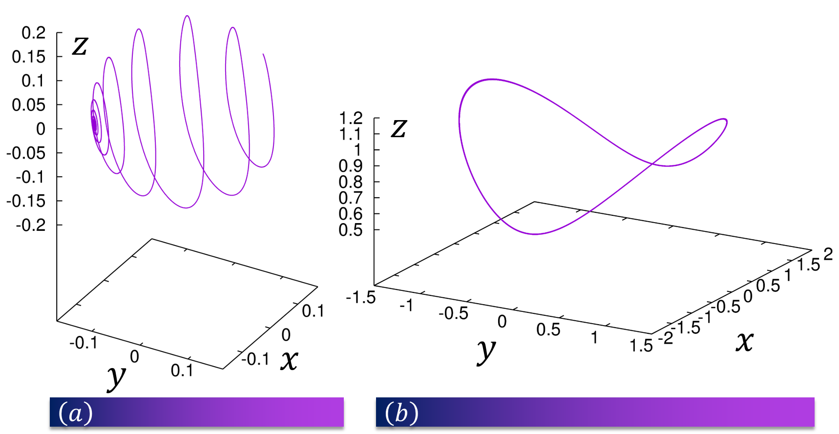
Figure 1: (a): numerical integration of (8). (b): numerical integration of (10).

As discussed at the end of section 2, this example shows that there is an important relationship between the existence of an invariant measure and the Hamiltonian nature of the system. The absence of an invariant measure may be interpreted as the consequence of missing degrees of freedom that would compensate the compressibility of the system. This is why we will need to ‘extend’ the system in order to recover an Hamiltonian structure.

IV Poissonization in Three Dimensions

The purpose of the present section is to develop a systematic procedure to ‘repair’ an arbitrary $3$-dimensional antisymmetric operator and obtain an equivalent Hamiltonian system describing the same dynamics.

IV.1 Extension

The first step of the procedure consists in the embedding of the system in a larger space. The objective is to restore a conformally Poisson structure. To do so in the three dimensional setting, it will be sufficient to add a single new variable $s$. We begin by extending the antisymmetric operator $\mathcal{J}$ in the following manner:

$$\mathfrak{J}=\mathcal{J}+a\,\partial_{x}\wedge\partial_{s}+b\,\partial_{y}\wedge\partial_{s}+c\,\partial_{z}\wedge\partial_{s},$$ (11)

where $\mathfrak{J}$ is the $4\times 4$ extended antisymmetric operator and the coefficients $a,b,c$ have to be determined by requiring that the new operator is conformally Poisson. We remark that these new terms do not affect the original equations of motion since the Hamiltonian function does not depend on the new variable $s$, i.e. $H_{s}=0$.

An antisymmetric operator $\mathfrak{J}$ is a conformally Poisson operator if there exists a strictly positive real valued function $r$ such that $r^{-1}\mathfrak{J}$ satisfies the Jacobi identity. If the matrix $\mathfrak{J}^{ij}$ is invertible with inverse $\Omega_{ij}$ such that $i_{X}\Omega=-dH$ with $\Omega=\sum_{i<j}\Omega_{ij}dx^{i}\wedge dx^{j}\in\bigwedge^{2}T^{\ast}\mathcal{M}$, this condition is equivalent to demanding that:

$$d\left(r\Omega\right)=0,$$ (12)

for some conformal factor $r>0$. Looking for the inverse of (11), we find:

$$\Omega=\frac{1}{aw_{x}+bw_{y}+cw_{z}}\left\{\left[a-s\left(\frac{\partial w_{z}}{\partial y}-\frac{\partial w_{y}}{\partial z}\right)\right]dy\wedge dz+\left[b-s\left(\frac{\partial w_{x}}{\partial z}-\frac{\partial w_{z}}{\partial x}\right)\right]dz\wedge dx+\left[c-s\left(\frac{\partial w_{y}}{\partial x}-\frac{\partial w_{x}}{\partial y}\right)\right]dx\wedge dy+d\left(w_{x}s\right)\wedge dx+d\left(w_{y}s\right)\wedge dy+d\left(w_{z}s\right)\wedge dz\right\}.$$ (13)

With the choice:

$$a=D_{x}+s\left(\frac{\partial w_{z}}{\partial y}-\frac{\partial w_{y}}{\partial z}\right),$$ (14a)

$$b=D_{y}+s\left(\frac{\partial w_{x}}{\partial z}-\frac{\partial w_{z}}{\partial x}\right),$$ (14b)

$$c=D_{z}+s\left(\frac{\partial w_{y}}{\partial x}-\frac{\partial w_{x}}{\partial y}\right),$$ (14c)

the $2$-form $\Omega$ becomes:

$$\Omega=\frac{\mathcal{D}+d\left[s\left({w_{x}dx+w_{y}dy+w_{z}dz}\right)\right]}{\boldsymbol{w}\cdot\left({\boldsymbol{D}+s\nabla\times\boldsymbol{w}}\right)}=\frac{d\left({\mathcal{A}+s\theta}\right)}{\ast\left[\theta\wedge\left({\mathcal{D}+sd\theta}\right)\right]},$$ (15)

Here $\theta=w_{x}dx+w_{y}dy+w_{z}dz$, $\mathcal{D}=d\mathcal{A}=D_{x}dy\wedge dz+D_{y}dz\wedge dx+D_{z}dx\wedge dy$ is an arbitrary closed $2$-form that does not depend on $s$, and $\boldsymbol{D}=\left(D_{x},D_{y},D_{z}\right)$. From equation (15) we see that $\Omega$ is conformally closed with conformal factor:

$$r=\left\lvert{\boldsymbol{w}\cdot\boldsymbol{D}+sh}\right\rvert=\left\lvert{\ast\left({\theta\wedge\mathcal{D}}\right)+sh}\right\rvert,$$ (16)

as long as $r\neq 0$. We will see how to physically determine $\boldsymbol{D}$ in the following section. At this point just notice that by appropriately choosing $\boldsymbol{D}$ one can always set $r>0$.

The extended equations of motion $X=\mathfrak{J}\left(dH\right)$ now read:

$$X=\boldsymbol{w}\times\nabla H-\left(\boldsymbol{D}+s\nabla\times\boldsymbol{w}\right)\cdot\nabla H\,\partial_{s}.$$ (17)

Finally, one can verify that the new equations are divergence free (the extended antisymmetric operator guarantees an invariant measure for any choice of $H$):

$${div}\left(X\right)=\nabla\cdot\left(\boldsymbol{w}\times\nabla H\right)-\nabla\times\boldsymbol{w}\cdot\nabla H=0.$$ (18)

IV.2 Time reparametrization

The second step of the procedure involves a time reparametrization that will give us the desired Poisson structure. This result can be achieved by introducing the new time variable (proper time) $\tau$ satisfying:

$$\frac{d\tau}{dt}=r.$$ (19)

Since by construction $r^{-1}\mathfrak{J}$ satisfies the Jacobi identity, the vector field:

$$Y=r^{-1}X=r^{-1}\mathfrak{J}\left({dH}\right)=r^{-1}\frac{dx^{i}}{dt}\partial_{i}=\frac{dx^{i}}{d\tau}\partial_{i},$$ (20)

is an Hamiltonian vector field expressing the equations of motion with respect to the proper time $\tau$.

V Poissonization of the Non-Hamiltonian Plasma Particle

Here we apply the developed procedure to Poissonize the $\boldsymbol{E}\times\boldsymbol{B}$ drift motion of the plasma particle studied in section $3$.

V.1 The physical meaning of $s$ and $\tau$

First, let us spend some words on the physical meaning of the new variable $s$. From equations (7) and (17), and noting that in this case $\boldsymbol{w}=\boldsymbol{B}/B^{2}$ with $B^{2}=1/2$, we have:

$$\begin{split}\dot{s}&=-\left(\boldsymbol{D}+s\nabla\times\boldsymbol{w}\right)\cdot\nabla H=-\left(\boldsymbol{D}+s\boldsymbol{w}\right)\cdot\nabla H\\ &=-\left(\boldsymbol{B}+s\frac{\boldsymbol{B}}{B^{2}}\right)\cdot\nabla H=-\left(\frac{1}{\sqrt{2}}+s\sqrt{2}\right)\frac{\partial H}{\partial\ell},\end{split}$$ (21)

Here we used the fact that $\boldsymbol{w}=\nabla\times\boldsymbol{w}$ and made the choice $\boldsymbol{D}=\boldsymbol{B}$ (we will justify this choice later). The variable $\ell$ measures the length along a field line ($\partial_{\ell}=\boldsymbol{B}/B$). We define:

$$m\tilde{v}_{\parallel}=\frac{1}{\sqrt{2}}\log{\left[c_{0}\left(\frac{1}{\sqrt{2}}+s\sqrt{2}\right)\right]},$$ (22)

with $c_{0}$ a constant. This implies:

$$m\tilde{v}_{\parallel}=-\frac{\partial H}{\partial\ell}.$$ (23)

Thus, the new variable $\tilde{v}=d\ell/dt$ has the simple interpretation of a velocity in the direction parallel to $\boldsymbol{B}$: the missing degree of freedom $s$ just describes the motion along the magnetic field which was neglected in the original three dimensional description of the dynamics. Inverting equation (22) we also have:

$$s=\frac{1}{2}\left(e^{\sqrt{2}m\tilde{v}_{\parallel}}-1\right).$$ (24)

In the above equation we required that $s=0$ when $\tilde{v}_{\parallel}=0$ so that $c_{0}=\sqrt{2}$ (we will justify this choice later).

What about the meaning of the proper time $\tau$? Using the expression for $r$ equation (16),

$$r=1+sh=1+2s,$$ (25)

Here we used the fact that $\boldsymbol{D}\cdot\boldsymbol{w}=\boldsymbol{B}\cdot\boldsymbol{w}=1$. From (19):

$$\frac{d\tau}{dt}=1+2s=e^{\sqrt{2}m\tilde{v}_{\parallel}}$$ (26)

Thus, the choices $\boldsymbol{D}=\boldsymbol{B}$ and $c_{0}=\sqrt{2}$ are now physically justified because the factor $r$ must be $1$ when $\boldsymbol{w}$ is integrable or $\tilde{v}_{\parallel}=0$, i.e. we must have $d\tau/dt=1$ when the Jacobi identity is satisfied or there is no motion along the magnetic field. If the mass $m$ is small we can expand the exponential to obtain:

$$\frac{d\tau}{dt}=1+\sqrt{2}m\tilde{v}_{\parallel}+o\left(\left(\sqrt{2}m\tilde{v}_{\parallel}\right)^{2}\right).$$ (27)

Neglecting second order terms and noting that $\tilde{v}_{\parallel}\simeq d\ell/dt$, the result is:

$$\tau\simeq t+\sqrt{2}m\ell,$$ (28)

and the proper time $\tau$ can be interpreted as a measure of the distance traveled by the particle along the magnetic field. Note however that the dynamics described by $s$ does not affect the ‘real’ orbit of the particle in $\mathbb{R}^{3}$. Therefore, the distance $\ell$ is ‘fictitious’.

V.2 Poissonization in Cartesian coordinates

We are now ready to write the canonical equations of motion for the plasma particle. Recalling (15), the symplectic $2$-form of interest is:

$$\Omega^{{}^{\prime}}=r\Omega=d\left[\mathcal{A}+s\left(\cos z+\sin z\right)dx+s\left(\cos z-\sin z\right)dy\right]=-d\left\{xd\left[\left(s+\frac{1}{2}\right)\left(\cos z+\sin z\right)\right]+yd\left[\left(s+\frac{1}{2}\right)\left(\cos z-\sin z\right)\right]\right\},$$ (29)

where we used the fact that $\mathcal{A}=\theta/2$. Thus, the canonical variables are:

$$q_{x}=\left(s+\frac{1}{2}\right)\left(\cos z+\sin z\right),$$ (30a)

$$p_{x}=-x,$$ (30b)

$$q_{y}=\left(s+\frac{1}{2}\right)\left(\cos z-\sin z\right),$$ (30c)

$$p_{y}=-y.$$ (30d)

In terms of these new variables we also have:

$$z=\arcsin\left[\frac{q_{x}-q_{y}}{\sqrt{2\left(q^{2}_{x}+q^{2}_{y}\right)}}\right],$$ (31a)

$$s+\frac{1}{2}=\sqrt{\frac{q^{2}_{x}+q^{2}_{y}}{2}},$$ (31b)

$$H=\frac{1}{2}\left(p^{2}_{x}+p^{2}_{y}+\arcsin^{2}\left[\frac{q_{x}-q_{y}}{\sqrt{2\left(q^{2}_{x}+q^{2}_{y}\right)}}\right]\right).$$ (31c)

Here, we chose the positive root for $s+1/2$. Finally, denoting with ^′ derivations with repsect to $\tau$, Hamilton’s canonical equations read:

$$q^{{}^{\prime}}_{x}=H_{p_{x}}=p_{x},$$ (32a)

$$p^{{}^{\prime}}_{x}=-H_{q_{x}}=\frac{-q_{y}}{q^{2}_{x}+q^{2}_{y}}\arcsin\left[\frac{q_{x}-q_{y}}{\sqrt{2\left(q^{2}_{x}+q^{2}_{y}\right)}}\right],$$ (32b)

$$q^{{}^{\prime}}_{y}=H_{p_{y}}=p_{y},$$ (32c)

$$p^{{}^{\prime}}_{y}=-H_{q_{y}}=\frac{q_{x}}{q^{2}_{x}+q^{2}_{y}}\arcsin\left[\frac{q_{x}-q_{y}}{\sqrt{2\left(q^{2}_{x}+q^{2}_{y}\right)}}\right].$$ (32d)

Figure 2 shows a numerical integration of the Hamiltonian system (32). The solution progressively approaches a $2$-dimensional uniform rectilinear motion.

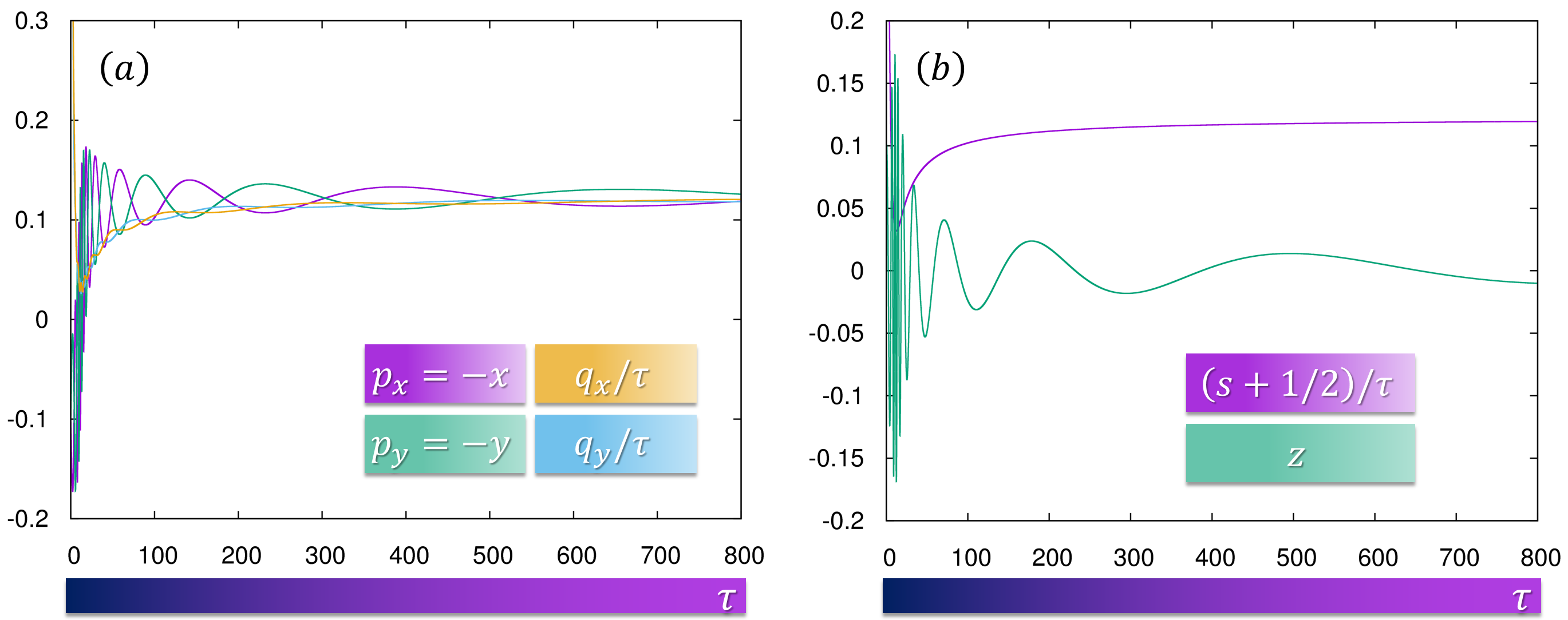
Figure 2: Numerical integration of system (32). (a): evolution with respect to the proper time $\tau$ of $p_{x}$, $q_{x}/\tau$, $p_{y}$, and $q_{y}/\tau$. (b): evolution with respect to the proper time $\tau$ of $\left(s+\frac{1}{2}\right)/\tau$ and $z$.

Finally, observe that in the original time $t$, the equations of motion for the canonical variables $p_{x}$, $q_{x}$, $p_{y}$, and $q_{y}$ take the form:

$$\dot{q}_{x}=r^{-1}H_{p_{x}},$$ (33a)

$$\dot{p}_{x}=-r^{-1}H_{q_{x}},$$ (33b)

$$\dot{q}_{y}=r^{-1}H_{p_{y}},$$ (33c)

$$\dot{p}_{y}=-r^{-1}H_{q_{y}}.$$ (33d)

These equations, which are not canonical, imply that the ‘force’ acting on the particle is only proportional to the gradient of the Hamiltonian with proportionality factor $r^{-1}$. Therefore, the same energy gradient produces different forces depending on the position in space. Such behavior departs from the standard laws of physics and signals the importance of the Jacobi identity in determining the structure of the equations of motion. This inhomogeneity is also the reason why canonical equations can be obtained only by ‘adjusting’ the time variable.

V.3 Poissonization in magnetic coordinates

Consider again the plasma particle of section $3$. By performing an appropriate change of coordinates before the Poissonization procedure, we can simplify the antisymmetric operator $\mathcal{J}$. The simplified form will offer us an insight into the relation between $\mathcal{J}$, which is the result of the abrupt reduction $m\rightarrow 0$ together with $\boldsymbol{v}_{\parallel}\rightarrow\boldsymbol{0}$, and the full dynamics of a magnetized particle. The target coordinates are the so called magnetic coordinates $\left(\ell,\psi,\zeta\right)$ which we will define shortly. This time we shall consider a more general type of magnetic field:

$$\boldsymbol{B}=\nabla\psi\times\nabla\zeta+i\left(\ell,\psi\right)\nabla\psi\times\nabla\ell.$$ (34)

Here $i$ is an arbitrary function of $\ell$ and $\psi$. When $i=0$ equation (34) can conveniently represent a dipole magnetic field. The flux function $\psi$ is chosen so that $\psi=\psi\left(R,z\right)$, where $\left(R,\zeta,z\right)$ is a cylindrical coordinate system $dx\wedge dy\wedge dz\wedge=R\,dR\wedge d\zeta\wedge dz$ with $R$ the radial coordinate in the $\left(x,y\right)$ plane and $\zeta$ the toroidal angle. The coordinate $\ell$ is defined to be the length along the field lines of the poloidal component $\boldsymbol{B}_{p}=\nabla\psi\times\nabla\zeta$ of the magnetic field $\boldsymbol{B}$. In formulae:

$$\partial_{\ell}=\frac{\boldsymbol{B}_{p}}{B_{p}}.$$ (35)

Thus, if $i\neq 0$, the magnetic field has a toroidal component $\boldsymbol{B}_{t}=i\left(\ell,\psi\right)\nabla\psi\times\nabla\ell$. In terms of the new coordinates, the magnetic field $2$-form $\mathfrak{B}$ reads as:

$$\mathfrak{B}=d\psi\wedge d\zeta+id\psi\wedge d\ell.$$ (36)

Note that $d\mathfrak{B}=0$. In order to express $\mathcal{J}$ in the new variables we need some geometrical relationships among tangent and cotangent vectors. We begin by calculating the Jacobian $\mathcal{Q}$ of the coordinate change:

$$\begin{split}\mathcal{Q}&=\nabla\ell\cdot\nabla\psi\times\nabla\zeta=B_{p}.\end{split}$$ (37)

Here we used $\nabla\ell\cdot\partial_{\ell}=1$. Similarly, by using the reciprocity relationships $\nabla u^{j}\cdot\partial_{u^{k}}=\delta_{jk}$ with $\left({u^{1},u^{2},u^{3}}\right)=\left({\ell,\psi,\zeta}\right)$, one obtains the following expressions:

$$\nabla\ell =\frac{1}{\left\lvert\partial_{\psi}\right\rvert^{2}-q^{2}}\left(q\partial_{\psi}+\left\lvert\partial_{\psi}\right\rvert^{2}\partial_{l}\right),$$ (38a)

$$\nabla\psi =\frac{1}{\left\lvert\partial_{\psi}\right\rvert^{2}-q^{2}}\left(\partial_{\psi}+q\partial_{l}\right),$$ (38b)

$$\left\lvert\nabla\ell\right\rvert^{2} =\frac{\left\lvert\partial_{\psi}\right\rvert^{2}}{\left\lvert\partial_{\psi}\right\rvert^{2}-q^{2}},$$ (38c)

$$\left\lvert\partial_{\psi}\right\rvert^{2} =\frac{\left\lvert\nabla\ell\right\rvert^{2}}{R^{2}B_{p}^{2}},$$ (38d)

$$B^{2}_{p} =\frac{1}{R^{2}\left(\left\lvert\partial_{\psi}\right\rvert^{2}-q^{2}\right)}.$$ (38e)

Here $q=-\partial_{\ell}\cdot\partial_{\psi}$. Recalling that the $\boldsymbol{E}\times\boldsymbol{B}$ equation of motion is given by (6) and exploiting (38) with the identities $\nabla u^{j}=\left(\partial_{u^{k}}\times\partial_{u^{m}}\right)/\left(\partial_{u^{j}}\cdot\partial_{u^{k}}\times\partial_{u^{m}}\right)$, $\partial_{u^{j}}=\left(\nabla{u^{k}}\times\nabla{u^{m}}\right)/\left(\nabla{u^{j}}\cdot\nabla{u^{k}}\times\nabla{u^{m}}\right)$ where $j,k,m$ are all different:

$$\dot{\ell} =\nabla\ell\cdot X=\rho\left(iR^{2}H_{\psi}-qH_{\zeta}\right),$$ (39a)

$$\dot{\psi} =\nabla\psi\cdot X=-\rho\left(H_{\zeta}+iR^{2}H_{\ell}\right),$$ (39b)

$$\dot{\zeta} =\nabla\zeta\cdot X=\rho\left(H_{\psi}+qH_{\ell}\right),$$ (39c)

where $\rho=B^{2}_{p}/B^{2}$. Therefore, the bivector $\mathcal{J}$ takes the form:

$$\mathcal{J}=\rho\left(\partial_{\zeta}\wedge\partial_{\psi}+q\partial_{\zeta}\wedge\partial_{\ell}+iR^{2}\partial_{\ell}\wedge\partial_{\psi}\right).$$ (40)

A straightforward application of the Poissonization procedure of section $4$ gives the $4$-dimensional conformal $2$-form:

$$\Omega=\frac{\mathfrak{B}+d\left(s\theta\right)}{\ast\left[\theta\wedge\left(\mathfrak{B}+sd\theta\right)\right]},$$ (41)

where we set $\mathcal{D}=d\mathcal{A}=\mathfrak{B}$ and the kernel of $\mathcal{J}$ is spanned by the covector:

$$\theta=\rho\left(d\ell-qd\psi-iR^{2}d\zeta\right).$$ (42)

Thus, a time reparametrization $d\tau/dt=r$ with conformal factor:

$$r=\ast\left[\theta\wedge\left(\mathfrak{B}+sd\theta\right)\right]=\rho\left\{1+i^{2}R^{2}+s\left[\rho\frac{\partial q}{\partial\zeta}+iR^{2}\left(\frac{\partial\left(q\rho\right)}{\partial\ell}+\frac{\partial\rho}{\partial\psi}\right)-\left(q\partial_{\ell}+\partial_{\psi}\right)\left(iR^{2}\rho\right)\right]\right\},$$ (43)

will give the symplectic $2$-form:

$$\Omega^{{}^{\prime}}=r\Omega=\mathfrak{B}+d\left(s\theta\right)=d\psi\wedge d\zeta+id\psi\wedge d\ell+d\left[s\rho\left(d\ell-qd\psi-iR^{2}d\zeta\right)\right].$$ (44)

Now suppose that $\boldsymbol{B}=\boldsymbol{B}_{p}$, i.e. $i=0$. Then, $\rho=1$ (note that $q_{\zeta}=0$ when $i=0$ due to toroidal symmetry), $\theta\wedge d\theta=(d\ell-qd\psi)\wedge\left(q_{\ell}d\ell\wedge d\psi\right)=0$ and $r=1$. Furthermore, $\Omega$ becomes symplectic:

$$\Omega=d\left(\psi d\zeta+sd\ell-sqd\psi\right).$$ (45)

With the identification $s=v_{\parallel}$ of equation (24) for $m<<1$, the expression (45) is exactly the symplectic $2$-form for the motion of a magnetized particle in a magnetic field of the form $\nabla\psi\times\nabla\zeta$ SatoSelf . From this example we can see that the Poissonization procedure reproduces the correct physics, and that in the presence of a general magnetic field (note that (41) holds for any $\mathfrak{B}$) canonical coordinates can be obtained by operating a time reparametrization.

We conclude this section by giving the antisymmetric operator and the conformal factor for a magnetic field written as:

$$\boldsymbol{B}=\alpha\nabla\psi\times\nabla\zeta+i\nabla\psi\times\nabla\ell+\beta\nabla\zeta\times\nabla\ell.$$ (46)

Here $\alpha$, $\beta$, and $i$ are $3$ arbitrary functions satisfying $\alpha_{\ell}-i_{\zeta}+\beta_{\psi}=0$ to ensure that $d\mathfrak{B}=0$. With the same procedure as above one obtains:

$$\mathcal{J}=\rho\left[\left(\alpha-\beta q\right)\partial_{\zeta}\wedge\partial_{\psi}+\left(\beta\left\lvert\partial_{\psi}\right\rvert^{2}-\alpha q\right)\partial_{\ell}\wedge\partial_{\zeta}+iR^{2}\partial_{\ell}\wedge\partial_{\psi}\right],$$ (47)

The kernel of this operator is spanned by the covector:

$$\theta=\rho\left[\left(\alpha-\beta q\right)d\ell+\left(\beta\left\lvert\partial_{\psi}\right\rvert^{2}-\alpha q\right)d\psi-iR^{2}d\zeta\right]$$ (48)

The conformal factor is:

$$r=\rho\left\{\alpha\left(\alpha-\beta q\right)+\beta\left(\beta\left\lvert\partial_{\psi}\right\rvert^{2}-\alpha q\right)+i^{2}R^{2}+s\left[\left(\alpha-\beta q\right)\left(-\frac{\partial\left(iR^{2}\rho\right)}{\partial\psi}-\frac{\partial\rho\left(\beta\left\lvert\partial_{\psi}\right\rvert^{2}-\alpha q\right)}{\partial\zeta}\right)+\left(\beta\left\lvert\partial_{\psi}\right\rvert^{2}-\alpha q\right)\left(\frac{\partial\rho\left(\alpha-\beta q\right)}{\partial\zeta}+\frac{\partial\left(iR^{2}\rho\right)}{\partial\ell}\right)-iR^{2}\left(\frac{\partial\rho\left(\beta\left\lvert\partial_{\psi}\right\rvert^{2}-\alpha q\right)}{\partial\ell}-\frac{\partial\rho\left(\alpha-\beta q\right)}{\partial\psi}\right)\right]\right\}.$$ (49)

Finally, the symplectic $2$-form recovered after time reparametrization is:

$$\Omega^{{}^{\prime}}=\alpha d\psi\wedge d\zeta+id\psi\wedge d\ell+\beta d\zeta\wedge d\ell+d\left[s\rho\left(\left(\alpha-\beta q\right)d\ell+\left(\beta\left\lvert\partial_{\psi}\right\rvert^{2}-\alpha q\right)d\psi-iR^{2}d\zeta\right)\right].$$ (50)

VI Statistical Mechanics of the Non-Hamiltonian Plasma Particle

In this section we apply the theory to the study of the statistical behavior of an ensemble of particles obeying equation (6).

VI.1 The Jacobian of the coordinate change

By extending system (3) to $4$-dimensions $\boldsymbol{x}=\left(x,y,z,s\right)$, according to equation (18) one obtains the invariant measure (in time $t$):

$$vol^{4}_{\boldsymbol{x}}=dx\wedge dy\wedge dz\wedge ds.$$ (51)

A further time reparametrization, equation (19), gives a symplectic manifold $\boldsymbol{y}=\left(p_{x},q_{x},p_{y},q_{y}\right)$:

$$vol^{4}_{\boldsymbol{y}}=dp_{x}\wedge dq_{x}\wedge dp_{y}\wedge dq_{y}.$$ (52)

The canonical variables $\boldsymbol{y}$ are determined by the specific form of the antisymmetric operator $\boldsymbol{w}$ so that $r\Omega=dp_{x}\wedge dq_{x}+dp_{y}\wedge dq_{y}$. We want to determine the Jacobian of the coordinate change sending (51) to (52). For this purpose, we need the following:

Let $X=d\boldsymbol{x}/dt$ and $Y=d\boldsymbol{y}/d\tau$ be two vector fields with $\boldsymbol{x}=\left(x^{1},...,x^{n}\right)$ and $\boldsymbol{y}=\left(y^{1},...,y^{n}\right)$. Let $g$ be the Jacobian of the coordinate change $vol_{\boldsymbol{y}}^{n}=dy^{1}\wedge...\wedge dy^{n}=g^{-1}dx^{1}\wedge...\wedge dx^{n}=g^{-1}vol_{\boldsymbol{x}}^{n}$. If

$$\mathfrak{L}_{X}vol_{\boldsymbol{x}}^{n}=\mathfrak{L}_{Y}vol_{\boldsymbol{y}}^{n}=0,$$ (53)

then,

$$g=\frac{dt}{d\tau}.$$ (54)

We have:

$$0=\mathfrak{L}_{X}vol_{\boldsymbol{x}}^{n}=di_{X}gvol_{\boldsymbol{y}}^{n}=(-1)^{m-1}d(g\dot{y}^{m})\wedge dy^{1}\wedge...\wedge dy^{m-1}\wedge dy^{m+1}\wedge...\wedge dy^{n}=\frac{1}{g}\frac{\partial}{\partial y^{m}}\left(g\frac{d\tau}{dt}\left(y^{m}\right)^{\prime}\right)vol_{\boldsymbol{x}}^{n}=\frac{d\tau}{dt}\frac{\partial\left(y^{m}\right)^{\prime}}{\partial y^{m}}vol_{\boldsymbol{x}}^{n}+\frac{\left(y^{m}\right)^{\prime}}{g}\frac{\partial}{\partial y^{m}}\left(g\frac{d\tau}{dt}\right)vol_{\boldsymbol{x}}^{n}=\frac{\left(y^{m}\right)^{\prime}}{g}\frac{\partial}{\partial y^{m}}\left(g\frac{d\tau}{dt}\right)vol_{\boldsymbol{x}}^{n}=\frac{1}{g}\frac{d}{d\tau}\left(g\frac{d\tau}{dt}\right)vol_{\boldsymbol{x}}^{n}.$$ (55)

Here, the apex ^′ indicates derivation with respect to $\tau$ and we used the fact that $\mathfrak{L}_{Y}vol_{\boldsymbol{y}}^{n}=0$ if and only if $\partial_{y^{m}}\left(y^{m}\right)^{\prime}=0$. The solution is, up to a scaling constant, $g=dt/d\tau$.

Applying this result to the case $\boldsymbol{x}=\left(x,y,z,s\right)$ and $\boldsymbol{y}=\left(p_{x},q_{x},p_{y},q_{y}\right)$ we conclude that the Jacobian $g$ of the coordinate change is:

$$g=\frac{dt}{d\tau}=r^{-1}=\frac{1}{\boldsymbol{w}\cdot\boldsymbol{D}+sh}.$$ (56)

VI.2 The distribution function of thermodynamic equilibrium

Let $P=P(\boldsymbol{y})$ be the distribution function of an ensemble of particles in the canonical phase space $vol_{\boldsymbol{y}}^{4}$ at thermodynamic equilibrium $\tau\rightarrow\infty$. We want to know how the distribution function $P$ is seen in the initial coordinates $vol_{\boldsymbol{x}}^{4}$. Using the result of equation (56), we have:

$$P\,vol_{\boldsymbol{y}}^{4}=Pr\,vol_{\boldsymbol{x}}^{4},$$ (57)

which implies that the distribution function $f\left(\boldsymbol{x}\right)$ on $vol_{\boldsymbol{x}}^{4}$ is related to $P$ as:

$$f=Pr=P\left({\boldsymbol{w}\cdot\boldsymbol{D}+sh}\right).$$ (58)

From the result above we see that the discrepancy between $P$ and $f$ is controlled by the helicity density $h$. Furthermore, by integrating over the variable $s$, we can calculate the shape of the distribution $\mathcal{F}\left(x,y,z\right)$ in the initial coordinates $(x,y,z)$:

$$\mathcal{F}=\int{fds}=\boldsymbol{w}\cdot\boldsymbol{D}\int{Pds}+h\int{Psds}.$$ (59)

Let us now calculate the form of the distributions at thermodynamic equilibrium. Since $vol_{\boldsymbol{y}}^{4}$ is the preserved volume element of a symplectic manifold spanned by canonical variables, we can exploit the usual formulation of statistical mechanics and define the differential entropy $\Sigma$ of the distribution function $P$:

$$\Sigma=-\int_{V_{\boldsymbol{y}}}{P\log P\,vol_{\boldsymbol{y}}^{4}}.$$ (60)

Here the integral is performed on the whole phase space $V_{\boldsymbol{y}}$. The total number of particles and the total energy $E$ of the ensemble are given by $N=\int_{V_{\boldsymbol{y}}}{P\,vol_{\boldsymbol{y}}^{4}}$ and $E=\int_{V_{\boldsymbol{y}}}{HP\,vol_{\boldsymbol{y}}^{4}}$ respectively. The form of the distribution function at equilibrium is calculated my maximizing the entropy $\Sigma$ under the constraints $N$ and $E$ with the variational principle:

$$\delta\left(\Sigma-\alpha N-\beta E\right)=0.$$ (61)

Here $\alpha$ and $\beta$ are the Lagrange multipliers associated to $N$ and $E$. The result of the variation is:

$$P=\frac{1}{Z}e^{-\beta H}.$$ (62)

In the above equation $Z$ is a normalization constant. Thus, recalling equations (58) and (59), we arrive at the following formulas for $f$ and $\mathcal{F}$:

$$f =\frac{1}{Z}\left(\boldsymbol{w}\cdot\boldsymbol{D}+sh\right)e^{-\beta H},$$ (63a)

$$\mathcal{F} =\frac{\Delta s}{Z}\left(\boldsymbol{w}\cdot\boldsymbol{D}+\frac{\Delta s}{2}h\right)e^{-\beta H}.$$ (63b)

Here $\Delta s=\int{ds}$. The conclusion is that the thermodynamic equilibrium of a three dimensional ensemble governed by an antisymmetric operator departs from the standard Boltzmann distribution of homogeneous probability density on constant energy surfaces. The distortion is controlled by the helicity density $h$, i.e. by the failure of the Jacobi identity.

VI.3 Thermodynamic equilibrium in a non-integrable magnetic field

Consider an ensemble of magnetized particles moving by $\boldsymbol{E}\times\boldsymbol{B}$ drift according to equation (6). The magnetic field $\boldsymbol{B}$ is assumed to be of the form:

$$\boldsymbol{B}=\partial_{x}+\left(\frac{y-\sin y\cos y}{2}-\sin x\right)\partial_{z}.$$ (64)

One can verify that $\mathfrak{B}=d\left[\left(\frac{\sin^{2}y-y^{2}}{4}+y\sin x\right)dx+ydz\right]$. Recalling that the antisymmetric Poisson operator is $\boldsymbol{w}=\boldsymbol{B}/B^{2}$, we have:

$$\boldsymbol{w}=\frac{\partial_{x}+\left(\frac{y-\sin y\cos y}{2}-\sin x\right)\partial_{z}}{1+\left(\frac{y-\sin y\cos y}{2}-\sin x\right)^{2}},$$ (65)

and also,

$$h=\frac{\sin^{2}y}{\left[1+\left(\frac{y-\sin y\cos y}{2}-\sin x\right)^{2}\right]^{2}}.$$ (66)

A typical scenario encountered in magnetized plasmas is quasi-neutrality. In such situation, the electric potential $\phi$ is, on average, zero. Therefore, the Hamiltonian of each ‘massless’ particle is itself zero $H=\phi=0$. However, electrostatic fluctuations $\delta\phi$ generated by random interactions among charged particles drive the ensemble toward equilibrium, which according to (63) is:

$$\mathcal{F}=\frac{\Delta s}{Z}\left\{1+\frac{\Delta s}{2}\frac{\sin^{2}y}{\left[1+\left(\frac{y-\sin y\cos y}{2}-\sin x\right)^{2}\right]^{2}}\right\}.$$ (67)

Here we used equation (66) and set $\boldsymbol{D}=\boldsymbol{B}=\boldsymbol{w}/w^{2}$ as required in the case of $\boldsymbol{E}\times\boldsymbol{B}$ drift. Figure 3 shows a plot of the predicted thermal equilibrium. The shape of the distribution sensibly departs from the flat profile one would expect by a naive application of the entropy principle in the initial (non-Hamiltonian) coordinates. This discrepancy is a consequence of the failure of the Jacobi identity.

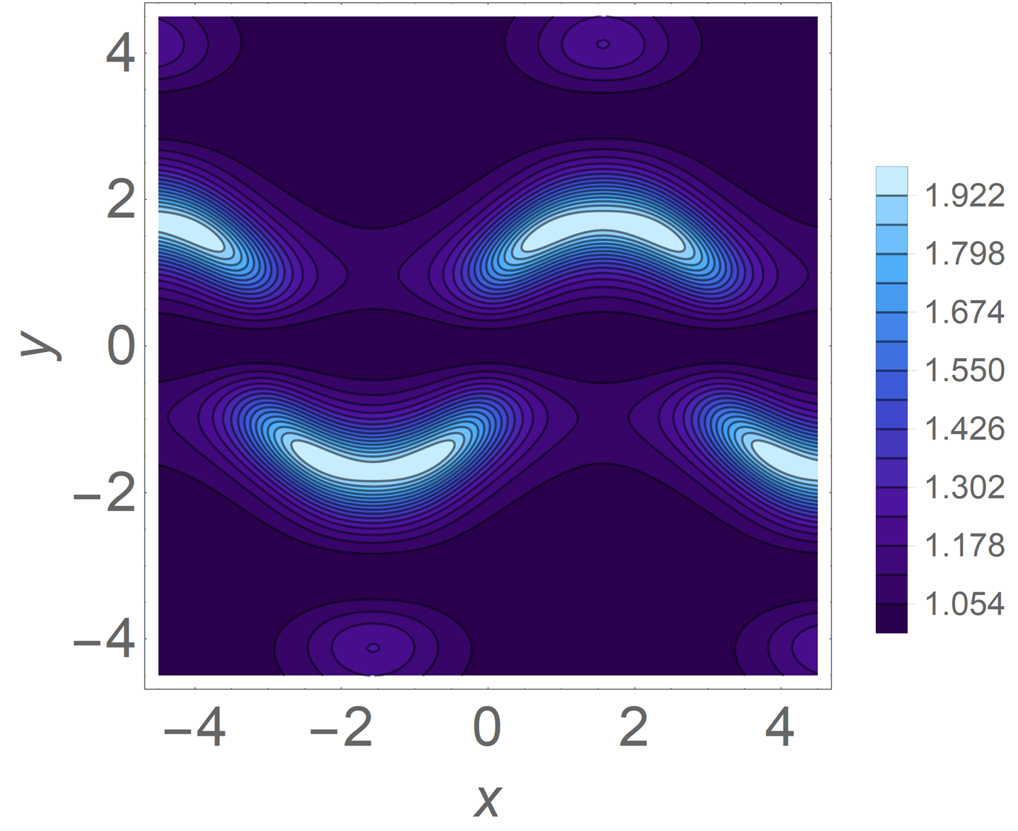
Figure 3: Thermal equilibrium $\mathcal{F}\left(x,y\right)$ by $\boldsymbol{E}\times\boldsymbol{B}$ drift in the magnetic field (64). The inhomogeneous distribution is caused by the failure of the Jacobi identity.

VII Concluding Remarks

Antisymmetric operators arise in the presence of non-integrable constraints. In this study we investigated the problem of repairing an antisymmetric operator in order to recover a Poisson structure.

This issue is encountered when formulating the statistical mechanics of conservative ensembles. Indeed, due to the absence of the invariant measure guaranteed by Liouville’s theorem in the Hamiltonian framework, the usual arguments of statistical mechanics cannot be applied.

In order to overcome these problems, we devised a systematic method to adjust a three dimensional antisymmetric operator by extending it to four dimensions and by operating a proper time reparametrization. The Poissonization procedure does not rely on the existence of special symmetries and therefore does not rely on the specific form of the Hamiltonian function.

A concrete example pertaining to the motion of a charged particle in a magnetic field has been examined. By Poissonizing the system we were able to construct a canonical phase space where the motion is regular and incom- pressible. A physical interpretation of the extended variable and of the proper time was also given: they mimic the motion along the magnetic field.

Finally, we determined the Jacobian of the coordinate change linking the initial coordinates to the extended canonical phase space. We found that the Jacobian is controlled by the helicity density of the antisymmetric operator, which measures the failure of the Jacobi identity. By invoking the principle of maximum entropy in the novel phase space we constructed the distribution function of thermodynamic equilibrium: in the a priori coordinates the shape of the distribution departs from the standard Boltzmann distribution due to the finite helicity density of the antisymmetric operator. The theory has been applied to obtain the equilibrium distribution of an ensemble of charged particles moving by $\boldsymbol{E}\times\boldsymbol{B}$ drift.

VIII Acknowledgments

The author would like to acknowledge useful discussion with Professor Z. Yoshida. The work of N. S. was supported by JSPS KAKENHI Grant No. 16J01486 and No. 18J01729.

References

• (1) Bloch, A. M., Marsden, J. E., Zenkov, D. V., Nonholonomic Dynamics, Notices of the AMS, 52, 320-329 (2005).
• (2) Morrison, P. J. Hamiltonian Description of the Ideal Fluid, Rev. Mod. Phys., 70, 2, 483-491 (1998).
• (3) Frankel, T. The Geometry of Physics, Cambridge University Press, 3rd ed., 165-178 (2012).
• (4) Van Der Shaft, A. J., Maschke, B. M. On the Hamiltonian Formulation of Nonholonomic Mechanical Systems, Reports on Mathematical Physics, 34, 225-233 (1994).
• (5) de LeΓ³n, M. A historical review on nonholonomic mechanics, RACSAM, 106, 191-224 (2012).
• (6) A. Sergi and M. Ferrario, Non-Hamiltonian Equations of Motion With a Conserved Energy, Phys. Rev. E 64, 056125 (2001).
• (7) L. D. Landau and E. M. Lifshitz, On the Theory of the Dispersion of Magnetic Permeability in Ferromagnetic Bodies, Ukr. J. Phys. 53, pp. 14-22 (2008).
• (8) Cary, J. R., Brizard, A. J. Hamiltonian Theory of Guiding-Center Motion, Rev. Mod. Phys., 81, 693-738 (2009).
• (9) N. Sato and Z. Yoshida, Diffusion with finite-helicity field tensor: a new mechanism of generating heterogeneity, arxiv:1712.07817 (2017).
• (10) C. E. Caligan and C. Chandre, Conservative Dissipation: How Important is the Jacobi Identity in the Dynamics?, Chaos 26, 053101 (2016).
• (11) Sato, N., Yoshida, Z. Up-Hill Diffusion, Creation of Density Gradient: Entropy Measure for Systems with Topological Constraints, Phys. Rev. E, 93, 062140 (2016).
• (12) Bates, L., Sniatycki, J., Nonholonomic Reduction, Reports on Mathematical Physics, 32, 99-115 (1993).
• (13) Bloch, A. M., Krishnaprasad, P. S., Marsden, J. E., Murray, R. Nonholonomic Mechanical Systems with Symmetry, Arch. Rational Mech. Anal. 136, 21–99 (1996).
• (14) GarcΓ­a-Naranjo, L. Reduction of Almost Poisson Brackets for Nonholonomic Systems on Lie Groups, Reg. Chaotic Dyn., 12, 4, 365-388 (2007).
• (15) Balseiro, P., The Jacobiator of Nonholonomic Systems and the Geometry of Reduced Nonholonomic Brackets, Arch. Rational Mech. Anal., 214, 453-501 (2014).
• (16) Chaplygin, S. A. On the theory of motion of nonholonomic systems. The reducing multiplier theorem, Regular and Chaotic Dynamics, 13, 369-376 (2008).
• (17) Balseiro, P., Garcia-Naranjo, L. C., Gauge Transformations, Twisted Poisson Brackets and Hamiltonization of Nonholonomic Systems, Arch. Rational Mech. Anal., 205, 267-310 (2012).
• (18) Sato, N., Yoshida, Z., Kawazura, Y. Self-Organization and Heating by Inward Diffusion in Magnetospheric Plasmas, Plasma and Fusion Res., 11, 2401009 (2016).