The galactic rotation curve of a magnetized plasma cloud
Abstract
The rotation curve of a magnetized plasma cloud orbiting in the gravitational potential of a galaxy is calculated by statistical arguments. The working assumption is that a mild magnetic field, decreasing with distance from the galactic center, permeates space. It is shown that the resulting probability density is compatible with a flat rotation curve.
A galaxy rotation curve is the functional relationship between the velocity with which matter rotates around the galactic center, and the radial distance from the galactic center. The discrepancy between the rotation curve predicted by exact balance between gravitational and centripetal accelerations and that obtained from observations Rubin ; Rubin2 is considered indirect evidence for the existence of dark matter Sanders or for the need of modifications of Newtonian gravity Gaugh . Indeed, the galactic mass calculated from observed light distributions Freeman does not match the rotational velocity measured from neutral hydrogen emission in the radio frequency spectrum Gaugh2 . The dark matter density profile needed to justify galactic rotation curves can be modeled with the aid of N-body simulations Navarro ; Read ; Ciotti .
The purpose of this paper is to investigate the effect of a galactic magnetic field on the rotation curve of a plasma cloud (e.g. an H II region) orbiting in the gravitational potential of a galaxy. Galaxies generally exhibit magnetic fields of several that can be seen from radio synchrotron emission both in central regions, spiral arms, and among spiral arms Beck2 ; Chamandy . Magnetic fields play an important role in galactic dynamics and evolution Beck ; Birnboim , and their effect has been studied with MHD simulations Wang . The reason for exploring this problem is that, even in a mildly ionized system (such as the hydrogen clouds Ferriere inside and at the edge of galaxies), any rotational momentum acquired by the ionized component due to magnetization will be gradually transferred to the neutral component by thermalization, thus providing an effective mechanism to stir the whole gas.
In order to determine the rotation curve of the plasma, we will apply the arguments of equilibrium statistical mechanics. This has to be done with care, because the time needed to reach the maximum entropy state for an ideal collisionless system evolving under the effect of long-range interactions Chavanis2 such as gravity LyndenBell ; Chavanis diverges with the number of particles in the ensemble Teles . Instead, quasistationary states depending on the initial conditions of the system can be achieved which exhibit heterogeneous structures Pakter ; Antoniazzi .
In our model, the quasistationary states are obtained as local entropy maxima that entail information on the initial configuration due to the presence of topological constraints that cannot be violated over the timescale of the quasirelaxation (hence the constraints behave as adiabatic invariants Yoshida ). This procedure has a concrete justification once ergodicity is not imposed on the whole phase space, but only over the regions of phase space (the level sets of the constraints) that are dynamically accessible. Such regions are mathematically determined by the Casimir invariants spanning the null-space of the Poisson operator that characterizes the Hamiltonian formulation Morrison of single particle dynamics Sato ; Sato3 .
First, let us determine the rotation curve of a neutral gas within a potential , where is a cylindrical coordinate system. This will be useful when comparing the result for a magnetized plasma system. The assumption on is that , with the radius of a spherical coordinate system.
To formulate a statistical model of the gas, we need to identify the energy (Hamiltonian) of single particle motion (note that, in principle, the particle may represent any mass distribution that is negligible in size with respect to the characteristic scales of the system), any constant of motion , and most importantly the invariant measure (if it exists) associated to the equations of motion. The energy of a particle of mass is:
| (1) |
where , , and . Setting , the equations of motion can be cast in the form , with the antisymmetric matrix:
| (2) |
Since satisfies the Jacobi identity with , where , , and are smooth functions, the equations of motion for are a Hamiltonian system. Then, the invariant measure is provided by the phase space volume element:
| (3) |
Here, the s are the standard canonical momenta. In the presence of a symmetry in the Hamiltonian, by Noether’s theorem, there is an associated constant of motion. For the case of interest, we consider the possibility that the potential is independent of the angle (as is the case of Keplerian rotation). The relevant invariant is therefore the -component of the angular momentum, . If one drops (reduces) the phase , the system becomes -dimensional, and the Poisson matrix becomes degenerate. The null-space will be spanned by the gradient of , implying that any choice of will preserve the vertical component of the angular momentum ( if ), which becomes a Casimir invariant.
The entropy of the gas is given by the functional:
| (4) |
where integration is performed on , and is the probability density on the invariant measure (note that it is crucial that is defined on the measure (3) because the argument of the logarithm must be a probability, see Sato ). The equilibrium probability density can now be evaluated by maximization of entropy under the constraints of total energy , total particle number , and total vertical angular momentum , according to the variational principle (, , and are real constants). The functional form of the integrand in is determined by observing that the conserved quantity must enter the constraint in the same way it enters the Hamiltonian , because, once multiplied by the appropriate chemical potential, must represent the change in energy due to addition or removal of the constant of motion. The result of the variation is:
| (5) |
with a normalization constant such that . The corresponding spatial density is:
| (6) |
Similarly, denoting , the (self) rotation curve is:
| (7) |
If the system is symmetric with respect to all rotations, we may replace with the total angular momentum and obtain analogous formulas:
| (8a) | ||||
| (8b) | ||||
| (8c) | ||||
where is the rotational velocity.
Now consider a body, say a star, orbiting within the gas cloud at radius . The rotation curve of the body can be estimated by assuming that it does not participate to the gas relaxation process. In such case the centripetal acceleration and the gravitational acceleration , with the gravitational constant and the gas cloud mass within , must balance. In the scenario of equation (6) with , we have at large radii on the plane . On the other hand, from the balance equation :
| (9) |
which gives . When the conservation of vertical angular momentum is broken, i.e. , one has , leading to . Similarly, in the scenario of equation (8), implies and , and implies and . Nevertheless, from equations (6), (7), and (8) it is clear that the constraint of total angular momentum is not compatible with a non-decreasing rotation curve for decreasing density. The scenario is different if, in addition to the potential , we assume that a magnetic field permeates the gas cloud, and that particles can interact electromagnetically, as in the case of an ionized gas.
An ionized gas is a plasma. In a magnetic field, a charged particle performs a periodic motion around the local magnetic field line, the cyclotron gyration. The angular frequency of the gyration is given by , with the electric charge and the magnetic field strength. For a proton in a typical galactic environment at the hydrogen ionization temperature within a magnetic field , . The radius of the gyration is given by , where is the velocity of the gyration. The adiabatic invariant associated to cyclotron motion is the magnetic momentum . The motion of a magnetized particle can be expressed in terms of the averaged dynamics of the guiding center (the point in the middle of the cyclotron orbit). The guiding center Hamiltonian is:
| (10) |
with the velocity along the magnetic field. In the following we assume that the magnetic field has the expression , with the so called flux function. In the case of a point dipole magnetic field with a physical constant. It is known Yoshida that the drift velocity around the -axis (such as that of a gravitational orbit in the plane) does not contribute to the guiding center Hamiltonian (10). This is because the canonical angular momentum satisfies due to the smallness of the particle mass, and therefore the kinetic term is negligible. For a particle moving with velocity in a dipole magnetic field with characteristic length scale of one has . Hence, this approximation remains true even for more massive objects bearing a small charge and moving in a galactic environment. Setting , with a length coordinate along the magnetic field, the equations of motion for the guiding center (see Sato2 ) can be cast in the form , where is the antisymmetric matrix:
| (11) |
Here is a geometrical quantity measuring the non-orthogonality of the coordinate system , and its -derivative. The degrees of freedom are only because the phase of the cyclotron gyration does not bear physical significance at the length and time scales of interest. Since satisfies the Jacobi identity, this system is again Hamiltonian. However, the rank of the matrix is , implying that there is a null-space of dimension . It is immediate to verify that the vector spans the null-space of , making a constant of motion since . Integrals like depending only on the form of the Poisson matrix , which entails the geometric properties of space, are Casimir invariants. This is in contrast with conservation of angular momentum, which is a consequence of a symmetry in the Hamiltonian, i.e. a property of matter (remember that conservation of angular momentum can be transformed to a property of space by reducing the associated phase variable). Due to their ‘spatial’ nature, Casimir invariants can distort the metric of the effective phase space of the system. Indeed, the invariant measure of guiding center dynamics is:
| (12) |
Observe how the natural coordinate metric of the system is not , but the measure weighted by magnetic field strength. Hence, while a magnetic field cannot perform work on a particle, it can ‘bend’ space. This has important consequences for statistical mechanics, since the proper entropy measure must now have the form (see Sato ):
| (13) |
where is the probability density on . Maximization of entropy under the constraints of total energy , total particle number , and total magnetic momentum gives the probability density function:
| (14) |
with a normalization constant, and and real constants. The spatial density profile is:
| (15) |
This density profile was first obtained in Yoshida . Furthermore, it has been shown that the probability density (14) is a maximum entropy stationary solution of the Fokker-Planck equation satisfied by an ensemble of magnetized particles (see Sato ; Sato3 ).
In order to calculate the rotation curve, first observe that the guiding center equations of motion demand that:
| (16) |
Here, the subscripts mean derivation. To simplify the expressions, we shall neglect all factors involving the geometric term , which is relatively small and exactly vanishes on the plane in the case of a point dipole magnetic field (if needed, the following calculations can be done by keeping ). The velocity of the rotation around the -axis is thus:
| (17) |
It follows that:
| (18) |
Let us now compare the behaviors of and for different magnetic fields at large radii in the plane . We consider magnetic fields such that , , and with asymptotic behavior for some non-negative real constant . For a point dipole magnetic field and . We further assume that the potential is dominated by the gravitational pull of a mass located in proximity of the center of the system, . This mass could represent the massive central bulge of a galaxy. The potential has thus the form . Notice that, in addition to the self-induced gravitational potential, the electric component of the potential energy is neglected under the assumption that, on average, the plasma charge is canceled by that of a second plasma with opposite charge. It follows that because and the exponential term in (15) approaches at large . Furthermore,
| (19) |
Here we used , , and at . can be evaluated in a similar way:
| (20) |
Then, at , we obtain:
| (21) |
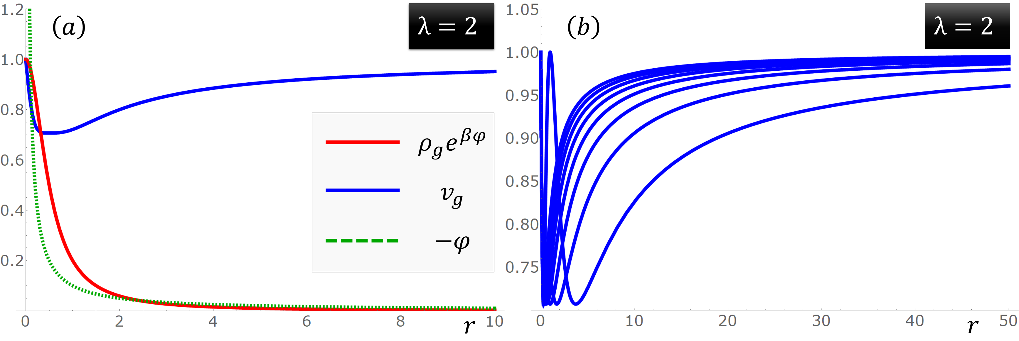
When (point dipole case), . Hence, in the presence of a magnetic field scaling as , the relaxed density profile decreases steeply at large radii, but the rotational velocity exhibits an opposite increasing behavior. This holds true also for with scaling as . Furthermore, observe that for the total mass of the plasma does not diverge with growing , but converges to a constant value. For example, if , the spherical approximation leads to in the limit of large . When the rotational velocity approaches the constant value at large radii. Therefore, a magnetic field scaling as is compatible with a decreasing density profile and a flat rotation curve. For a proton, , with the solar mass, and having units of magnetic flux and representing the order of the magnetic flux through the galaxy surface. If and , . When , the rotation curve falls toward zero at large radii. Figure 1 shows the radial profiles of , , and for the case . We remark that the rotation curve (21) breaks down as soon as the particles cease to be magnetized. Therefore, at distances where the magnetic field becomes negligible we expect the rotation curve to return to that of a neutral gas, equations (7) and (8).
Finally, consider again a body, say a neutral hydrogen atom or a star, orbiting within the plasma cloud at a distance . Under the assumption that the body does not participate to the relaxation process (hence centripetal and gravitational accelerations balance each other), we can calculate its rotation curve from equation (9) by taking into account of both and the plasma mass . In the approximation of spherical symmetry, , one obtains the asymptotic behaviors for , and for .
The research of N. S. was supported by JSPS KAKENHI Grant No. 18J01729.
References
- (1) V. C. Rubin, W. K. Ford, and N. Thonnard, ApJ 225 (1978) pp. L107-L111.
- (2) V. C. Rubin, W. K. Ford, and N. Thonnard, ApJ 238 (1980) pp. 471-487.
- (3) R. H. Sanders, in The Dark Matter Problem: A Historical Perspective (Cambridge University Press, Cambridge, 2010), pp. 38-56.
- (4) S. S. McGaugh, ApJ 609 (2004) pp. 652-666.
- (5) K. C. Freeman, ApJ 160 (1970) pp. 811-830.
- (6) S. S. McGaugh, Galaxies 2 (2014) pp. 601-622.
- (7) J. F. Navarro, ApJ 462 (1996) pp. 563-575.
- (8) J. I. Read, J. Phys. G: Nucl. Part. Phys. 41 063101 (2014).
- (9) L. Ciotti, ApJ 471 (1996) pp. 68-81.
- (10) R. Beck and P. Hoernes, Nature 379 (1996) pp. 47-49.
- (11) L. Chamandy, A. Shukurov, and K. Subramanian, Mon. Not. R. Astron. Soc. 446 (2015) pp. L6-L10.
- (12) R. Beck, Astron. Astrophys. Rev. 4 4 (2016).
- (13) Y. Birnboim, S. Balberg, and R. Teyssier, Mon. Not. R. Astron. Soc. 447 (2015) pp. 3678-3692.
- (14) P. Wang and T. Abel, ApJ 696 1 (2009).
- (15) K. M. Ferrière, Rev. Mod. Phys. 73 (2001) pp. 1031-1061.
- (16) P. H. Chavanis, AIP Conf. Proc. 970 39 (2008).
- (17) P. H. Chavanis, J. Sommeria, and R. Robert, ApJ 471 385 (1996).
- (18) D. Lynden-Bell and R. Wood, Mon. Not. R. Astron. Soc. 138, 495 (1968).
- (19) T. N. Teles, Y. Levin, R. Pakter, and F. B. Rizzato, J. Stat. Mech. P05007 (2010).
- (20) R. Pakter and Y. Levin, Phys. Rev. Lett. 106, 200603 (2011).
- (21) A. Antoniazzi, D. Fanelli, S. Ruffo, and Y. Y. Yamaguchi, Phys. Rev. Lett. 99 040601 (2007).
- (22) Z. Yoshida and S. M. Mahajan, Prog. Theor. Exp. Phys. 2014 073J01 (2014).
- (23) P. J. Morrison, Rev. Mod. Phys. 70 (1998) pp. 467-521.
- (24) N. Sato and Z. Yoshida, Phys. Rev. E 93 062140 (2016).
- (25) N. Sato and Z. Yoshida, Phys. Rev. E 97 022145 (2018).
- (26) N. Sato, Z. Yoshida, and Y. Kawazura, Plasma Fusion Res. 11 2401009 (2016).