Crystalline electric field of Ce in trigonal symmetry: CeIr3Ge7 as a model case
Abstract
The crystalline electric field (CEF) of Ce3+ in trigonal symmetry has recently become of some relevance, for instance, in the search of frustrated magnetic systems. Fortunately, it is one of the CEF case in which a manageable analytic solution can be obtained. Here, we present this solution for the general case, and use this result to determine the CEF scheme of the new compound CeIr3Ge7 with the help of -dependent susceptibility and isothermal magnetization measurements. The resulting CEF parameters K, K and K correspond to an exceptional large CEF splittings of the first and second excited levels, 374 K and 1398 K, and a large mixing between the and the states. This indicates a very strong easy plane anisotropy with an unusual small -axis moment. Using the same general expressions, we show that the properties of the recently reported system CeCd3As3 can also be described by a similar CEF scheme, providing a much simpler explanation for its magnetic properties than the initial proposal. Moreover, a similar strong easy plane anisotropy has also been reported for the two compounds CeAuSn and CePdAl4Ge2, indicating that the CEF scheme elaborated here for CeIr3Ge7 corresponds to an exemplary case for Ce3+ in trigonal symmetry.
pacs:
71.70.Ch,75.10.Dg.I Introduction
Cerium-based intermetallic compounds have been the subject of intensive research during the past decades. This is due to the variety of unconventional and remarkable properties that has been identified in this class of materials, as for instance heavy-fermion superconductivity Steglich et al. (1979); Petrovic et al. (2001), multipolar order Dönni et al. (2000); Sera et al. (2001), Kondo insulator ground state Jaime et al. (2000); Brüning et al. (2010) or non-Fermi-liquid behaviour associated with the presence of a quantum critical point Petrovic et al. (2001); Löhneysen et al. (1994). More recently, systems with geometrical frustrated structures have been considered for the search of spin liquid ground states Dönni et al. (1996); Lucas et al. (2017); Sibille et al. (2015).
The central role is played by the valence instability of the cerium -electron. In the Ce3+ valence state cerium has a local moment with , and total angular momentum , according to Hund’s rules. Ce4+ is non-magnetic. In metals there are then three relevant energy scales which determine the ground state of the system: The crystalline electric field (CEF), the distance of the -electron energy level () from the Fermi level (), , and the hybridization width , with the hybridization strength between the and the conduction electrons and the density of states at the Fermi level (see, e.g., Ref. Bauer (1991) and references therein). Three scenarios should therefore be considered depending on the relative magnitudes of these energy scales: i) For , the system shows intermediate-valence behaviour characterized by a nearly -independent susceptibility at low and Fermi liquid ground state with weakly renormalized quasi particles Lawrence et al. (1981); ii) For , the Kondo effect is present and the system forms a singlet ground state with heavy renormalized quasi particles (heavy fermions) Stewart (1984); iii) For , the system shows a stable valence state and long-range magnetic ordering which is essentially controlled by the RKKY (Ruderman-Kittel-Kasuya-Yosida) interaction. In Ce- and Yb-based systems the ordering temperatures, and thus exchange interactions, are weak ( K) compared to the other rare-earth-based systems, because of the tiny de Gennes factor. The ordering has been found to be usually antiferromagnetic (AFM), but recently several ferromagnetic systems were discovered Brando et al. (2016). Depending on the CEF, Ce-based systems may also exhibit multipolar order: For instance, in the high-symmetry cubic structure the CEF yields to a quartet ground state which allows quadrupolar and AFM order like in Ce3Pd20Ge6 Dönni et al. (2000); Kitagawa et al. (1996) or Ce1-xLaxB6 Fujita et al. (1980); Jang et al. (2017).
In recent past years several Ce-based systems were studied with a trigonal symmetry for the Ce atoms, which is prone to frustration Adroja et al. (1997); Huang et al. (2015); Sibille et al. (2015); Liu et al. (2016); Higuchi et al. (2016); Shin et al. (2018). CeIr3Ge7 is one of these systems and is a prototypical example of case iii) Rai et al. (2018). Since the CEF has a very strong influence on the physical properties, especially in case iii), it is very important to determine the CEF scheme of a compound, i.e., the wave functions and the excitation energies of the different CEF levels. A standard approach is, e.g., to fit the anisotropy of the magnetic susceptibility over a wide range. For the general case, solving the CEF problem and calculating the magnetization implies solving a matrix of size , where is the degeneracy of the ground state multiplet: Thus, for Ce3+, . However, in some cases in which the Ce site has a higher point symmetry, the problem can be highly simplified. A first simplification is to solve the CEF problem not at a finite magnetic field but at , and then to calculate the susceptibility using perturbation theory up to the second order. First and second order correspond to the Curie and the Van Vleck contributions, respectively. Because Ce3+ with an odd number of -electrons is a Kramers system, the size of the relevant matrix is reduced to . For some high symmetry cases, only one of the non-diagonal CEF parameters is allowed. As a consequence, only two of the states mix, while the third one remains a pure one. Accordingly, the matrix reduces to only one non-zero (diagonal) element and a block, which can easily be solved analytically. This is, e.g., the case for Ce3+ in a tetragonal environment, for which simple analytical solutions are available in the literature Fischer and Herr (1987). Ce3+ in a trigonal environment is also such a case for which a manageable analytic solution can be obtained. However, because in the past the number of trigonal Ce-based systems was very limited, this analytical solution has not been published, yet. In the present paper we provide the general solution for the calculation of the CEF scheme and of the susceptibility of Ce in a trigonal environment. We use this general solution to analyze the anisotropic susceptibility of the two recently reported compounds CeIr3Ge7 Rai et al. (2018) and CeCd3As3 Liu et al. (2016). In CeIr3Ge7 we find an unusual large CEF splittings, with the second excited CEF level at about 1400 K. In CeCd3As3 we show that its highly anisotropic susceptibility can be perfectly reproduced by the CEF scheme elaborated here using our general solution. This demonstrates that this compound is an easy plane system with a comparatively small exchange interaction and not an Ising system with a huge anisotropic exchange, as originally proposed in Ref. Liu et al., 2016. We compare the results for CeIr3Ge7 and CeCd3As3 with two further systems with trigonal symmetry, CeAuSn Adroja et al. (1997); Huang et al. (2015) and CePdAl4Ge2 Shin et al. (2018), and show that this point symmetry generally results in a strong easy plane anisotropy and quite similar CEF schemes, making the CEF of CeIr3Ge7 an exemplary case.
II Experimental techniques
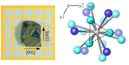
For this work we have used single crystals (see Fig. 1) that were grown using self-flux technique Rai et al. (2018). X-ray diffraction was used for the identification of phase purity of the crystals and Laue method of back scattering reflection was used for the orientation. Using a superconducting quantum interference device (SQUID) and vibrating sample magnetometer (VSM), dc magnetic susceptibility and magnetization were measured between 1.8 and 600 K and in magnetic fields up to 7 T. A comprehensive study of transport, thermodynamic and magnetic properties of CeIr3Ge7 is presented in Ref. Rai et al. (2018).
III Results
CeIr3Ge7 is one compound of a poorly studied RT3M7 (R: rare earth, T: transition metal and M: XIV group element) family which crystallizes in the rhombohedral space group (isostructural to ScRh3Si7 Chabot et al. (1981)) with lattice parameters Å and Å. The Ce atom has a single site at the position with trigonal point symmetry (see Fig. 1). The structure is centrosymmetric.
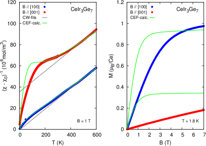
This system is paramagnetic down to the AFM transition temperature of K and presents a large magnetocrystalline anisotropy Rai et al. (2018). This is evidenced by the inverse magnetic susceptibility shown in Fig. 2 (left) between 1.8 and 600 K. The crystallographic -axis is the magnetic hard axis. Above 400 K, follows a Curie-Weiss (CW) behaviour along both field directions. Fitting the data between 400 and 500 K, the CW law yields an effective moment = , very close to that of the free Ce3+ ion of 2.54. We fit only in this temperature range because of the slight upturn of for above 500 K, which is emphasized in Fig. 4 (right). This indicates an additional diamagnetic contribution which is possibly due to the sample holder. This contribution was found to be m3/mol. If subtracted, the high temperature CW fit yields an effective moment of 2.54 as expected for a pure Ce3+ ion (cf. Fig. 5, left).
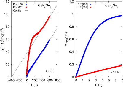
Since the point symmetry of the Ce atom is trigonal, the CEF Hamiltonian has just three parameters. Therefore, to solve exactly the CEF scheme it would be enough to fit the temperature dependence of the susceptibility and the field dependence of the magnetization at low temperature along both principal crystallographic axes. In fact, magnetization at 1.8 K (Fig. 2, right) suggests a saturation moment of about 1 along [100] and much smaller along [001] for the ground state wave function. Before solving the Hamiltonian we can obtain an estimation of the CEF parameter by using the preliminary CW fits shown in Fig. 2 (left): The paramagnetic Weiss temperatures along both principal crystallographic axes [100] and [001] are K and K, respectively. Since the ordering temperatures and thus exchange interactions in Ce-based systems are comparatively weak ( K) because of the tiny de Gennes factor, the anisotropy of at high is dominated by the effect of the crystalline electric field. The Weiss temperatures can be then expressed on the basis of a high-temperature series expansion as a function of the first CEF parameter Bowden et al. (1971), which is therefore a measure of the strength of the magnetocrystalline anisotropy:
| (1) |
Using the paramagnetic Weiss temperatures, we find that = 3.32 meV = 38.5 K. This value is consistent with the large difference between the saturation moments along the [100] and [001] directions observed in magnetization.
We can now use this value as a starting point for evaluating the CEF scheme. For the trigonal point symmetry of the Ce atoms in the crystal, the six-fold degenerate levels split into three Kramers doublets (see Fig. 3). The CEF Hamiltonian is given by
where are CEF parameters and are Steven operators Stevens (1952); Hutchings (1964) which are given by
with operators
For the following calculations we define the crystallographic direction as the quantisation axis and the [100] direction as the axis. Adding the Zeeman term, the global Hamiltonian is
| (2) |
with the Landé -factor for Ce and J/T the Bohr magneton.
The CEF Hamiltonian matrix can be calculated by noting down all the non-zero matrix elements Hutchings (1964). After rearranging the states we obtain
| 0 | |||
| 0 | |||
| 0 | 0 |
where we have defined
The solutions are three doublets of the form
with eigenvalues
where we define
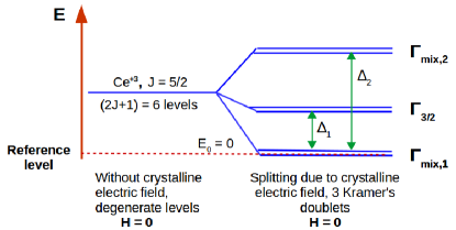
Knowledge of , , allows to simply calculate all other quantities. Our fit to the susceptibility and magnetization data (see below) suggests a CEF level scheme for CeIr3Ge7 as the one shown in Fig. 3 with the as ground state and as first excited state.
The theoretical expression for the magnetic susceptibility with few approximations at different energy levels by Van Vleck is given by
with , , and . Here is the quantization axis, /mol the Avogadro number, J/K the Boltzmann constant and N/A2. The first term is the Curie contribution to the paramagnetic susceptibility and the second term is the Van Vleck susceptibility. For instance, the Curie contribution to the paramagnetic susceptibility for the proposed scheme along both applied field directions can be written as
After substituting the corresponding expectation values (see Appendix), the final paramagnetic and Van Vleck susceptibilities are given by
The total susceptibilities are then given by:
| (3) |
These equations were used to fit the temperature dependence of the susceptibility of CeIr3Ge7 measured at 1 T (see Fig. 5).
Before fitting the data, it is useful to take a closer look at the inverse magnetic susceptibility measured with at low temperatures. This is because along this direction is strongly temperature dependent and a fit to the data can already deliver correct CEF parameters. vs. below 40 K is shown in the left panel of Fig. 4. increases linearly with between 1.8 and 6 K with a slope of mol/m3K indicated by a grey line. This slope yields a CW effective moment of 0.8 and saturation moment of 0.46 which would be in agreement with the saturation magnetization expected from the field dependence of the magnetization measured at 1.8 K (cf. Fig. 1). However, at about 10 K we notice a significant change in slope into another linear increase with mol/m3K which extends to temperatures above 40 K. This would yield a saturation moment of 0.65 which seems to be much too high when compared with the measured magnetization at 1.8 K and with the value of extracted from the Weiss temperatures.
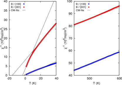
A fit of for at low gives a saturation moment of 1.1 which also agrees with the magnetization measured at 1.8 K. This implies that there is an additional paramagnetic contribution, possibly from a secondary phase, which affects the susceptibility along the hard axis at temperatures above 10 K. Above about 150 K its magnitude becomes negligible. For this reason, we fit our data along the [001] direction with equations 3 in the temperature ranges 1.8 - 6 K and 200 - 600 K. This procedure has been found to be correct, since a fitting of the susceptibility along the [001] direction between 10 and 150 K (with the intention to fit well the hump in in Fig. 2), would give a value of K which can not reproduce either the susceptibility results at high or the low- saturation magnetization. We also considered a possible misalignment of the sample and tried a fit with different weights for both crystallographic directions, but we were never been able to reproduce the data correctly, since this change of slope at 10 K is too pronounced to be reproduced by a misalignment.
The fitted functions together with the experimental data are shown in Fig. 5 for both field directions. In our calculation the quantization -axis is the experimental crystalline [001] direction. We could perfectly fit with in the whole temperature range, the high-temperature part of with as well as its low- part with a single set of CEF parameters. These parameters are listed in Tab. 1. The K is a bit smaller that evaluated from Eq. 1 using the CW temperatures from fits shown in Fig. 5, which is 38.1 K. With the same set of parameters and the Zeeman energy in the Hamiltonian (Eq. 2) we calculated the magnetization at 1.8 K which is shown in the right panel of Fig. 5. The evolution of the magnetization in field does not correspond well to what has been measured, because we have not considered any exchange term in the Hamiltonian: Comparing the initial slope of the experimental data with that of the calculation we can provide an estimation of the exchange interaction which resulted to be 2.4 K, i.e., comparable with the Weiss temperature extracted from the Curie-Weiss fit of the average inverse susceptibility Rai et al. (2018). The saturation moments agree well with those measured by experiments. The small difference is due other paramagnetic contributions as, e.g., from electrons.
CeIr3Ge7
CEF parameters
Energies
Mixing angle
K
K
K
K
K
CeCd3As3
CEF parameters
Energies
Mixing angle
K
K
K
K
K
In fact, the CEF parameters leave as the ground state wave function with a mixing angle and energy splittings between the ground state and the first and second excited states of K 32 meV and K 120 meV. These energy splittings are extremely large when compared with other Ce-based intermetallics which commonly have splittings between 10 and 60 meV Christianson et al. (2004); Pikul et al. (2010); Willers et al. (2012).
With this ground state function, , we can easily calculate the saturation magnetization with field along both crystallographic directions. Considering the Zeeman term , we have
The saturation magnetizations parallel and perpendicular to the -axis are
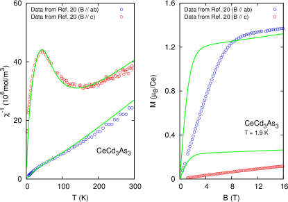
To show the validity and the general character of our calculation we apply the same procedure to the recently discovered system CeCd3As3 Liu et al. (2016). The huge anisotropy of the susceptibility of this compound, as well as the weak dependence of its -axis susceptibility led the authors of Ref. Liu et al., 2016 to propose that CeCd3As3 is a very strong Ising type system with a huge anisotropy of the exchange interaction; the exchange along being orders of magnitude larger than in the basal plane. However, these authors did not try to analyse their data using a CEF model. Susceptibility and magnetization data taken from Ref. Liu et al. (2016) are plotted in Fig. 6. We fit these data with our model and found a very good agreement: The CEF parameters are listed in Tab. 1 and leave as the ground state wave function with a mixing angle and energy splittings between the ground state and the first and second excited states of K 20.8 meV and K 24.3 meV. The saturation magnetizations parallel and perpendicular to the -axis are and . Thus, our analysis shows that the strongly anisotropic susceptibility of CeCd3As3 and its peculiar dependence of the -axis susceptibility can be fully accounted for by the CEF, with a CEF scheme quite similar to that of CeIr3Ge7, except for a smaller overall splitting. Therefore, instead of being a strongly Ising type system, CeCd3As3 is an easy plane XY system with a standard strength of the exchange interaction along both directions. This case demonstrate the importance of doing a CEF analysis before discussing the properties of a rare-earth-based magnetic system, and the value of a general analytical solution to the CEF problem.
In the course of our study we noticed two further systems with Ce3+ in a trigonal (local) environment, CeAuSn Adroja et al. (1997); Huang et al. (2015) and CePdAl4Ge2 Shin et al. (2018). Both show an anisotropy very similar to that of CeIr3Ge7, with a large easy plane susceptibility and a small -axis CEF ground state moment. The CEF of CeAuSn has been well-analyzed in two successive papers Adroja et al. (1997); Huang et al. (2015) leading to a convergent solution quite similar to that of CeIr3Ge7, except for a much smaller overall splitting. In contrast, for CePdAl4Ge2 no CEF analysis was performed, but the similarity of its susceptibility data to those of CeCd3As3 implies a very similar CEF scheme, too. Thus, all the trigonal Ce-based systems investigated recently bear a very similar CEF scheme with a very pronounced easy plane anisotropy and a small -axis CEF ground state moment. This origins from a large positive coefficient, but also from a large mixing coefficient , which is of the same order or even larger than , resulting in a large mixing between the and the states. This is a fundamental difference to purely hexagonal systems with a sixfold point symmetry, where the mixing term is absent, resulting in pure , and CEF doublets.
IV Discussion and Conclusion
A comprehensive analysis of the CEF scheme of Ce3+ in the trigonal point symmetry has been presented. We provided a general analytic solution which can be used to solve the CEF problem and to calculate the anisotropic magnetic susceptibility for Ce in a trigonal surrounding. We have successfully used this solution to analyze the susceptibility of the new compound CeIr3Ge7 and to determine its CEF scheme. This analysis indicates that the ground state doublet in this compound is composed by a large mixing of the and the states, and the first and second excited states are at 374 K and 1398 K, respectively. The latter value is exceptionally large compared to the typical values of K observed in intermetallic Ce-based compounds. Further on, we used the same analytical solution to analyze the anisotropic susceptibility of CeCd3As3. We showed that the anisotropic susceptibility of this compound can be fully accounted for by the CEF, providing a much simpler and standard explanation for its peculiar susceptibility than that originally proposed. We found that two further compounds, CeAuSn and CePdAl4Ge2, presents a very similar anisotropy and accordingly a very similar CEF scheme to that of CeIr3Ge7. This indicates that the CEF of CeIr3Ge7 is an exemplary case for Ce-based systems with trigonal symmetry. This systematic study also shows that in intermetallic Ce-based systems a trigonal environment usually results not only in a large CEF parameter, but also to a large mixing CEF parameter, both leading to a pronounced easy plane behavior.
Our analysis indicates an unusual large overall CEF splitting in CeIr3Ge7. This huge splittings might be connected with the presence of 5 ligands, i.e., nearest-neighbor iridium atoms (see Fig. 1). To check this idea, we have performed band structure calculations using the full-potential local-orbital FPLO code Koepernik and Eschrig (1999). For the exchange and correlation potential, the local density approximation Perdew and Wang (1992) was applied. The calculations were carried out scalar relativistically on a well converged -mesh (202020). The influence of the spin-orbit coupling to the valence states is rather small. We have used the room-temperature data of Ref. Rai et al. (2018) for the lattice parameters and treated the cerium -states as core states (open core approximation).
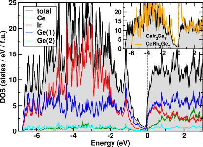
The calculated density of states (DOS) is shown in Fig. 7. The valence band is essentially formed by strongly hybridized Ir (mostly Ir ) and Ge (mostly Ge ) states. A comparison between calculations of CeIr3Ge7 and the fictitious CeRh3Ge7 (we used the same lattice parameters and Wyckoff positions due to the very small difference in atomic size between Ir and Rh) shows that for the Ir-based system the band width, which is a measure of the hybridization, is significantly larger than in the Rh-based compound, indicating that the ligands create a substantially larger crystalline field.
However, the precise estimation of the CEF parameters with density functional theory calculations is very complex and, most importantly, it depends strongly on the hybridization parameter which is not known for CeIr3Ge7. The stronger the larger the crystalline field Huesges et al. (2018). A more quantitative description why this field is so large in CeIr3Ge7 can not be answered here and is beyond the scope of this paper.
V Acknowledgments
We are indebted to M. O. Ajeesh, R. Cardoso, D.-J. Jang and J. Sereni for useful discussions, and D. A. Sokolov for having oriented the crystal. Work at Rice University was supported by the Gordon and Betty Moore Foundation EPiQS Initiative through grant GBMF4417. BKR acknowledges partial support by a QuantEmX grant from ICAM and the Gordon and Betty Moore Foundation through Grant GBMF5305. EM acknowledges travel support from the Alexander von Humboldt Foundation through the Fellowship for Experienced Researchers. *
Appendix A APPENDIX
Appendix B List of matrix elements
We list here all matrix elements for the calculation of the susceptibility.
B.1 Matrix elements for the paramagnetic susceptibility
For the field parallel to -axis:
All other matrix elements are zero:
For field perpendicular to the axis: ; Eigenfunctions of these operators are linear combinations of and , and , and and vice versa.
B.2 Matrix elements for the Van Vleck susceptibility
Here, we assumed the reference level, . Also we notice that
Each of these elements has 4 different combinations of mixed states (a) and (b), evaluated each of them with the operators along both field directions, parallel to the axis and perpendicular to it. For field parallel to the -axis ():
For field perpendicular to the -axis:
References
References
- Steglich et al. (1979) F. Steglich, J. Aarts, C. D. Bredl, W. Lieke, D. Meschede, W. Franz, and H. Schäfer, Phys. Rev. Lett. 43, 1892 (1979).
- Petrovic et al. (2001) C. Petrovic, P. G. Pagliuso, M. F. Hundley, R. Movshovich, J. L. Sarrao, J. D. Thompson, Z. Fisk, and P. Monthoux, J. Phys.: Condens. Matter 13, L337 (2001).
- Dönni et al. (2000) A. Dönni, T. Herrmannsdörfer, P. Fischer, L. Keller, F. Fauth, K. A. McEwen, T. Goto, and T. Komatsubara, J. Phys.: Condens. Matter 12, 9441 (2000).
- Sera et al. (2001) M. Sera, H. Ichikawa, T. Yokoo, J. Akimitsu, M. Nishi, K. Kakurai, and S. Kunii, Phys. Rev. Lett. 86, 1578 (2001).
- Jaime et al. (2000) M. Jaime, R. Movshovich, G. R. Stewart, W. P. Beyermann, M. G. Berisso, M. F. Hundley, P. C. Canfield, and J. L. Sarrao, Nature 405, 160 (2000).
- Brüning et al. (2010) E. M. Brüning, M. Brando, M. Baenitz, A. Bentien, A. M. Strydom, R. E. Walstedt, and F. Steglich, Phys. Rev. B 82, 125115 (2010).
- Löhneysen et al. (1994) H. v. Löhneysen, T. Pietrus, G. Portisch, H. G. Schlager, A. Schröder, M. Sieck, and T. Trappmann, Phys. Rev. Lett. 72, 3262 (1994).
- Dönni et al. (1996) A. Dönni, G. Ehlers, H. Maletta, P. Fischer, H. Kitazawa, and M. Zolliker, J. Phys.: Condens. Matter 8, 11213 (1996).
- Lucas et al. (2017) S. Lucas, K. Grube, C.-L. Huang, A. Sakai, S. Wunderlich, E. L. Green, J. Wosnitza, V. Fritsch, P. Gegenwart, O. Stockert, et al., Phys. Rev. Lett. 118, 107204 (2017).
- Sibille et al. (2015) R. Sibille, E. Lhotel, V. Pomjakushin, C. Baines, T. Fennell, and M. Kenzelmann, Phys. Rev. Lett. 115, 097202 (2015).
- Bauer (1991) E. Bauer, Adv. Phys. 40, 417 (1991).
- Lawrence et al. (1981) J. M. Lawrence, P. S. Riseborough, and R. D. Parks, Rep. Prog. Phys. 44, 1 (1981).
- Stewart (1984) G. R. Stewart, Rev. Mod. Phys. 56, 755 (1984).
- Brando et al. (2016) M. Brando, D. Belitz, F. M. Grosche, and T. R. Kirkpatrick, Rev. Mod. Phys. 88, 025006 (2016).
- Kitagawa et al. (1996) J. Kitagawa, N. Takeda, and M. Ishikawa, Phys. Rev. B 53, 5101 (1996).
- Fujita et al. (1980) T. Fujita, M. Suzuki, T. Komatsubara, S. Kunii, T. Kasuya, and T. Ohtsuka, Solid State Commun. 35, 569 (1980).
- Jang et al. (2017) D. Jang, P. Y. Portnichenko, A. S. Cameron, G. Friemel, A. V. Dukhnenko, N. Y. Shitsevalova, V. B. Filipov, A. Schneidewind, A. Ivanov, D. S. Inosov, et al., npj Quantum Materials 2, 62 (2017).
- Adroja et al. (1997) D. T. Adroja, B. D. Rainford, and A. J. Neville, J. Phys.: Condens. Matter 9, L391 (1997).
- Huang et al. (2015) C. L. Huang, V. Fritsch, B. Pilawa, C. C. Yang, M. Merz, and H. v. Löhneysen, Phys. Rev. B 91, 144413 (2015).
- Liu et al. (2016) Y. Q. Liu, S. J. Zhang, J. L. Lv, S. K. Su, T. Dong, G. Chen, and N. L. Wang, arXiv:1612.03720 (2016).
- Higuchi et al. (2016) S. Higuchi, Y. Noshima, N. Shirakawa, M. Tsubota, and J. Kitagawa, Materials Research Express 3, 056101 (2016).
- Shin et al. (2018) S. Shin, P. F. Rosa, F. Ronning, J. D. Thompson, B. L. Scott, S. Lee, H. Jang, S.-G. Jung, E. Yun, H. Lee, et al., J. Alloys Compd. 738, 550 (2018).
- Rai et al. (2018) B. Rai, J. Banda, M. Stavinoha, R. Borth, M. Nicklas, D. Jang, K. Benavides, D. Sokolov, J. Y. Chan, M. Brando, et al., arXiv:1804.05131 (2018).
- Fischer and Herr (1987) G. Fischer and A. Herr, phys. status solidi (b) 159, K23 (1987).
- Chabot et al. (1981) B. Chabot, N. Engel, and E. Parthé, Acta Crystallogr. Sec. B 37, 671 (1981).
- Bowden et al. (1971) G. J. Bowden, D. S. P. Bunbury, and M. A. H. McCausland, J. Phys. C: Solid State Phys. 4, 1840 (1971).
- Stevens (1952) K. W. H. Stevens, Proc. Phys. Soc. London, Sec. A 65, 209 (1952).
- Hutchings (1964) A. T. Hutchings, Solid State Phys. 16, 227 (1964).
- Christianson et al. (2004) A. D. Christianson, E. D. Bauer, J. M. Lawrence, P. S. Riseborough, N. O. Moreno, P. G. Pagliuso, J. L. Sarrao, J. D. Thompson, E. A. Goremychkin, F. R. Trouw, et al., Phys. Rev. B 70, 134505 (2004).
- Pikul et al. (2010) A. P. Pikul, D. Kaczorowski, Z. Gajek, J. Stȩpie ń Damm, A. Ślebarski, M. Werwiński, and A. Szajek, Phys. Rev. B 81, 174408 (2010).
- Willers et al. (2012) T. Willers, D. T. Adroja, B. D. Rainford, Z. Hu, N. Hollmann, P. O. Körner, Y.-Y. Chin, D. Schmitz, H. H. Hsieh, H.-J. Lin, et al., Phys. Rev. B 85, 035117 (2012).
- Koepernik and Eschrig (1999) K. Koepernik and H. Eschrig, Phys. Rev. B 59, 1743 (1999).
- Perdew and Wang (1992) J. P. Perdew and Y. Wang, Phys. Rev. B 45, 13244 (1992).
- Huesges et al. (2018) Z. Huesges, K. Kliemt, C. Krellner, R. Sarkar, H.-H. Klauß, C. Geibel, M. Rotter, P. Novák, J. Kunes̆, and O. Stockert, New J. Phys. 20, 073021 (2018).